Applying Petroleum the Pressure Buildup Well Test Procedure on Thermal Response Test—A Novel Method for Analyzing Temperature Recovery Period

Abstract

The theory of Thermal Response Testing (TRT) is a well-known part of the sizing process of the geothermal exchange system. Multiple parameters influence the accuracy of effective ground thermal conductivity measurement; like testing time, variable power, climate interferences, groundwater effect, etc. To improve the accuracy of the TRT, we introduced a procedure to additionally analyze falloff temperature decline after the power test. The method is based on a premise of analogy between TRT and petroleum well testing, since the origin of both procedures lies in the diffusivity equation with solutions for heat conduction or pressure analysis during radial flow. Applying pressure build-up test interpretation techniques to borehole heat exchanger testing, greater accuracy could be achieved since ground conductivity could be obtained from this period. Analysis was conducted on a coaxial exchanger with five different power steps, and with both direct and reverse flow regimes. Each test was set with 96 h of classical TRT, followed by 96 h of temperature decline, making for almost 2000 h of cumulative borehole testing. Results showed that the ground conductivity value could vary by as much as 25%, depending on test time, seasonal period and power fluctuations, while the thermal conductivity obtained from the falloff period provided more stable values, with only a 10% value variation.

1. Introduction

The number of installed systems utilizing shallow geothermal energy has constantly increased over the last decade. Although it is common practice to model borehole heat exchangers grid of power less than 30 kW [1] with various software that estimate thermogeological property of the soil, Thermal Response Test (TRT) is the only justifiable method for obtaining the correct properties for certain locations.

The catalogue properties of soil, which are the source of data for the software modeling phase, often lead to undersized systems and functional problems. Soil sample analysis in the laboratory is too expensive for everyday use. Considering this, TRT is also the most profitable method for modeling long-term operating systems. Inaccuracies in the estimation of thermal properties from TRT are mostly caused by outdoor effects. It is necessary to recognize and reduce the atmospheric influences, as well as changes in ambient temperature. Energy dissipation from the pipes above the ground results in a higher value of estimated thermal conductivity, and may lead to the undersizing of the future system installation.

Steep changes caused by the demand of consumers in the local electrical grid will cause fluctuation of the power provided for electric heaters in TRT equipment, leading to variation in the rate of heat transfer to the borehole fluid. This directly affects the entering source temperature (EST), as well as the orderliness of the results of the measurement, and the change of temperature over time, which is a source for calculating the thermal conductivity of the found and borehole thermal resistance. Therefore, TRT should be performed using 24 h cycles, because it is easier to link discrepancies in the measurement with the daily oscillation patterns of electricity use. Prerequisites for credible calculations based on TRT measurements are described in numerous pieces of research and handbooks.

The novel method for TRT presented in this paper could achieve more precise determination of the thermal properties of the ground. It is based on theoretical and experiential methods from petroleum engineering, which has been utilized in practice for almost century, and where it is possible to identify similarities resulting from its use of the same theoretical framework for describing pressure behavior and heat conduction based on the solution of the diffusivity equation. Therefore, our recommendation is to always conduct analysis of thermal recovery period after performing classical TRT. Such prolonged TRT procedures could decrease chance of errors in interpretation due to the fluctuation of voltage in the public electrical grid and the effect of test duration on the final calculations of ground thermal properties. Furthermore, the presented method is suitable for diminishing the effects of ambient temperature interference, which can affect the values of ground thermal conductivity. This is especially true during the winter season, when there is a large difference between the air temperature and fluid inside the pipes during TRT. However, during the TRT recovery period there is a significantly lower temperature difference, due to the smaller heat flux between the surface equipment and surrounding.

2. Literature Overview

The Duration of Thermal Response Test is one of the most discussed parameters in interpretation procedures. The ASHRAE Handbook [1] recommends that TRT be performed for at least 36 to 48 h. Bujok et al. [2] presented measurements conducted on experimental underground heat storage. TRT was performed on eight boreholes with various test-time durations on identical ground environments. Software simulation of thermal conductivity showed that data recorded for the first 24 h of TRT deviated by up to 7.8% compared to the results of TRT provided for 70 h. Furthermore, borehole thermal resistance value obtained from 24-h long TRT differs by up to 17.9% from values calculated based on 70-h long TRT.

The least discussed influence on the credibility of TRT is the variation of ambient temperature, which can strongly affect the measured temperature results of circulating fluid. Bandos et al. [3] first introduced a method whereby the effect of atmospheric conditions is subtracted by using air temperature data for the time at which the test was conducted. Application of this method reduces the oscillation of the thermal conductivity value from 30% to 10% of the mean value. It has been shown in research that the delay of the ambient to mean fluid temperature is about 3 h.

Borinaga-Trevino et al. [4] developed a method to reduce the influence of atmospheric conditions on the TRT. The main advantage is that it is not necessary to know its physical origin; rather, it is based on analyzing the influence of the chosen time interval in order to fit the data of the infinite line source theory (ILS) when predicting the ground thermal conductivity. Two TRTs were analyzed, each with different equipment and levels of isolation from the environment. They concluded that poorly isolated TRT equipment that is exposed to variable ambient conditions can lead to an error of ±33% in determining the thermal conductivity of the ground, depending on the climate and season.

Signorelli et al. [5] tested the duration of the TRT for the evaluation of ground thermal properties, comparing the results from 3D finite element numerical models with the results from synthetic line source solutions. Research has focused on the estimation of the time t0, which denotes the point in time after the start of the test after which the data will not be affected by the lower thermal conductivity of the tubes and grouting material and the effect of unsteady heat transfer. In this case, the simulated 200 h test in the numerical model was evaluated for t0 values of 10 h, 20 h, 40 h, and 60 h, and variable values for the end of the test, tE, to the extent t0 < tE < 200 h. According to the results, accurate definition of t0 has a more significant impact on values of calculated thermal conductivity than the total duration of test.

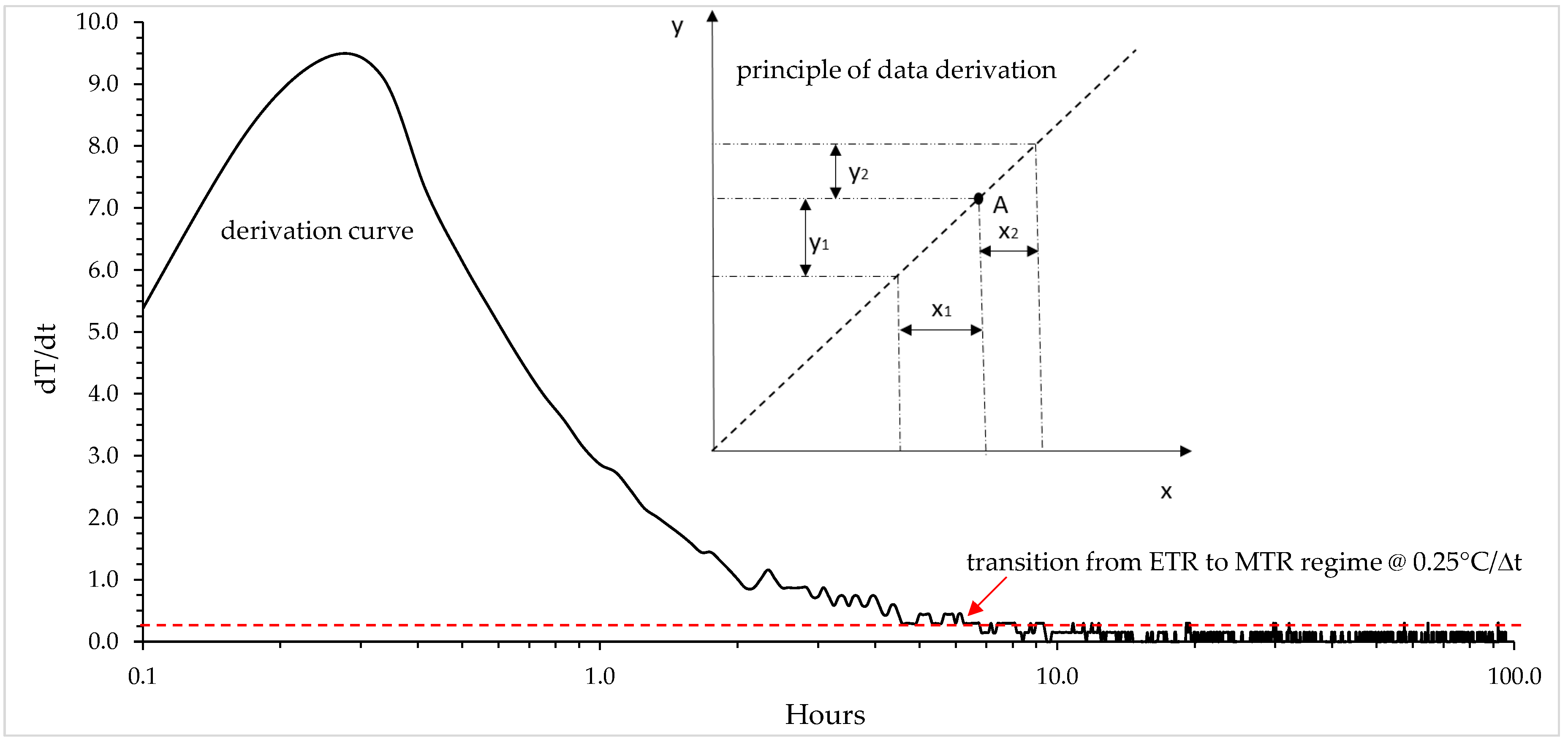
A novel method for the determination of the duration of the unsteady state was presented by Kurevija et al. [6], in which a derivation curve—a method from well testing in petroleum engineering—was applied to recorded temperature data. It is based on monitoring the change of temperature for certain small periods of time versus cumulative time (dT/dt vs. time). The dampening temperature change curve precisely shows the time after which the change of temperature drops below 0.25 °C per 5 min interval, as an arbitrarily established value. Such determination of the beginning time of semi-steady-state heat transfer is much more accurate than the standard method from Gehlin [7], where the value of thermal diffusivity needs to be assumed.

Badenes et al. [8] investigated the influence of operational parameters during TRT, distinguishing the importance of heat rejection control. Research shows that, when a proportional-integral-derivative (PID) controller is used, the impact of environmental temperature fluctuations is decreased, fluctuations of inlet and outlet temperature are negligible, and values of thermal conductivity and borehole thermal resistance are closer to the values corrected using the least-squares fitting algorithm method.

The ASHRAE Handbook [1] recommends that the standard deviation of input power, which directly affects the rejected heat to the ground from electric heaters, should be less than ±1.5% of the average value, with peaks less than ±10% of the average. Heaters can be powered either from the local electricity grid or from a generator. Demand for electricity changes during the day, according to households’ habits and industrial consumption; but mostly, regular patterns can be found. Peak demand happens during the morning, where huge amounts of energy must be delivered to users, generally around 7–9 a.m. Another peak usually happens between 4 and 9 p.m. [9].

Witte [10] conducted research into the causes of errors in TRT interpretation. It was found that the average temperature of the fluid, as the arithmetic mean of the entering source temperature and leaving source temperature, was correct only when the heat flux was constant along the entire borehole. This fact confirms the importance of achieving semi-steady heat transfer during TRT. Most of the analysis was conducted using infinite line source theory, solely based on the conduction of the heat around the borehole. The ASHRAE Handbook [1] recommends heat rates from 40–80 W/m, as those are expected to be equal to peak loads of the actual heat pump system. Furthermore, below this threshold, thermally induced convection can occur in pipes, which does not fit with ILS assumptions.

Unexpected events, such as electrical power outage, can interrupt TRT before a time duration sufficient for properly estimating the thermal properties of the ground has been reached. ASHRAE [1] recommends that borehole temperature be allowed to return to within 0.3 °C of the initial ground temperature before conducting any new tests. It is assumed that it will require 10 to 12 days in mid-to-high-conductivity formations and 14 days in low-conductivity formations, in the case of a 48 h initial TR test.

Raymond [11] et al. analyzed TRT and improved it from a hydrogeological perspective, based on the concepts applied to pumping test analysis. The radius of influence was used to evaluate the duration of a TRT, prior to conducting the test. The sensitivity analysis showed that the uncertainty related to thermal properties is reduced by first using temperature recovery data to evaluate the subsurface thermal conductivity, and then using heat injection data, which can be extended with converted recovery measurements, to independently determine the borehole thermal resistance.

3. Theoretical Background

3.1. Solutions of the Diffusivity Equations for the Case of Infinite Medium and Line Source Well

TRT analysis, in most cases, is based on the assumption that a borehole heat exchanger of sufficient length and negligible radius can be regarded as a line source. In this case, Kelvin’s line source theory analytical solution can be used to describe radial heat transfer and the behavior of temperature as a function of time and radius during the test [12,13,14]. This theory originates from Fourier’s law, which describes the heat conduction in solids, and which was later applied in solutions of pressure distribution during radial fluid flow in porous media (1), since both are derived from the diffusivity partial equation. For a case of radial flow into a well in a homogenous, isotropic and porous medium, and for a fluid of small and constant compressibility, constant viscosity and small pressure gradients, the diffusivity equation can be written as:

$$\frac{{\partial }^{2}p}{\partial r^2}+\frac{1}{r}\frac{\partial p}{\partial r}=\frac{\varphi \mu c_t}{k}\frac{\partial p}{\partial t}$$

(1)

where $\frac{k}{\varphi \mu c_t}=\eta$ is the hydraulic diffusivity factor in petroleum engineering.

For a case of heat conduction:

$$\frac{{\partial }^{2}T}{\partial r^2}+\frac{1}{r}\frac{\partial T}{\partial r}=\frac{c\rho }{\lambda }\frac{\partial T}{\partial t}$$

(2)

where $\frac{\lambda }{c\rho }=\alpha$ describes the thermal diffusivity factor in thermogeology.

Due to their having the same theoretical origin, it is possible to correlate some practical methods from petroleum engineering with thermogeological engineering. Based on this assumption, the aims of the present research arise: to implement a novel improved TRT method based on petroleum engineering well testing methods. Since these methods are based on the same model of the diffusivity equation for describing the behavior of pressure as a function of time and radius during the pressure build-up test, the behavior of temperature in borehole heat exchanger during TRT temperature recovery phase should, analogously, also be able to be described.

The solution to the diffusivity equation for the line source theory is well known in petroleum engineering, and has been utilized for almost a century for pressure transient analysis in drawdown well testing:

$$p(r,t)=p_i-\frac{Q\mu }{2\pi kh}\left\{-\frac{1}{2}Ei\left(-\frac{\varphi \mu c_t{r}^2}{4kt}\right)\right\}$$

(3)

In geothermal applications, infinite line source theory is used to describe temperature change as a function of time and borehole radius during heat exchange between the borehole and the surrounding ground. In cases of heat extraction from the ground during the heat pump heating phase:

$$T{(r_w,t)}_{ext}=T_i+\frac{q\prime }{2\pi \lambda }\left\{-\frac{1}{2}Ei\left(\frac{r_w{}^2}{4\alpha t}\right)\right\}=T_i-\frac{q\prime }{4\pi \lambda }\left\{Ei\left(\frac{r_w{}^2}{4\alpha t}\right)\right\}$$

(4)

In cases of heat rejection to the ground during the heat pump cooling phase or TRT:

$$T{(r_w,t)}_{rej}=T_i+\frac{q\prime }{2\pi \lambda }\left\{\frac{1}{2}Ei\left(\frac{r_w{}^2}{4\alpha t}\right)\right\}=T_i+\frac{q\prime }{4\pi \lambda }\left\{Ei\left(\frac{r_w{}^2}{4\alpha t}\right)\right\}$$

(5)

The term Ei represents the exponential integral function with the solution:

$$-Ei(-x)={\displaystyle \underset{x}{\overset{\infty }{\int }}\frac{e^u}{u}}du$$

(6)

In cases where x < 0.02, or term $\left(\frac{4\alpha t}{r_w{}^2}\right)>50$, the exponential integral can be approximated with a natural logarithmic function, with an error of less than 0.6% [14], as follows:

$$-Ei(-x)\cong -\ln (\gamma x)\cong -\ln (e^{\gamma }x)\cong \ln \left(\frac{1}{x}\right)-0.5772$$

(7)

where $\gamma$ represents Euler’s constant, which is equal to 0.5772; and e Euler’s number, which is equal to 2.7183.

Considering this, Equation (4) can be derived for heat extraction from the ground as follows:

$$T{(r_w,t)}_{ext}=T_i+\frac{q\prime }{4\pi \lambda }\ln \left(\frac{e^{\gamma }{r}_w{}^2}{4\alpha t}\right)=T_i+\frac{q\prime }{4\pi \lambda }\left(\ln \frac{r_w{}^2}{4\alpha t}+0.5772\right)=T_i+\frac{q\prime }{4\pi \lambda }\left(\ln \frac{r_w{}^2}{\alpha t}-0.8097\right)$$

(8)

Analogously, for heat rejection to the ground, Equation (5) becomes:

$$T{(r_w,t)}_{rej}=T_i-\frac{q\prime }{4\pi \lambda }\ln \left(\frac{e^{\gamma }{r}_w{}^2}{4\alpha t}\right)=T_i-\frac{q\prime }{4\pi \lambda }\left(\ln \frac{r_w{}^2}{4\alpha t}+0.5772\right)=T_i-\frac{q\prime }{4\pi \lambda }\left(\ln \frac{r_w{}^2}{\alpha t}-0.8097\right)$$

(9)

where $\kappa =\frac{q\prime }{4\pi \lambda }$ is the slope of the line when plotting T vs. ln(t), and is a standardized principle for obtaining effective ground thermal conductivity.

3.2. Application of Horner’s Pressure Build-Up Method in Applied Thermogeology and TRT

The classic TRT procedure is analogous to the well testing in petroleum engineering practice. However, flow tests are rarely used for the determination of formation properties because of the long periods required to achieve a fully developed transient flow region. The pressure buildup test is the most frequently used test for determining formation permeability (equivalent to thermal conductivity) and near-well damage formation or skin factor (equivalent to borehole thermal resistance). Considering the similarities in the origin of the equations describing the behavior of pressure and temperature as functions of time and radius suggests the following hypothesis for the proposed novel method of TRT: “the thermal properties of the ground and borehole thermal resistance (skin) could also be estimated by observing the temperature recovery period after classical TRT, which is analogous to observing the pressure build-up (recovery) after achieving constant flow rate in petroleum well testing”.

Petroleum pressure build-up test method imply constant rate of production and a stabilized bottom-hole pressure for a certain time, after which the well is closed from the surface, allowing pressure to build up/recover. During the recovery phase, bottom-hole pressure is monitored as a function of time. The acquired data is used to estimate the physical properties of the reservoir and skin, indicating any damage and disturbance of the initial near-wellbore formation permeability [14].

The interpretation of collected pressure data is most often performed with Horner’s method [15], in which the measured pressure and (tp + ∆t)/∆t are plotted on semi-log paper (Figure 1). The term t_p is the duration of the constant production rate before the well shut-in, while ∆t is the time following the well shut-in. A typical Horner’s method procedure is to analyze the data and identify where the curve becomes linear on a semi-log graph, as this is the period of specific interest, from which the slope of the curve, m, can then be determined. This factor describes the pressure change (or temperature change during TRT) over one logarithmic cycle of time. The curve from semi-log paper can be arbitrary and logically divided into three regions: Early Time Region (ETR), Middle Time Region (MRT), and Late Time Region (LTR). In petroleum well testing, ETR is affected by altered (damaged) permeability of the near-well zone and the afterflow effect from the reservoir into the wellbore after shut-in. In thermogeology, and particularly TRT analysis, ETR describes the time necessary to achieve a semi-steady heat flow state from the borehole heat exchanger to the surrounding ground. Like in petroleum well testing, initial data distortion in the form of unsteady-state heat flow occurs under influence of borehole thermal resistances; this is primarily because of the low conductivity of pipe material and grout properties, as described in Section 3.4.

The MTR period starts when the investigation radius exceeds the altered zone influence near the test wells, or with the achievement of a semi-steady-state heat flow in TRT. Accurate determination of this period is crucial for the valid interpretation of the measured data. In MTR, the slope of the straight line, m, is directly dependent on the effective permeability of the formation in petroleum engineering; or, in the case of thermogeology, the slope of the line is dependent on the effective thermal conductivity of the ground.

Absolute change in pressure or temperature for one log cycle, in accordance with Figure 1, can be presented as:

$$m=2.303\frac{QB\mu }{4\pi kh}\text{ in petroleum well testing}$$

(10)

and,

$$m=2.303\frac{q\prime }{4\pi \lambda }\Rightarrow \lambda =2.303\frac{q\prime }{4\pi m}\text{ in thermogeology and TRT interpretation}$$

(11)

The constant factor 2.303 is the result of transferring the linear source solution with a natural logarithm into the decimal logarithm required for the use of semi-log paper in Horner’s method:

$${\log }_{e}x=\frac{{\log }_{10}x}{{\log }_{10}e}=\frac{{\log }_{10}x}{0.4343}\text{ therefore }\ln (x)=2.303\log (x)$$

(12)

The straight line from MRT will continue until the investigation radius reaches the natural reservoir boundaries, or pressure interference effects of other wells from the oil or geothermal reservoir appear. After this moment, deviations in pressure from a straight line can again be observed. In applied thermogeology and thermal response test, the MRT period will also cease following the appearance of interference due to the intersection of heat flow lines from other surrounding borehole heat exchangers.

As seen from Figure 1, by extrapolating the linear part of the curve to the value of (tp + ∆t)/∆t = 1, the related pressure value will be equal to initial, undisturbed static pressure in the reservoir. By following the same investigative principles, the initial effective temperature alongside the borehole heat exchanger can be determined.

Describing the pressure behavior curve during multi-flow rates of production in petroleum engineering is based on a mathematical technique called the principle of superposition. Considering the solution of line source theory for pressure behavior during pressure drawdown or flow test (3), and the constant flow rate, q, reduced to time of interest with an approximation of the value of exponential integral (7), the bottom-hole pressure drop is:

$$p_i-p_{wf}=-\frac{Q\mu }{4\pi kh}\left\{\ln \left(\frac{e^{\gamma }{r}^2}{4\eta t_p}\right)\right\}$$

(13)

after the end of production period t_p.

For shut-in of the well at a time Δt after the production period t_p, as required by Horner’s method (Figure 2), the pressure drop at time Δt can be obtained by the principle of superposition as:

$p_i-p_{wf}=$ (pressure drop caused by rate Q for the time t_p + Δt) + (pressure drop caused by rate change (−Q) for the time Δt).

Pressure p_wf can be replaced with static pressure p_ws at a certain time Δt after closing the well; therefore, according to Horner’s method, the corresponding equation for pressure build-up becomes:

$$\begin{array}{l}{p}_i-p_{ws}=-\frac{Q\mu }{4\pi kh}\left\{\ln \left(\frac{e^{\gamma }{r}_w{}^2}{4\eta (t_p+\Delta t)}\right)\right\}+\frac{Q\mu }{4\pi kh}\left\{\ln \left(\frac{e^{\gamma }{r}_w{}^2}{4\eta \Delta t}\right)\right\}\\ \end{array}$$

(14)

therefore

$$p_{ws}=p_i-\frac{q\mu }{4\pi kh}\ln \left(\frac{t_p+\Delta t}{\Delta t}\right)$$

(15)

which is the basic pressure build-up equation.

Considering the required decimal logarithm for plotting in Horner’s semi-log paper, as shown in Section 3.2, final form of Equation (15) becomes:

$$p_{ws}=p_i-2.303\frac{q\mu }{4\pi kh}\log \left(\frac{t_p+\Delta t}{\Delta t}\right)$$

(16)

This equation confirms that if the pressure p_ws observed during a shut-in period is plotted versus the logarithm of (t_p + Δt)/Δt, a straight line should be obtained (Figure 1).

Correspondingly, the TRT period is equal to the pressure drawdown test and the injector test (Figure 2, quadrant a1, a2 and c1/c2). After TRT is performed with a constant heat rate q for time t_p, when turning off the heaters and changing the heat rate to (−q) for the time t_p + Δt, temperature recovery (equal to pressure buildup test and fall-off test) (Figure 2 quadrant b1, b2 and d1, d2) can be derived as:

$$\Delta T_{EST}=-2.303\frac{-q\prime }{4\pi \lambda }\log \left(\frac{t_p+\Delta t}{\Delta t}\right)=-m\log \left(\frac{t_p+\Delta t}{\Delta t}\right)$$

(17)

3.3. Application of Petroleum Engineering Derivation Curves in TRT Interpretation

As mentioned, precise determination of the MTR period threshold is crucial for the valid interpretation of the measured data, either to determine formation permeability from the pressure data, or ground conductivity from the temperature data. In thermogeology, the currently most-used method for determining the beginning of semi-steady heat flow is by using the following formula [13,16,17,18]:

$$t>\frac{5r_w{}^2}{\alpha }\text{ with 10\% error, or }t>\frac{20r_w{}^2}{\alpha }\text{ with 2\% error}$$

The applicability of the ILS solution depends on the very large ratio between borehole depth and radius, as well as a sufficiently large Fourier number ($F_o=\alpha t/r_b^2>20$).

In the numerator, this equation contains a thermal diffusivity value, α, that is assumed from the drilling data or catalogue values for different types of soil. Since this is not the exact value, this method of determining the duration of the transition period can cause further error in interpretation, especially for highly heterogeneous ground. We suggest the much more accurate grapho-analytical method—the so-called derivation curve principle—which is widely used in petroleum engineering. In TRT interpretation, it could be used to precisely estimate the transition from the ETR into the MTR period, or the transition from unsteady-state heat flow to the relevant semi-steady-state heat-flow regime. The typical shape of the derivation curve for a TRT is shown in Figure 3, where each data point is derived as follows:

$${\left(\frac{dy}{dx}\right)}_A=\frac{\left(\frac{y_1}{x_1}{x}_2+\frac{y_2}{x_2}{x}_1\right)}{\left(x_1+x_2\right)}$$

(18)

As can be seen from Figure 3, it can be argued that the MTR period clearly appears for a value of ~0.25 °C/∆t. This threshold between ETR and MTR could be used for any type of TRT procedure, independently of power rate or test duration. The small distortions seen in Figure 3 are usual in TRT when the electric grid is used as a source of power, due to the daily fluctuations of voltage.

The derivation curve could also be replaced with the simple ∆T/∆t principle. This method monitors the segment of change in the entering borehole fluid temperature against some small segment of time. The duration of this segment during TRT should not be longer than 5–10 min, as this is roughly the duration of one flow cycle trough for a coaxial or 2U heat exchanger of 100 m in depth. This method could be interpreted like a real derivation curve, because the derivative of a dot on a certain curve is a tangent to that curve. If we are looking at the change of ΔT vs. Δt on a curve, the line that connects these two dots is secant. If ΔT vs. Δt is small enough, then secant and tangent fall almost on the same line, therefore making the change of temperature against time so small as to be negligible.

3.4. Interpretation of Borehole Thermal Resistance Analogous to Well Testing Skin Effect

An inclined coaxial heat exchanger, as a pipe in a pipe-type system, was used as the geothermal source for this research. There are two principal cases of fluid circulation: Coaxial-annular or CXA, where inlet of fluid is through the annular space, and outlet is through the central pipe; and Coaxial-column or CXC, with inlet of fluid through the central pipe and outlet through the annular space. A coaxial borehole heat exchanger consists of three components (Figure 4): one pipe-in (marked as i1), one pipe-out (marked as o1), and grout material, which here is considered only as a single zone (marked as g1) [19]. Heat exchange to the grout material g1 is only performed through the pipe-out o1, while the pipe-out o1 only exchanges heat with the pipe-in i1.

According to Diersch et al. [20], it is possible to divide thermal resistance, in the case of coaxial borehole heat exchangers, into three components:

• Thermal resistance due to the advective heat transport in the pipes and between the pipes (R_ff)
• Thermal resistance due to pipe wall material and grout transition (R_fig, R_fog)
• Thermal resistance due to grout–soil exchange (R_gs)

The distribution of thermal resistances is presented in Figure 4 for both coaxial borehole heat exchanger flow settings.

In petroleum engineering, the permeability of the formation near the wellbore is reduced as a result of the invasion of drilling fluids into the permeable zone, dispersion of clays, and the presence of mudcake on the wellbore wall [21]. The effect of the reduction in near-well permeability can be taken into account as an additional pressure drop ∆p proportional to the rate of production Q. The zone of reduced permeability has been called the “skin”, and the resulting effect a “skin effect” [22].

If the value of the original formation permeability is known (from pressure build-up tests), it is possible to calculate the skin factor, which is a dimensionless factor for evaluating near-borehole damage and the causes of decreased permeability. Skin factor can be presented as an additional pressure drop [21]:

$$\Delta p_{skin}=s\left(\frac{Q\mu }{2\pi kh}\right)$$

(19)

If the same principle is linked to applied thermogeology, skin could represent cumulative thermal resistances to heat flow inside the borehole, as described above for the case of coaxial heat exchangers, and can be expressed as an initial temperature rise during TRT:

$$\Delta T_{skin}=s\left(\frac{q\prime }{2\pi \lambda }\right)=R_b\times q\prime$$

(20)

After introducing Equations (19) and (20) into Equations (8) and (13), well pressure or borehole heat exchanger temperature could be expressed, following a production time t_p, for a pressure drawdown test or extraction of heat from the ground:

$$p_{wf}=p_i+\frac{Q\mu }{4\pi kh}\ln \left(\frac{e^{\gamma }{r}_w{}^2}{4\eta t}\right)-\Delta p_{skin}=p_i+\frac{Q\mu }{4\pi kh}\left\{\ln \left(\frac{e^{\gamma }{r}_w{}^2}{4\eta t}\right)-2s\right\}$$

(21)

$$T_{ext}=T_i+\frac{q\prime }{4\pi \lambda }\ln \left(\frac{e^{\gamma }{r}_w{}^2}{4\alpha t}\right)-\Delta T_{skin}=T_i+\frac{q\prime }{4\pi \lambda }\ln \left(\frac{e^{\gamma }{r}_w{}^2}{4\alpha t}\right)-s\left(\frac{q\prime }{2\pi \lambda }\right)=T_i+\frac{q\prime }{4\pi \lambda }\left(\ln \frac{r_w{}^2}{\alpha t}-0.8097-2s\right)$$

(22)

For the case of an injector well test in petroleum engineering or heat rejection to the ground during TRT:

$$p_{wf}=p_i-\frac{Q\mu }{4\pi kh}\ln \left(\frac{e^{\gamma }{r}_w{}^2}{4\eta t}\right)+\Delta p_{skin}=p_i-\frac{Q\mu }{4\pi kh}\left\{\ln \left(\frac{e^{\gamma }{r}_w{}^2}{4\eta t}\right)-2s\right\}$$

(23)

$$T_{rej}=T_i-\frac{q\prime }{4\pi \lambda }\ln \left(\frac{e^{\gamma }{r}_w{}^2}{4\alpha t}\right)+\Delta T_{skin}=T_i-\frac{q\prime }{4\pi \lambda }\ln \left(\frac{e^{\gamma }{r}_w{}^2}{4\alpha t}\right)+s\left(\frac{q\prime }{2\pi \lambda }\right)=T_i-\frac{q\prime }{4\pi \lambda }\left(\ln \frac{r_w{}^2}{\alpha t}-0.8097-2s\right)$$

(24)

In the case of heat rejection to the ground (classic TRT), the skin effect could be calculated from Equation (24), for the case of the initial conditions and the conditions just before heater shut-in.

$$s=\frac{1}{2}\ln \left(\frac{e^{\gamma }{r}_w^2}{4\alpha t_p}\right)-\frac{\left(T_i-T_p\right)2\pi \lambda }{q\prime }$$

(25)

The order of magnitude of the skin effect (or effective borehole thermal resistance) for a pressure build-up test or TRT recovery period can be estimated from the difference between the pressure or fluid temperature before shut-in and the one shortly after. By combining Equations (21) and (22), which give the pressure/temperature before shut-in, with Equations (16) and (17), which give the pressure/temperature after shut-in, it can be found that:

$$T_i-T_p=-\frac{q\prime }{4\pi \lambda }\left\{\ln \left(\frac{e^{\gamma }{r}_w{}^2\left(t_p+\Delta t\right)}{4\alpha t_p\left(\Delta t\right)}\right)-2s\right\}$$

(26)

For values of Δt that are small compared to t_p, it could be approximated that (t_p + Δt)/t_p = 1. Rearranging Equation (25) and arbitrarily choosing a value of 1 h for Δt, and replacing T_i = T_1h, it could be rewritten [21]:

$$s=1.151\left\{\frac{T_{1h}-T_p}{m}+\log \left(\frac{e^{\gamma }{r}_w^2}{4\alpha }\right)\right\}=1.151\left\{\frac{T_{1h}-T_p}{m}+\log \left(\frac{r_w^2}{\alpha }\right)-0.351\right\}$$

(27)

This equation is one of the most important expressions in well testing. In this form, it could also be used to define the skin effect during the TRT recovery period, and to compare it with the skin derived from the classic TRT (Equation (25)). The value of T_1h is not strictly set, and changing the value of ∆t in the equation to values other than 1 h would merely change the constant 0.351 in Equation (27).

In an ideal case, these two values should be the same, but due to fluctuations in voltage during classic TRT and different ambient thermal interferences for the two periods, they are slightly different (different heat flux depending on the temperature difference between the air temperature and the borehole temperature during measurement).

To describe the entire curve for the two steps (TRT period + TRT recovery), including borehole thermal resistances, the principle of superposition applies. For the first TRT period, the general Equation (5) could be used with addition of the temperature rise term, due to the borehole skin:

$$T{(r_w,t)}_{rej}=T_i+\frac{q\prime }{4\pi \lambda }\left\{Ei\left(\frac{r_w{}^2}{4\alpha t}\right)\right\}+\Delta T_{skin}$$

(28)

To fit the second part of the curve (TRT recovery period), the superposition technique is applied:

$$T{(r_w,t)}_{rej}=T_i+\frac{q\prime }{4\pi \lambda }\left\{Ei\left(\frac{r_w{}^2}{4\alpha t}\right)\right\}+\frac{-q\prime }{4\pi \lambda }\left\{Ei\left(\frac{r_w{}^2}{4\alpha (\Delta t)}\right)\right\}$$

(29)

where ∆t is the difference between cumulative time at a certain point and t_p as the duration of the first period.

4. Experimental Site Setup

The ground TR tests were conducted on the coaxial borehole heat exchanger system in the city of Zagreb/Croatia, at the Faculty of Geology, Mining and Petroleum Engineering. The installation serves as the testing heat exchanger for students.

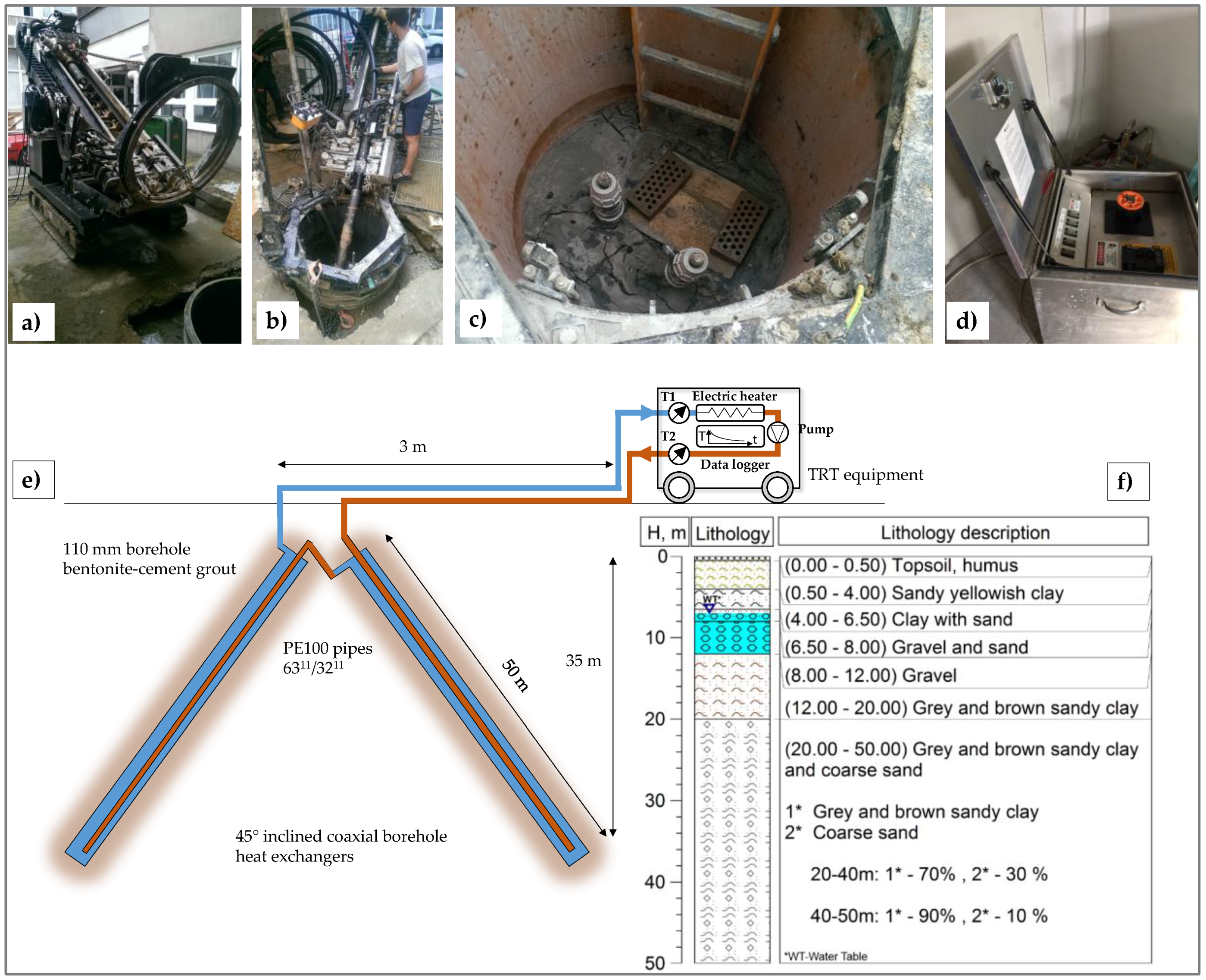
The system comprises two boreholes, each with a length of 50 m, hydraulically connected in series to provide effectively one borehole of 100 m in length. The boreholes were drilled with a standard diameter of 110 mm, and drilling was performed with specialized equipment that allows the drilling angle to be set from 35° to 65°, and in all directions (Figure 5b). 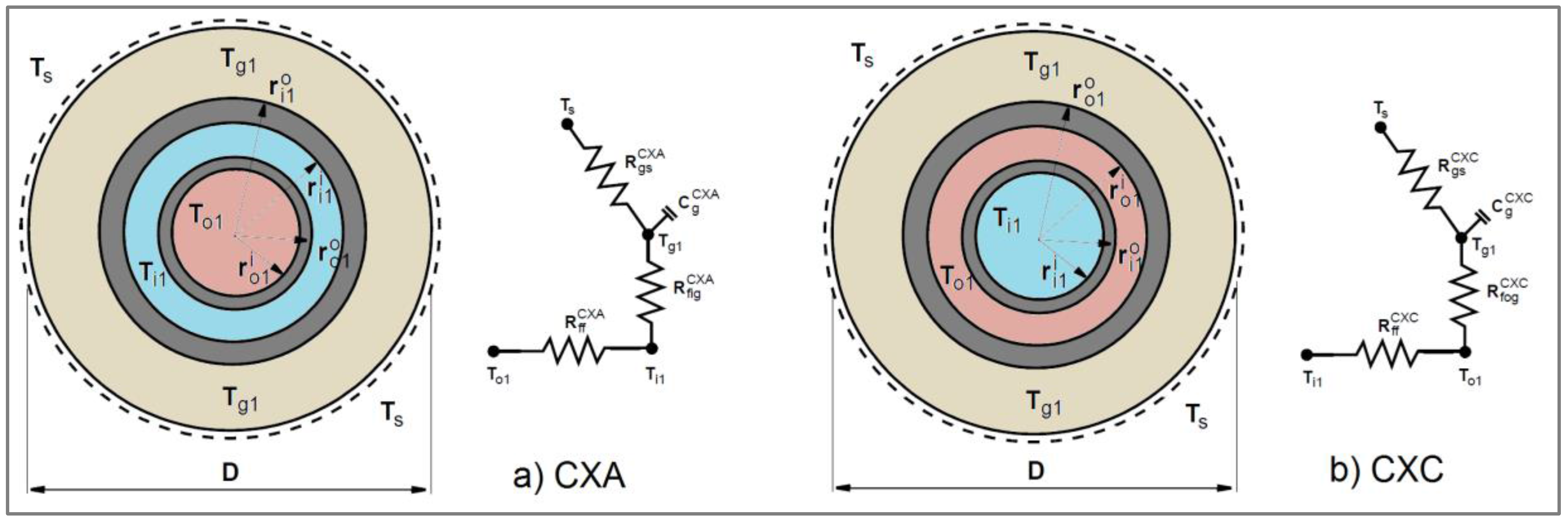Each borehole has an angle of 45°, and these are placed opposite to one another inside a polyethylene shaft with a diameter of 1 m and depth of 1 m (Figure 5c). The coaxial heat exchangers comprise an outer polyethylene pipe of 63 mm with Standard Dimension Ratio of SDR11, while the inner polyethylene pipe is 32 with SDR11. Thermal response testing was conducted on both possible flow arrangements, CXC and CXA setup (see Section 3.4). Cementing with thermally enhanced grout was not possible due to the total losses of material into the high-permeability gravel layer. Therefore, the borehole was cemented with a mixture of water, bentonite and cement, with a somewhat lower thermal conductivity of 1.2 W/m K, measured with the needle probe method.

The detailed geological setting of the location, and the city of Zagreb in general, consists of Middle and Upper Pleistocene sediments, where lateral changes of gravel, silt, sand and clay are frequent, and Holocene sediments that consist of yellow-brown gravel, sand and limestone pebbles. The faculty is located in the northern part of the Zagreb aquifer, just near the outer boundary, with a thin aquifer layer present at a depth of between 6.5 and 12.0 m beneath the surface. The lithological profile, obtained from drilling data, is shown in Figure 5f. The undisturbed ground temperature and geothermal gradient at the Zagreb location were investigated in our previous research [7,23,24,25], which demonstrated a geothermal gradient corresponding to 5.5 °C per 100 m of depth, and an undisturbed ground temperature of approximately 14.5 °C at a depth of 10 m.

As can be seen from Figure 5e, the geometry of the inclined coaxial system implies that the final depth of the boreholes is 35 m beneath the surface. Since aquifer is present in the shallow thin layer, which has a thickness of 5.5 m, the cumulative length of the pipes affected by additional convective heat transfer from groundwater is 16 m out of 100 m in total. Based on regional hydrogeological research data, the hydraulic conductivity of the aquifer near the outer boundary is only 0.3 cm/s; therefore, the convective component of heat transfer was ignored in the thermal response test. In cases of higher hydraulic conductivity, or a thicker groundwater layer in the lithological column, basic hydrogeological interpretation needs to be conducted to determine the Peclet number. In saturated coarse gravel, the Peclet number usually has a value greater than 500, which means that there is a dominant convective heat transfer; while for fine saturated sand, the value is around 1. Silts and clays give values lower than 0.01, which suggests a completely conductive heat transfer [26,27,28].

The measurements on the coaxial heat exchangers were conducted between September 2016 and June 2017, with a Geocube GC500 TRT apparatus (Precision Geothermal LLC, Maple Plain, MN, USA). The equipment has a maximum available power for the electric heaters of 9.0 kW @ 240 V. An internal logger collects 5-min interval data about inlet and outlet fluid temperature, air temperature, flow, voltage and electric current. Sealed temperature sensors (Onset Computer Corporation, Bourne, MA, USA) (resistance temperature detectors—RTD) on inlet and outlet connection have an accuracy of ±0.2 °C from 0 °C to 50 °C.

The testing procedure was organized as a classic TRT heat rejection step with a duration of 96 h, followed each time by a recovery period of an additional 96 h (only circulation). Five different heat steps were used—35, 42, 54, 61 and 71 W/m—for each of the two possible flow setups, CXC and CXA. Ultimately, the total testing time on the coaxial heat exchanger was 192 h for each of the ten different conditions, making for an accumulated 1920 h of data with 5 min logging intervals. After each testing condition, a pause was taken for a duration of seven days, allowing recovery of the ground and the borehole fluid temperature to static initial conditions. Unlike classic 2U-loop vertical heat exchangers with a depth of 100 m, inclined coaxial heat exchangers exploit shallow geothermal sources up to vertical depths of only 35 m. Hence, the initial ground temperature conditions due to different climate seasons are much more affected by the surface air temperature for this kind of installation. Additionally, in practical installations, coaxial heat exchangers are densely radially drilled from a single shaft, causing much more thermal interference between adjacent boreholes in the first few meters of depth.

Table 1. TRT heat step descriptive statistics.

	CXC					CXA
TRT Heat Step, Mean	70.9	61.2	54.5	42.5	35.3	70.8	60.6	53.9	43.0	35.5
Standard Error	0.031	0.024	0.015	0.019	0.016	0.028	0.023	0.026	0.022	0.013
Median	71.0	61.4	54.5	42.6	35.3	70.8	60.7	54.1	43.2	35.5
Mode	72.1	61.6	54.4	43.1	34.7	69.8	60.4	54.2	43.5	35.7
Standard Deviation	1.06	0.81	0.53	0.64	0.56	0.96	0.80	0.88	0.73	0.45
Sample Variance	1.13	0.65	0.28	0.41	0.31	0.91	0.64	0.77	0.54	0.20
Kurtosis	−0.73	−0.29	−0.26	−0.67	−0.92	−0.17	−0.29	−0.70	−0.64	−0.56
Skewness	−0.32	−0.65	−0.12	−0.33	−0.08	−0.39	−0.54	−0.38	−0.49	−0.49
Range	4.77	4.41	2.64	2.94	2.35	5.33	3.97	3.97	3.19	2.24
Minimum	68.3	58.3	53.0	40.7	34.0	67.7	58.3	51.8	41.2	34.1
Maximum	73.1	62.7	55.7	43.7	36.3	73.0	62.2	55.7	44.4	36.4
Sum	81,499	70,671	62,709	48,874	40,579	81,443	69,752	61,999	49,536	40,813
Count	1150	1154	1151	1150	1151	1151	1151	1151	1151	1151
Confidence Level (95.0%)	0.06	0.05	0.03	0.04	0.03	0.06	0.05	0.05	0.04	0.03

presents the results of MS Excel (Supplementary Materials) descriptive statistics related to TRT heating power for each of the ten different heat steps; five for the CXC flow arrangement and five for the CXA arrangement. The acceptable maximum standard deviation for input power is +/−1.5% from the average power level, according to ASHRAE standard 1118-TRP. Furthermore, peak variations must be kept at less than 10% of the average power level. It can be seen from test data that the entirety of the power data fits inside the industry guidelines provided, with the largest deviations seen for the highest power steps, as expected.

Table 2. Air temperature descriptive statistics during TRT.

	CXC					CXA
Mean, TRT Heat Step	70.9	61.2	54.5	42.5	35.3	70.8	60.6	53.9	43.0	35.5
Air Temperature, Mean	10.2	9.1	−1.2	−1.1	21.0	14.4	12.3	14.0	16.2	19.8
Standard Error	0.30	0.29	0.25	0.31	0.29	0.24	0.36	0.29	0.34	0.24
Median	10.7	8.7	−1.3	−0.5	20.2	13.8	13	13.2	16	19.5
Mode	6.0	13.9	−0.1	0.4	18.0	12.4	4.4	11.1	18.8	21.0
Standard Deviation	4.12	4.04	3.47	4.28	4.06	3.35	5.07	4.04	4.78	3.27
Sample Variance	16.9	16.3	12.0	18.3	16.5	11.2	25.7	16.3	22.9	10.7
Kurtosis	−0.71	−1.13	0.77	−0.42	−0.71	−0.34	−0.95	−0.32	−0.63	−0.63
Skewness	0.00	0.05	0.51	−0.29	0.45	0.43	−0.24	0.58	−0.21	0.37
Range	18.2	16	19.6	19.6	16.2	15.4	20	17	19.9	14
Minimum	1.8	0.8	−9.3	−10.1	13.9	7.8	1.8	7.4	4.9	14.1
Maximum	20.0	16.8	10.3	9.5	30.1	23.2	21.8	24.4	24.8	28.1
Sum	1977	1758	−234	−207	4062	2788	2374	2710	3124	3819
Count	193	193	193	193	193	193	193	193	193	193
Confidence Level (95.0%)	0.58	0.57	0.49	0.61	0.58	0.48	0.72	0.57	0.68	0.46

provides descriptive statistics results related to air temperature measurements for a 1-h step. The entire test procedure extended over a six-month period due to there being ~2000 h of testing, in addition to one week of waiting time for the ground to return to initial conditions. Therefore, it could be seen that the mean air temperature data are scattered for each of the heat steps, especially the minimum and maximum values. This also, to some degree, affects the initial temperature conditions for such a shallow geothermal installation, since solar perturbation affects ground up to a depth of 10 m at the test location, and the final depth of the boreholes is 35 m (Figure 5e).

5. Results and Discussion

As explained in Section 4, TRT + recovery period was performed for ten heat steps and two different flow arrangements. For each of the steps, a classic TRT analysis was performed under heat power conditions. Before turning on the electric heaters, the initial borehole temperature was recorded for 30 min of solely fluid circulation. The flow for each of the ten steps was set to 0.42 L/s, and the circulating fluid was pure water. Considering the coaxial pipe arrangement and dimensions (D63^SDR11/D32^SDR11), the volume flow and velocity, the viscosity and density of water, and the pipe roughness, there was a fully developed turbulent regime in both the annular space (Re = 7100) and the column pipe (Re = 23,000).

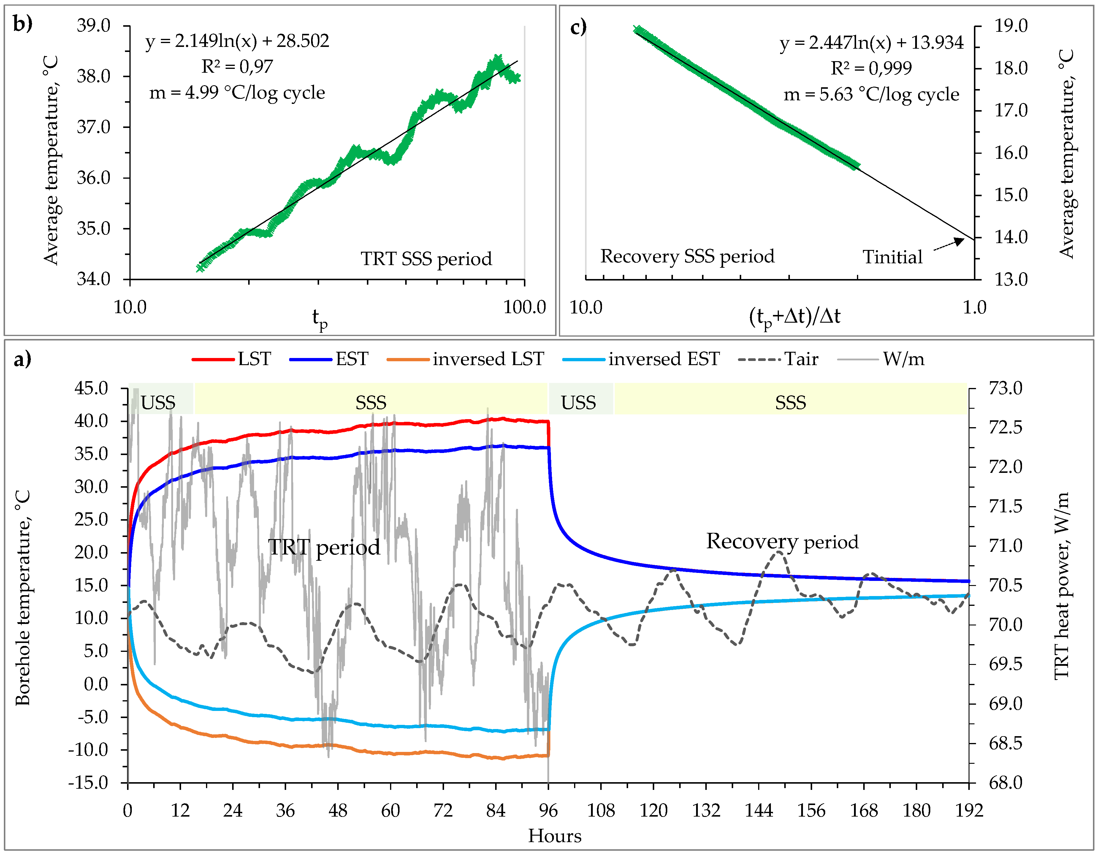
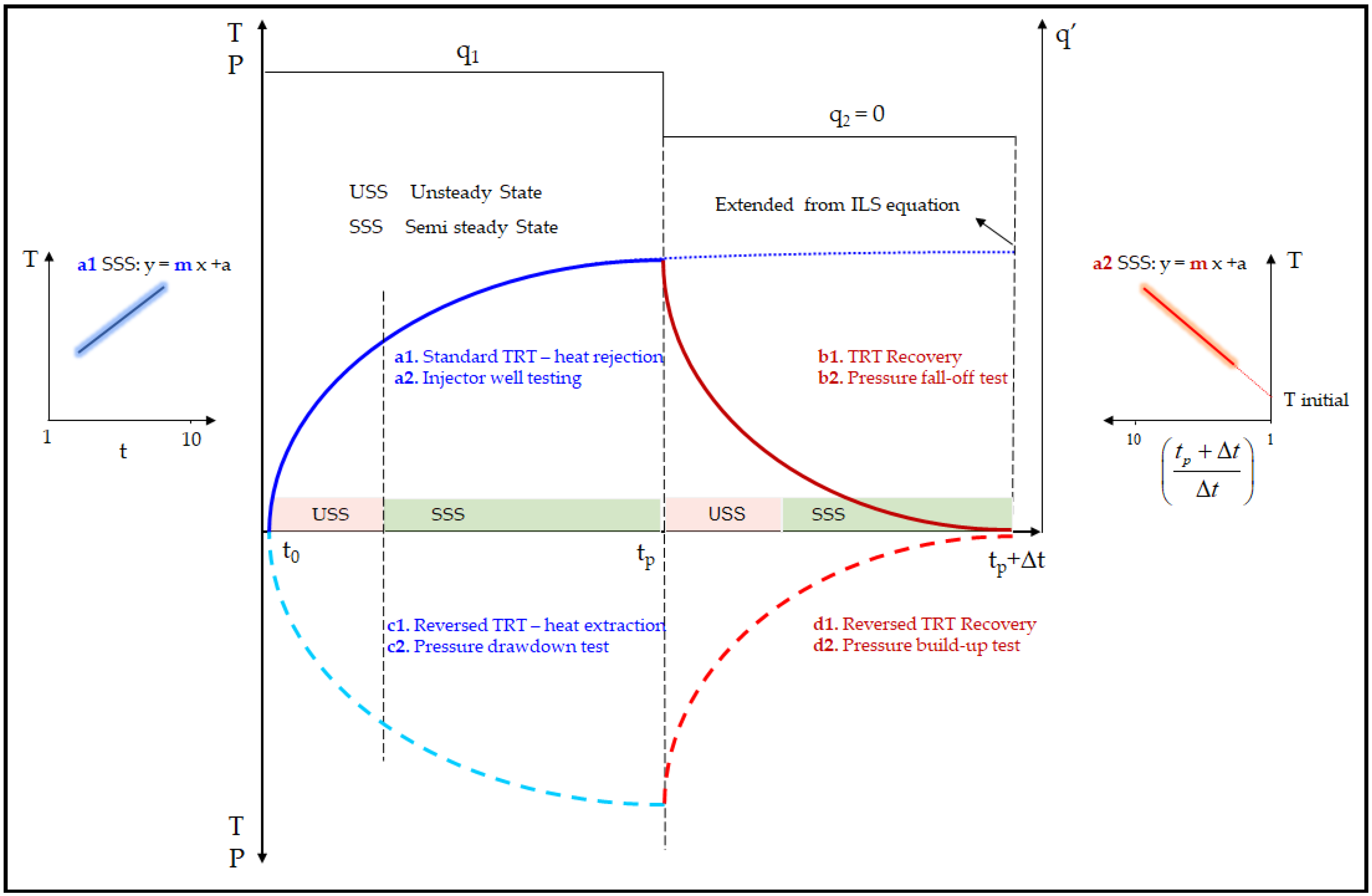
Figure 6a presents the standard analysis for each step, where the entering source temperature (EST), leaving source temperature (LST), and unit heat power is plotted as a function of test time (96 h + 96 h). Since TRT is usually performed based on the principle of heat rejection into the ground, inverse mirror flow/return curves were charted to represent the cycle in which the heat pump was in heating mode (subcooling the ground). This approach better represents the working conditions during the extraction of heat from the ground (the heat pump heating cycle, for example).

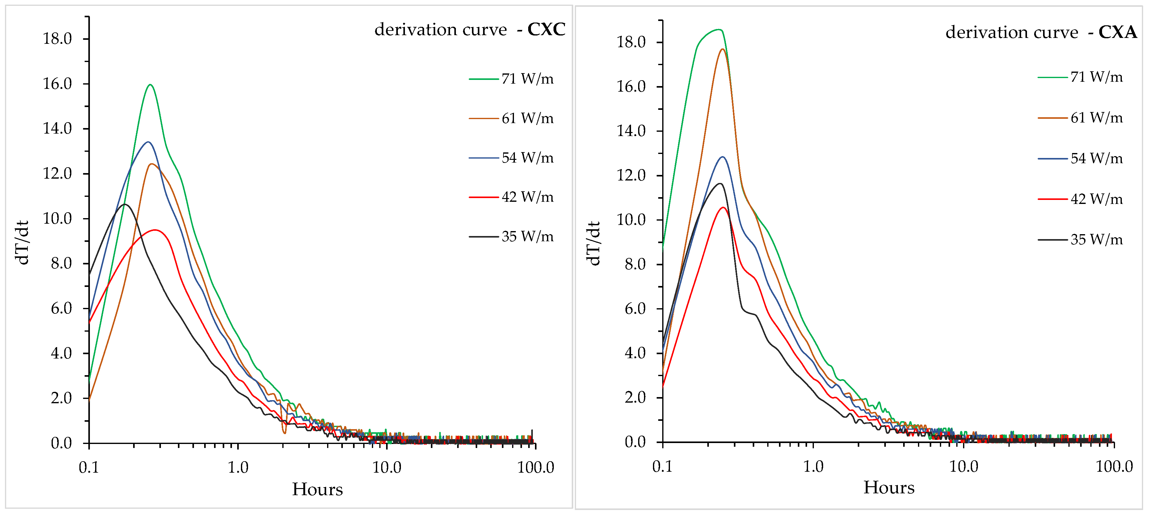
To determine the effective ground thermal conductivity for each of the ten analyzed cases, the emersion time of the semi-steady-state heat flow had to be identified from the initial unsteady state. Based on the theory presented in Section 3.3, derivation curves were created for each of the ten TRT periods. The results are shown in Figure 7. It is evident that a semi-steady state appears after the ~10th h of investigation, where the change of the temperature per unit time reaches 0.25 °C per 5-min time step. Since most of the lithology column is made out of damp clay (except thin saturated gravel near surface), the effective thermal diffusivity, according to catalogue soil data, could be anywhere from 0.030 to 0.060 m²/d, depending on the moisture content. As a reasonable estimation, we assumed a value of 0.050 m²/d for further analysis. If the appearance of SS-state is deduced from the standardized equation by Mogensen presented in Section 3.3, then the corresponding time would be 7.5 h for a borehole diameter of 110 mm. To achieve maximum accuracy and nullify transient effects, the ground thermal conductivities were derived from intervals of 15–96 h for all test conditions in the TRT period and recovery period.

In Figure 6a,b, the procedure of deriving ground thermal conductivities can be seen. For the case of the TRT period, semi-log axes were used, and borehole T_avg vs. t_p was plotted for the Semi-Steady State or SSS interval. As stated by Equation (10), since a semi-log plot is used, there is the need to determine the change of temperature for a one-log cycle of time (m), and then calculate the effective ground conductivity. The same result could be obtained by using the standardized principle of plotting T_avg vs. ln(t_p) on a normal graph, and then using Equation (9) and the slope of the line κ.

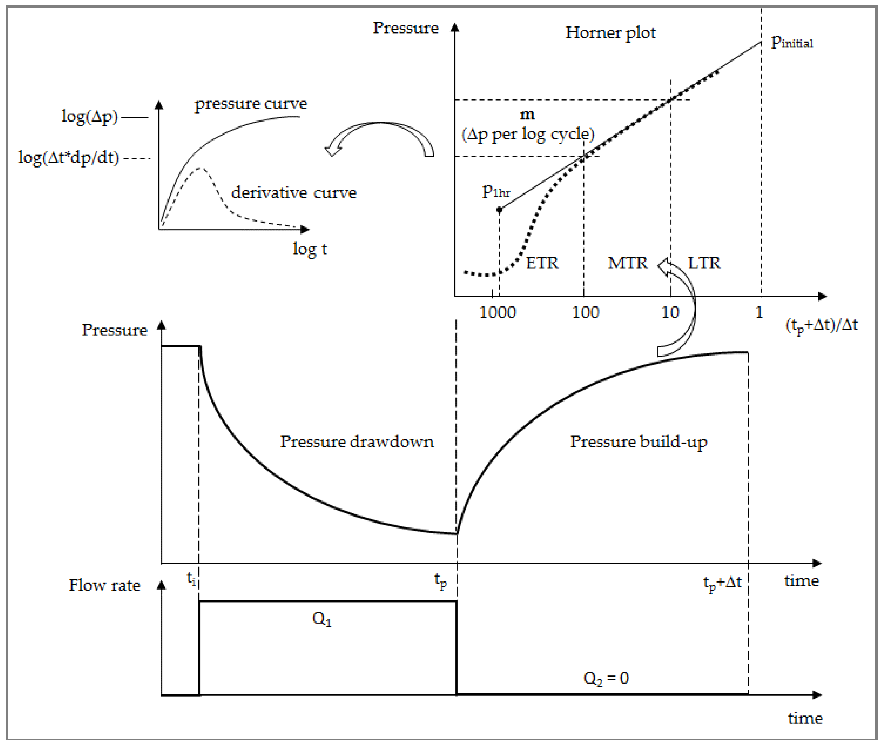
When analyzing the recovery period, a slightly different approach has to be used, as explained in Section 3.2. A reversed semi-log graph has to be used, and T_avg is plotted vs. (t_p + Δt)/Δt, as shown by Figure 6c. Effective ground thermal conductivity is then derived from Equation (17) by knowing the log slope m, just like in the case for a standard TRT period. When the temperature recovery line is extended until (t_p + Δt)/Δt = 1, initial conditions—i.e., undisturbed ground temperature—are reached. 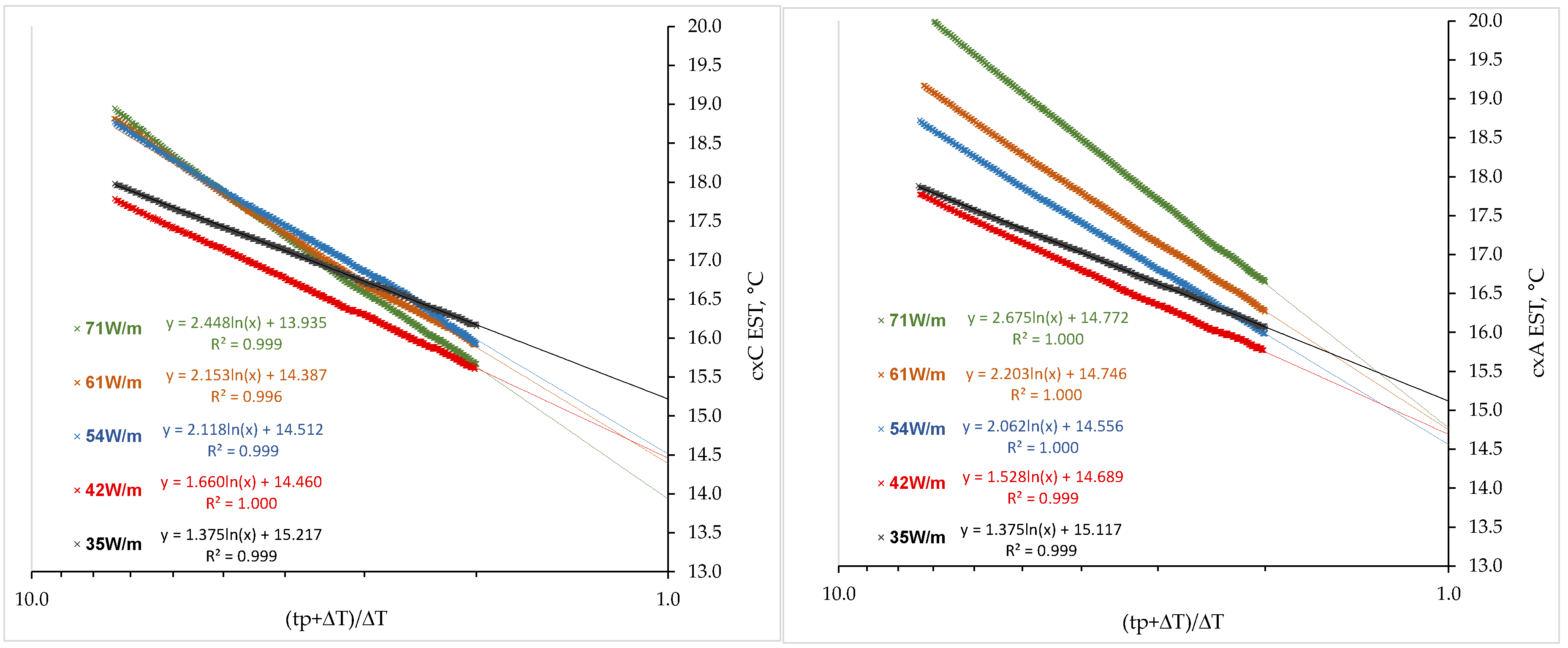Figure 8 shows the entire Horner’s procedure for all ten heat step conditions. It is important to note that testing times of 15–96 h were used in this analysis, in order to nullify transient effects, just like in the case of TRT. When extending the data trendline until (t_p + Δt)/Δt = 1, it can be seen that the initial temperature value ranges between 14.0 °C and 15.2 °C. As mentioned before, the reason for this effect is the shallow installation of the coaxial system with a final depth of 35 m, while solar energy perturbation penetrates to a depth of 10 m. Therefore, the initial condition values are somewhat dependent on the climate and season in which the measurements are taking place.

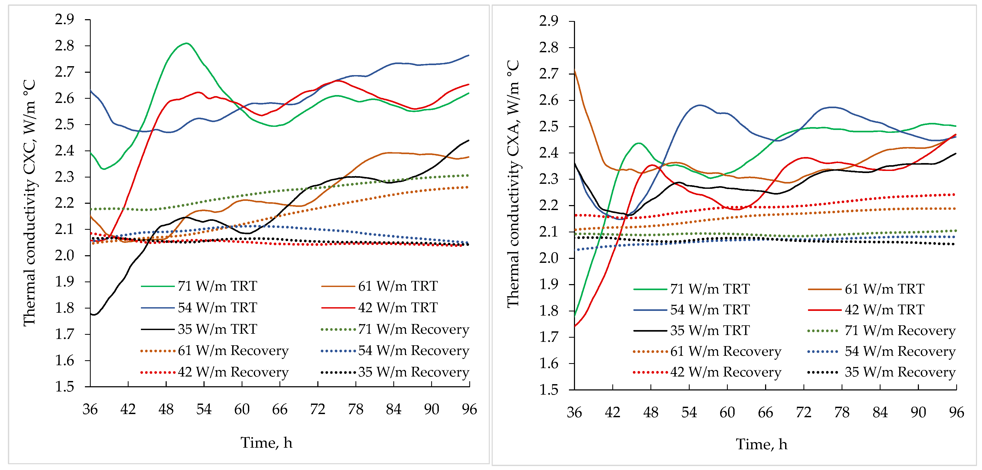
Since the total duration of TRT is not strictly defined, only the minimum time is required, as explained in Section 2; in practical field testing, this always leads to a certain degree of analysis error. Since the final duration is arbitrarily chosen by the TRT operator, different test times could lead to quite different thermal conductivities. Figure 9 shows an analysis of thermal conductivity values with variable test duration between 36 and 96 h. When looking at the thick lines on both graphs, for CXC and CXA, it can be seen that choosing different TRT periods could lead to as much as a 20% difference in the final result. From a standpoint of modelling geothermal heat pumps with multiple boreholes, such discrepancies could have a significant impact on oversizing or undersizing the geoexchange system, and on technoeconomical benefit.

Such a difference in results is influenced primarily by two factors: fluctuations of voltage in the public electrical grid, which is the usual method of powering TRT; and interferences between the surface equipment and air temperature, especially during the winter months. As explained in Section 2, fluctuations in voltage from the public grid are regularly seen to be following recognizable patterns in a 24-h cycle, depending on the specific demand during the day and night. Therefore, to at least try to minimize the effects of this on the development of line slope, as shown in Figure 6b, TRT duration should follow a 24 h multiplication factor (i.e., 48, 72, 96 h or 36, 60, 84 h). The other major concern is that of ambient temperature interfering with the TRT equipment and header pipes. As seen from Figure 5e, we used a header pipe length of 3 m from the borehole shaft to the TRT equipment in order to purposely magnify this effect, although the entire setup was properly insulated with 12 mm of caoutchouc rubber insulation. The effect of this could be seen in terms of the higher conductivity deviation for the CXC, as opposed to the CXA flow arrangement. Theoretically, flow direction arrangement does not have an impact on the conductivity measurement procedure, but rather on borehole resistance; nevertheless, the CXC tests were carried out during autumn/winter months, and the CXA during the spring months. The data shown in Table 2 conclusively suggest this claim, explaining the reason for the higher measured thermal conductivity for the CXC compared to the CXA tests.

Prolonging the TRT procedure by conducting additional recovery period, and using Horner’s method to interpret the data, could lead to higher accuracy in approaching the actual ground thermal conductivity. This is clearly seen from Figure 9, where thermal conductivity obtained by Horner’s method from the recovery period gives more symmetrical results, for both the CXC and CXA setups. This is explained by the fact that the recorded data is smooth, since there is no heat power applied (coefficient of determination from 0.996 to 1.0, as seen from Figure 8), and the fact that during the winter months, the interference heat flux between ambient and TRT equipment is lower, due to the lower temperature difference between the air temperature and the fluid temperature. The entire analysis presented with the two-step TRT principle could provide geothermal engineers a more precise method for qualitatively interpreting field data.

Furthermore, as stated in Section 3.4, both the TRT period and the recovery period could be used to determine the equivalent borehole resistance or skin effect, an equally important parameter for the efficient design of geoexchange systems. By applying Equations (24) and (25) to TRT data for each heat step, and Equation (27) for Horner’s method on the recovery period, the following values were obtained, as shown in

Table 3. Obtained data from analysis of TRT and recovery periods.

Flow Setup	CXC					CXA
TRT Heat Step, Mean	70.9	61.2	54.5	42.5	35.3	70.8	60.6	53.9	43.0	35.5
Thermal conductivity @96 h, W/m °C during TRT period	2.62	2.38	2.72	2.65	2.44	2.50	2.47	2.46	2.47	2.40
Thermal conductivity @96 h, W/m °C during Recovery period	2.25	2.26	2.05	2.04	2.04	2.11	2.19	2.08	2.24	2.05
Initial temperature, TRT circulation, °C	14.6	14.7	14.8	14.6	14.8	14.7	14.7	14.7	14.7	14.7
EST after 96 h of TRT, °C	36.0	33.7	32.0	28.1	26.6	37.8	33.9	31.9	28.2	26.5
EST after 96 h of Recovery period, °C	15.7	15.9	15.9	15.6	16.2	16.7	16.3	16.0	15.7	16.1
Initial temperature, Horner, °C	13.9	14.4	14.5	14.5	15.2	14.8	14.7	14.5	14.7	15.1
Borehole resistance, Horner, m °C/W	0.138	0.138	0.127	0.126	0.129	0.135	0.133	0.131	0.135	0.128
m slope, Horner, °C/log cycle	5.6	5.0	4.9	3.8	3.2	6.2	5.1	4.7	3.5	3.2
skin factor, Horner, °C	2.0	2.0	1.6	1.6	1.7	1.8	1.8	1.7	1.9	1.7
T1 h, Horner, °C	25.1	24.2	24.2	22.0	21.5	27.0	24.8	24.0	21.7	21.4
Tp, Horner, °C	36.0	33.6	32.0	28.1	26.6	37.7	33.9	31.9	28.2	26.5

. It can be seen that the CXA flow arrangement generally shows a higher skin effect or equivalent borehole heat resistance (approximately +5%), which is in line with our previous research in this field [23], in which the borehole resistances of inclined coaxial and vertical 2U-loop heat exchangers were compared.

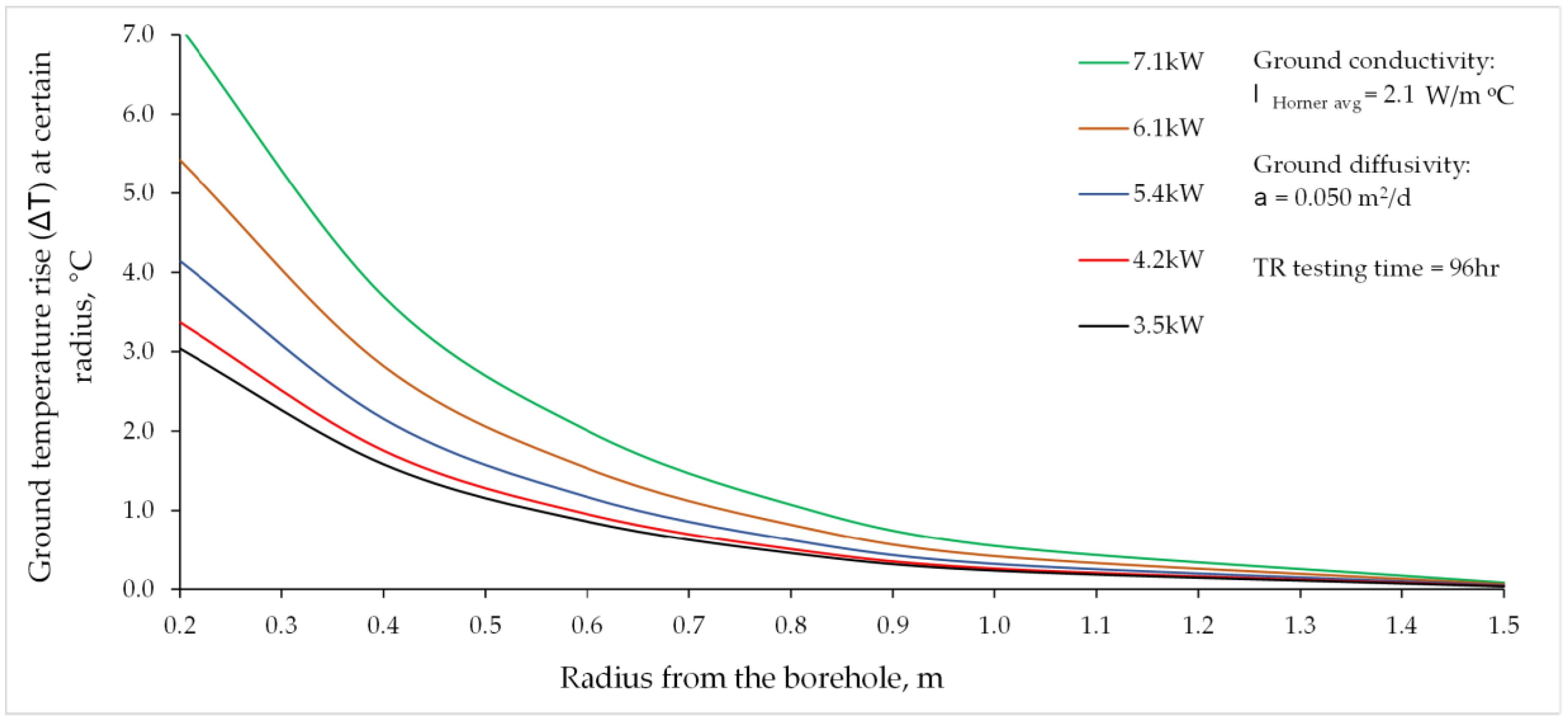
Figure 10 shows the analysis of the ground temperature change at a certain radius away from the borehole after a Thermal Response Test time of 72 h. Temperature change was calculated with the infinite line source solution presented in a Section 3.1 for the case of five heat rejection steps. Due to its having more equable values, the ground effective thermal conductivity was set as the average of all ten measurements conducted by the Horner method in the recovery test period (Table 3). As mentioned in Section 4, densely drilled and installed inclined coaxial heat exchangers from a single shaft are prone to thermal interference between adjacent pipes for the first few meters of depth. As seen in Figure 10, for a TR test time of 72 h, these interferences could be ignored, as temperature change is negligible for a radius larger than 1.0 m. As shown in Figure 5, the two inclined boreholes were closer than this value only very near the surface, since drilling was conducted at a 45° angle and in opposite directions. This result also suggests that the infinite line source solution is reasonable to use for two boreholes connected in series.

Discrepancies between the thermal conductivity obtained for the TRT period and the recovery period were rather high (TRT analysis showed 10–20% higher values than the Horner method), as can be seen from Table 3 and Figure 9. We have already explained the causes for this phenomenon, but using simple statistical analysis, such as sum of squares of difference, could provide knowledge of exactly which thermal conductivity coefficients are of statistical significance. The Sum of Squares or simply variation (SUMXMY2 function in MS Excel $=\Sigma {\left(x-y\right)}^2$) is a statistical technique used in regression analysis to determine the dispersion of data points. In a regression analysis, the goal is to determine how well a data series (in this case, measured EST) can be fitted to a function that might help to explain how the data series was generated (in this case, ILS with Ei function with two different thermal conductivities). The sum of squares is used as a mathematical way of finding the function that best fits (varies least) from the measured data.

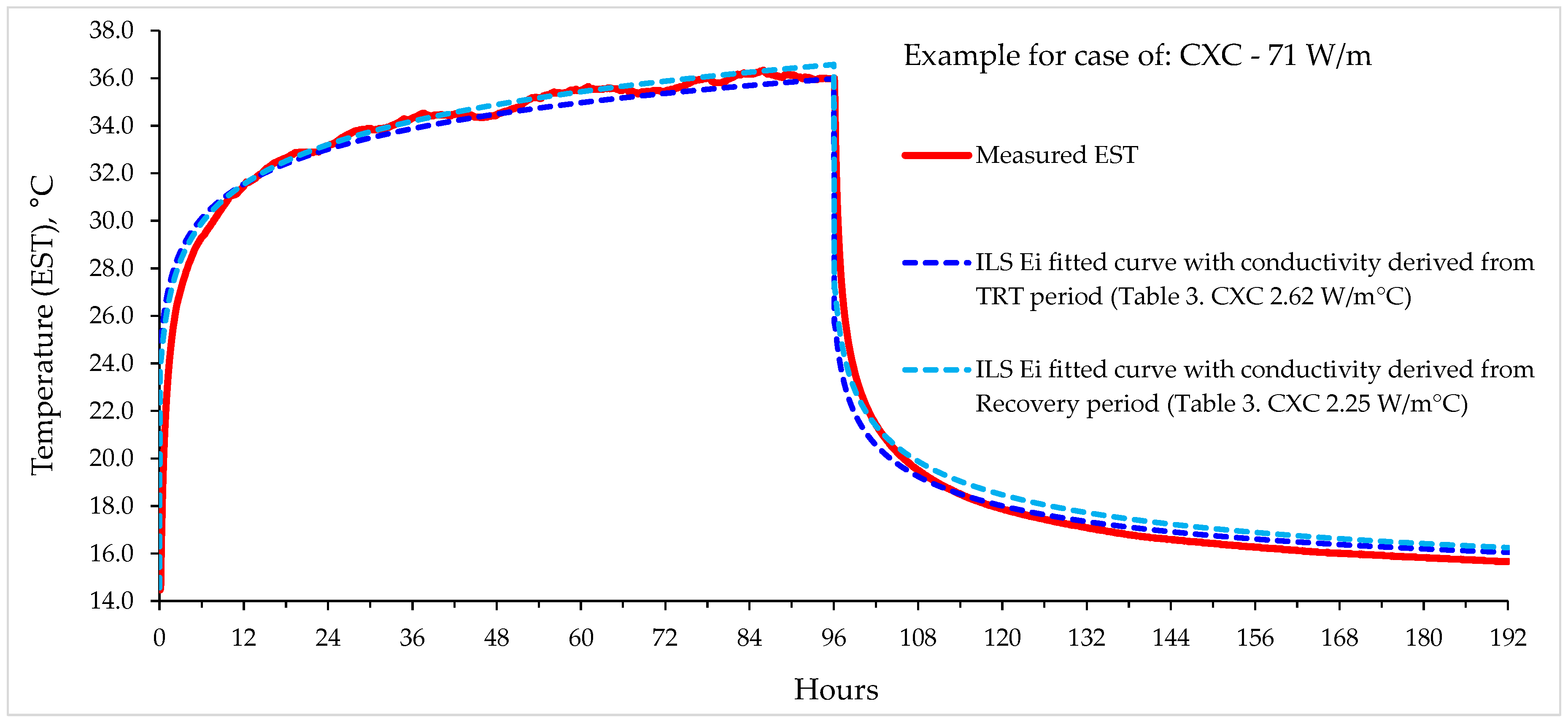
The procedure was carried out for every heat step separately, with two obtained values for the thermal conductivity factor: one from the TRT period and one from the recovery period. Then, the entire curve was fitted with Equation (28) for the first step period, and Equation (29) for the second step period. An example is shown in Figure 11 for the case of CXC and 71 W/m. The dark blue dotted line is an ILS exponential integral function curve that takes into account a thermal conductivity value of 2.62 W/m °C (obtained during TRT), while the light blue dotted line is for a thermal conductivity value of 2.25 W/m °C (obtained during the recovery period). The purpose of this procedure was to find which thermal conductivity value better described the recorded temperature during the test for both periods (TRT 96 h + Recovery 96 h).

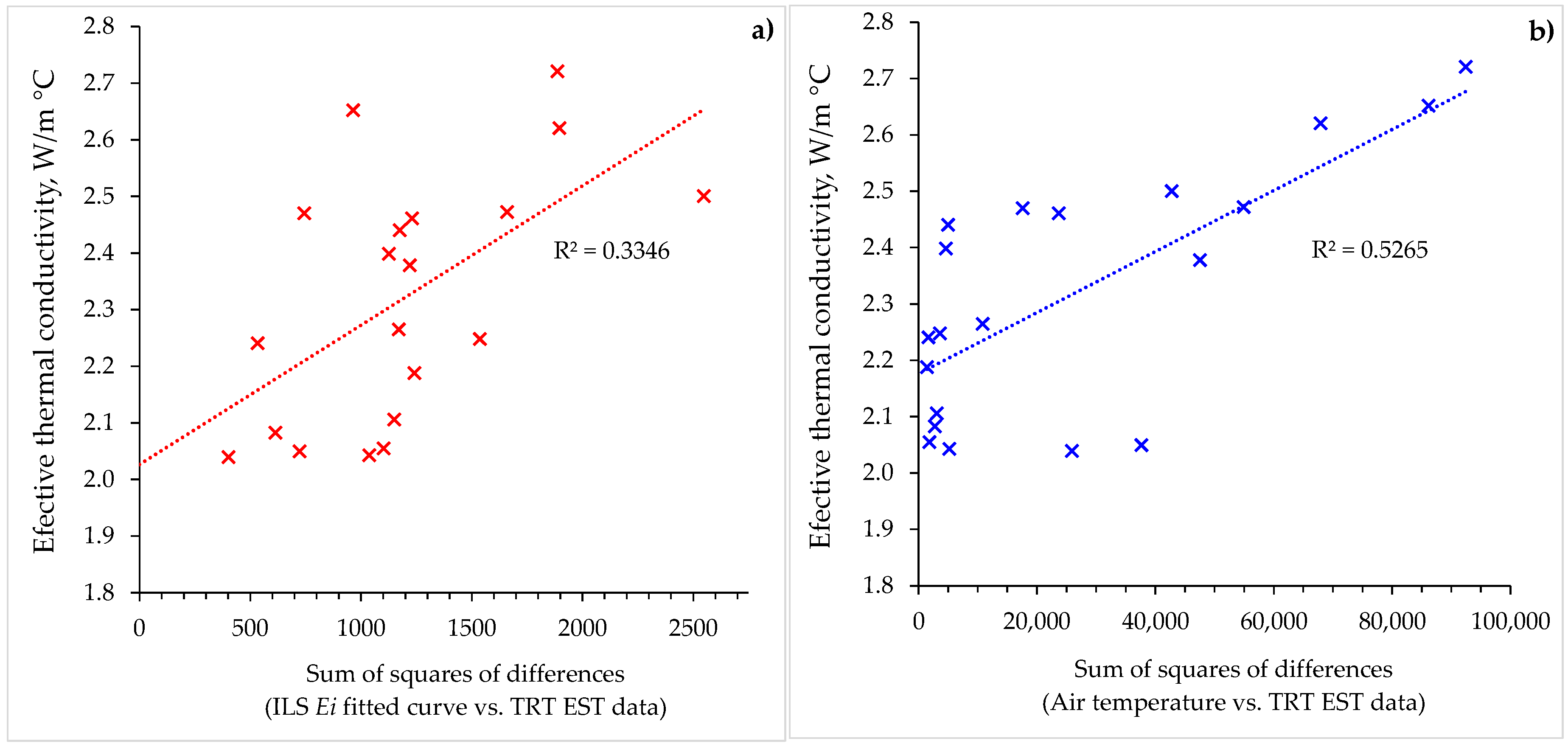
In this way, a total of 20 points were obtained on the basis of the same principle as that presented in Figure 11; each data set was fitted with two Ei function curves with two different thermal conductivities. The results are presented in Figure 12a.

The same kind of variation analysis was performed with the EST hourly measured data and hourly air temperatures for each period (TRT or recovery) and heat step. The assumption was that the measurements with higher differences between the air temperature and the circulating fluid temperature would have higher thermal interferences and, consequently, higher degrees of error. This is especially true for this kind of TRT setup, where equipment is placed 3 m from the borehole (Figure 5e). Some thermal interference phenomena are to be expected in such cases, although the surface pipes are insulated. The results are shown in Figure 12b, in which the associated thermal conductivities are plotted against the sum of squares of differences between EST and T_air. Since the air temperature was recorded for the entire ~2000 h of measurement, the hypothesis is that climate interference would be zero if the air temperature were the same value as the current EST of the borehole fluid. The higher the temperature difference between the air temperature and the EST of the borehole fluid at any moment, the higher the interference would be on the TRT ground conductivity analysis, since a certain heat transfer would take place between the environment and the surface collector pipes and equipment.

Both statistical analyses in Figure 12a,b shows similar trendlines, where for a value of SUMXMY2 = 0, the ground thermal conductivity coefficient is in the range 2.0–2.2 W/m K. This is, in fact, a value very near the average of the ground thermal conductivities obtained by ten tests conducted in the recovery period (l_{horner avg} = 2.13 W/m °C), as seen in Figure 9.

As previously stated, the soil thermal diffusivity was reasonably estimated based on the known geological column and the obtained drilling samples. The soil thermal diffusivity termaffects the value of the calculated borehole resistance or skin term, due to the interconnectivity of the two variables in solutions presented for the diffusivity equations for cases of infinite medium and line source well. The conducted sum of squares of differences analysis, as presented in Figure 11 and Figure 12, would not be affected by altering the initially assumed soil thermal diffusivity term. Changing this value, in a range of 0.03–0.06 m²/d as expected for clays, would only change the resistivity/skin term. Inverse analysis could also be conducted, by calculating the thermal resistance term based on a known well geometry and material thermodynamic characteristics, and determining the soil thermal diffusivity term using ILS equations. However, practical geometry and the completion of the borehole heat exchanger is often different from the one assumed in this project. This problem is often related to misaligned pipes in the wellbore (especially in inclined coaxial systems) and the quality of the grouting (especially perfect adherence of grout and pipe). Soil diffusivity could be more precisely determined by laboratory measurements of undisturbed soil samples, by determining density, specific heat capacity and conductivity.

Therefore, the presented results confirm the hypothesis of this paper that a prolonged TRT should be conducted wherever possible, since it provides a higher certainty of the real ground thermal conductivity value.

6. Conclusions

Ground thermal conductivity and borehole skin factor, obtained from TRT measurements, are a prerequisite for optimized design of the borehole heat exchanger field. Such systems are, in practice, often unnecessarily oversized, as a result of the insecurity factor, or undersized, as a result of poor engineering design and lack of understanding of ground properties. In both cases, this negatively reflects on the economic viability of the geothermal project itself. From this perspective, longer and more advanced ground thermal response measurements are more cost-effective, as they ensure the longevity of the system and the knowledge of the borehole temperature evolution throughout the entire year.

Therefore, practical borehole heat exchanger field tests should always consist of a classic TRT test and a corresponding recovery test of the same duration. Interpreting the temperature recovery period with the Horner technique, derived from petroleum well testing experiences, elevates certainty that the obtained ground thermal conductivity coefficient is as close as possible to the real value. Furthermore, such a procedure minimizes the negative effects of electric grid voltage fluctuations and interferences from the ambient climate when performing classic TR tests.

References

1. American Society of Heating, Refrigerating and Air-Conditioning Engineers (ASHRAE). ASHRAE Handbook—HVAC Applications; American Society of Heating, Refrigerating and Air-Conditioning Engineers: Atlanta, GA, USA, 2007; Chapter 34. [Google Scholar]
2. Bujok, P.; Grycz, D.; Klempa, M.; Kunz, A.; Porzer, M.; Pytlik, A.; Rozehnal, Z.; Vojčinák, P. Assessment of the influence of shortening the duration of TRT (thermal response test) on the precision of measured values. Energy 2014, 64, 120–129. [Google Scholar] [CrossRef] [Green Version]
3. Bandos, T.V.; Montero, Á.; Fernández de Córdoba, P.; Urchueguía, J.F. Improving parameter estimates obtained from thermal response test: Effect of ambient temperature variation. Geothermics 2011, 40, 263–270. [Google Scholar] [CrossRef]
4. Borinaga-Trevino, R.; Norambuena-Contreras, J.; Castro-Fresno, D. How to correct the ambient temperature influence of the thermal response test results. Appl. Therm. Eng. 2015, 82, 39–47. [Google Scholar] [CrossRef]
5. Signorelli, S.; Bassetti, S.; Pahud, D.; Kohl, T. Numerical evaluation of thermal response tests. Geothermics 2007, 36, 141–166. [Google Scholar] [CrossRef]
6. Kurevija, T.; Macenić, M.; Strpić, K. Steady state heat rejection rates for coaxial borehole heat exchanger during passive and active cooling determined with the novel thermal response test method. Rud. Geol. Naftni Zb. 2018, 33, 1–17. [Google Scholar] [CrossRef]
7. Gehlin, S. Thermal Response Test: Method Development and Evaluation. Ph.D. Thesis, Luleå University of Technology, Luleå, Sweden, 2002. [Google Scholar]
8. Badenes, B.; Pla, M.Á.M.; Lemus-Zúñiga, L.G.; Mauleón, B.S.; Urchueguía, J.F. On the Influence of Operational and Control Parameters in Thermal Response Testing of Borehole Heat Exchangers. Energies 2017, 10, 1328. [Google Scholar] [CrossRef]
9. Wright, A.; Firth, S. The nature of domestic electricity-loads and effects of time averaging on statistics an on-site generation calculations. Appl. Energy 2007, 89, 389–403. [Google Scholar] [CrossRef] [Green Version]
10. Witte, H.J.L. Error analysis of thermal response test. Appl. Energy 2013, 109, 302–311. [Google Scholar] [CrossRef]
11. Raymond, J.; Therrien, R.; Gosselin, L.; Lefebvre, R. A review of thermal response test analysis using pumping test concepts. Ground Water 2011, 49, 932–945. [Google Scholar] [CrossRef] [PubMed]
12. Carslaw, H.S.; Jaeger, J.C. Conduction of Heat in Solids; Claremore Press: Oxford, UK, 1946; ISBN 978-0198533689. [Google Scholar]
13. Ingersoll, L.R.; Zobel, O.J.; Ingersoll, A.C. Heat Conduction with Engineering, Geological and other Applications; McGraw-Hill: New York, NY, USA, 1954; p. 325. [Google Scholar]
14. Lee, J. Well Testing, 1st ed.; Society of Petroleum Engineers of AIME: New York, NY, USA, 1982; pp. 1–71. ISBN 0-89520-317-0. [Google Scholar]
15. Horner, D.R. Pressure Buildup in Wells. In Proceedings of the Third World petroleum Congress, The Hague, The Netherlands, 28 May 28–6 June 1951. [Google Scholar]
16. Eskilson, P. Thermal Analysis of Heat Extraction Boreholes. Ph.D. Thesis, University of Lund, Lund, Sweden, 1987. [Google Scholar]
17. Conti, P. Dimensionless Maps for the Validity of Analytical Ground Heat Transfer Models for GSHP Applications. Energies 2016, 9, 890. [Google Scholar] [CrossRef]
18. Mogensen, P. Fluid to duct wall heat transfer in duct system heat storage. In Proceedings of the International Conference on Surface Heat Transfer in Theory and Practice, Stockholm, Sweden, 6–8 June 1983; pp. 652–657. [Google Scholar]
19. Al-Khoury, R.; Bonnier, P.G.; Brinkgreve, R.B.J. Efficient finite element formulation for geothermal heating systems. Part I: Steady state. Int. J. Numer. Methods Eng. 2005, 63, 988–1013. [Google Scholar] [CrossRef]
20. Diersch, H.-J.G.; Bauer, D.; Heidemann, W.; Rühaak, W.; Schätzl, P. Finite element formulation for borehole heat exchangers: Part 1. Fundamentals. Comput. Geosci. 2011, 37, 1122–1135. [Google Scholar] [CrossRef]
21. Matthews, C.S.; Russell, D.G. Pressure Buildup and Flow Tests in Wells, Society of Petroleum Engineers of AIME; Henry L. Doherty Memorial Fund of AIME: New York, NY, USA, 1967; ISBN 978-0-89520-200-0. [Google Scholar]
22. Van Everdingen, A.F. The skin effect and its influence on the productive capacity of a well. J. Pet. Technol. 1953, 5, 171–176. [Google Scholar] [CrossRef]
23. Kurevija, T.; Strpić, K. Hydraulic and thermogeological design differences between two-loop vertical and inclined coaxial borehole heat exchangers. Renew. Energy 2018, 117, 314–323. [Google Scholar] [CrossRef]
24. Kurevija, T.; Vulin, D.; Macenić, M. Impact of geothermal gradient on ground source heat pump system modeling. Rud. Geol. Naftni Zb. 2014, 28, 39–45. [Google Scholar]
25. Kurevija, T.; Vulin, D. Determining undisturbed ground temperature as part of shallow geothermal resources assessment. Rud. Geol. Naftni Zb. 2010, 22, 27–36. [Google Scholar]
26. Domenico, P.A.; Schwartz, F.W. Physical and Chemical Hydrogeology; John Wiley & Sons: New York, NY, USA, 1990. [Google Scholar]
27. Diao, N.; Li, Q.; Fang, Z. Heat transfer in ground heat exchangers with groundwater advection. Int. J. Therm. Sci. 2004, 43, 1203–1211. [Google Scholar] [CrossRef]
28. Conti, P.; Testi, D.; Grassi, W. Transient forced convection from an infinite cylindrical heat source in a saturated Darcian porous medium. Int. J. Heat Mass Transf. 2018, 117C, 154–166. [Google Scholar] [CrossRef]
Figure 1. Typical plot of pressure response during well testing and application of Horner’s method.
Energies 11 00366 g001
Figure 2. Display of corresponding behavior of pressure/temperature during different types of well tests/thermal response tests.
Energies 11 00366 g002
Figure 3. Determination of semi-steady-state heat flow period via the derivation curve technique.
Energies 11 00366 g003
Figure 4. Components of borehole thermal resistance for (a) the CXA arrangement; and (b) the CXC arrangement.
Energies 11 00366 g004
Figure 5. Test site setup: (a) Borehole drilling equipment; (b) Inserting coaxial borehole heat exchanger; (c) Heat exchanger shaft; (d) TRT equipment; (e) Schematics of testing site; (f) Lithology description.
Energies 11 00366 g005
Figure 6. Example of two-step TRT analysis carried out for each heat power condition (CXC 71 W/m presented here); (a) Recorded borehole and air temperatures and unit heat power; (b) Determination of conductivity from TRT period; (c) Determination of conductivity by Horner’s method from recovery period.
Energies 11 00366 g006
Figure 7. EST derivation curves for CXA and CXC flow arrangement and each TRT heat step.
Energies 11 00366 g007
Figure 8. Horner’s semi-log method for determining ground thermal conductivity applied to a TRT recovery period for each heat power step and flow regime.
Energies 11 00366 g008
Figure 9. Results of the ground thermal conductivity values obtained for classic TRT and recovery period as a function of variable test time 36–96 h.
Energies 11 00366 g009
Figure 10. Ground temperature rise at a certain radius from the borehole for five different TRT heat steps.
Energies 11 00366 g010
Figure 11. Example of fitting measured EST data with the infinite line source equation and two different values of thermal conductivity (the first obtained from the TRT period, and the second from the recovery period) for a case of 71 W/m and CXC setup.
Energies 11 00366 g011
Figure 12. Results of sum of squares of differences analysis: (a) SUMXMY2 between ILS fitted curve and EST measured data; (b) SUMXMY2 between air temperature and EST measured data.
Energies 11 00366 g012