Comparative Study of Different Methods for Estimating Weibull Parameters: A Case Study on Jeju Island, South Korea

1
Multidisciplinary Graduate School Program for Wind Energy, Graduate School, Jeju National University, 102 Jejudaehakro, Jeju 63243, Korea
2
Faculty of Wind Energy Engineering, Graduate School, Jeju National University, 102 Jejudaehakro, Jeju 63243, Korea
3
Department of Mechanical Engineering, College of Engineering, Jeju National University, 102 Jejudaehakro, Jeju 63243, Korea
*
Author to whom correspondence should be addressed.
Energies 2018, 11(2), 356; https://doi.org/10.3390/en11020356
Submission received: 12 January 2018
/
Revised: 27 January 2018
/
Accepted: 31 January 2018
/
Published: 3 February 2018
(This article belongs to the Section L: Energy Sources)
Abstract
:On Jeju Island, South Korea, an investigation was conducted to determine the best method for estimating Weibull parameters. Six methods commonly used in many fields of the wind energy industry were reviewed: the empirical, moment, graphical, energy pattern factor, maximum likelihood, and modified maximum likelihood methods. In order to improve the reliability of a research result, five-year actual wind speed data taken from nine sites with various topographical conditions were used for the estimation. Furthermore, the effect of various topographical conditions on the accuracy of the methods was analyzed and 10 bin interval types were applied to determine the most appropriate bin interval based on their performances. Weibull distributions that were estimated using these methods were compared with the observed wind speed distribution. Then the accuracy of each method was evaluated using four accuracy tests. The results showed that of the six methods, the moment method had the best performance regardless of topographical conditions, while the graphical method performed the worst. Additionally, topographical conditions did not affect the accuracy ranking of the methods for estimating the Weibull parameters, while an increase of terrain complexity resulted in an increase of discrepancy between the estimated Weibull distribution and the frequency of the observed wind speed data. In addition, the choice in bin interval greatly affected the accuracy of the graphical method while it did not depend on the accuracy of the modified maximum likelihood method.
1. Introduction
Demand for renewable energy increases due to a number of environmental factors such as climate change, a limited supply of fossil fuels, acid rain, and so on. Among renewable energies, wind is one of the most popular and promising energy sources. The total capacity of global wind power was 486.8 GW by the end of 2016 representing cumulative market growth of 12% [1]. The total capacity of wind power in South Korea was 1031 MW by the end of 2016 of which Jeju Island represented about 25.9%. Offshore capacity in South Korea was 35 MW at the end of 2016 and all offshore projects were located off the coast of Jeju Island [2].
Weibull distribution is a suitable model for wind speed frequency distribution and it has been widely used in many fields of the wind energy industry. In particular, it provides a convenient representation of potential wind energy, and it is used to assess the economic feasibility of a potential wind farm [3,4,5]. Thus, it is important to determine how closely the data from Weibull distribution estimates match data from actual wind speed distribution. Weibull distribution is a two-parameter function and these parameters—named the shape parameter, k, and the scale parameter, c—determine the form and characteristics of distribution [6,7,8,9]. In addition, two-component Weibull mixtures have been developed to improve the performance under the conditions of bimodal wind speed distribution [10,11,12].
Various methods have been developed to estimate Weibull parameters using observed wind data. Justus et al. [13] suggested an empirical method, which can be calculated using the average and the standard deviation of wind speed data, to provide a practical solution. Stevens and Smulders [14] suggested the maximum likelihood method (MLM), which is based on numerical iteration. Deaves and Lines [15] presented the graphical method, which uses a linear least-squares regression. Akdag and Dinler [16] presented the energy pattern factor method, which was reportedly suitable for calculating power density and average wind speed.
Furthermore, comparative studies of these methods have been conducted using statistical analysis. Seguro and Lambert [17] estimated Weibull parameters using three methods: the MLM, the modified maximum likelihood method (MMLM), and the graphical method. They used sampled wind speed data extracted from known Weibull parameters. Then they estimated Weibull parameters using sample data and compared the estimated Weibull parameters with the known Weibull parameters. Chang [18] analyzed six methods for estimating Weibull parameters: the moment, empirical, graphical, MLM, MMLM, and energy pattern factor methods. He assessed the performance of each method using the Monte Carlo simulation as well as observed wind speed data. On the whole, the MLM performed best. Saleh et al. [19] used observation data from a wind farm in Egypt and studied five numerical methods to determine the most appropriate one: the empirical, MLM, MMLM, graphical, and energy pattern factor methods. They used the root mean square error (RMSE) test to compare the accuracy of each method. This led to the conclusion that the empirical and MLM method was the most appropriate method of the five.
Mohammadi et al. [20] analyzed the wind data from four stations in Canada to determine the most appropriate Weibull parameters estimation method for computing wind power density applying each of the six aforementioned methods: the empirical (Justus), empirical (Lysen), graphical, MLM, MMLM, and energy pattern factor methods. On the whole, the energy pattern factor and empirical (Justus) methods were very favorable while the graphical method was shown to be the worst. Sensitivity was analyzed by Alavi et al. [21] using four wind speed distribution models: gamma, lognormal, Rayleigh, and Weibull. The actual wind data and the truncated wind data generated by removing the decimal digits were applied to the four models and thus they showed that the lognormal model was the best fit with the actual wind data while the Weibull model was the most suitable for the truncated wind data. In addition, MLM was better than the moment method for obtaining Weibull parameters, especially for the truncated wind data.
Many methods for estimating Weibull parameters have been suggested by many researchers, but the accuracy of those methods has received relatively little discussion. The purpose of this study therefore is to examine six methods deemed suitable for estimating Weibull parameters by comparing their data to propose the best method. Four accuracy tests were applied to examine each method’s accuracy and thereby compare methods and the most accurate of the six methods for estimating Weibull parameters was proposed in this study. The different points compared with existing studies are as follows: firstly, more actual wind speed data for the longer-term period of time were analyzed to improve the reliability of the results following each method’s accuracy test. The measurement datasets in one to five sites covering the period of one to three years were usually analyzed in the previous studies [13,14,15,16,17,18,19,20,21], while the datasets in nine sites for five years were analyzed in this investigation. Secondly, although the topographical conditions were known as a major factor influencing wind conditions, it has been little discussed in terms of the accuracy of the methods. The effect of the topographical conditions on the accuracy of the estimation methods was evaluated in this study. Thirdly, the investigation on finding the best wind speed bin interval for improving the performance of the methods was carried out in this study, which has also received little investigation in previous works.
2. Sites and Wind Data
Figure 1 shows the location of Jeju Island and each of its wind measurement sites. Jeju Island is located off the southern coast of the Korean peninsula and has an area of 1849.2 km2, with a length of approximately 73 km running east to west and 41 km north to south. It is a volcanic island with the 1950 m-high Halla Mountain located at its center. Jeju Island has various topographical conditions from the mountainous to coastal areas. Chujado is about 54 km northwest of Hallim, which has an area of 7.05 km2, as shown in the upper left corner [22].
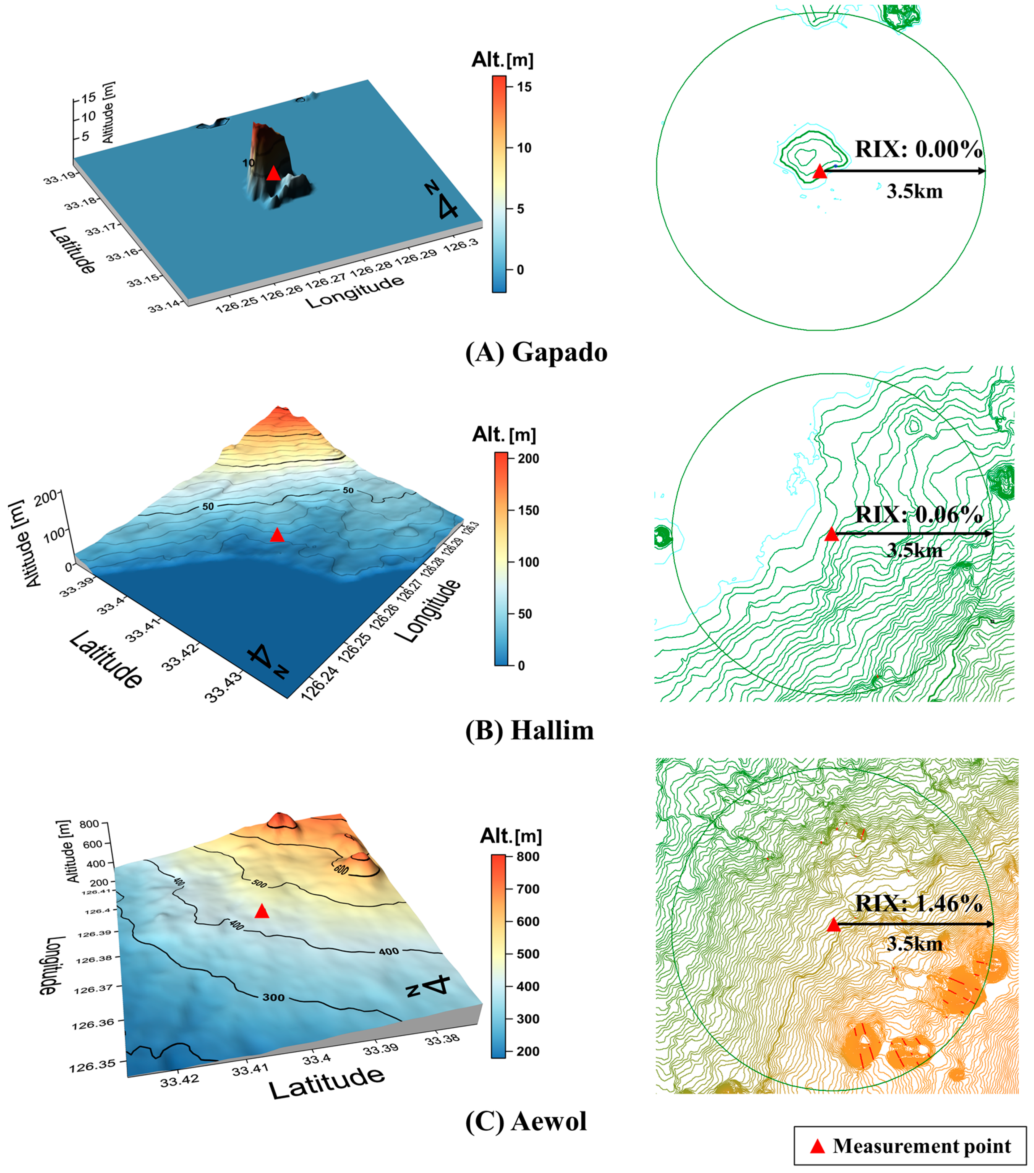
Nine measurement sites containing meteorological observatories were selected for this study, which were divided into three groups in accordance with the topographical conditions: Chujado, Gapado, and Udo for the islet areas; Gujwa, Hallim, and Moseulpo for the coastal areas; and Aewol, Ohdeung, and Sunheul for the inland areas. Figure 2 presents a 3D terrain map and the ruggedness index (RIX) analysis for the sites. Here, Gapado, Hallim, and Aewol were each selected as representative of their respective topographical conditions. Each 3D map has an actual area of about 6 × 6 km and the center of the map coincides with the measurement point. Meanwhile, the RIX indicates the terrain ruggedness or complexity for a given site. The RIX value is defined as the proportion of the surrounding terrain surface which is steeper than a certain critical slope [23,24]. That is, as the RIX value is higher, the complexity of the terrain increases. In this work, a radius of 3.5 km, a critical slope of 0.3, and number of radii of 72 were used for the RIX calculation. The RIX values were 0% at Gapado, 0.06% at Hallim, and 1.46% at Aewol, respectively.
Table 1 shows sites and measurement conditions. The wind speed was measured by wind sensors on the automatic weather system (AWS) at the measurement sites, and also measured at 10–14 m above ground level for five years, from 2009 to 2013. As for the RIX value, the inland area generally rated higher (1.46–4.21%) while the islet (0–0.31%) and coastal areas (0–0.14%) comparatively rated lower.
Before commencing data analysis, data validation was performed to obtain more reliable results. This was done through three measurement data tests which were described by [25,26]: the range test, relation test, and trend test. Wind data showing significant errors on these tests were removed, which turned out to be less than one percent of all measurement data tested. In addition, since the cup anemometer sensor has comparatively high wind speed thresholds, wind speed distribution estimated by cup anemometer wind speed data can cause the exaggeration of the probability of calm or low wind speed [27,28,29]. Accordingly, wind speed data below 0.5 m/s were removed from the measurements. Time and frequency of the removed wind speed data (0–0.5 m/s) are also listed in the Table 1. Ohdeung had the highest value of all the measurement sites at 876.7 h/year (10.0%), while the lowest value of 93.3 h/year (1.1%) appeared at the Udo site. After performing data validation, the data recovery rate was more than 89.8%.
Table 2 shows the specifications for the AWS anemometer. This sensor is the three-cup anemometer, widely used for measuring wind speeds at observatories. Wind speed data were collected at a sampling rate of 4 Hz and averaged over 10-min intervals.
3. Methods for Estimating Weibull Parameters
The Weibull distribution function is commonly used to represent wind speed distribution. It can be described by the probability density function (PDF) and the cumulative distribution function (CDF). The PDF, f(v), and the CDF, F(v), are expressed thus [30,31]
where v is the wind speed, c is the scale parameter with the same wind speed unit (m/s), and k is a unitless shape parameter. The scale parameter determines the abscissa scale on a plot of the distribution, while the shape parameter determines the shape of the distribution.
The wind speed data were analyzed using the six methods for estimating Weibull parameters, which are briefly explained below.
3.1. Empirical Method
3.2. Moment Method
Using Equation (1), the average wind speed and the standard deviation of the wind speed data can be calculated in the equations [7,33,34,35]:
Dividing the square of Equation (5) by the square of Equations (6) and (7) can be obtained.
In Equation (7), the shape parameter, k, can be calculated by the numerical iteration method and the scale parameter, c, can be obtained from Equation (4).
3.3. Graphical Method
The graphical method is calculated using a linear least-squares regression. From a double logarithmic transformation in Equation (2), a new linear regression equation is derived as [15,36]:
Here, a straight line can be drawn through on the x-axis and on the y-axis. The shape parameter, k, is the slope of the straight line and the scale parameter, c, is obtained by the y-intercept of the straight line.
3.4. Energy Pattern Factor Method
This method uses the energy pattern factor, Epf, which is defined [16,37]:
where is the average of wind speed cubed and is the cube of the average wind speed. The shape parameter, k, can be estimated in the equation:
The scale parameter is estimated using Equation (4).
3.5. Maximum Likelihood Method (MLM)
The maximum likelihood method uses time-series wind data for calculating Weibull parameters. Weibull parameters are estimated using the equations [17,37]:
where vi is the wind speed in timestep i and n is the number of nonzero wind speed data points. Equation (11) should be calculated using numerical iteration, and then Equation (12) can be solved.
3.6. Modified Maximum Likelihood Method (MMLM)
This method uses the wind speed frequency which is applied to the MLM. Weibull parameters are calculated as [18,37]:
where vi is the central value of wind speed in bin i, and n is the number of bins. f(vi) is the frequency that the wind speed falls within bin i, and f(v ≥ 0) is the probability that the wind speed equals or exceeds zero.
4. Assessment of Method Accuracy
In order to assess the accuracy of these methods, four accuracy tests were used, which consisted of three error tests (RMSE, the maximum error, and the wind power density (WPD) error) and an analysis of variance, R2. They are described below.
4.1. RMSE
RMSE was used in evaluating the performance of each method statistically. The PDF values obtained from the time-series wind data should be compared with the PDF values obtained by using each method. The RMSE is defined [5,18,38]:
where is the observed PDF value at bin i, and is the estimated PDF value computed by each method at the same bin. n is the number of bins.
4.2. Maximum Error
The maximum error, M, is used to calculate the error of CDF and computed in the equation [18]
where is the observed CDF value at bin, i, and is the estimated CDF value computed by each method at the same bin.
4.3. Wind Power Density (WPD) Error
An important factor in evaluating the economic feasibility of a potential wind farm, the WPD can be given in two types as follows [7,18,39]:
- The average WPD of the Weibull distribution obtained using each method:where ρ is the air density.
- The average WPD of the observed wind speeds:
It is assumed that the air density is constant at 1.225 kg/m3. The WPD error is expressed as a percent error between the results of Equations (17) and (18).
4.4. Analysis of Variance (R2)
The coefficient of determination, R2, indicates how much variance occurs between observed and estimated values, which can be derived using a linear regression analysis method. It can provide a measure of discrepancy between them. It was applied to the Weibull PDF, which is defined by the equation [37]:
where is the observed average PDF value.
5. Consideration of Bin Interval
Before applying the graphical and MMLM methods to the observed wind data, the frequency distribution and the cumulative frequency distribution should be calculated. Before doing so, the bin interval used in these distributions must be determined. Since the bin interval generally has an effect on estimating the Weibull parameters, an appropriate interval should be selected. In this work, because the wind speed data have one decimal place, those were analyzed using 10 bin intervals of 0.1 m/s to 1.0 m/s. Table 3 shows the representative data set with different bin intervals of 0.1, 0.5, and 1.0 m/s at Gapado. It also gives the frequency and the cumulative frequency of the wind data observed.
5.1. Graphical Method
The F(v) of Equation (8) is such that the cumulative frequency distribution as seen in Table 3 and the Weibull parameters could be calculated using a linear least-squares regression method. Then four accuracy tests were applied to the Weibull parameters calculated based on the 10 types of bin intervals. Figure 3 shows the accuracy test results according to bin interval. In order to assess the performance for each bin interval, the average and five-number summary (maximum, minimum, median, first quartile, and third quartile) values were calculated from the accuracy results at all sites. Performance varied considerably with bin interval. Overall, except WPD error, the remaining accuracy tests showed better performance with decreases in bin interval. As for the WPD error, the Weibull parameters were estimated very well for the wind data with bin intervals of 0.6, 0.7, and 0.8 m/s.
5.2. MMLM Method
The f(v) in Equations (13) and (14) is frequency distribution such as that of Table 3, and the Weibull parameters can be calculated using numerical iterations method. The results of the accuracy tests are shown in Figure 4. Unlike the graphical method, all the accuracy tests had similar performance for accurate Weibull parameters regardless of the bin interval. In other words, the performance of the MMLM was not really affected by the bin interval.
Based on the results of the accuracy tests, an appropriate bin interval for each site at the graphical and MMLM methods was presented in Table 4.
6. Results and Discussion
6.1. Comparison of the Methods
Table 5 shows the characteristics of wind speed data for five years at the nine measurement sites. ‘S.D.’ and ‘C.V.’ stand for the standard deviation and the coefficient of variation, respectively. The islet area generally had the highest average wind speed, the widest wind speed range and the lowest C.V. value of all areas. This area was followed by the coastal and inland areas. This might be because the islet areas have fewer obstacles to disturb the wind flow compared to the other areas, as mentioned in [41,42].
To compare the accuracy of the different methods, Weibull parameters c and k were calculated using each method with the observed wind speed data. Then two types of Weibull distributions were obtained by the estimated values of Weibull parameters using Equations (1) and (2). Finally, four accuracy tests were implemented by comparing estimated Weibull distributions with observed wind speed distribution.
Figure 5 shows comparisons of observed wind speed distributions with estimated Weibull PDFs obtained using the six methods for all measurement sites. As shown in the figures, islet areas generally had a wider range in high wind speed than the other areas, followed by coastal and inland areas, possibly owing to differences in terrain. In addition, the graphical method was shown to be the worst among the six methods when compared with the observed wind speed distribution at all sites.
Table 6 shows the estimated Weibull parameters and the accuracy test results using the six methods. The rankings of the methods which were rated using the average values in each test are also presented in Table 6. Two Weibull parameters had various values depending on the method and the site. The islet area generally had the highest values of scale parameter, c, among all the areas, followed by the coastal and inland areas. The islet area has a distribution which is wider in high wind speed range than the other areas, resulting in the comparatively high values of Weibull scale parameter. As for shape parameter, k, overall, there was a tendency that higher k was found in islet areas and lower k appeared in inland area.
As for the RMSE and maximum error, Chujado and Udo showed the best performance while Ohdeung and Aewol had the worst performance. It was confirmed that most of the errors came out of the low speed range as shown in Figure 5 such that the accuracy of the methods was determined according to how well the methods fit the low speed range of the observed data. In the WPD error, Gujwa showed the best performance while Ohdeung showed the worst. Generally, the sites with values close to zero in both skew and kurtosis showed better results after factoring in WPD error. In fact, Gapado, Udo, and Gujwa (skew: 0.6–0.8, kurtosis: 0.5) showed better performance than did the other sites. The former yielded positive lower values in both skew and kurtosis as shown in Table 5, while Ohdeung showed the worst, yielding the highest values among the sites (skew: 1.8 and kurtosis: 6.6). In the analysis of variance (R2), Chujado had the best performance while Aewol showed the worst.
Based on Table 6, performance results are plotted according to the method in Figure 6, which shows the average and five-number summary (maximum, minimum, median, first quartile, and the third quartile) values calculated from the accuracy results for all sites. In conclusion, on the whole, it was found that the best method for estimating Weibull parameters was the moment method. The moment method showed the best performance among the two tests: the RMSE, the analysis of variance, R2. Furthermore, it showed the second-best performance in terms of the WPD error and the fourth-best performance in terms of maximum error. Next, the energy pattern factor method had the second-best accuracy in all the accuracy tests, followed by the empirical method. In particular, the energy pattern factor method showed the best result in terms of the WPD error for all sites. Since the equation for this method uses the energy pattern factor, Epf, which is calculated from the average of wind speed cubed, , the estimated Weibull parameters from this method generally apply to the distribution of wind speed cubed and also decrease the WPD error.
On the other hand, the graphical method showed the worst performance of the six methods. As pointed out by Seguro and Lambert [17], the graphical method uses cumulative wind speed frequency distribution, not real wind speed data, to find the linear least-squares regression line, which leads to each bin weighted equally regardless of the number of data. That is the main reason why the graphical method is somewhat inaccurate compared to other methods. Meanwhile, in this work, the MLM and MMLM methods resulted in the second and third worst performances. In comparison with other studies [17,18,19,21], the MLM and MMLM methods showed better performances for estimating Weibull parameters, which was against the result of this work. Since wind speed data less than 0.5 m/s were not used to estimate Weibull parameters in this work, that seems to have affected the performance of the estimation. Furthermore, because the MLM and MMLM methods use the logarithmic equations to estimate the shape parameter, k, values lower than 0.5 m/s might affect the computation of these logarithmic equations.
6.2. Impact of Topographical Conditions on the Performance of the Methods
The results of the accuracy tests according to the topographical conditions are indicated in Table 7. Although accuracy ranking of the methods is not consistent depending on the accuracy tests, it is similar for each accuracy test regardless of the topographical conditions. In other words, there were no better methods relying on specific terrain conditions for estimating Weibull parameters more accurately.
On the other hand, the error values themselves such as RMSE, maximum error, and WPD error were dependent on the variation of topographical conditions. That is, the islet area showed the least error values in almost all methods for estimating Weibull parameters, followed by the coastal and inland areas. Similar tendency was found at the R2 test, where the islet area had the biggest R2 value in all the terrain conditions.
In conclusion, when the Weibull distribution is used as a statistical model for wind speed distribution in order to assess economic feasibility of a wind power project, the different estimation uncertainty for Weibull parameters should be applied based on the topographical condition. That is, as terrain complexity increases, the higher uncertainty should be used for estimating Weibull parameters. Actually, the WPD error by the moment method showed the difference of 0.486–5.017% with variation of the topographical conditions in Table 7.
6.3. Wind Resource Extrapolation
The Weibull distributions have been used to assess potential wind energy. The accurate assessment for wind energy at wind farm sites is important for reliable economic evaluation. The average wind speed and the wind power density have been used as simple but important factors for evaluating wind energy resources at a given site. Those should be estimated based on a hub height of a wind turbine.
In this investigation, the average wind speed and wind power density were estimated for all sites studied. A hub height was assumed to be 100 m because wind turbines with more than 100 m hub height are currently common. However, the wind speed was actually measured at 10–14 m height and therefore the wind speed should be extrapolated to a target height of 100 m. There are some mathematical models to estimate the wind speed at a required height. Of them, the power law is the most common method and can be expressed as [25,30,31]:
where v1 and v2 are simultaneous wind speeds at heights of h1 and h2 respectively and exponent α is power law exponent.
In order to calculate the power law exponent, at least two wind speed measurements at different heights are required but the measurements at a single height were only used in this study. Thus, Equation (20) could not be directly applied for extrapolation in this study. However, another way of handling power law method was suggested by Justus and Mikhail [33]. They estimated power law exponent using Weibull distribution and power law exponent can be expressed as the equation [30,33,43]:
where is Weibull scale parameter known at a height of h1.
In addition, the relevant formula with Weibull parameters was also suggested in the two equations [33,43]:
where , and , are Weibull scale and shape parameters at heights of h1 and h2, respectively. Average wind speed at a target height (e.g., a hub height of the wind turbine) can be estimated using Equation (5) where two Weibull parameters, c and k, at a target height were calculated using Equations (21)–(23) with known values of Weibull parameters at a different height. Meanwhile, wind power density at a target height can be estimated using Equation (17) with those parameters calculated.
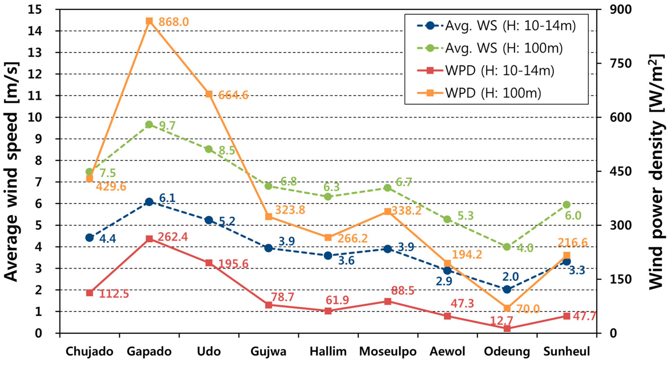
Figure 7 shows five-year average wind speeds and wind power densities for all measurement sites. In addition to the average wind speed and the wind power density at a hub height of 100 m, those at measurement heights of 10–14 m were also provided in the Figure. Here, the air density is assumed to be constant at 1.225 kg/m3. Additionally, the average wind speed and the wind power density at 10–14 m height were calculated from actual wind speed data but wind speed less than 0.5 m/s was not used for the calculation. The estimated 10–14 m-high Weibull parameters were required to estimate Weibull parameters at 100 m height. Thus the 10–14 m-high Weibull parameters were brought from the values estimated by the moment method in Table 6, because the moment method was assessed as the most accurate method in this study.
In Figure 7, the islet area had the highest average wind speed and wind power density among the three types of terrain conditions, followed by the coastal and inland areas. The average wind speed and the wind power density in Gapado were higher than those in the other sites and were 9.7 m/s and 868.0 W/m2 at 100 m height. On the other hand, Odeung was the lowest in all the sites which were 4.0 m/s and 70.0 W/m2 at 100 m height. It should be noted that estimated average wind speed and the wind power density might be exaggerated since that those were estimated under the condition that wind speed measurements less than 0.5 m/s were not used for the estimation.
7. Conclusions
The six methods for estimating Weibull parameters were introduced and their accuracy was evaluated using four accuracy tests applied to each. Five-year wind data taken from nine Jeju sites consisting of three different topographical conditions were analyzed to raise the reliability for evaluation purposes. Additionally, the effect of variation in topographical conditions on the accuracy of the estimation methods was evaluated. In addition, 10 bin interval types were considered for graphical and MMLM methods to assess how much the bin interval affected the performances of these methods. The results are summarized as follows:
- (1)
- When applying the MMLM, the bin interval did not significantly affect the performance of the estimation whereas for the graphical method, the performance depended on the bin interval. The graphical method suggested a better performance as bin interval decreased in the accuracy tests of RMSE, maximum error, and R2.
- (2)
- The variation in topographical conditions did not affect the accuracy ranking of the methods and there were no better methods relying on specific terrain condition.
- (3)
- As terrain complexity increased, the estimation uncertainty for Weibull parameters also increased. Therefore, in order to evaluate the economic feasibility, future wind farm developers should take into account different estimation uncertainties for the Weibull distribution based on the variation in topographical conditions.
- (4)
- The moment method performed the best and was the most accurate for all topographical conditions among the six methods. The energy pattern factor and empirical methods were ranked next best.
- (5)
- The graphical method performed the worst among the six methods in this study.
- (6)
- The observed distribution containing values close to zero in both skewness and kurtosis shows the best performance of the WPD error.
For future work, it is necessary to employ new statistical models for fitting wind speed distribution including a typical day model [44], which can extract the samples based on the matrix with suitable dimensions.
Acknowledgments
The work was supported with funding provided by the Korea Institute of Energy Technology Evaluation and Planning (KETEP) and the Ministry of Trade, Industry & Energy (MOTIE) of Republic of Korea (no. 20163010024560), and “Human Resources Program in Energy Technology” of them (no. 20164030201230).
Author Contributions
A major part of the work was done by Dongbum Kang. He analyzed the data and wrote a manuscript. Kyungnam Ko contributed the format of a paper and thoroughly reviewed the manuscript. Jongchul Huh provided the necessary data for the analysis and coordinated the main theme.
Conflicts of Interest
The authors declare no conflict of interest.
Nomenclature
| c | Scale parameter of Weibull distribution (m/s) |
| Epf | Energy pattern factor, dimensionless |
| f(v) | Probability density function |
| F(v) | Cumulative distribution function |
| h | Height (m) |
| k | Shape parameter of Weibull distribution, dimensionless |
| n | Number of observations performed |
| v | Wind speed (m/s) |
| Average wind speed (m/s) | |
| Average of wind speed cubed (m3/s3) | |
| vi | Observed wind speed in stage, i, (m/s) |
| Greek Letters | |
| α | Power law exponent, dimensionless |
| ρ | Air density (kg/m3) |
| σ | Standard deviation of wind speed (m/s) |
Abbreviation
| AWS | Automatic weather system |
| CDF | Cumulative distribution function |
| C.V. | Coefficient of variation |
| MLM | Maximum likelihood method |
| MMLM | Modified maximum likelihood method |
| Probability density function | |
| RIX | Ruggedness index |
| RMSE | Root mean square error |
| S.D. | Standard deviation |
| WPD | Wind power density |
References
- Global Wind Energy Council (GWEC). Global Wind Report 2016; GWEC: Brussels, Belgium, 2017; pp. 12–19. [Google Scholar]
- Korea Wind Energy Industry Association (KWEIA). Korean Wind Energy Statistics Report. Available online: http://www.kweia.or.kr/ (accessed on 20 December 2017).
- Azad, A.K.; Rasul, M.G.; Yusaf, T. Statistical diagnosis of the best weibull methods for wind power assessment for agricultural applications. Energies 2014, 7, 3056–3085. [Google Scholar] [CrossRef]
- Akpinar, E.K.; Akpinar, S. Determination of the wind energy potential for Maden-Elazig, Turkey. Energy Convers. Manag. 2004, 45, 2901–2914. [Google Scholar] [CrossRef]
- Arslan, T.; Bulut, Y.M.; Altın Yavuz, A. Comparative study of numerical methods for determining Weibull parameters for wind energy potential. Renew. Sustain. Energy Rev. 2014, 40, 820–825. [Google Scholar] [CrossRef]
- Ali, S.; Lee, S.; Jang, C. Techno-economic assessment of wind energy potential at three locations in South Korea using long-term measured wind data. Energies 2017, 10, 1442. [Google Scholar] [CrossRef]
- Shu, Z.R.; Li, Q.S.; Chan, P.W. Investigation of offshore wind energy potential in Hong Kong based on Weibull distribution function. Appl. Energy 2015, 156, 362–373. [Google Scholar] [CrossRef]
- Kadhem, A.A.; Wahab, I.N.; Aris, I.; Jasni, J.; Abdalla, N.A. Advanced wind Speed prediction model based on a combination of Weibull distribution and an artificial neural network. Energies 2017, 10, 1744. [Google Scholar] [CrossRef]
- Herrero-Novoa, C.; Pérez, I.A.; Sánchez, M.L.; García, M.Á.; Pardo, N.; Fernández-Duque, B. Wind speed description and power density in northern Spain. Energy 2017, 138, 967–976. [Google Scholar] [CrossRef]
- Akdağ, S.A.; Bagiorgas, H.S.; Mihalakakou, G. Use of two-component Weibull mixtures in the analysis of wind speed in the Eastern Mediterranean. Appl. Energy 2010, 87, 2566–2573. [Google Scholar] [CrossRef]
- Carta, J.A.; Ramírez, P. Analysis of two-component mixture Weibull statistics for estimation of wind speed distributions. Renew. Energy 2007, 32, 518–531. [Google Scholar] [CrossRef]
- Gómez-Lázaro, E.; Bueso, M.; Kessler, M.; Martin-Martinez, S.; Zhang, J.; Hodge, B.; Molina-Garcia, A. Probability Density Function Characterization for Aggregated Large-Scale Wind Power Based on Weibull Mixtures. Energies 2016, 9, 91. [Google Scholar] [CrossRef]
- Justus, C.G.; Hargraves, W.R.; Mikhail, A.; Graber, D. Methods for estimating wind speed frequency distributions. J. Appl. Meteorol. 1978, 17, 350–353. [Google Scholar] [CrossRef]
- Stevens, M.J.M.; Smulders, P.T. Estimation of the parameters of the Weibull wind speed distribution for wind energy utilization purposes. Wind Eng. 1979, 3, 132–145. [Google Scholar]
- Deaves, D.M.; Lines, I.G. On the fitting of low mean wind speed data to the Weibull distribution. J. Wind Eng. Ind. Aerodyn. 1997, 66, 169–178. [Google Scholar] [CrossRef]
- Akdag, S.A.; Dinler, A. A new method to estimate Weibull parameters for wind energy applications. Energy Convers. Manag. 2009, 50, 1761–1766. [Google Scholar] [CrossRef]
- Seguro, J.V.; Lambert, T.W. Modern estimation of the parameters of the Weibull wind speed distribution for wind energy analysis. J. Wind Eng. Ind. Aerodyn. 2000, 85, 75–84. [Google Scholar] [CrossRef]
- Chang, T.P. Performance comparison of six numerical methods in estimating Weibull parameters for wind energy application. Appl. Energy 2011, 88, 272–282. [Google Scholar] [CrossRef]
- Saleh, H.; Abou El-Azm Aly, A.; Abdel-Hady, S. Assessment of different methods used to estimate Weibull distribution parameters for wind speed in Zafarana wind farm, Suez Gulf, Egypt. Energy 2012, 44, 710–719. [Google Scholar] [CrossRef]
- Mohammadi, K.; Alavi, O.; Mostafaeipour, A.; Goudarzi, N.; Jalilvand, M. Assessing different parameters estimation methods of Weibull distribution to compute wind power density. Energy Convers. Manag. 2016, 108, 322–335. [Google Scholar] [CrossRef]
- Alavi, O.; Sedaghat, A.; Mostafaeipour, A. Sensitivity analysis of different wind speed distribution models with actual and truncated wind data: A case study for Kerman, Iran. Energy Convers. Manag. 2016, 120, 51–61. [Google Scholar] [CrossRef]
- Jeju Special Self-Governing Province. Administrative Statistics Information. Available online: http://www.jeju.go.kr/ (accessed on 20 December 2017).
- Bowen, A.J.; Mortensen, N.G. WAsP Prediction Errors Due to Site Orography; Risø National Laboratory: Roskilde, Denmark, 2004; ISBN 87-550-2320-7. [Google Scholar]
- Taylor, P.A.; Walmsley, J.L.; Salmon, J.R. A simple model of neutrally stratified boundary-layer flow over real terrain incorporating wavenumber-dependent scaling. Bound-Layer Meteorol. 1983, 26, 169–189. [Google Scholar] [CrossRef]
- Brower, M.C. Wind Resource Assessment; John Wiley & Sons, Inc.: Hoboken, NJ, USA, 2012; pp. 117–144. ISBN 978-1118022320. [Google Scholar]
- Measnet. Evaluation of Site-Specific Wind Conditions, version 1; Measnet: Madrid, Spain, 2009; pp. 14–18. [Google Scholar]
- Takle, E.S.; Brown, J.M. Note on the use of Weibull Statistics to characterize wind-speed data. J. Appl. Meteorol. Climatol. 1978, 17, 556–559. [Google Scholar] [CrossRef]
- Carrillo, C.; Cidrás, J.; Díaz-Dorado, E.; Obando-Montaño, A.F. An Approach to determine the Weibull parameters for wind energy analysis: The case of Galicia (Spain). Energies 2014, 7, 2676–2700. [Google Scholar] [CrossRef]
- Carta, J.A.; Ramírez, P.; Velázquez, S. A review of wind speed probability distributions used in wind energy analysis: Case studies in the Canary Islands. Renew. Sustain. Energy Rev. 2009, 13, 933–955. [Google Scholar] [CrossRef]
- Manwell, J.F.; McGowan, J.G.; Rogers, A.L. Wind Energy Explained: Theory, Design and Application, 1st ed.; John Wiley & Sons, Inc.: Chichester, UK, 2002; pp. 46–62. ISBN 978-0-470-01500-1. [Google Scholar]
- Jain, P. Wind Energy Engineering; McGraw-Hill Companies, Inc.: New York, NY, USA, 2011; pp. 26–37. ISBN 978-0071714778. [Google Scholar]
- Basumatary, H.; Sreevalsan, E.; Sasi, K.K. Weibull parameter estimation—A comparison of different methods. Wind Eng. 2005, 29, 309–316. [Google Scholar] [CrossRef]
- Justus, C.G.; Mikhail, A. Height variation of wind speed and wind distributions statistics. Geophys. Res. Lett. 1976, 3, 261–264. [Google Scholar] [CrossRef]
- Dorvlo, A.S.S. Estimating wind speed distribution. Energy Convers. Manag. 2002, 43, 2311–2318. [Google Scholar] [CrossRef]
- Gebizlioglu, O.L.; Şenoğlu, B.; Kantar, Y.M. Comparison of certain value-at-risk estimation methods for the two-parameter Weibull loss distribution. J. Comput. Appl. Math. 2011, 235, 3304–3314. [Google Scholar] [CrossRef]
- Lun, I.Y.F.; Lam, J.C. A study of Weibull parameters using long-term wind observations. Renew. Energy 2000, 20, 145–153. [Google Scholar] [CrossRef]
- Costa Rocha, P.A.; de Sousa, R.C.; de Andrade, C.F.; da Silva, M.E.V. Comparison of seven numerical methods for determining Weibull parameters for wind energy generation in the northeast region of Brazil. Appl. Energy 2012, 89, 395–400. [Google Scholar] [CrossRef]
- De Andrade, C.F.; Maia Neto, H.F.; Costa Rocha, P.A.; Vieira da Silva, M.E. An efficiency comparison of numerical methods for determining Weibull parameters for wind energy applications: A new approach applied to the northeast region of Brazil. Energy Convers. Manag. 2014, 86, 801–808. [Google Scholar] [CrossRef]
- Dahbi, M.; Benatiallah, A.; Sellam, M. The Analysis of Wind Power Potential in Sahara Site of Algeria-an Estimation Using the ‘Weibull’ Density Function. Energy Procedia 2013, 36, 179–188. [Google Scholar] [CrossRef]
- Garcia, A.; Torres, J.L.; Prieto, E.; de Francisco, A. Fitting wind speed distributions: A case study. Sol. Energy 1998, 62, 139–144. [Google Scholar] [CrossRef]
- Ko, K.; Kim, K.; Huh, J. Characteristics of wind variations on Jeju Island, Korea. Int. J. Energy Res. 2010, 34, 36–45. [Google Scholar] [CrossRef]
- Ko, K.; Kim, K.; Huh, J. Variations of wind speed in time on Jeju Island, Korea. Energy 2010, 35, 3381–3387. [Google Scholar] [CrossRef]
- Gualtieri, G.; Secci, S. Methods to extrapolate wind resource to the turbine hub height based on power law: A 1-h wind speed vs. Weibull distribution extrapolation comparison. Renew. Energy 2012, 43, 183–200. [Google Scholar] [CrossRef]
- Fortuna, L.; Nunnari, G.; Nunnari, S. A new fine-grained classification strategy for solar daily radiation patterns. Pattern Recognit. Lett. 2016, 81, 110–117. [Google Scholar] [CrossRef]
Figure 1.
Location of Jeju Island and its measurement sites.

Figure 2.
3D images and RIX analysis for the measurement sites.

Figure 3.
The results of the accuracy tests according to bin interval (graphical method). (a) RMSE; (b) Maximum error; (c) WPD error; (d) R2.
Figure 3.
The results of the accuracy tests according to bin interval (graphical method). (a) RMSE; (b) Maximum error; (c) WPD error; (d) R2.

Figure 4.
The results of the accuracy tests according to bin interval (MMLM). (a) RMSE; (b) Maximum error; (c) WPD error; (d) R2.
Figure 4.
The results of the accuracy tests according to bin interval (MMLM). (a) RMSE; (b) Maximum error; (c) WPD error; (d) R2.
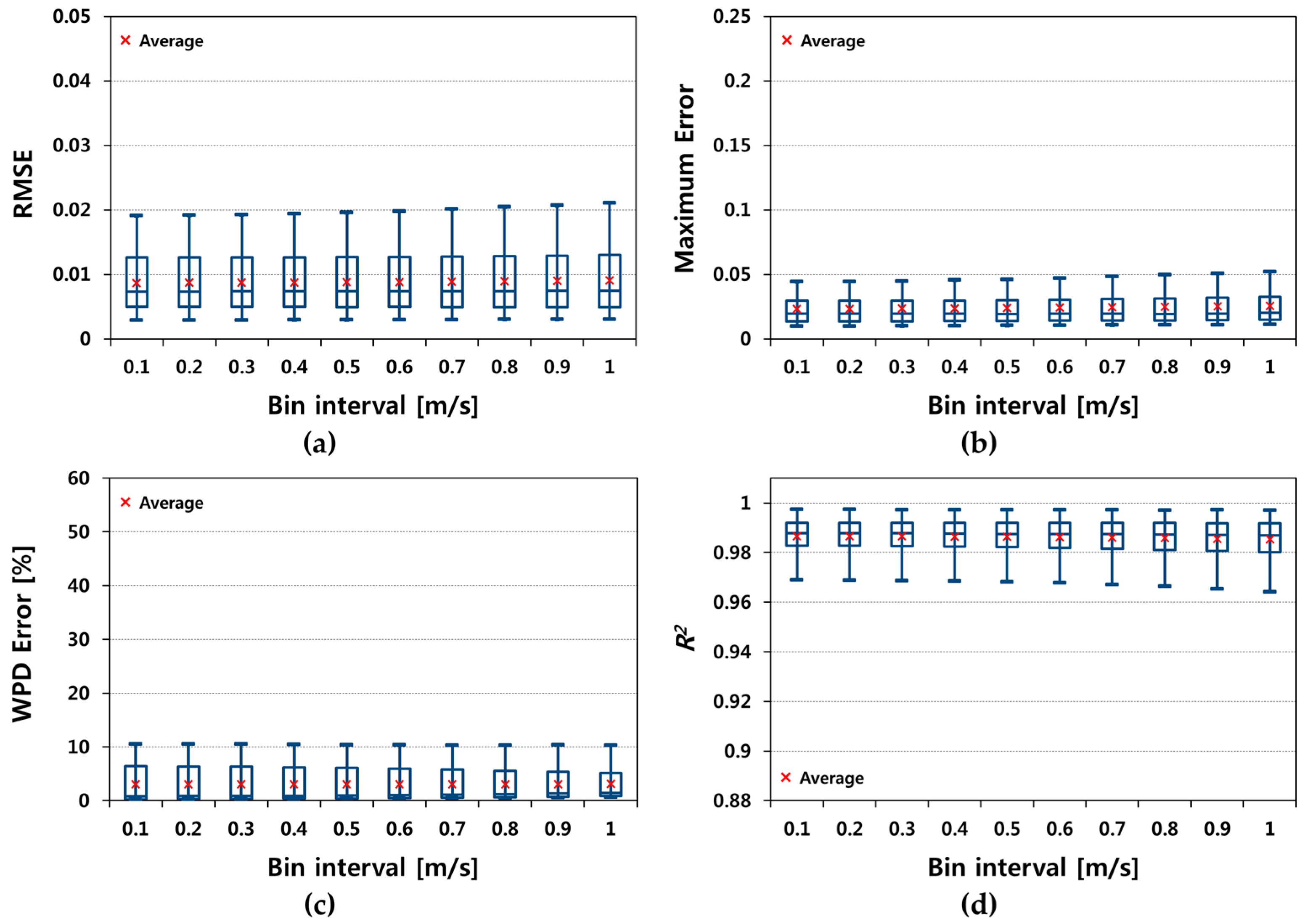
Figure 5.
A comparison between the observed wind speed distributions and estimated Weibull PDFs.
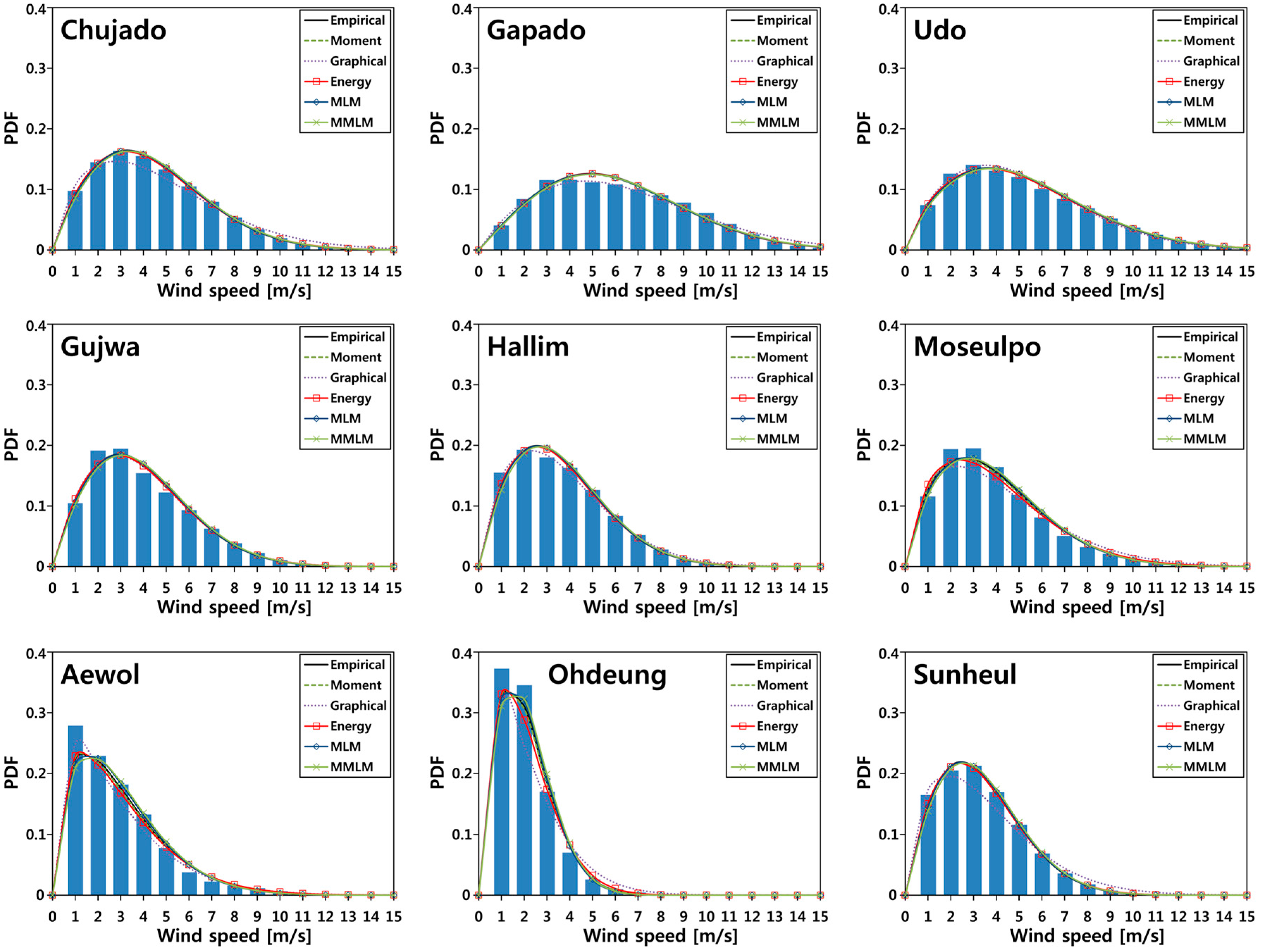
Figure 6.
The accuracy test performance of each method. (a) RMSE; (b) Maximum error; (c) WPD error; (d) R2.
Figure 6.
The accuracy test performance of each method. (a) RMSE; (b) Maximum error; (c) WPD error; (d) R2.
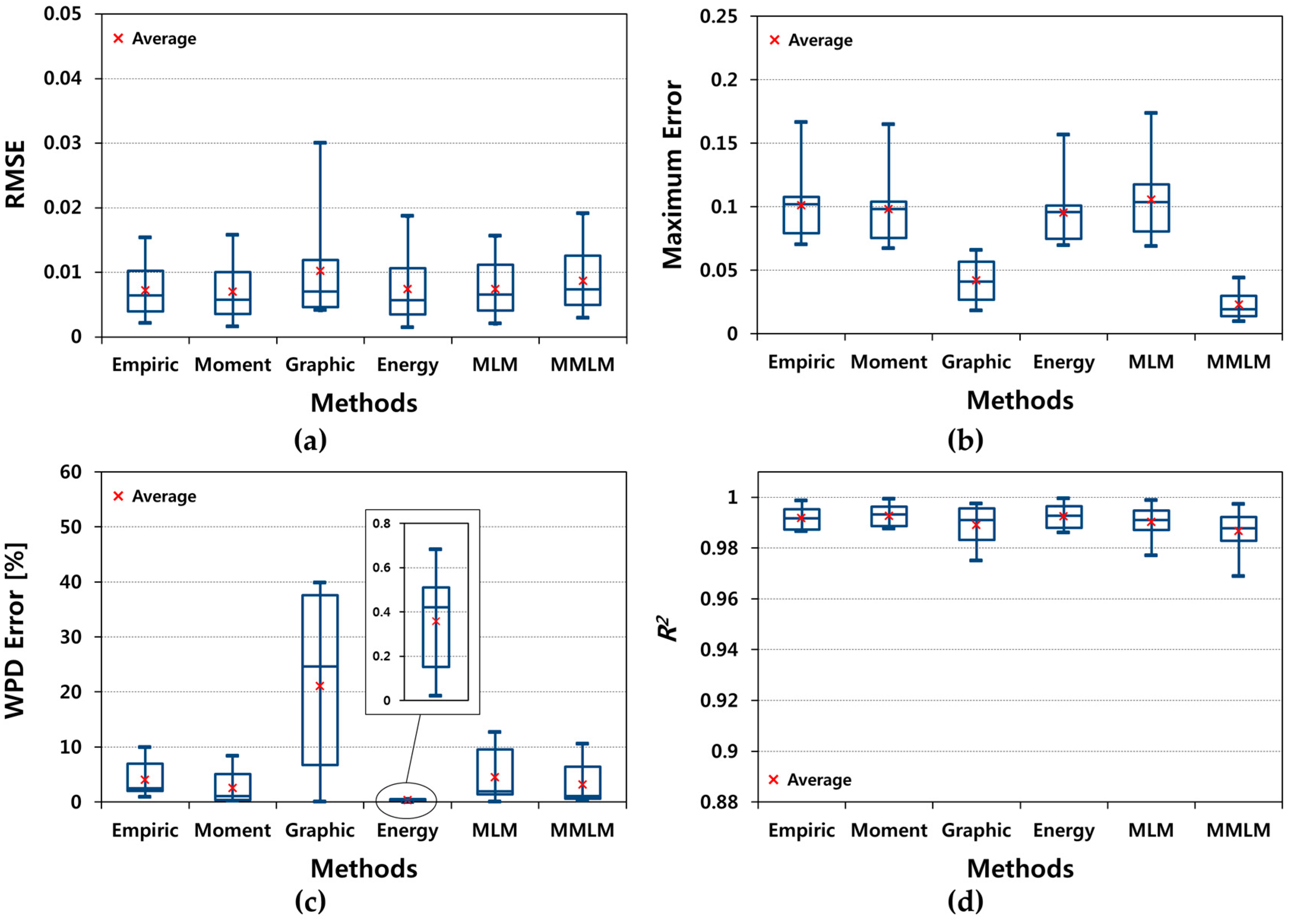
Figure 7.
Five-year average wind speed and wind power density for all measurement sites.


Table 1.
Sites and measurement conditions. Freq.: Frequency.
| Sites | Position | Altitude (m) | Data Recovery Rate (%) | Time of 0–0.5 m/s (h/Year) (Freq.) | RIX (%) | Topographical Condition |
|---|---|---|---|---|---|---|
| Chujado | 126°18′02″ E | 18 | 95.0 | 404.8 (4.6%) | 0.00 | Islet |
| 33°57′16″ N | ||||||
| Gapado | 126°16′24″ E | 13 | 97.6 | 165.3 (1.9%) | 0.00 | |
| 33°09′58″ N | ||||||
| Udo | 126°57′12″ E | 39 | 98.6 | 93.3 (1.1%) | 0.31 | |
| 33°30′23″ N | ||||||
| Gujwa | 126°51′06″ E | 25 | 98.2 | 137.6 (1.6%) | 0.00 | Coastal |
| 33°31′21″ N | ||||||
| Hallim | 126°16′02″ E | 22 | 94.7 | 439.8 (5.0%) | 0.06 | |
| 33°24′37″ N | ||||||
| Moseulpo | 126°14′60″ E | 12 | 96.8 | 259.8 (3.0%) | 0.14 | |
| 33°13′00″ N | ||||||
| Aewol | 126°22′48″ E | 447 | 93.9 | 502.9 (5.8%) | 1.46 | Inland |
| 33°23′60″ N | ||||||
| Ohdeung | 126°32′38″ E | 513 | 89.8 | 876.7 (10.0%) | 3.53 | |
| 33°25′25″ N | ||||||
| Sunheul | 126°42′42″ E | 341 | 93.1 | 575.7 (6.6%) | 4.21 | |
| 33°27′30″ N |
Table 2.
Anemometer specifications.
| Items | Specification |
|---|---|
| Model | WM-4-WS |
| Measuring range | 0–70 m/s |
| Sampling rate | 4 Hz |
| Threshold | Below 0.3 m/s |
| Resolution | 0.1 m/s |
| Accuracy | 0–10 m/s: <0.3 m/s Over 10 m/s: <3% |
| Operation temperature | −40–+80 °C |
| Type | 3-cup anemometer |
Table 3.
The sample data set (site: Gapado). Cum.: Cumulative; Freq.: Frequency.
| Bin Interval (1 m/s) | Bin Interval (0.5 m/s) | Bin Interval (0.1 m/s) | ||||||
|---|---|---|---|---|---|---|---|---|
| Bin (m/s) | Freq. (%) | Cum. Freq. (%) | Bin (m/s) | Freq. (%) | Cum. Freq. (%) | Bin (m/s) | Freq. (%) | Cum. Freq. (%) |
| 0.5–1.5 | 4.03 | 4.03 | 0.5–1.0 | 1.65 | 1.65 | 0.5–0.6 | 0.29 | 0.29 |
| 1.5–2.5 | 8.38 | 12.41 | 1.0–1.5 | 2.38 | 4.03 | 0.6–0.7 | 0.29 | 0.58 |
| 2.5–3.5 | 11.51 | 23.92 | 1.5–2.0 | 3.58 | 7.60 | 0.7–0.8 | 0.33 | 0.91 |
| 3.5–4.5 | 11.56 | 35.48 | 2.0–2.5 | 4.80 | 12.41 | 0.8–0.9 | 0.34 | 1.25 |
| 4.5–5.5 | 11.15 | 46.62 | 2.5–3.0 | 5.68 | 18.08 | 0.9–1.0 | 0.40 | 1.65 |
| 5.5–6.5 | 10.80 | 57.43 | 3.0–3.5 | 5.83 | 23.92 | 1.0–1.1 | 0.39 | 2.03 |
| 6.5–7.5 | 9.97 | 67.40 | 3.5–4.0 | 5.87 | 29.79 | 1.1–1.2 | 0.45 | 2.48 |
| 7.5–8.5 | 9.02 | 76.42 | 4.0–4.5 | 5.69 | 35.48 | 1.2–1.3 | 0.47 | 2.95 |
| 8.5–9.5 | 7.79 | 84.21 | 4.5–5.0 | 5.63 | 41.10 | 1.3–1.4 | 0.51 | 3.46 |
| 9.5–10.5 | 6.07 | 90.28 | 5.0–5.5 | 5.52 | 46.62 | 1.4–1.5 | 0.56 | 4.03 |
| ≥10.5 | 9.72 | 100 | ≥5.5 | 53.38 | 100 | ≥1.5 | 95.97 | 100 |
Table 4.
The appropriate bin intervals for the sites.
| Methods | Bin Interval (m/s) | ||||||||
|---|---|---|---|---|---|---|---|---|---|
| Chujado | Gapado | Udo | Gujwa | Hallim | Moseulpo | Aewol | Odeung | Sunheul | |
| Graphical | 0.1 | 0.1 | 0.4 | 0.3 | 0.2 | 0.3 | 0.5 | 0.2 | 0.1 |
| MMLM | 0.1 | 1 | 1 | 1 | 0.1 | 0.1 | 0.1 | 0.1 | 0.1 |
Table 5.
Wind speed data characteristics for the three area types.
| Sites | No. of Data | Average (m/s) | Mode (m/s) | Speed Range (m/s) | S.D. (m/s) | C.V. (%) | Skew-Ness | Kurtosis | |
|---|---|---|---|---|---|---|---|---|---|
| Islet | Chujado | 249,708 | 4.4 | 3.1 | 28.3 | 2.5 | 56.6 | 0.9 | 1.5 |
| Gapado | 256,521 | 6.1 | 3.4 | 31.0 | 3.2 | 52.2 | 0.6 | 0.5 | |
| Udo | 259,337 | 5.2 | 2.8 | 20.9 | 3.1 | 59.3 | 0.8 | 0.5 | |
| Coastal | Gujwa | 258,246 | 3.9 | 2.6 | 17.2 | 2.2 | 56.3 | 0.8 | 0.5 |
| Hallim | 249,066 | 3.6 | 1.8 | 18.3 | 2.1 | 58.0 | 0.9 | 1.0 | |
| Moseulpo | 254,620 | 3.9 | 2.5 | 23.4 | 2.4 | 61.1 | 1.4 | 3.2 | |
| Inland | Aewol | 246,856 | 2.9 | 0.9 | 19.6 | 2.1 | 71.7 | 1.7 | 4.1 |
| Ohdeung | 236,021 | 2.0 | 1.3 | 14.8 | 1.2 | 60.4 | 1.8 | 6.6 | |
| Sunheul | 244,848 | 3.3 | 2.4 | 25.6 | 1.9 | 56.4 | 0.9 | 1.2 | |
Table 6.
The estimated Weibull parameters and the results of the accuracy tests.
| Parameters | Methods | Islet | Coastal | Inland | Avg. (Rank) | ||||||
|---|---|---|---|---|---|---|---|---|---|---|---|
| Chujado | Gapado | Udo | Gujwa | Hallim | Moseulpo | Aewol | Ohdeung | Sunheul | |||
| k | Empirical | 1.8547 | 2.0253 | 1.7652 | 1.8664 | 1.8085 | 1.7080 | 1.4357 | 1.7276 | 1.8622 | - |
| Moment | 1.8305 | 2.0025 | 1.7407 | 1.8422 | 1.7841 | 1.6836 | 1.4147 | 1.7032 | 1.8380 | - | |
| Graphical | 1.5987 | 1.8421 | 1.7672 | 1.8197 | 1.6688 | 1.5376 | 1.2660 | 1.3523 | 1.5283 | - | |
| Energy | 1.8204 | 2.0186 | 1.7418 | 1.8353 | 1.7808 | 1.6246 | 1.3718 | 1.5933 | 1.8257 | - | |
| MLM | 1.8504 | 2.0110 | 1.7695 | 1.8771 | 1.8111 | 1.7429 | 1.5092 | 1.7825 | 1.8664 | - | |
| MMLM | 1.8756 | 2.0281 | 1.7857 | 1.8984 | 1.8412 | 1.7671 | 1.5376 | 1.8243 | 1.8988 | - | |
| C (m/s) | Empirical | 4.9824 | 6.8656 | 5.8774 | 4.4357 | 4.0436 | 4.3757 | 3.1992 | 2.2749 | 3.7469 | - |
| Moment | 4.9797 | 6.8643 | 5.8727 | 4.4334 | 4.0409 | 4.3714 | 3.1923 | 2.2728 | 3.7450 | - | |
| Graphical | 5.1954 | 7.1691 | 5.6966 | 4.4237 | 4.0590 | 4.5490 | 2.9645 | 2.2676 | 3.8327 | - | |
| Energy | 4.9785 | 6.8652 | 5.8729 | 4.4327 | 4.0405 | 4.3591 | 3.1766 | 2.2606 | 3.7439 | - | |
| MLM | 4.9910 | 6.8704 | 5.8947 | 4.4513 | 4.0545 | 4.4011 | 3.2424 | 2.2921 | 3.7571 | - | |
| MMLM | 5.0510 | 6.9340 | 5.9581 | 4.5160 | 4.1148 | 4.4615 | 3.3059 | 2.3508 | 3.8166 | - | |
| RMSE | Empirical | 0.0021 | 0.0051 | 0.0041 | 0.0075 | 0.0065 | 0.0068 | 0.0130 | 0.0153 | 0.0039 | 0.0071 (2) |
| Moment | 0.0016 | 0.0048 | 0.0036 | 0.0072 | 0.0058 | 0.0072 | 0.0129 | 0.0157 | 0.0034 | 0.0069 (1) | |
| Graphical | 0.0067 | 0.0047 | 0.0040 | 0.0071 | 0.0045 | 0.0122 | 0.0117 | 0.0300 | 0.0103 | 0.0101 (6) | |
| Energy | 0.0014 | 0.0050 | 0.0037 | 0.0072 | 0.0057 | 0.0085 | 0.0128 | 0.0186 | 0.0033 | 0.0074 (3) | |
| MLM | 0.0020 | 0.0049 | 0.0042 | 0.0078 | 0.0066 | 0.0067 | 0.0146 | 0.0156 | 0.0040 | 0.0074 (4) | |
| MMLM | 0.0029 | 0.0050 | 0.0049 | 0.0088 | 0.0078 | 0.0074 | 0.0164 | 0.0190 | 0.0054 | 0.0086 (5) | |
| Maximum error | Empirical | 0.0815 | 0.0702 | 0.0771 | 0.1073 | 0.1030 | 0.0956 | 0.1080 | 0.1663 | 0.1020 | 0.1012 (5) |
| Moment | 0.0780 | 0.0672 | 0.0731 | 0.1042 | 0.0991 | 0.0922 | 0.1041 | 0.1646 | 0.0983 | 0.0979 (4) | |
| Graphical | 0.0411 | 0.0375 | 0.0278 | 0.0259 | 0.0182 | 0.0504 | 0.0658 | 0.0633 | 0.0478 | 0.0420 (2) | |
| Energy | 0.0765 | 0.0693 | 0.0732 | 0.1033 | 0.0986 | 0.0871 | 0.0957 | 0.1565 | 0.0964 | 0.0952 (3) | |
| MLM | 0.0818 | 0.0687 | 0.0789 | 0.1105 | 0.1044 | 0.1028 | 0.1246 | 0.1737 | 0.1038 | 0.1055 (6) | |
| MMLM | 0.0096 | 0.0180 | 0.0193 | 0.0296 | 0.0178 | 0.0303 | 0.0288 | 0.0439 | 0.0096 | 0.0230 (1) | |
| WPD error (%) | Empirical | 2.494 | 0.899 | 1.852 | 2.293 | 2.118 | 6.257 | 7.734 | 9.915 | 2.610 | 4.019 (4) |
| Moment | 1.048 | 0.218 | 0.192 | 0.867 | 0.565 | 4.551 | 5.553 | 8.315 | 1.182 | 2.499 (2) | |
| Graphical | 36.603 | 25.641 | 10.775 | 0.021 | 10.780 | 24.591 | 2.605 | 38.504 | 39.786 | 21.034 (6) | |
| Energy | 0.421 | 0.575 | 0.271 | 0.445 | 0.350 | 0.020 | 0.682 | 0.034 | 0.430 | 0.359 (1) | |
| MLM | 1.706 | 0.041 | 1.310 | 1.938 | 1.513 | 7.310 | 12.693 | 11.723 | 2.083 | 4.480 (5) | |
| MMLM | 0.223 | 1.950 | 0.681 | 1.037 | 0.822 | 5.249 | 10.508 | 7.584 | 0.553 | 3.179 (3) | |
| R2 | Empirical | 0.9986 | 0.9865 | 0.9934 | 0.9879 | 0.9917 | 0.9909 | 0.9865 | 0.9929 | 0.9970 | 0.9917 (3) |
| Moment | 0.9992 | 0.9876 | 0.9948 | 0.9889 | 0.9934 | 0.9899 | 0.9884 | 0.9932 | 0.9977 | 0.9926 (1) | |
| Graphical | 0.9913 | 0.9909 | 0.9945 | 0.9896 | 0.9974 | 0.9749 | 0.9966 | 0.9805 | 0.9859 | 0.9891 (5) | |
| Energy | 0.9994 | 0.9869 | 0.9947 | 0.9891 | 0.9936 | 0.9861 | 0.9915 | 0.9927 | 0.9980 | 0.9924 (2) | |
| MLM | 0.9987 | 0.9873 | 0.9929 | 0.9869 | 0.9914 | 0.9910 | 0.9770 | 0.9905 | 0.9967 | 0.9903 (4) | |
| MMLM | 0.9973 | 0.9869 | 0.9903 | 0.9832 | 0.9878 | 0.9887 | 0.9689 | 0.9826 | 0.9941 | 0.9866 (6) | |
Table 7.
The results of the accuracy tests according to the topographical conditions.
| Tests | Methods | Average | Rank | ||||
|---|---|---|---|---|---|---|---|
| Islet | Coastal | Inland | Islet | Coastal | Inland | ||
| RMSE | Empirical | 0.0037 | 0.0069 | 0.0107 | 4 | 2 | 2 |
| Moment | 0.0033 | 0.0067 | 0.0107 | 1 | 1 | 1 | |
| Graphical | 0.0052 | 0.0079 | 0.0173 | 6 | 5 | 6 | |
| Energy | 0.0034 | 0.0071 | 0.0116 | 2 | 4 | 4 | |
| MLM | 0.0037 | 0.0070 | 0.0114 | 3 | 3 | 3 | |
| MMLM | 0.0043 | 0.0080 | 0.0136 | 5 | 6 | 5 | |
| Maximum error | Empirical | 0.0763 | 0.1020 | 0.1255 | 5 | 5 | 5 |
| Moment | 0.0727 | 0.0985 | 0.1223 | 3 | 4 | 4 | |
| Graphical | 0.0355 | 0.0315 | 0.0590 | 2 | 2 | 2 | |
| Energy | 0.0730 | 0.0963 | 0.1162 | 4 | 3 | 3 | |
| MLM | 0.0765 | 0.1059 | 0.1340 | 6 | 6 | 6 | |
| MMLM | 0.0157 | 0.0259 | 0.0274 | 1 | 1 | 1 | |
| WPD error (%) | Empirical | 1.748 | 3.556 | 6.753 | 5 | 4 | 4 |
| Moment | 0.486 | 1.994 | 5.017 | 2 | 2 | 2 | |
| Graphical | 24.340 | 11.797 | 26.965 | 6 | 6 | 6 | |
| Energy | 0.422 | 0.272 | 0.382 | 1 | 1 | 1 | |
| MLM | 1.019 | 3.587 | 8.833 | 4 | 5 | 5 | |
| MMLM | 0.952 | 2.370 | 6.215 | 3 | 3 | 3 | |
| R2 | Empirical | 0.9928 | 0.9902 | 0.9921 | 4 | 2 | 3 |
| Moment | 0.9939 | 0.9908 | 0.9931 | 1 | 1 | 2 | |
| Graphical | 0.9922 | 0.9873 | 0.9876 | 5 | 5 | 5 | |
| Energy | 0.9937 | 0.9896 | 0.9941 | 2 | 4 | 1 | |
| MLM | 0.9930 | 0.9898 | 0.9881 | 3 | 3 | 4 | |
| MMLM | 0.9915 | 0.9866 | 0.9819 | 6 | 6 | 6 | |
© 2018 by the authors. Licensee MDPI, Basel, Switzerland. This article is an open access article distributed under the terms and conditions of the Creative Commons Attribution (CC BY) license (http://creativecommons.org/licenses/by/4.0/).
Share and Cite
MDPI and ACS Style
Kang, D.; Ko, K.; Huh, J. Comparative Study of Different Methods for Estimating Weibull Parameters: A Case Study on Jeju Island, South Korea. Energies 2018, 11, 356. https://doi.org/10.3390/en11020356
AMA Style
Kang D, Ko K, Huh J. Comparative Study of Different Methods for Estimating Weibull Parameters: A Case Study on Jeju Island, South Korea. Energies. 2018; 11(2):356. https://doi.org/10.3390/en11020356
Chicago/Turabian StyleKang, Dongbum, Kyungnam Ko, and Jongchul Huh. 2018. "Comparative Study of Different Methods for Estimating Weibull Parameters: A Case Study on Jeju Island, South Korea" Energies 11, no. 2: 356. https://doi.org/10.3390/en11020356
Note that from the first issue of 2016, this journal uses article numbers instead of page numbers. See further details here.