Dynamic Performance Evaluation of Photovoltaic Power Plant by Stochastic Hybrid Fault Tree Automaton Model

Abstract

The contribution of renewable energies to the reduction of the impact of fossil fuels sources and especially energy supply in remote areas has occupied a role more and more important during last decades. The estimation of renewable power plants performances by means of deterministic models is usually limited by the innate variability of the energy resources. The accuracy of energy production forecasting results may be inadequate. An accurate feasibility analysis requires taking into account the randomness of the primary resource operations and the effect of component failures in the energy production process. This paper treats a novel approach to the estimation of energy production in a real photovoltaic power plant by means of dynamic reliability analysis based on Stochastic Hybrid Fault Tree Automaton (SHyFTA). The comparison between real data, deterministic model and SHyFTA model confirm how the latter better estimate energy production than deterministic model.

1. Introduction

The contribution of renewable resources to the reduction of fossil consumption and the provisioning of energy in remote locations [1,2,3] have been two major drivers for the renewable industry which expect to grow up to three times within the next two decades [4]. The greatest issue to face is linked with the intermittent nature of the renewable resources, which affect the stability of the electrical power grid, unable to manage the power fluctuations of renewable power plants production and the difficulties with energy storage [5].

Moreover, technologies for energy production are very different due to the characteristics of renewable resources and accordingly, they require a complex feasibility study before installation. There are different requirements that renewable power plant models should satisfy in order to be effective and reusable, as shown in

Table 1. Desirable requirements for a model of a renewable power plant.

a. Account for the variability of the primary resource and its effects on the system

b. Consider the performance deterioration caused by the fault of the system components

c. Estimate the plant performance, within a recognized tolerance

d. Allow a flexible re-design and application of the model

.

Traditionally, the design and dimensioning of renewable power plants is carried out through deterministic mathematical models of the process of energy transformation [6]. However, these methods are not able to satisfy all the criteria displayed in Table 1, including (a) and (b). Indeed, the randomness of the primary resource and possible downtimes in the energy conversion process are critical in the performance evaluation of a renewable power plant. These properties affect directly the design and dimensioning of the system, life cycle cost predictions [7], and the life-cycle activities that must be planned to guarantee a minimum level of continuity of service such as production plans and maintenance strategies [8].

The performance of a power plant not only depends on the availability of the primary resource, but also on the plant availability. The availability of a system is defined as the probability of a system to operate satisfactorily at a given point in time under stated operation conditions [9] and it can be computed for any type of industrial system comprised of different components through quantitative stochastic modelling methods The models typically adopted are shown in

Table 2. Main characteristics of the models used to in dependability assessment.

Process	Reliability Assessment		Dynamic Reliability
	Static Models	Dynamic Models	Hybrid-Dynamic Models
Physical	Static working conditions; Single-state operating components	Static working conditions; Single-state operating components	Dynamic working conditions; Multi-state operating components
Stochastic	Boolean components; Fixed probability of failure; Independence of components	Multi-state degradation components; Fixed probability of failure; Time-event sequence dependencies	Multi-state degradation components; Dynamic probability of failure; Time-event sequence dependencies
Modelling Techniques	Reliability Block Diagrams; Fault Trees	Dynamic Reliability Block Diagrams; Dynamic Fault Trees; Markov Processes	Stochastic Automaton Models; Regime Switching Models; Piecewise Markov Processes
Satisfied Criteria (Table 1)	c *, d;	c *, e;	a, b, c **, d;

* Performance evaluations limited to reliability/availability in static working scenario; ** Not intended to evaluate the performance of a system in terms of process output.

. They can be divided in three different groups: static, dynamic and hybrid-dynamic models [10,11]. Static or Boolean models are the simplest models as they can be solved directly with combinatorial logic. They have driven the penetration of reliability theory within the industrial field. For this reason, most of the reliability and risk assessment reports, including many examples of renewable power plants [12,13,14,15,16,17,18,19,20], are still based on static models. Dynamic models have been introduced to handle more complex stochastic and temporal dependencies among the system components. However, the failure probability functions of system components are constant, with the assumption that the operation conditions do not affect the failure behavior of the components. In [21], Borges reviewed the most important renewable energies (wind, photovoltaic, hydroelectric and biomass) and linked their characteristic model of power generation with simplified versions of availability models, made up of a small number of operational states. In [17,18] a dynamic fault tree model of a wind turbine is evaluated. The main limitation of static and dynamic models is that they assume constant failure behavior and operation conditions. For instance, in [12] the mean time to failure of a photovoltaic inverter is a constant value and its failure is independent from the rest of the system parameters. However, this is an idealistic assumption because environmental factors and operating conditions may change modifying the performance and system availability. This is even more critical in renewable power plants which are continuously influenced by the randomness of the renewable resource. Moreover, they are not intended to be used for the performance evaluation of a system in terms of process output, as they are limited to dependability attributes [9], such as reliability, availability, safety and maintainability.

Hybrid-dynamic models [22], known also as Dynamic Reliability models, were conceived to simplify the modelling effort of complex systems and solve dynamic reliability problems. Dynamic Reliability is based on a decomposition of the system process so as to identify and model independently the physical and the stochastic dynamic of the system process. This dual nature of a Dynamic Reliability model allows the mathematical evaluation of several performance and of dependability attributes of a system. Dynamic reliability makes use of non-linear functions to adapt the system failure probability according to system operating conditions. This leads to more accurate reliability modelling that is able to account for environmental and operational changes of the working conditions. Moreover, recent works have shown its potential as a tool for the dimensioning of a system [11,23] and the understanding of other aspects of the life cycle of a system that characterizes the regime operations, like availability and maintenance. However, to the best of authors’ knowledge, dynamic reliability has not been applied for the evaluation of a renewable power plant system.

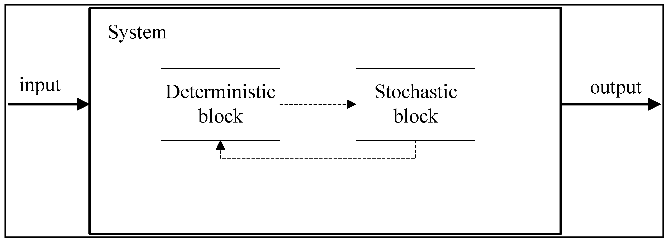
When implementing the hybrid-pair approach for renewable power plants, the energy transformation process can be broken down in two models, as shown in Figure 1: the deterministic block defines the energy transformation performed by a renewable power plant and the stochastic block models the system failure logic.

Among the possible approaches, the one based on Stochastic Automaton [24,25,26,27] can be coded and simulated to satisfy all the criteria mentioned in Table 1. For this reason, the Stochastic Hybrid Fault Tree Automaton (SHyFTA) [25] is chosen as a suitable modelling formalism and the main steps for the design of a SHyFTA model for a renewable power plant are summarized. In this work, the Matlab-Simulink framework (The MathWorks, Natick, MA, United States) has been used, because it offers a friendly graphical user interface that allows easy design, coding and debugging the model.

The application of the proposed approach is discussed with the aid of a case study on a real photovoltaic power plant to quantify the energy production throughout the entire power plant lifetime and compare it with the one provided using a pure deterministic model (Figure 1).

The rest of this paper is organized as follows. Section 2 introduces the theoretical background of Stochastic Hybrid Fault tree Automaton. In Section 3 the case study is discussed and Section 4 presents the simulation framework offered by the Matlab-Simulink to implement the SHyFTA model and run the simulations. Finally, Section 5 summarizes conclusions and discusses future work.

2. Stochastic Hybrid Fault Tree Automaton: Concept and Implementation in Renewable Power Plants

The mathematical formulation of SHyFTA is presented in [25], therefore interested readers can refer to it for further information. A SHyFTA model is made up of a deterministic and a stochastic process.

The deterministic process is expressed in terms of a set of ordinary or partial differential equations, whereas the stochastic process is built up using the Dynamic Fault Tree formalism [28,29].

Wearing-out of components is modelled using a Weibull pdf (probability density function) with shape factor β > 1 (i.e., the failure rate is increasing with respect to time):

$$\mathsf{\lambda }\left(\mathrm{L}\right)=\mathsf{\beta }/\mathsf{\gamma }·{\left(\mathrm{L}/\mathsf{\gamma }\right)}^{\mathsf{\beta }-1}$$

(1)

The non-linear variable L(t) of Equation (1) represents the component aging. It can be computed solving the Deterministic Piecewise Markov Process [30], described with the differential equation Equation (2) [31,32], where i_on is the piecewise discrete variable assuming value 1 if the component is switched on and 0 if it is switched off.

$$\frac{\mathrm{dL}\left(\mathrm{t}\right)}{\mathrm{dt}}={\mathrm{i}}_{\mathrm{on}}\mathrm{where}{\mathrm{i}}_{\mathrm{on}}=\{\begin{array}{c}1,\mathrm{if}\mathrm{the}\mathrm{component}\mathrm{is}\mathrm{switched}\mathrm{on}\\ 0,\mathrm{if}\mathrm{the}\mathrm{component}\mathrm{is}\mathrm{switched}\mathrm{off}\end{array}$$

(2)

This last relationship allows a more realistic wearing-out of a component because the age L in Equation (2) increases only when the component is working.

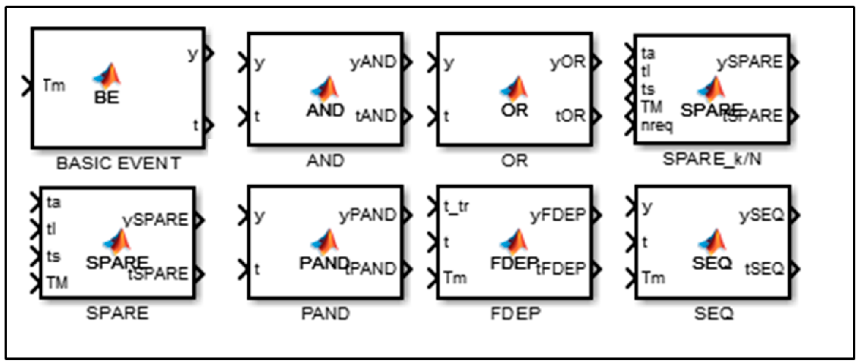
In a SHyFTA, the stochastic process is described by a Dynamic Fault Tree (DFT) model, a well-known technique of reliability engineering able to model complex time-dependent interactions among the components of a system. DFT has gained the interest of researchers and risk practitioners thanks to the graphical formalism constituted by Boolean gates and the powerful set of dynamic gates shown in

Table 3. Dynamic gates of Dynamic Fault Tree.

Name	Graphical Representation	Description (N Input)
SPARE		It triggers only after the primary and all the N-1 spare occur. Spares can be shared with other spare gate. It is possible to identify three different types of spare on the basis of the dormancy factor α which is a multiplicative factor to the active failure rate (when the spare is not in use): Cold: α = 0, spare cannot fail as long is not active; Hot: α = 1, spare can fail at the same rate as when active; Warm: 0 < α < 1, spare can always fail, but at a reduced failure rate when is not in use.
PAND		It behaves like an AND gate but it triggers only if the input events occur in the order from the leftmost to the rightmost.
SEQ		It forces the input events to occur from the left to the right order. It can model the gradual degradation of a system. It behaves as a Cold Spare Gate.
FDEP		This gate models the failure of the dependent input events if the trigger occurs. The output is a dummy or an input for other gates. Note that input events can fail by themselves too.

[33]. The design of a Dynamic Fault Tree starts with the definition of a top-event that represents an undesired scenario of the system. Following a top-down procedure, the causes of the top-event must be identified and analyzed in order to the combinations that determine the top-event occurrence. The combination logics are expressed using the gates that take in inputs the intermediate and the basic events. These latter generally correspond with the system component fault and cannot be further decomposed.

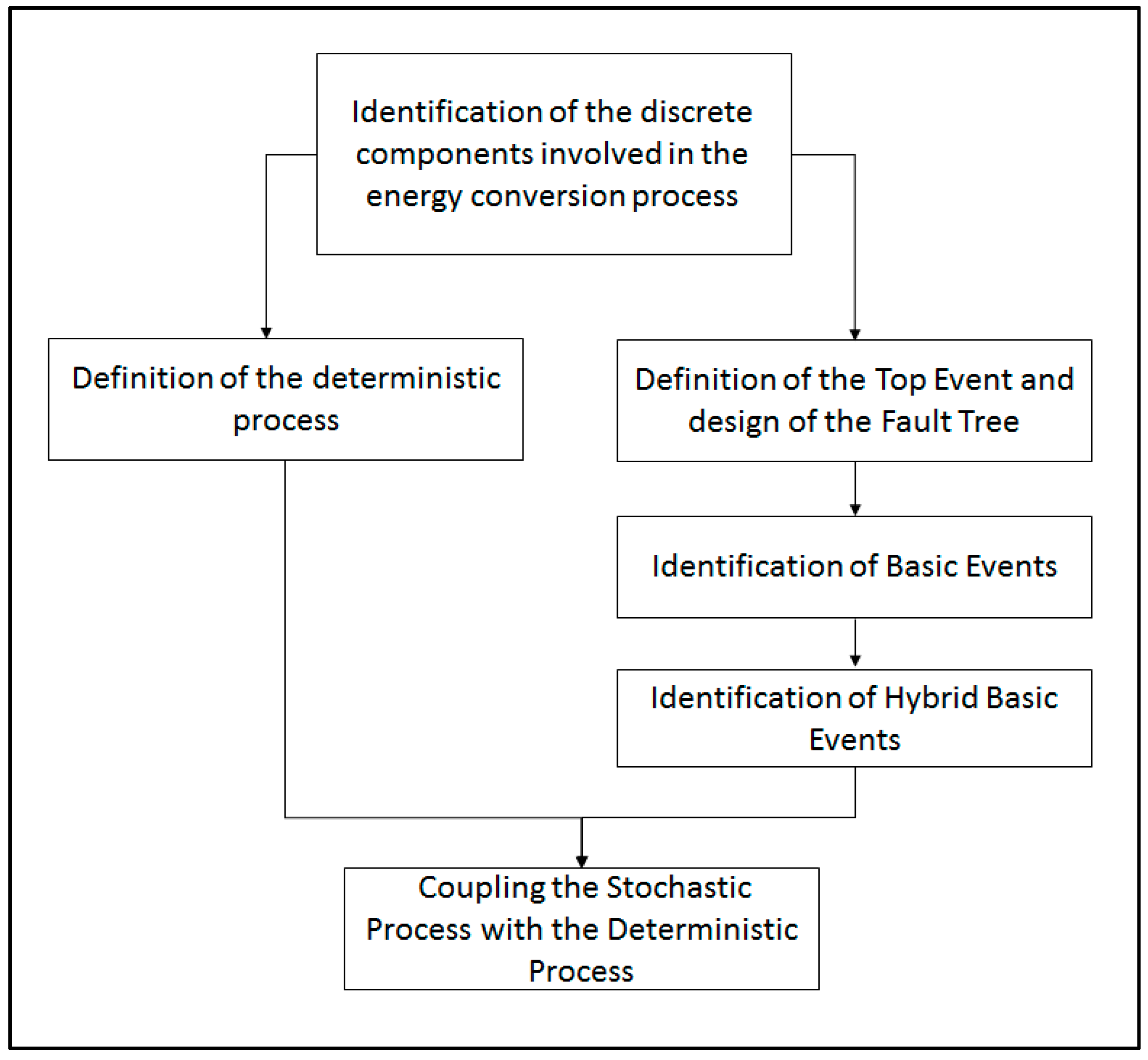
A SHyFTA model can be realized following the procedure shown in Figure 2. In the first step, the discrete components that are involved in the energy conversion process of the power plant must be identified. The computational complexity of the deterministic model basically depends on the accuracy and the number of interactions presented in the model. The mathematical equations should describe the contribution of each component at different working regimes.

The main input of the deterministic process is the time-series of the primary renewable resource. Generally, these information are obtained with a site assessment and can be refined registering the meteo data for several years in order to enrich the statistical sample to use in the model.

The discrete components identified in the study of the renewable power plant must have a counterpart in the stochastic fault tree model. In this way, any variation of the health and of the operating conditions of the components affects the failure behavior and the performance of the system. For the fault tree model, it is important to identify a top-event, representing an undesired operational condition of the system and its elementary causes, the so-called basic events. Basic events must be combined together by the use of temporal and logic gates (AND, OR, VOTING k/N, PAND, SPARE, FDEP, SEQ) and they can be repeated (i.e., they appear two or more times in the fault tree as inputs of two or more different gates) although they represent a unique event within the real system.

The main stochastic inputs of a SHyFTA model are the probability density functions (pdf) of the components of the fault tree. When a component is modelled with a hybrid basic event, the pdf is not static and, in this case, a set of different pdf must be defined. Although the complete shutdown of a renewable power plant consisting of several generating units is very unlikely, the modelling of this scenario as the Top Event of the fault tree allows the evaluation of several performance indicators. Among them, the instantaneous active and reactive power, the energy production within a time-period and the service availability that corresponds with the probability of the renewable power plant to produce a base power and guarantee the continuity of service [8,34] for a well-defined demand curve. These key performance indicators (KPI) can provide important indications for suitable dimensioning of the power plant and the life cycle activities like production plans and the maintenance schedule.

The formulation of the SHyFTA is completed when the stochastic and the deterministic models are coupled through shared variables. A typical example of coupling is the failure of a component (in the stochastic model) that nullifies the contribution of the same component within the deterministic process (e.g., an inverter that fails will no longer output AC power). Other possible couplings can link the operational conditions of a component with its health status and failure behavior.

3. Case Study: A Photovoltaic Power Plant

There have been proposed different fault tree models of renewable power plants that can be used as reference models to build up a SHyFTA [12,13,14,15,16,17,18]. In this paper, the case study of a photovoltaic power plant is presented.

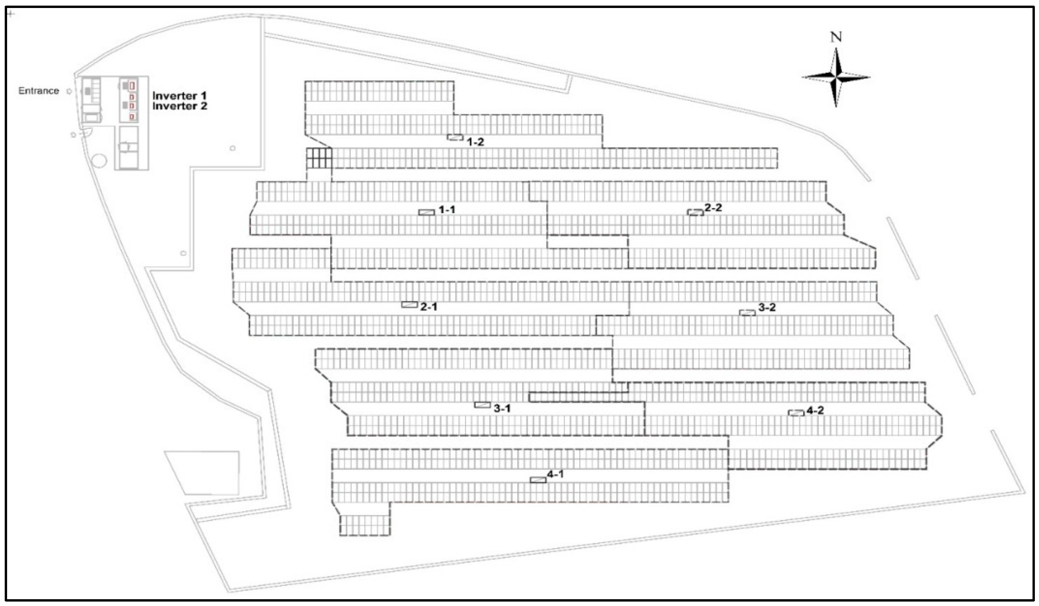
The analyzed power plant is a grid-connected photovoltaic power plant with no trackers implemented by a private company in 2011, located in Sicily (37.1751° N 16.1596° E) close to Syracuse (see

Table 4. PV system characteristics.

Location	37.1751° N 16.1596° E
Ppeak	419.52 kWp
N° inverters	2
N° strings boxes	4 (for inverter)
N° strings	138
N° modules	2208 (16 for each string)
Azimuth Angle (β)	180°
Tilt	30°

).

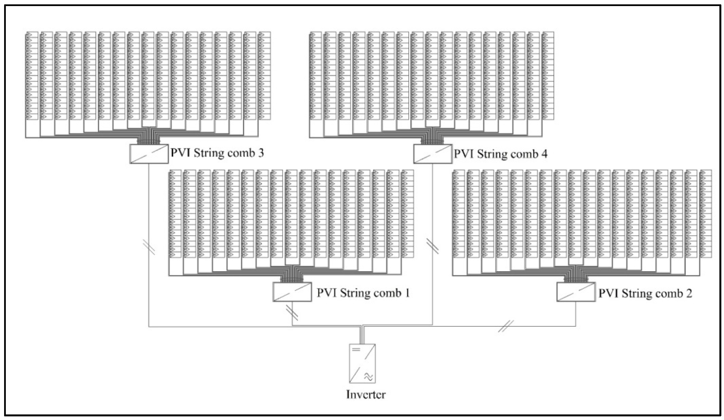
The power plant is characterized by a peak power, P_peak = 419.5 kW and by two identical DC/AC inverters of 220 kW_p. There are 4 string boxes for each inverter: 3 accomodate 17 strings and 1 accomodates 18 strings. The strings are connected in parallel while the modules are in series (Figure 3 and Figure 4). Table 4,

Table 5. PV module main characteristics.

Ppeak	190 W (Monocrystalline)
Panel efficiency (η)	15%
Vmp	37 V
Imp	5.04 A
Voc	45.1 V
Isc	5.35 A
NOCT	45 ± 2 °C

and

Table 6. Inverter mail characteristics.

Pacmax	220 kW
Voltage range MPPT	485 V < VMPPT < 950 V
N° independent MPPT	4
ηmax	98%
Vacr	320 V
Iacmax	450 A
Idcmax	492 A

summarize the main characteristics of the system.

To be compliant with the Italian Producer Electrical Regulation (IPER) of 2011, known also as Terzo Conto Energia [35], the power plant is connected to the national grid and the energy production is 100% devoted to the grid. The IPER states that the power plant must stop in case of disconnection from the national grid and forbids the use of energy storage systems. There is a strong economic advantage for adhering to the IPER of 2011. In fact, for the first 20 years of life of the power plant, there is a fixed economic subsidy for all the energy produced. Moreover, the energy not instantaneously consumed by the producer is tracked and sold with a price dictated by the energy market. Therefore, the power plant contributes to the company activities by supplying the internal consumption and providing a profit due to the economic incentive (subsidy) and the sale of the energy not consumed.

Table 7. IPER 2011 Subsidy. Price * is based on an average value of the energy price in the energy market (2011) [35].

Power (kW)	Subsidy	Price *	Total (∑)
1 < P ≤ 3	0.362	0.25	0.612
3 < P ≤ 20	0.339	0.21	0.549
20 < P ≤ 200	0.321	0.18	0.501
200 < P ≤ 1.000	0.314	0.15	0.464

* Apex of Price.

shows the value of the Subsidy (it is fixed by the IPER [35]) and the corresponding price of buy/sell per one kWh of energy. This latter is a rough value of the energy price in the energy market (2011). The column Total is the sum of the previous contributes and it is used to estimate the payback generated by the energy produced by the power plant.

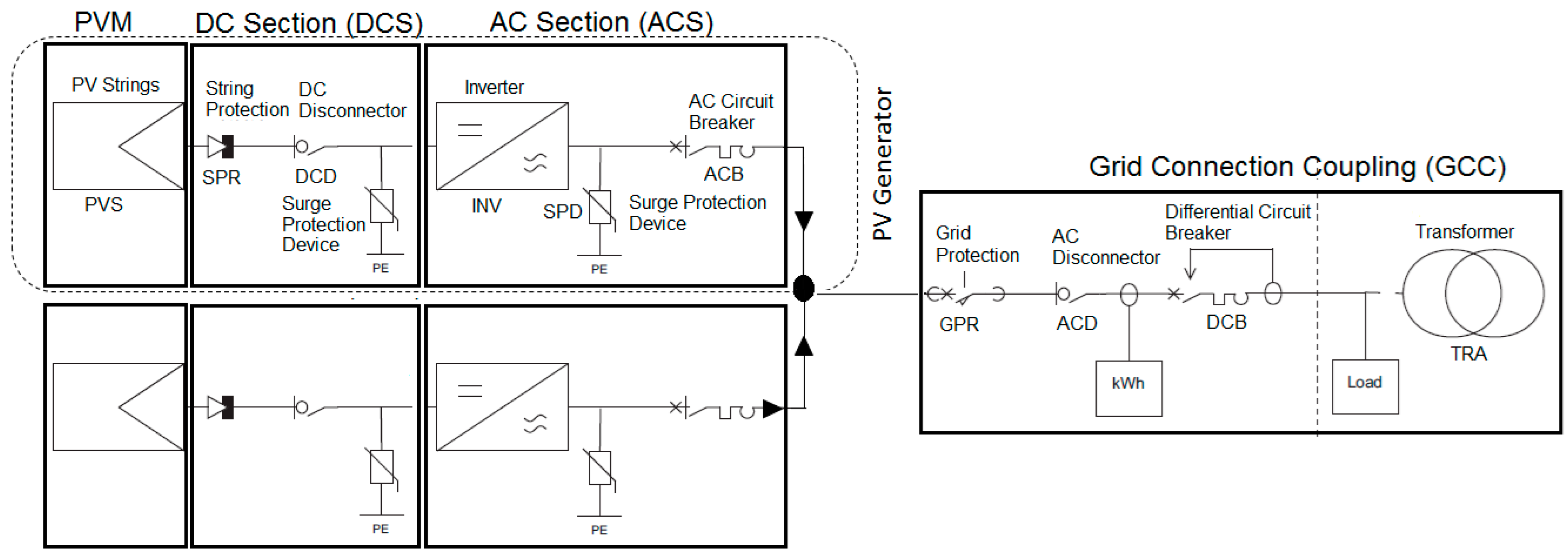
With reference to Figure 3 and Figure 4 it is possible to identify the main components of the photovoltaic power plant.

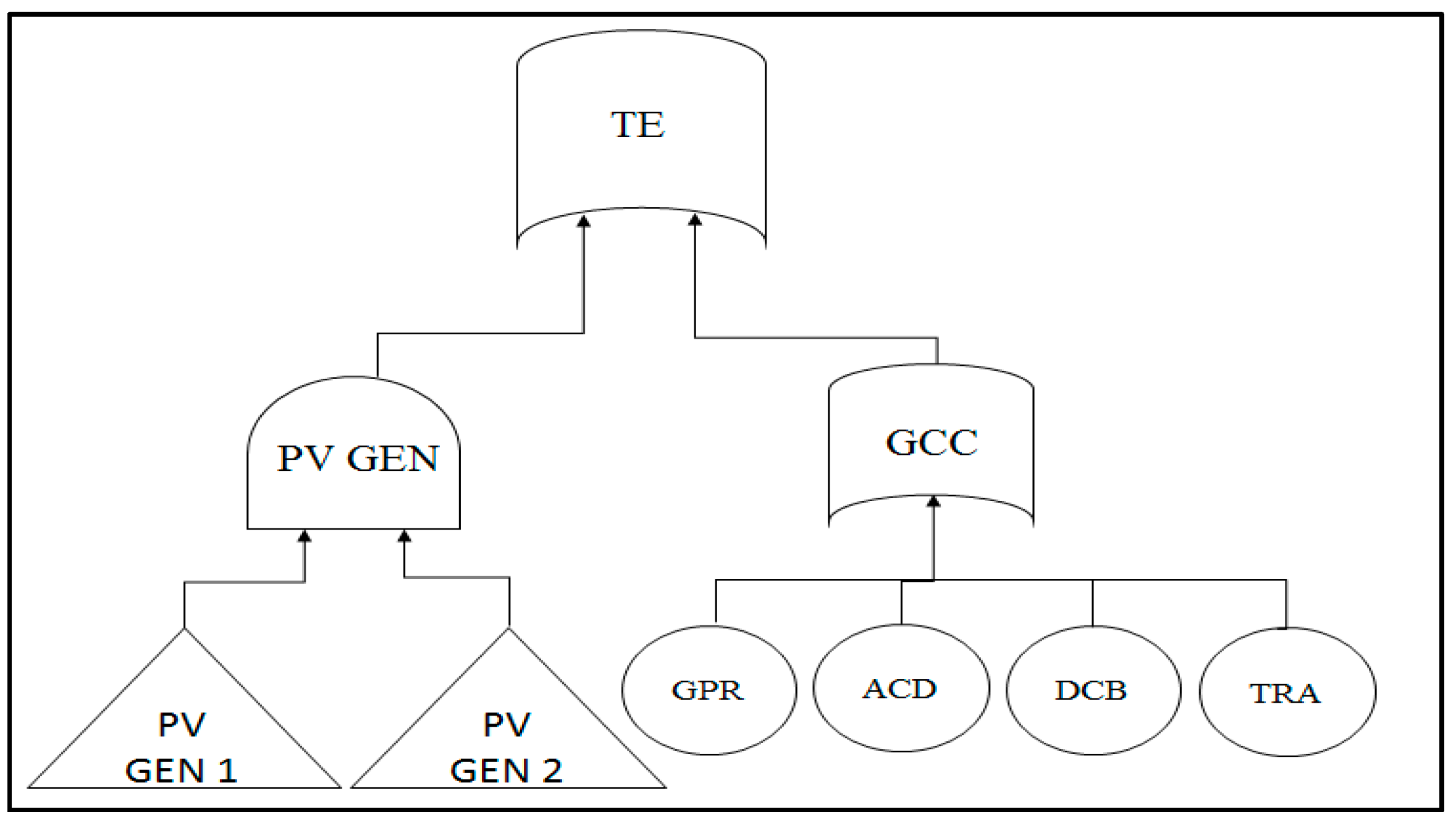
The components of the photovoltaic power plant can be grouped into the following functional blocks (Figure 5):

• PV Module (PVM), constitutes the PV module strings of the power plants (PVS);
• Direct Current Section (DCS), made up of string protection diodes (SPR), DC disconnectors (DCD) and surge protection devices (SPD);
• Alternating Current Section (ACS),made up of inverters (INV), surge protection devices (SPD) and AC circuit breakers (ACB);
• Grid Connector Coupling (GCC), made up of grid protection (GPR), an AC disconnector (ACD), a differential circuit breaker (DCB) and a transformer (TRA).

Next we apply the steps discussed in Section 2 to build up the SHyFTA model.

3.1. Definition of the Deterministic Process

The photovoltaic conversion starts in the PVM stage where PV modules capture the solar irradiance that is converted into a DC power. They are organized in electrical strings connected in series and parallel to constitute a panel. In the same manner, several panels are connected to form arrays of generators and sum up to a higher direct current (DC) power.

As a first approximation, the electrical power generated with a simple configuration (same tilt and orientation for all modules/strings) [36] can be defined as follows:

$$\mathrm{P}={\mathsf{\eta }\mathrm{I}}_0\sin \left(\mathsf{\alpha }\right)\mathrm{S}$$

(3)

where I₀ is the orthogonal solar irradiance to the direction of solar radiation [W/m²]; α is the angle of the module/string with respect to the incident solar radiation; S is the area of the module [m²]; and ƞ is the system efficiency that is always less than 1.

The total efficiency can be expressed as:

$$\mathsf{\eta }={\displaystyle \prod }_{\mathrm{i}=0}^{\mathrm{n}}{\mathsf{\eta }}_{\mathrm{i}}$$

(4)

where n is the number of loss effects considered at each ith stage of the power plant.

At the PVM stage, meteorological factors (e.g., wind speed, cloud transients in PV units, incident irradiance or ambient temperature) or yearly deterioration can reduce the efficiency of the photovoltaic modules. Using Equation (3) we can compute the efficiency of the module, η_m, by considering the variation of the temperature [37]:

$$\{\begin{array}{l}{\mathsf{\eta }}_{\mathrm{m}}={\mathsf{\eta }}_{\mathrm{std}}\left\{1-\mathsf{\rho }\left({\mathrm{T}}_{\mathrm{c}}-{\mathrm{T}}_{\mathrm{c},\mathrm{std}}\right)\right\}\\ \frac{{\mathrm{T}}_{\mathrm{c}}-{\mathrm{T}}_{\mathrm{a}}}{\mathrm{G}}=\mathrm{constant}\end{array}$$

(5)

where η_std and T_c,std are respectively the efficiency and the module temperature at standard conditions, ρ is the power coefficient (percentage variation of power for 1 °C), T_c and T_a are the module and ambient temperatures and G is the global irradiance on the module.

To account for the degradation rate, Dr, corresponding with the percentage of efficiency lost every year [38], it is possible to use a linear equation model:

$${\mathsf{\eta }}_{\mathrm{n}}={\mathsf{\eta }}_{\mathsf{\eta }\mathrm{first}}\left(1-{\mathrm{nD}}_{\mathrm{r}}\right)$$

(6)

where η_first is the nominal efficiency at the first year, while η_n is the efficiency calculated at the nth year.

The performance degradation occurring in the PVM stage reduces the DC power, but does not stop the power production unless the DC breakers and disconnectors of the DCS stage interrupt the circuit or the cables fail. In fact, with reference to Figure 6, a single PV generator can contribute to the power generation of the system if the circuit path from the PVM stage to the GCC is closed.

Before connecting to the grid, the DC current is converted in alternating current. The DC/AC inverter of the AC section performs this transformation with an efficiency that depends on the input load. At this stage, inverters can also affect the performance of the system [39] and the algebraic model presented in [40,41] illustrates this effect:

$${\mathsf{\eta }}_{\mathrm{ACS}}=\frac{\mathrm{P}{\left(\mathrm{t}\right)}_{\mathrm{AC}}}{\mathrm{P}{\left(\mathrm{t}\right)}_{\mathrm{DC}}}=1-\frac{\mathrm{P}{\left(\mathrm{t}\right)}_{\mathrm{loss}}}{\mathrm{P}{\left(\mathrm{t}\right)}_{\mathrm{DC}}}$$

(7)

The total power of the plant is the sum of the AC powers of the two PV generators:

$${\mathrm{P}}_{\mathrm{GCC}}\left(\mathrm{t}\right)={\mathrm{P}}_{\mathrm{ACS}1}\left(\mathrm{t}\right)+{\mathrm{P}}_{\mathrm{ACS}2}\left(\mathrm{t}\right)$$

(8)

For this reason, it is possible to understand that the photovoltaic plant is able to produce energy if at least one of the two PV generators is in operation. To compute the energy produced and measured by the generation meter (GM) in the GCC stage it is possible to integrate the PGCC in the time interval [t2, t1]:

$${\mathrm{E}}_{\mathrm{GM}}\left(\mathrm{t}\right)={{\displaystyle \int }}_{\mathrm{t}1}^{\mathrm{t}2}{\mathrm{P}}_{\mathrm{GCC}}\left(\mathrm{t}\right)\mathrm{dt}$$

(9)

The other components involved in a photovoltaic system are protection, cables, breakers, disconnectors and transformers. These components all play an important role in the energy production because if one of them interrupts the circuit path to the GCC, the PV generator in the open path cannot contribute to the power generation. A more critical condition occurs if the circuit path stuck open inside the GCC stage. In this case, all the power plant has to stop the production because it gets disconnected from the national grid, causing the complete system unavailability. To address these circumstances, the stochastic fault tree model, object of the next subsection, has to be designed.

3.2. Definition of the Stochastic Process

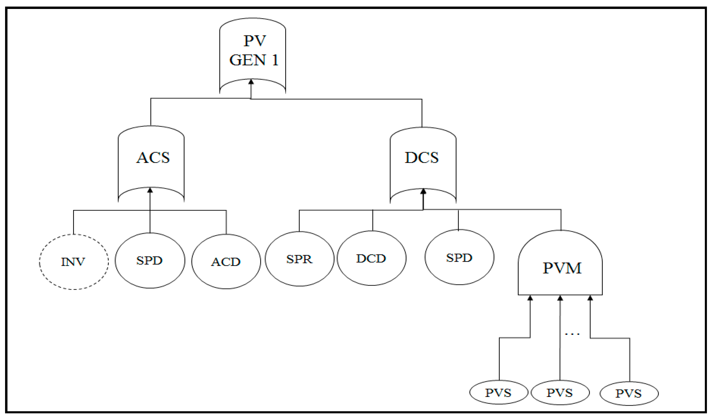
The fault tree model in Figure 6 describes the failure behavior of the plant. This model is constituted by an OR gate (TE) that takes as input an OR gate (GCC = OR (GPR, ACD, DCB, TRA)) and an AND gate (PV GEN = AND (PV GEN 1, PV GEN 2)), modelling the failure behavior of the PV generators. The plant production unavailability occurs if both PV generators fail or if one of the components of the GCC fails. Figure 7 shows the failure behavior of a single PV generator. The failure/repair rates of the components are shown in

Table 8. Failure/repair rates and steady state availability of the components of the PV plant.

Component		λ: Failure Rate [h−1]	µ: Repair Rate [h−1]
PVS	PV Strings	2.43 × 10−5	2.3 × 10−4
SPR	String Protection	0.313 × 10−6	2.08 × 10−2
DCD	DC Disconnector	0.2 × 10−6	2.08 × 10−2
SPD	Surge Protection	0.313 × 10−6	2.08 × 10−2
ACB	AC Circuit Breaker	5.71 × 10−6	2.08 × 10−2
GPR	Grid Protection	5.71 × 10−6	2.08 × 10−2
ACD	AC Disconnector	0.034 × 10−6	2.08 × 10−2
STB	String box	0.015 × 10−3	2.08 × 10−2
DCB	Diff. Circuit Breaker	5.71 × 10−6	2.08 × 10−2
TRA	Transformer	1.4 × 10−6	2.28 × 10−4
INV	Inverter	Aging Weibull	1.7 × 10−3

. Failure rates have been taken from [12]. Note that the inverter has been modeled as a hybrid basic event using a Weibull distribution whose failure parameters depend on the aging variable that, in turn, is bounded to the solar radiation of the deterministic process. In fact, the inverter is in mode on when the DC voltage produced from PV strings is high enough to make it work, and obviously these PV strings produce energy accordingly solar radiation. Otherwise, the inverter stays in stand-by mode, waiting for the sun irradiance to increase (e.g., during the night time).

As for repair rates, it was assumed that electrical components like breakers, disconnectors, string box and protection can be restored to as-good-as-new within two working days after a fault.

According to the agreements with the inverter manufacturer, the repair of the inverter takes between three and four weeks, considering the whole process of inspection, ordering, delivery and replacement. For the PV strings it was assumed a periodic inspection would take place every six months.

4. Simulation of the SHyFTA Model

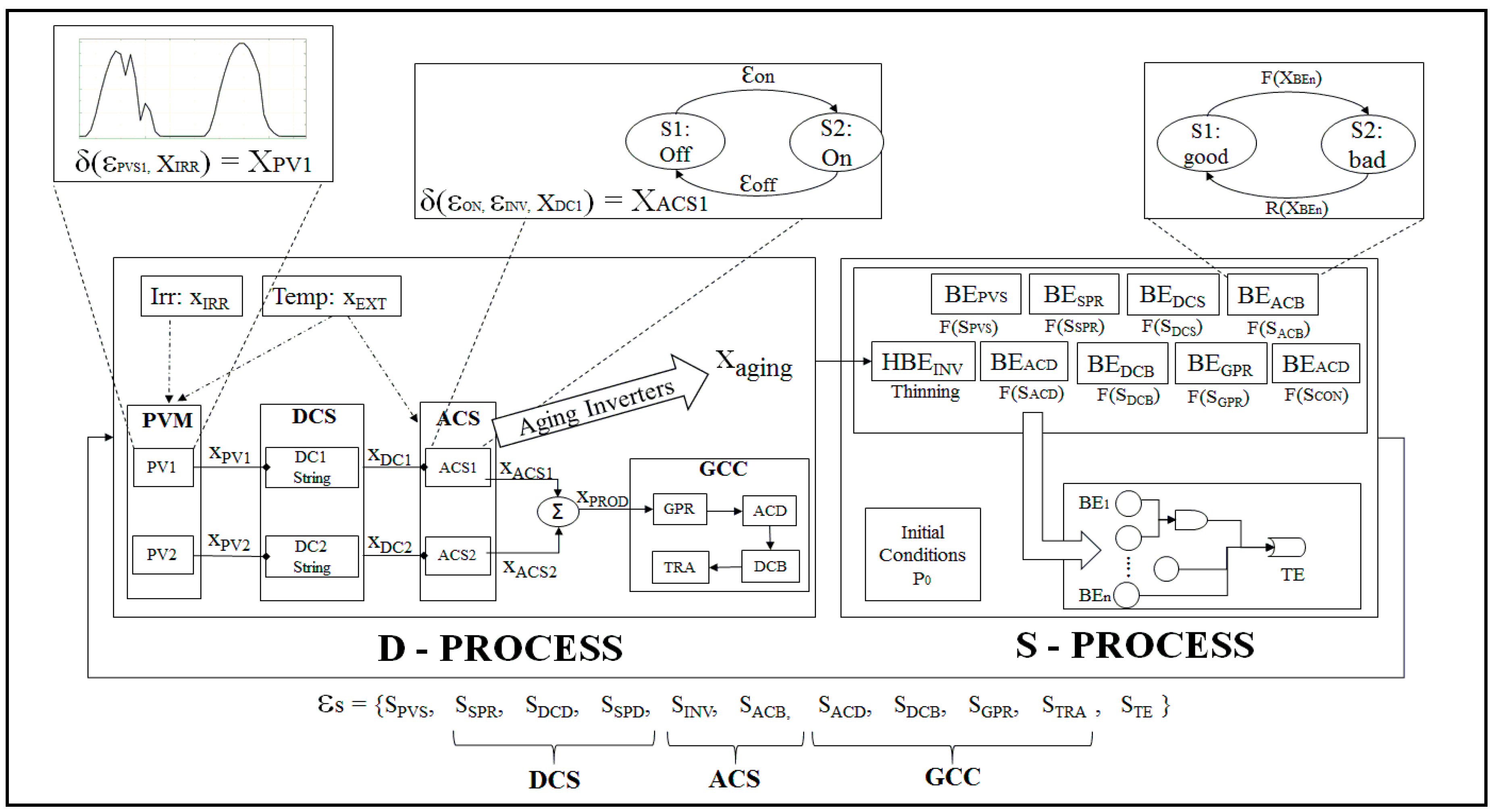
Figure 8 depicts the hybrid-pair model of the case study with the corresponding mapping into a SHyFTA.

It is possible to identify the main discrete components of the PV system and the corresponding variables, respectively Xi and Ɛi, of the deterministic and stochastic processes. The variables X_PV1/2, X_DC1/2, X_ACS1/2 and X_PROD are the powers generated at the different stages of a PV generator. X_IRR and X_EXT represent respectively the sun irradiance and the external temperature of the environment. These two variables are inputs of the model and, according to Equations (3)–(6), affect the power generation and the conversion efficiency of the PVM components. Randomness of these input is achieved exploiting the historical data series of the last five years retrieved by the SCADA of the power plant. For each iteration of the Monte Carlo simulation process, the value of X_IRR and X_EXT of the ith hour of the day is fixed extracting a random value in the uniform range between the minimum and maximum value of the corresponding ith hour of the day. The ACS conversion depends on Equation (7) and the actual energy produced by the power plant is described by Equations (8) and (9).

Among the variables computed in the deterministic process, X_aging = L is the time input of the Weibull pdf characterizing the failure behavior of the inverter in the stochastic process (see Equation (2)).

In the stochastic process, the basic events are characterized with two operational states, S_S = {Good, Bad}. The health status of each basic event is an element of the vector Ɛ_S that, as input of the deterministic process, realizes the coupling between the basic event of the stochastic process and its corresponding discrete component modelled in the deterministic process.

The SHyFTA model has been coded in Matlab and Simulink to implement a software resolution of the hybrid-pair model based on a discrete event Monte Carlo simulation [42]. The Matlab scripts perform the computation related with the global variables of the simulation, including the stopping logic algorithm of the Monte Carlo simulation. The Simulink program is used to create the hybrid-pair model because both the deterministic and the stochastic process can be assembled with the built-in blocks available in the Simulink library. As for the dynamic gates, the MatCarloRE [43] library can be used (Figure 9).

The Matlab ‘Initialization Script’ (

Table 9. The initialization script implemented in Matlab.

Initialization Script
# Initialization of global setting. The variables are used within the Hybrid-Pair model in Simulink
1: InitHS(); # call a method that load and randomize the input historical series
2: InitDP(); # call a method to initialize the parameters used in the Simulink deterministic block
3: InitSP(); # call a method to initialize the parameters of the Basic Events in the Simulink stochastic block
4: iter = 0; # Monte Carlo iteration counter
5: N_ITER = 1000000; #max number of iterations
6: estimator = 0; # global variable to adopt as estimator
7: iterEstimator = 0; # variable to adopt as estimator within the nth iteration
8: error = 0; # global variable to adopt to evaluate the error
9: alfa_conf = 0.99; # is the confidence level used to evaluate if the error is within the confidence interval
10: missionTime = 40173; # the unit of measure (hours) has to be the same of the failure/repair rates
11: deltaT = 1; # this corresponds with the integration-step (in hours) of the simulation process
12: bdroot = ‘hybrid_pair_1’; # this variable handles the Simulink hybrid-pair model that starts the simulation
13: set_param (bdroot,’SimulationCommand’,’Update’); #this command updates the variables of the Simulink models that are set in the Matlab scripts
14: set_param (bdroot,’SimulationCommand’,’Start’); #this command gives the control to the Simulink engine and restart the simulation

) to set up the parameters of the SHyFTA simulation is shown in Table 9 and is launched one time to start the simulation process. Lines (1–3) are configurable methods that must contain the parameters of the simulation. The InitHS() load the historical data series and perform a randomization process so as to vary these input data at each iteration of the Monte Carlo simulation. The InitDP() initializes the parameters of the Deterministic Process, like unit conversion factors (if needed), physical constants and variables (that may vary during the iteration) and so on. The InitSP() initializes the corresponding failure and repair rates used in the Simulink blocks of the Stochastic Process to characterize the Basic Events of the Fault Tree. Moreover, for each Basic Event, this method computes the time of failure of the corresponding component using the inversion law t = F⁻¹(λ). Note that for the Hybrid Basic Events of the inverters, variable failure rates are updated during the simulation of an iteration in order to consider the variation of the aging variable. From lines (4–11), the other variables required for the Monte Carlo simulation are initialized and line (12) sets the name of the Simulink model (which corresponds with the .slx file) that will be called at the beginning of the simulation (in our code it is named ‘hybrid_pair_1’). With line (13) the variables initialized with the Matlab script are passed to the Simulink environment and line (14) starts the simulation.

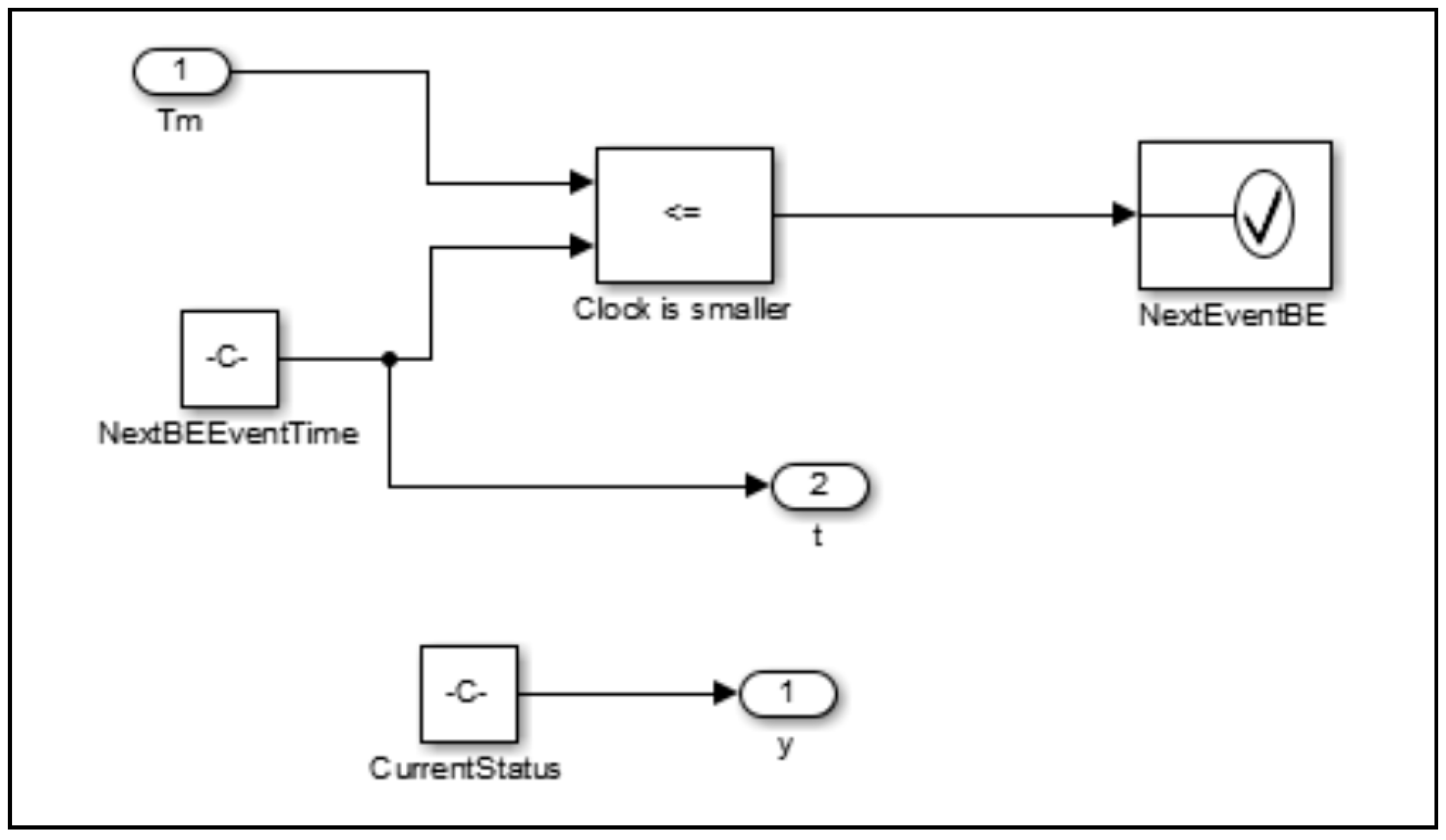
When the simulation starts with the first iteration, the time variable of the Simulink (Ts) increases according to the step of integration (deltaT), so that Ts = Ts + deltaT. Meanwhile, the Deterministic Block performs the computation of the equations Equations (3)–(9), whereas the Basic Events of the Stochastic Block updates the status of its corresponding component only when Ts reaches the time of failure of the corresponding Basic Event. This behavior is obtained using an assertion block (see Figure 10) inside the Basic Event block that calls the method NextEventBE() in case the assertion condition is verified.

The NextEventBE() method is shown and commented in

Table 10. The NextEventBE script implemented in Matlab.

NextEventBE Script
1: set_param(bdroot,’SimulationCommand’,’Stop’);
2: if (currentStatus == 1) #the status of the Basic Event has been GOOD until the assertion raised
3:    currentStatus = 0; # update the status neglecting the GOOD
4:    nextBEEventTime = InvertRepairDistribution(repairRate); # find the next repair time
5: else
6:    currentStatus = 1; # update the status neglecting the BAD
7:    nextBEEventTime = InvertFaultDistribution(failureRate); #find the next failure time
8: end
9: set_param (bdroot,’SimulationCommand’,’Update’); #this command updates the variables of the Simulink models that are set in the Matlab scripts
10: set_param (bdroot,’SimulationCommand’,’Start’); #this command gives the control to the Simulink engine and start the simulation of the first iteration

.

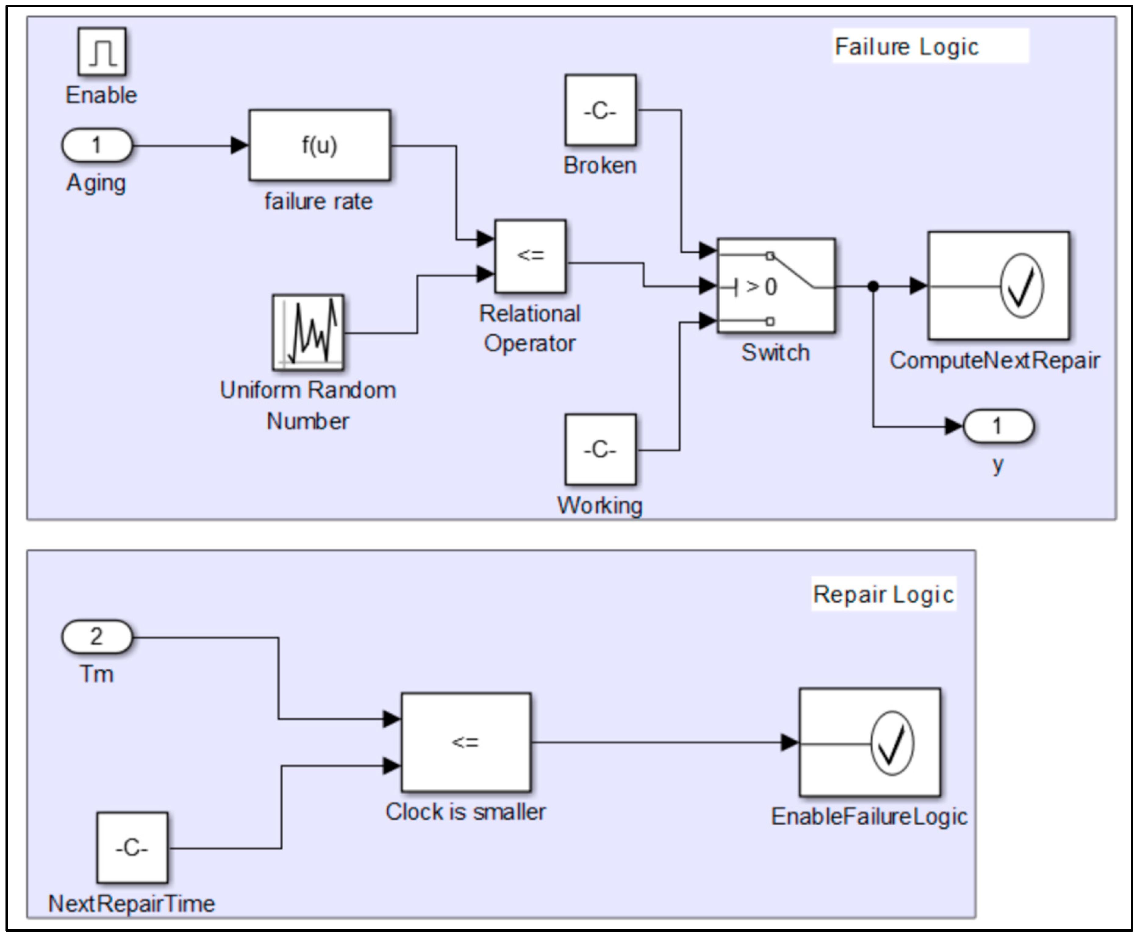
As for the Hybrid Basic Events, the Simulink block is different and is shown in Figure 11.

The Hybrid Basic Event block requires a complex logic able to evaluate at each step of the iteration (for each deltaT) the status of the component. This is performed in the Failure Logic where the function ‘failure rate’ takes as input the aging and the characteristic parameters of the probability density function of the component in order to evaluate if the component is failed or working. This last logic is realized comparing the instantaneous probability of failure with a random number in [0, 1]. If the output of the f(u) function is smaller than the uniform random number the component has failed and the Failure Logic block raises the ComputeNextRepair() function inside the corresponding assertion block. Notice that the Failure Logic block has an enabling condition that is modified to False by the ComputeNextRepair() function when the component gets failed. Moreover, the ComputeNextRepair() computes the next time of restoration and passes the control to the Repair Logic block that works with the same logic of the normal Basic Event block.

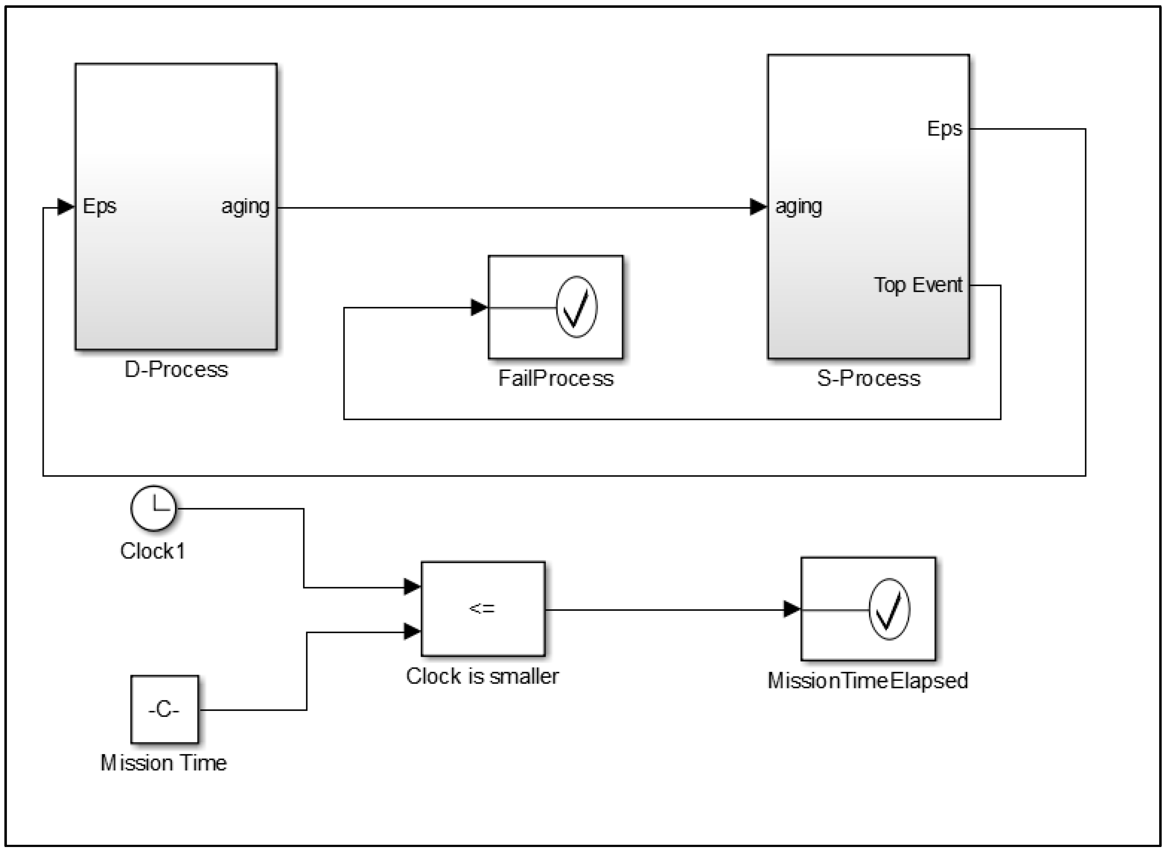
Figure 12 shows the highest-level Simulink block of the hybrid-pair model that constitutes the SHyFTA of our case of study. It is possible to identify the shared variables between the deterministic and the stochastic processes, where Eps is the vector that contains the statuses of all the Basic Events of the photovoltaic power plant, Top Event is the output of the Fault Tree and the aging variable is the real-time variable that is computed in the deterministic process (using an integrator block) solving Equation (2) and that is passed to the stochastic process to evaluate the dynamic failure rate of Equation (1). Several trials must be performed in order to bind with the desired accuracy (or confidence interval) the estimator of the measure to compute. In order to run multiple times a Simulink model, an assertion block that controls the elapsing of the mission time must be added. This assertion block is activated as soon the clock of Simulink reaches the mission time Tm. It invokes a Matlab script that handles the transition to another Monte Carlo iteration. The instructions of the Matlab script invoked by the block MissionTimeElapsed are resumed in

Table 11. The MissionTimeElapsed script in Matlab.

MissionTimeElapsed Script
# Initialization of global setting. The variables are used within the Hybrid-Pair model in Simulink
1: if (iter<N_ITER)
2:   set_param(bdroot,’SimulationCommand’,’Stop’)
3:   UpdateGlobalVariables();
4:   completed = VerifySimulationAccuracy();
5:     if (completed==0)
6:        iter = iter + 1;
7:        iterEstimator = 0;
8:        if (iter%2==1) # select the Simulink hybrid_pair model of the next iteration
9:          bdroot = ‘hybrid_pair_2’;
10:       else
11:          bdroot = ‘hybrid_pair_1’;
12:        end
13:        InitSP(); # initialize the parameters of the Basic Events in the Simulink stochastic block
14:        InitDP(); # initialize the parameters used in the Simulink deterministic block
15:        InitHS(); # load and randomize the input historical series
16:        iterEstimator = 0; # reset the estimator for the next iteration
17:        set_param (bdroot,’SimulationCommand’,’Update’);
18:        set_param (bdroot,’SimulationCommand’,’Start’);
19:     else
20:        disp (‘Simulation Completed. Accuracy required reached’);
21:     end
22: end
23: disp (‘Simulation over. Accuracy required not reached’);

.

In particular, the script stops the Simulink simulation (line 2), updates the global variables and the estimator of the Matlab workspace (with the method UpdateGlobalVariables()) using the information generated in the Simulink environment (line 3) and verify if the accuracy required by the Monte Carlo setting is reached (line 4). If the variable ‘completed’ is not True (=1), lines (6–18) resets the simulation parameters to prepare for a next iteration. Before calling the built-in method of Simulink ‘set_param’ (line 17) to update the Simulink workspace for a new iteration, an important setting has to be performed (lines 8–12). In fact, Simulink cannot restart the simulation of the model that has stopped. In other words, a Simulink model cannot trigger its own restart. In order to overcome this issue, the final Simulink implementation requires a couple of identical model that alternate each other, at any iteration. In our case study, they are respectively named, ‘hybrid_pair_1’ and ‘hybrid_pair_2’, corresponding with two different “.slx” Simulinkfile models. The global variable ‘bdroot’ is used to alternate these two identical Simulink models. Finally, in line 17, the Monte Carlo simulation is started again for another iteration.

For the photovoltaic power plant, we are interested in the active power production measured at the generation meter, P_GCC. Therefore, at each trial k of the Monte Carlo simulation, the output of the SHyFTA model is the time-series P^k_GCC(t). This last variable is updated in the method UpdateGlobalVariables(). When the desired confidence interval is met the simulation is stopped and the mean active power for each sample of the time series is computed as follows:

$$\mathbb{E}\left[\left({\mathrm{P}}_{\mathrm{GCC}}\right)\right]=\frac{1}{\mathrm{N}}\left[{\displaystyle \sum }_{\mathrm{k}=1}^{\mathrm{N}}{\mathrm{P}}_{\mathrm{GCC}}^{\mathrm{k}}\left(\mathrm{t}\right)\right]$$

(10)

where N is the number of Monte Carlo trials so far completed.

The estimator error associated to the desired confidence interval can be computed as follows [44]:

$$\mathrm{Err}={\mathrm{Z}}_{\mathrm{a}/2}\times \frac{\mathsf{\sigma }}{\sqrt{\mathrm{N}}}$$

(11)

where Z_a/2 is the confidence coefficient, a is the confidence level, σ is the standard deviation of the Monte Carlo simulation and N is the number of Monte Carlo trials.

The use of the active power as an estimator of the Monte Carlo simulation has an advantage. In fact, it can be noted that the cumulative error, made up by the instantaneous samples of the time series P_GCC(t), corresponds to an energy. In this way, it is possible to provide an appropriate estimation of the active energy aside a confidence interval using the cumulative error of the estimator.

Energy Production Estimation

In order to test the accuracy of the proposed methodology, the results of the SHyFTA and the deterministic models have been compared with the real data of energy production, collected by the SCADA system of the photovoltaic plant at the time these data were provided. The collected data includes the hourly aggregated power, energy, solar irradiance and external temperature for the first four years and half of life, corresponding to 40,173 h.

For the SHyFTA simulation, a confidence level of 0.99 was set for each data point P_GCC(t). There was not any stopping condition set for the simulation and with 10,000 iterations, the cumulative absolute error of the time series sums up to the 0.16%, that corresponds to ±4681 kWh.

To compute the energy production from the time-series of the estimated active power P_GCC(t) Equation (9) must be used.

Table 12. Comparison among the real data, the deterministic and the SHyFTA model in terms of energy produced and positive payback generated under the regime of IPER 2011.

Year	Real Prod. (kWh)	Payback (€)	Deterministic (kWh)	Payback (€)	SHyFTA (kWh)	Payback (€)
1	534,844	248,168	552,606	256,409	532,777 (±829)	247,208 (±378)
2	1,164,600	540,374	1,213,319	562,980	1,163,503 (±1909)	539,865 (±879)
3	1,765,200	819,053	1,873,664	869,380	1,791,692 (±3030)	831,345 (±1394)
4	2,375,546	1,102,253	2,487,950	1,154,409	2,375,685 (±4115)	1,102,318 (±1893)
4.6 *	2,806,253	1,302,101	2,929,946	1,359,495	2,809,286 (±4681)	1,303,509 (±2153)

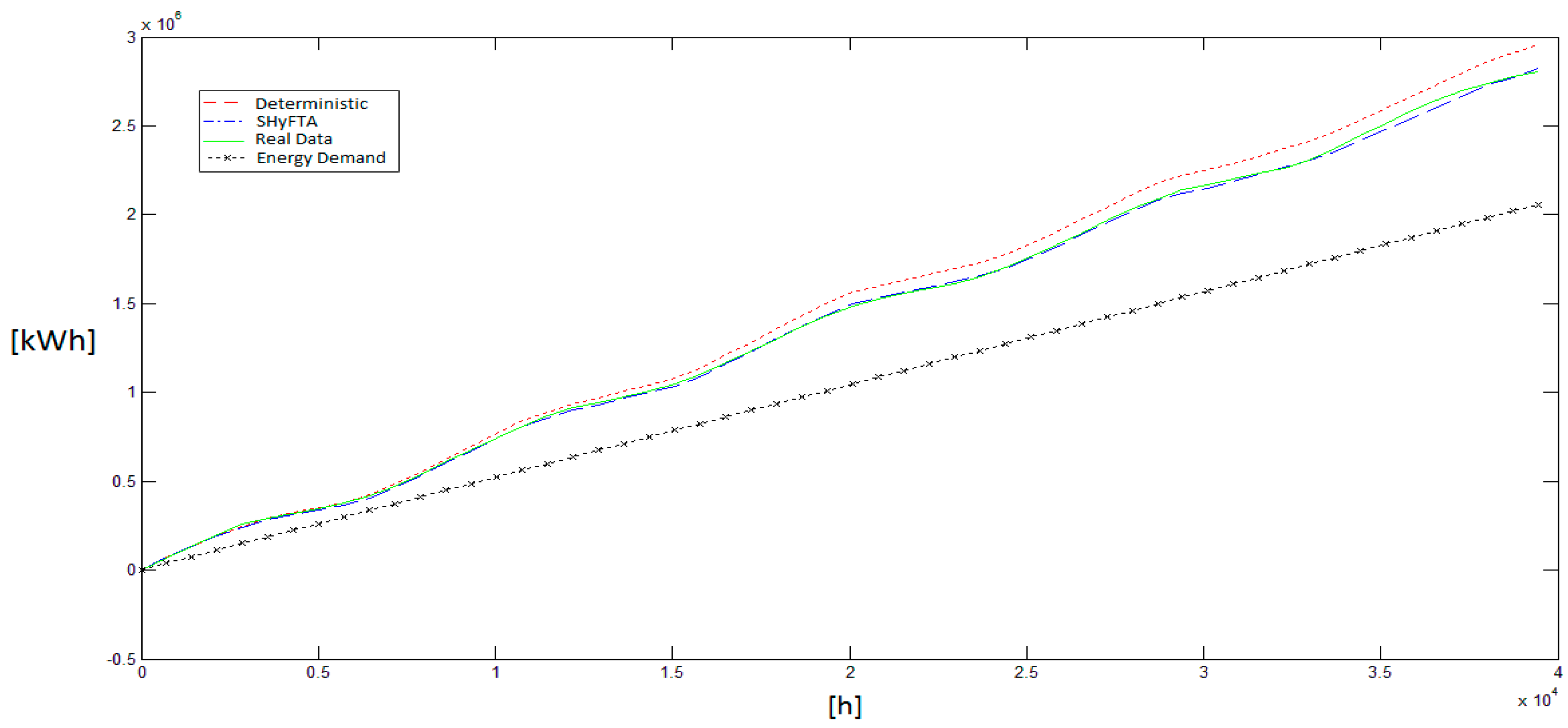
* corresponds with 40,173 h.

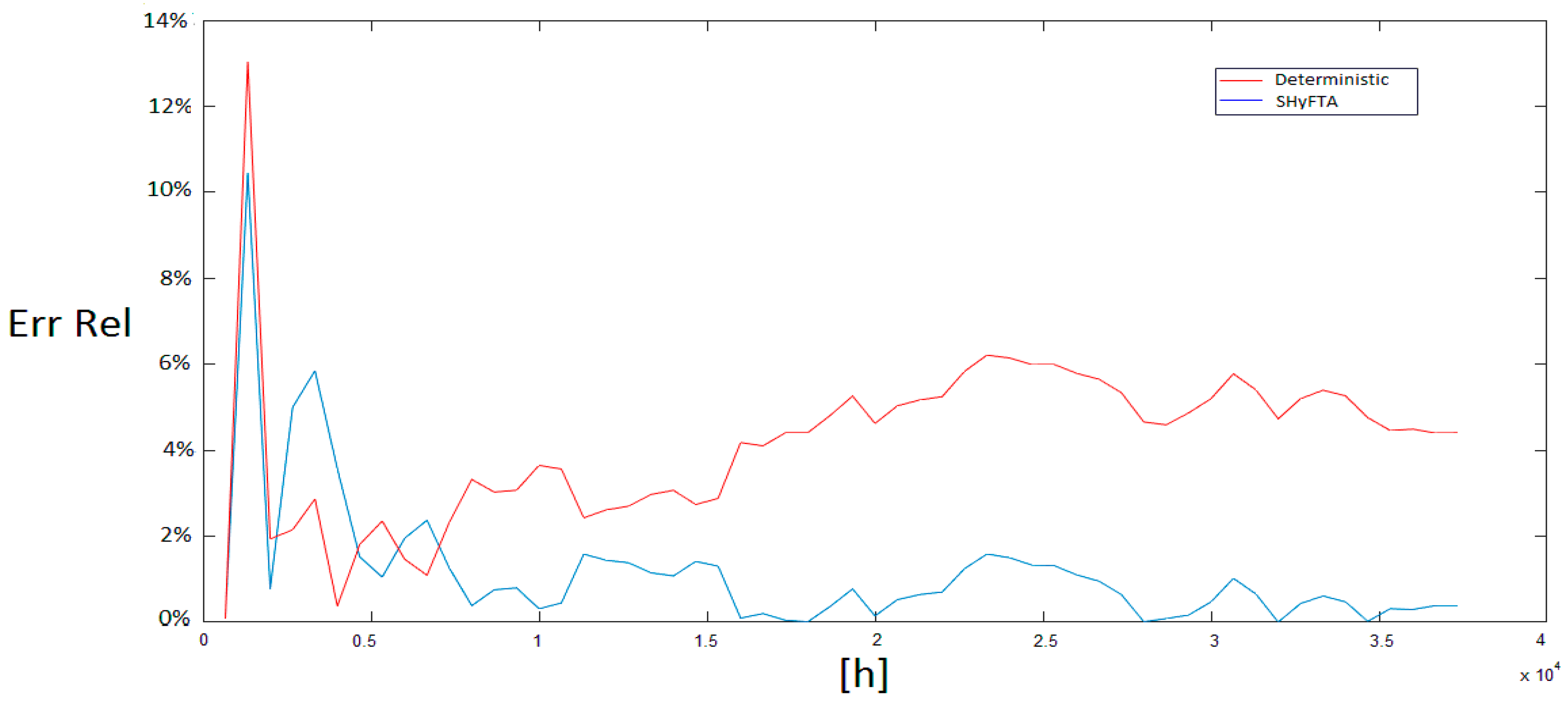
displays a comparison among the real data, the deterministic and the SHyFTA models in terms of energy produced and payback generated under the regime of IPER 2011. It is possible to notice that the results of the SHyFTA at the end of the observation period (see last row of Table 12 and Figure 13) matches with the real data aside the absolute error of the Monte Carlo simulation (±4681 kWh). We can observe that at the beginning of the simulation, the deterministic and the SHyFTA model are very close to the real data and the reason is that at the beginning of the power plant life there are no faults and performance degradation which affect the system. However, after a few months, the gap between the real data and the deterministic model starts to increase, whereas the difference with respect to the SHyFTA remains bounded to a maximum relative error of 2%, as shown in Figure 14 that plot the absolute relative error with respect to real data.

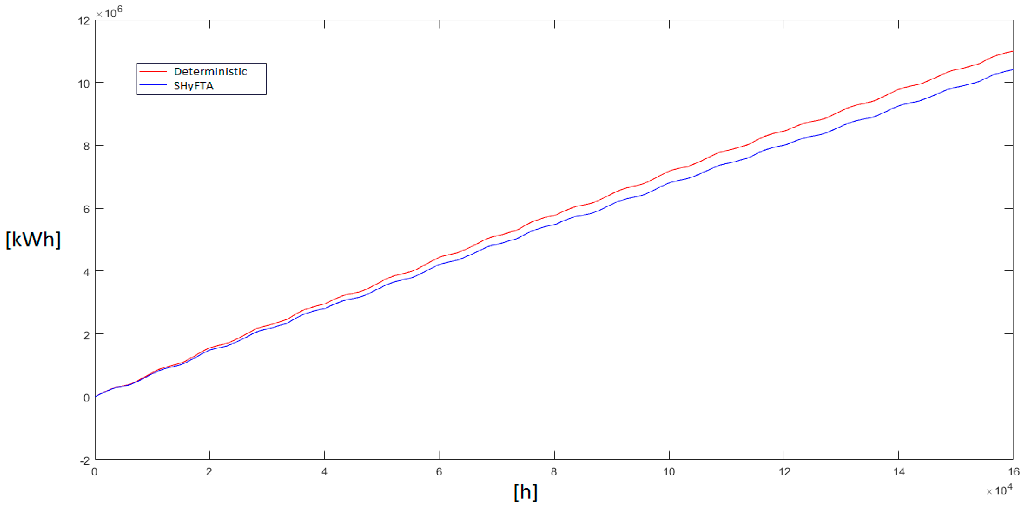
At this point, having tested the accuracy of the proposed method, it is possible to forecast the production of energy over 20 years of life in order to provide the owner of the plant with a more accurate estimation of production and economical revenues. To achieve this result, the simulation with the SHyFTA is extended to 20 years assuming that the physical input of the solar radiation and ambient temperature follow the same evolution described by the historical time series of the last 5 years. The Monte Carlo simulation has been set such to respect the same confidence level of the previous simulation. Under this setting, the absolute cumulative error of the time series sums up to 0.18%, that corresponds to ±20,480 kWh.

Figure 15 shows the results obtained and

Table 13. Comparison between the deterministic and the SHyFTA model throughout the remaining years of the plant life in terms of energy produced and positive payback generated under the regime of IPER 2011.

Year	Deterministic (kWh)	Payback (€)	SHyFTA (kWh)	Payback (€)
5	3,151,996	1,462,526	3,005,940 (±5166)	1,394,756 (±2375)
10	6,111,600	2,835,782	5,817,056 (±10,270)	2,699,114 (±4724)
15	8,955,165	4,155,197	8,516,286 (±15,352)	3,951,557 (±7062)
20	11,682,162	5,420,523	11,137,157 (±20,480)	5,167,641 (±9421)

allows a further comparison between the deterministic and the SHyFTA. In this case, it is possible to recognize at the end of the 20th year, a difference of about 545,000 kWh (±20,480 kWh) of loss of energy productivity. Under the regime of IPER 2011, at the end of the economic investment established at the 20th year from the start of the power plant, this lack of energy production corresponds to a cash short of about 250,000 € (±9421 €).

5. Conclusions

In this paper dynamic reliability is proposed as valuable paradigm for the modelling and the evaluation of renewable power plants. Dynamic reliability can address the limitations of traditional deterministic models, which are unable to account for the randomness of the primary resource and the concept of plant dependability.

Stochastic Hybrid Fault Tree Automaton (SHyFTA) has been presented as a valid modelling approach to evaluate the performance of renewable power plants. SHyFTA is able to model (i) the randomness of the primary resource; (ii) the performance deterioration; (iii) the faults and repair processes of the system components. Moreover, a SHyFTA model can be easily redesigned and simulated so as to assess the effect of alternative design decision on system performance.

In this paper, the main steps for the modeling of a SHyFTA have been defined and a case of study of real photovoltaic power plant was discussed. To demonstrate the accuracy of the results achieved with a SHyFTA simulation, the production of energy of the photovoltaic power plant has been estimated and compared with the deterministic model, exploiting as benchmark the data of production of the real photovoltaic power plant. Further comparisons between the SHyFTA and the deterministic model have been discussed also in terms of cash short, when estimating the expected productivity throughout the entire lifetime of the power plant (20 years). Further researches can exploit the potential of the SHyFTA model that can be easily modified to evaluate more appropriate design solutions which can include the use of trackers, or the integration with a system of batteries. More generally, it represents a valuable technique for the evaluation of other renewable technologies because the model of energy conversion can be always linked with the basic events of the fault tree model and can account, on the base of a statistic input, for randomness of productivity and system availability.

The SHyFTA analysis is based on Monte Carlo simulations, and therefore, the accuracy of the results and simulation times can require long computation time before to retrieve results with an acceptable precision. In conclusion, the main benefits of the proposed approach are twofold: on the one hand it allows to perform an estimation of the main process measures and on the other hand provides important information about the system health.