Nonlinear Disturbance Decoupling Control for Hydro-Turbine Governing System with Sloping Ceiling Tailrace Tunnel Based on Differential Geometry Theory

School of Hydropower and Information Engineering, Huazhong University of Science and Technology, Wuhan 430074, China
Energies 2018, 11(12), 3340; https://doi.org/10.3390/en11123340
Submission received: 12 November 2018
/
Revised: 25 November 2018
/
Accepted: 28 November 2018
/
Published: 30 November 2018
(This article belongs to the Section F: Electrical Engineering)
Abstract
:For hydropower stations with sloping ceiling tailrace tunnel (SCTT), the regulation quality of hydro-turbine governing system (HTGS) under the proportional-integral-derivative (PID) strategy is poor. In order to improve the regulation quality of HTGS, the nonlinear disturbance decoupling control (NDDC) based on differential geometry theory is firstly applied into the HTGS with SCTT. The rigorous and complete construction method of nominal output function is proposed. Based on the obtained nominal output function, a novel NDDC strategy for HTGS with SCTT is designed. The application and performance of NDDC strategy on HTGS with SCTT are revealed. The results indicate that the regulation quality of the HTGS with SCTT under NDDC strategy is obviously better than that under PID strategy. The NDDC strategy has a favorable applicability on SCTT. The robustness of the HTGS with SCTT under NDDC strategy is excellent. In real engineering cases, the NDDC strategy can be adopted to optimize the design of the governor and improve the power supply quality of hydropower station.
1. Introduction
Renewable energy is energy that is collected from renewable resources, which are naturally replenished on a human timescale, such as sunlight, wind, water, tides, waves, and geothermal heat. Renewable energy often provides energy in electricity generation. Today and in the near future, renewable energies are expected to be more widely implemented to help maintain sustainable growth and quality of life [1]. Sustainability must be achieved by using strategies that do not increase the overall carbon footprint. The water–energy nexus is crucial for quantifying the potential for energy recovery in any water system, and defining performance indicators to evaluate the potential level of energy savings is a key issue for sustainability [1]. Among all of the different types of renewable energy, the hydropower plant which utilizes the water energy stands out for its feasibility. Hydropower plays an important role as the main renewable source of energy generation with an installed capacity of 990 GW in 2012 worldwide contributing to climate protection [2]. Moreover, hydropower on a small scale, or micro-hydro, is one of the most cost-effective energy technologies to be considered for rural electrification in less developed countries [3].
The tailrace tunnel with a sloping ceiling is a new type of tailrace tunnel for the development of hydroelectric energy [4]. Nowadays, more and more hydropower stations with sloping ceiling tailrace tunnel (SCTT) have been designed and constructed. The role of hydropower stations with SCTT in the power supply side becomes more and more important.
The SCTT can reduce the length of pressurized tailrace tunnel. Then, the flow inertia of the pressurized tailrace tunnel becomes smaller. SCTT acts the role of surge tank to some extent. As a result, the water hammer pressure during the transient process can be effectively decreased and the unit becomes safer. Those are the advantages of the SCTT. Meanwhile, the setting of SCTT introduces the free water surface in the tailrace tunnel. Then different flow patterns would arise, which include pressurized flow, free flow, and pressurized-free mixed flow. Different flow patterns in SCTT make the transient processes of the hydropower station extremely complicated and present a huge challenge for the SCTT.
It is well known that the hydropower stations undertake the main work of peak regulation and frequency modulation in modern power systems. The regulation tasks of hydropower stations are realized by the hydro-turbine governing system (HTGS). For the hydropower station with SCTT, the HTGS is a nonlinear dynamic system [5]. For that complex layout of hydropower station, the general proportional-integral-derivative (PID) strategy, which is linear, cannot meet the requirements of high regulation quality. The regulation quality of HTGS is directly related to the power supply quality of hydropower station. In order to achieve a good power supply quality of hydropower station with SCTT, the design and application of advanced control strategies, especially the nonlinear control strategies, to the HTGS are necessary.
To the best knowledge of the author, the nonlinear control strategies have not been applied into the HTGS with SCTT. From the perspective of improving the regulation quality, it is necessary to study the nonlinear control of the HTGS with SCTT. Moreover, that study is also a meaningful attempt of nonlinear control technology for the regulation of HTGS, which can attract people’s attention on the issue of regulation quality and control for the HTGS with SCTT.
A novel nonlinear mathematical model of HTGS with SCTT is proposed in [5]. That model contains the dynamic equation of pipeline system which can accurately describe the motion characteristics of the interface of free surface–pressurized flow in SCTT. However, because of the complexity of the nonlinear model, it is difficult to analyze the regulation quality of the HTGS by conventional methods, such as phase plane method [6] and describing function method [7]. As a result, we cannot design advanced control strategies which are based on the analysis results of regulation quality. With the development of the theory of a nonlinear dynamic system and the theory of nonlinear system control, such as fuzzy control [8], bifurcation and chaos control [9,10], nonlinear decoupling control based on differential geometry theory [11,12], sliding mode control [13], artificial neural network control [14], particle swarm optimization algorithm [15], artificial sheep algorithm [16], fractional order PID control [17], nonlinear predictive control [18,19] and nonlinear H∞ control [20], and the improvement of the calculation and simulation capability of computer, now it is possible to study this special nonlinear dynamic system and design proper advanced control strategies. The nonlinear control methods in [8,9,10,11,12,13,14,15,16,17,18,19,20] are widely used in dynamic systems, such as mechanic and power systems. As an intelligent method, the fuzzy logic controller is widely used in industrial processes due to its inherent robustness [8]. The Hopf bifurcation relates to a type of relatively simple yet important dynamic bifurcation phenomena in nonlinear dynamic systems [9,10]. It is usually closely associated with the self-oscillation of dynamic system. The generalized generic model control within the framework of differential geometry can be easily applied on the processes possessing relative order larger than unity [11,12]. The sliding mode controller can be used for the compensation of the friction force acting within the control of a mechanical system [13]. Artificial neural networks are powerful tools for nonlinear statistical data modeling or decision making [14]. The particle swarm optimization algorithm has a nature of randomly searching, which enables them to approach the global optimum [15]. The artificial sheep algorithm is based on social behaviors of sheep flock and has been applied to the start-up process for pumped storage units [16]. The fractional order PID control is based on the fractional calculus theory and has been applied into some different fields in the past few years [17]. Nonlinear predictive control provides a flexible solution for the control of nonlinear multivariate plants under hard constraints [18,19]. The nonlinear H∞control theory has the capacity to cope with unknown disturbances [20].
In recent years, the nonlinear decoupling control method based on differential geometry theory has been introduced into the control of power systems [21,22,23,24,25,26]. Khalil et al. [21] introduced the basic concepts and principles of nonlinear decoupling control and differential geometry theory. Isidori [22] introduced the disturbance decoupling control and its application on nonlinear dynamic systems. Fang et al. [23] studied the nonlinear disturbance decoupling control for hydraulic turbogenerators regulating system and verifies that the dynamic performance of system can be improved. Akhrif et al. [24] investigated the application of a nonlinear controller to the multi-input multi-output model of a hydraulic turbine system and the proposed controller was based on a feedback linearization scheme. Gui et al. [25] studied the output regulation design method by means of nonlinear geometric control theory on the basis of the comprehensive nonlinear model. Anderson et al. [26] dealt with nonlinear optimization problems by using the linear quadratic method and obtained a good result. The accurate linearization using differential geometry theory has received widespread attention. Through proper transformation of nonlinear state and feedback, the nonlinear system can be globally and accurately linearized with respect to the state or input/output. Then the complicated nonlinear system can be transformed into a simple and completely controllable linear system. For the obtained linear system, the existing optimal control method, such as linear-quadratic optimal control theory, can be applied to design the control strategy for the original nonlinear system. That kind of accurate linearization method is different from the traditional approximate linearization method. No higher order nonlinear term is neglected during the linearization processes. Therefore, that linearization method is not only accurate but also of significance to the overall situation. For some special problems, such as the control of HTGS with SCTT, the corresponding nonlinear systems are non-minimum phase system [27,28]. If the differential geometry theory is directly applied to that kind of systems, the systems cannot be linearized globally. For the part that cannot be linearized, the zero dynamic stability is difficult to prove. That problem is usually called the zero-dynamic problem [25,29,30]. In order to avoid the zero-dynamic problem, predecessors always transform the original control system into minimum phase system by selecting a proper output function, and then linearize the obtained minimum phase system globally and accurately by differential geometry method [23,24,25]. However, the output functions are always constructed based on the predecessors’ experiences. The rigorous and complete construction method of the output function is not proposed. That problem becomes the biggest obstacle for the further popularization and development of the nonlinear decoupling control method. Overcoming that obstacle is one of the motivations of this paper.
In order to improve the regulation quality of the HTGS of hydropower station with SCTT, the nonlinear disturbance decoupling control (NDDC) based on differential geometry theory is firstly applied into the nonlinear HTGS with SCTT in this paper. That attempt is not carried out by the previous researchers. The novelty and innovation also contain the rigorous and complete construction method of the output function, the design method of NDDC strategy and the applicability of NDDC strategy on the SCTT.
This paper is organized as follows. First, in Section 2, the nonlinear mathematical model of HTGS with SCTT is presented. Then, in Section 3, the basic principle of the NDDC based on differential geometry theory is interpreted. In Section 4, the rigorous and complete construction method of the nominal output function is proposed. Based on the obtained nominal output function, the NDDC strategy is designed. The application and performance of the NDDC strategy on the HTGS with SCTT are revealed in Section 5. Finally, in Section 6, the whole paper is summarized and the conclusions are given.
2. Nonlinear Mathematical Model of HTGS
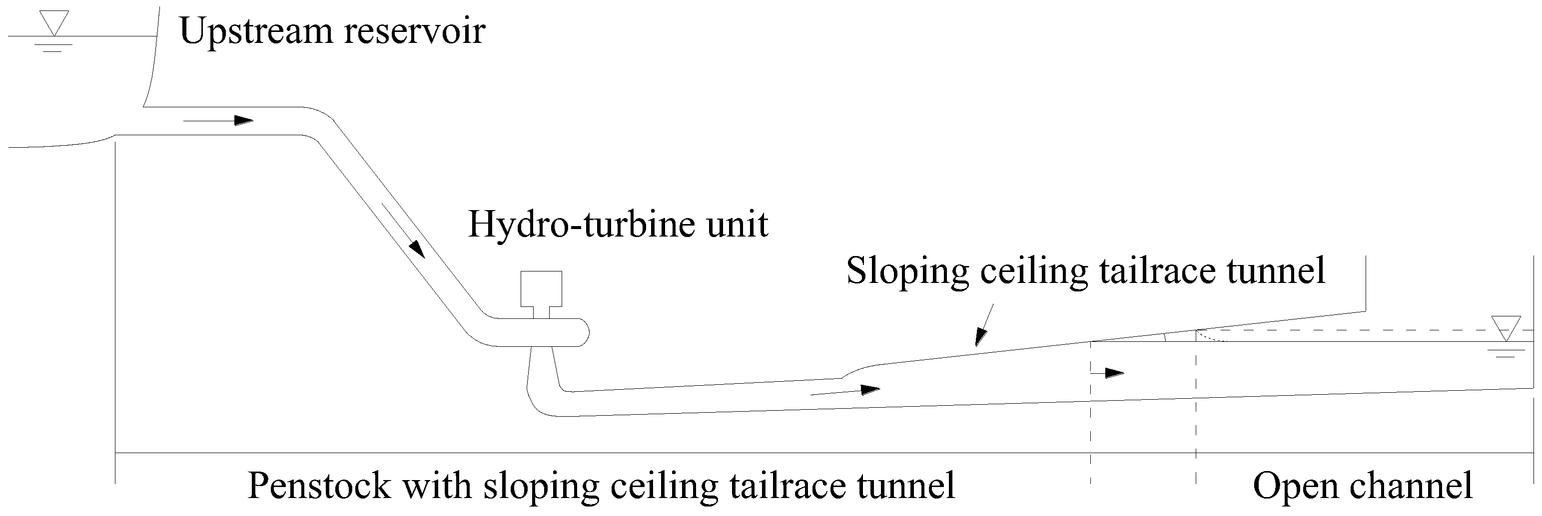
Figure 1 shows the pipeline and power generating system of the hydropower station with SCTT.
For the HTGS of hydropower station with SCTT, the basic equations and state equation are established in [5]. The HTGS with SCTT contains the following subsystems: penstock with sloping ceiling tailrace tunnel, hydro-turbine, generator, and governor. Under the external disturbance, the flow in the water diversion and the components of the power generating system enter the transient processes. During the process of mathematical modeling, the following assumptions are made:
- (1)
- The walls of penstock and the water in penstock are rigid. Thus, water hammer pressure caused by changes of the guide vane opening can be computed by using the rigid water-column theory.
- (2)
- The flow characteristics and moment characteristics of hydro-turbine are complex and nonlinear. It is difficult to directly express the nonlinear flow characteristics and moment characteristics. In this study, the changes of hydro-turbine speed, head and guide vane opening are small. Thus, the nonlinear relationships of hydro-turbine can be assumed as linear. Then the flow characteristics and moment characteristics can be analytically expressed, and the obtained expressions are convenient for theoretical analysis.
- (3)
- The dead band, backlash, and hysteresis are nonlinear components of governor. In this study, the dead band, backlash, and hysteresis are not in the regulating range of the governor. Therefore, we neglect the dead band, backlash and hysteresis. As a result, the regulating characteristics of the governor are not affected, and the model of the governor becomes linear and simpler.
- (4)
- The isolated operation condition is an important condition for the hydropower station. In this study, we aim to analyze the dynamic performance and control of HTGS under isolated operation condition, and the effect of power grid is not considered. Specifically, a single hydro-unit supplies power to an isolated load. The grid is regarded as a separate grid. The working condition of the hydropower station is the isolated operation, not the grid-connected operation. The generator is a synchronous generator. The first order generator equation is adopted.
The above assumptions are commonly used in the analysis of the dynamic performance and control of HTGS. The results obtained from the above assumptions are reasonable and can be directly applied to the practical engineering.
Reference [5] indicates that the HTGS with SCTT is a nonlinear dynamic system. The nonlinear mathematical model of HTGS contains the following basic equations: dynamic equation of penstock with SCTT, moment equation, and discharge equation of hydro-turbine, first derivative differential equation of generator and equation of governor [5]. Under load disturbance mg, the state equation of the nonlinear dynamic system without control can be obtained by combining the basic equations and the result is as follows [5]
The nomenclatures in Equation (1) are presented in Table 1. Equation (1) represents the dynamic characteristics of the HTGS with SCTT. The state equation includes the characteristic parameters and state variables of the nonlinear system. Specifically, q, x and y are the three state variables of the HTGS. Therefore, the HTGS with SCTT is a third order dynamic system. In Equation (1), the only nonlinear term comes from , which is caused by the free surface-pressurized flow in SCTT. For the system of Equation (1), the disturbance variable, i.e., the input signal, is the load disturbance mg. The output signal is selected as x because the regulation quality of the HTGS is mainly evaluated by the dynamic performance of x. The control strategy of governing system is described by u which will be designed in the following sections.
Note that:
- (1)
- h = (H − H0)/H0, q = (Q − Q0)/Q0, x = (N − N0)/N0, y = (Y − Y0)/Y0 and mg = (Mg − Mg0)/Mg0 are the relative deviations of corresponding variables. The subscript ‘0’ refers to the initial value.
- (2)
- , , , .
- (3)
- The transfer coefficients of turbine are defined as follows: , , , , and . The transfer coefficients come from the linearized model of the turbine and are used to describe the moment and discharge characteristics of turbine. They reflect the effect of the change of turbine efficiency on the turbine operation. The values of transfer coefficients are related with the structure parameters and operating point of the turbine. In practical applications, the transfer coefficients can be calculated according to their definition and the model comprehensive characteristics curves of turbine.
For a n-dimensional single-input single-output affine nonlinear system, the model is in general written as
where is the state vector; and are both n-dimensional vector fields; u is the regulator output of governor, in the meantime, it is the input variable of the following mechanism; is the scalar nominal output function, specifically, it is the function of state vector . For the system, there is a disturbance. The type of the disturbance mainly depends on the system characteristics, operating conditions, and research purpose. For the nonlinear system (1), the regulation quality under load adjustment is the research purpose. Therefore, mg is selected as the disturbance.
The nonlinear system (1) can be transformed into the form described by Equation (2), and the expressions of , and are presented in Appendix A. For the HTGS with SCTT studied in this paper, the input signal is mg and the output signal is x. The control strategy of governing system is described by u. is the function of q, x and y, in which q, x, and y are the state variables of the HTGS. It should be noted that: in the practical engineering projects, the dynamic performances of q and y are not important for the power supply quality. Hence, based on the research purpose of this paper, the dynamic performances of q and y will not be analyzed in the following parts. The state characteristics of the nonlinear system are described by and . , and contain the characteristic parameters of the nonlinear system (1), i.e., tanα, λ, Tws, hf, hydro-turbine transfer coefficients (i.e., eh, ex, ey, eqh, eqx and eqy), Ta, Ty and eg. The above characteristic parameters have obviously effects on the regulation quality of the HTGS. The determinations of the characteristic parameters are the key aspect of the design of the HTGS with SCTT. In the process of the design, the characteristic parameters should be selected and optimized. For a built hydropower station under an operating condition, the characteristic parameters are known.
3. Basic Principle of the NDDC Based on Differential Geometry Theory
The linearization of nonlinear system by coordinate transformation is the essence of differential geometry method. Compared with the traditional linearization methods of nonlinear system, which are approximate, the linearization through differential geometry method is accurate because no higher order nonlinear term is omitted. Moreover, that kind of linearization is a global linearization, and it is applicable in the whole region where the coordinate transformation is valid [11,12,21,22].
For the nonlinear system (2), the necessary and sufficient condition for the decoupling of the output with respect to the disturbance is as follows: the system relative degree equals the order of the system [23,25]. Then, a coordinate transformation can be chosen to transform the nonlinear system (2) into a linear system globally and accurately. The chosen coordinate mapping is
where is the i-order Lie derivative of the nominal output function with respect to the vector field , and .
After the coordinate transformation using Equation (3), the nonlinear system (2) is transformed into the following canonical form in the new coordinate system
where , . is the linear control strategy of the linear canonical form (4), and it is obtained from the coordinate transformation and expressed as [23,25].
According to Equation (3), the decoupling of output with respect to the disturbance can be carried out. Then the disturbance decoupling control strategy of nonlinear system (2) is obtained as
The optimal control strategy for is denoted as . The determination of is presented in Appendix B. Substituting into Equation (5) yields the NDDC strategy for HTGS with SCTT based on differential geometry theory under the linear-quadratic optimal control.
4. Design of the NDDC Strategy for HTGS
Control objective: If the hydro-turbine unit goes through an external load disturbance during normal operation under frequency regulation mode, the whole hydropower station enters the transient process. During that process, the unit frequency deviates from the initial value (i.e., rated frequency, 50 Hz), and the HTGS begins to regulate the unsteady status. For the regulation of the HTGS, the guide vane opening is used as the controlled variable and the relative deviation of frequency is used as the control basis. The control objective is to make the unit frequency return to the initial value rapidly and smoothly. Then the high quality power supply can be achieved. As for the nonlinear system (1), the equilibrium point of the relative deviation of frequency should be 0 based on the control objective. Combining and yields the unique equilibrium point of system (1)
4.1. Construction of the Nominal Output Function
When we carry out the coordinate transformation for the original nonlinear system, the selection of the nominal output function mainly determines the form of the state equation of the new linear system. Moreover, the dynamic and static characteristics of the new controlled system are directly affected by the nominal output function. Hence, the selection of the nominal output function is the key of the NDDC. The selected nominal output function must meet the following two requirements simultaneously:
- Satisfying the control objective of the original nonlinear system, i.e., the equilibrium point of system is expressed by Equation (6).
- Satisfying the necessary and sufficient condition for the decoupling of the output with respect to the disturbance, i.e., the system relative degree equals to the order of the system. As a result, the HTGS is a minimum phase system with respect to the selected output. Note that: if the output function is selected as the output signal x, the HTGS becomes a non-minimum phase system. Then the system can be linearized globally and accurately by differential geometry method. For the original nonlinear system (1), the system relative degree should be 3. Therefore, the corresponding nominal output function must satisfy
Equation (7) indicates that the 1-order Lie derivatives of and with respect to are both equal to 0, while the 1-order Lie derivative of with respect to is not equal to 0, where and are the 1-order Lie derivative and 2-order Lie derivative of with respect to .
Based on the requirements (i) and (ii), a step-by-step procedure for the construction of nominal output function is proposed and clarified in the following paragraphs. Note that a detailed derivation and explanation of the Step 1, Step 2, and Step 3 is presented in Appendix C.
Let the form of the nominal output function be
where , , are the functions of q, x, y, respectively, and they do not contain constant terms. C is the undetermined constant.
Step 1:
Using and the expression of the nominal output function, i.e., Equation (8), we can obtain
Step 2:
Based on , Equation (9) and the expression of , we can obtain the nominal output function as
Step 3: Equilibrium point
According to the basic principle described in Section 3, the NDDC strategy for the nonlinear system (1) based on differential geometry theory under the linear-quadratic optimal control is expressed as
Then based on , Equation (6), Equation (10), equilibrium point and the expressions of , , , and , we can obtain the complete expression of the nominal output function as
From Equation (12), it is easy to obtain and the following results:
which indicates that the nominal output function Equation (12) constructed by the above procedure meets the requirements (i) and (ii). For the nonlinear system (1) that applies the nominal output function Equation (12), the output can be decoupled with respect to the disturbance, and the nonlinear system can be linearized globally and accurately.
4.2. Design of the NDDC Strategy
Using Equation (12), we can obtain the expressions of , , and , which are presented in Appendix D. Then by combining , , and Equation (A3) yields .
By substituting the expressions of , , , , , and into Equation (11), we obtain the complete expression of the NDDC strategy based on differential geometry theory under the linear-quadratic optimal control. Replacing in the nonlinear system (1) by , we achieve the NDDC for HTGS with SCTT.
It should be noted that the above construction method of the nominal output function and design method of the NDDC strategy can be extended to fourth order and higher order nonlinear dynamic systems. To better understand the extension of the proposed construction method in this paper, the example for a fourth order nonlinear dynamic system is given as follows:
The state vector for the fourth order nonlinear dynamic system is denoted by . The form of the nominal output function is selected as , where , , and are the functions of , , and , respectively, and they do not contain constant term.
For the fourth order nonlinear dynamic system, the requirements (i) and (ii) are written as:
- (i).
- Satisfying the control objective of the original nonlinear system.
- (ii).
- The corresponding nominal output function must satisfy
By a four-step procedure, i.e., Step 1: , Step 2: , Step 3: , and Step 4: Equilibrium point , we can get the expression of the nominal output function . Then the correctness of the obtained can be verified by . Finally, based on the obtained , we achieve the NDDC for fourth order nonlinear dynamic system by the same method and procedure used in Section 4.2.
5. Numerical Example
Based on numerical simulations of a project example, this section illustrates the application and performance of the NDDC strategy to the HTGS with SCTT. Firstly, the comparison of regulation quality between the NDDC strategy and PID strategy is carried out. Then, the applicability of the NDDC strategy on the SCTT is presented. Finally, the robustness of the HTGS under NDDC strategy is analyzed.
A hydropower station with SCTT is taken as example. The basic data of the hydropower station are: rated head H0 = 70.7 m, rated discharge Q0 = 466.7 m3/s, Ta = 8.77 s, B = 10.0 m, Tws = 3.20 s, hf = 2.68 m, Hx = 23 m, tanα = 0.03, λ = 3, eg = 0, Ty = 0.2 s, and g = 9.81 m/s2. eh = 1.453, ex = −0.900, ey = 0.415, eqh = 0.565, eqx = −0.132, and eqy = 0.682. A step load disturbance of mg = −0.1 is selected as the operating condition.
5.1. Regulation Quality of the HTGS Using the NDDC Strategy
The NDDC strategy for the HTGS with SCTT has been designed in Section 4.2. In this section, the comparison of regulation quality between the NDDC strategy and PID strategy is presented to illustrate the performance of NDDC strategy on the HTGS.
For the PID strategy, the control equation of the governor is [31]
where , , and are proportional gain, integral gain, and differential gain, respectively.
Combining the Equation (1) and Equation (13) yields the HTGS with SCTT under PID control. The gains for the optimal regulation quality of HTGS with PID controller are determined by the Stein formula [32]
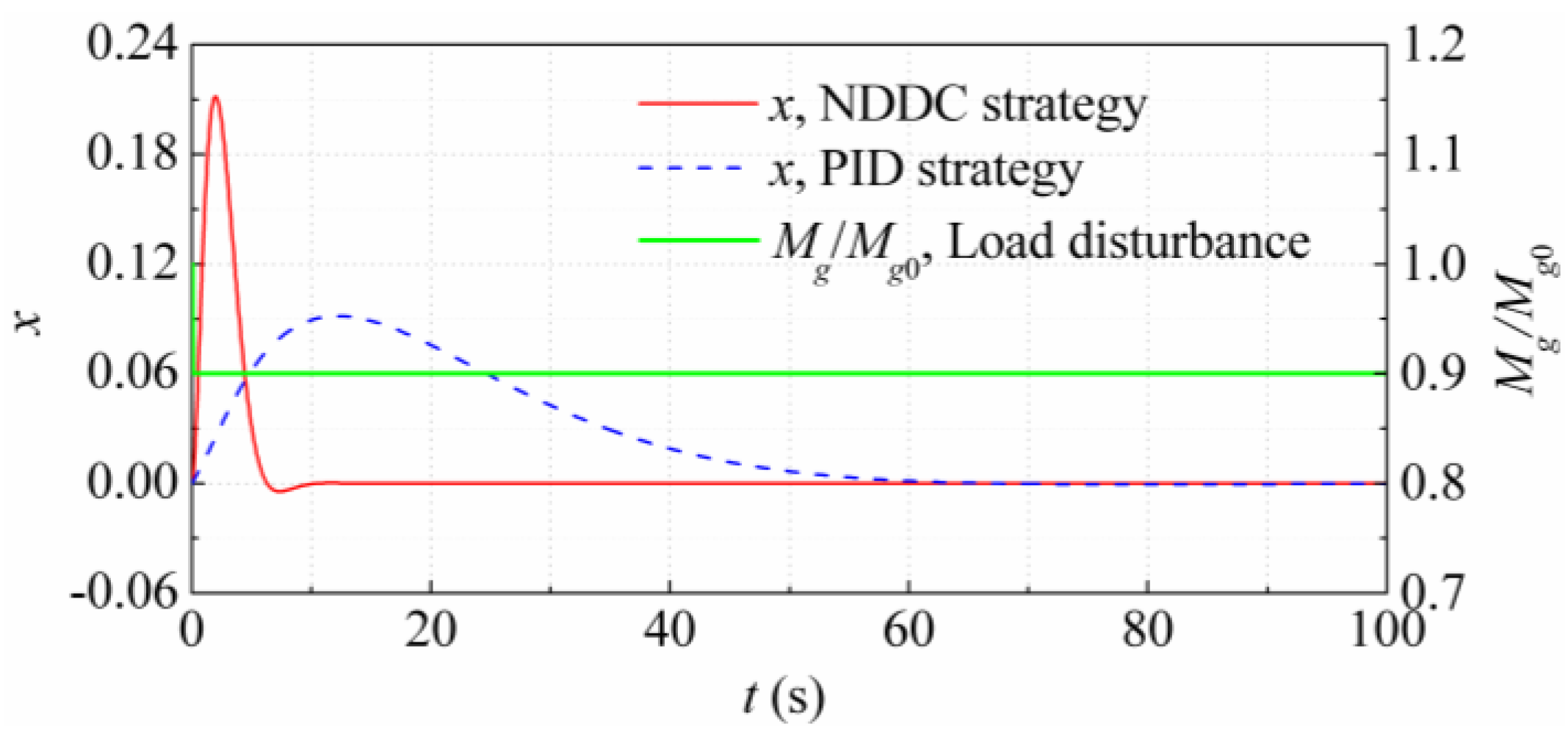
Using Equation (14), we can obtain the optimal combination of PID gains as Kp = 1.827, Ki = 0.190 s−1 and Kd = 2.923 s. Then, Figure 2 shows the dynamic response processes of x using the NDDC strategy under the linear–quadratic optimal control and using the PID strategy under the Stein formula. In Figure 2, the load disturbance is set at an anticlimax of rated power output from 100% to 90% at t = 0 s.
Figure 2 shows that, under the NDDC strategy, the HTGS with SCTT is rapid and sensitive. The unit frequency can return to the initial value (i.e., rated frequency) in 10 s. Under the PID strategy, it takes 70 s for the unit frequency to return to the initial value. The results indicate that the regulation quality and the response speed under the NDDC strategy are obviously better than those under the PID strategy. That is because linear controllers are inadequate even for controlling the moderately nonlinear processes. The HTGS with SCTT is a complicated nonlinear system. As a linear controller, the PID strategy is inadequate for the regulation of HTGS with SCTT. Conversely, the NDDC strategy is a nonlinear controller and is specially designed for HTGS with SCTT. Therefore, the NDDC strategy is adequate for the regulation of HTGS with SCTT.
After the disturbance, the initial peak of the dynamic response process of x under NDDC strategy is high. It is clear that a high pressure on the guide vane would be caused during the fast change of x, but we have to point out that the high pressure is still safe for the guide vane. The reason is that the peak of x is only about 0.2. In the practical engineering, it is always required that the peak of x does not exceed about 0.5, accordingly, the pressure on the guide vane does not exceed the standard. Moreover, the dangerous condition for the pressure on the guide vane usually appears in the load rejection process. The operating condition studied in this paper is load adjustment. The amplitude of load variation is small, and the absolute value of mg is usually less than 0.1. Therefore, under the NDDC strategy, the pressure on the guide vane is safe.
5.2. Applicability of the NDDC Strategy on the SCTT
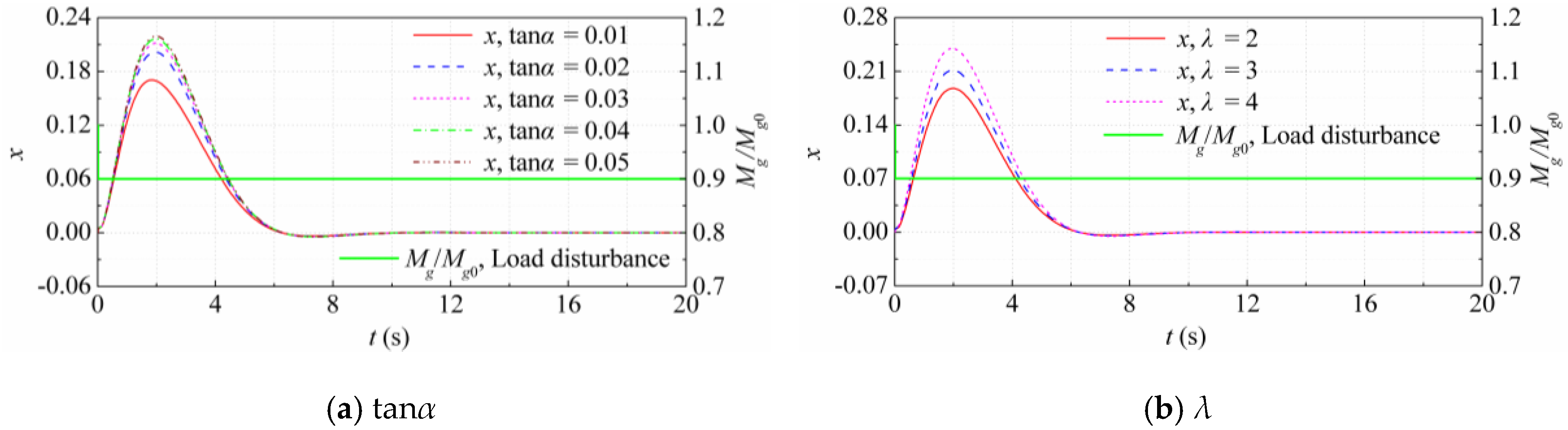
For the SCTT, tanα and λ are the two most significant parameters of the shape design [4,5]. tanα describes the ceiling slope, and λ represents the section form. As for the NDDC strategy, the applicability on the SCTT and the control performance on the regulation quality of HTGS mainly depend on the applicability of the strategy on the two parameters. tanα usually values from 1% to 5%. 2, 3, and 4 of λ represent the rectangle, arch, and roundness sectional forms, respectively. When tanα or λ takes different values, the dynamic response processes of x under the NDDC strategy are shown in Figure 3. Note that the default values of the variables are as follows: tanα = 0.03, λ = 3 and mg = −0.1.
Figure 3 shows that:
- (1)
- For tanα, with the increase of tanα, the peak value of the unit frequency becomes larger and larger while the increasing amplitude becomes lower. Under different tanα, the time that the unit frequency takes to return to the rated frequency is almost the same. For λ, when λ increases, the peak value of the unit frequency becomes larger and larger and the increasing amplitude is very close. Under different λ, the time that the unit frequency takes to return to the rated frequency is almost the same.
- (2)
- The NDDC strategy has a favorable applicability on the HTGS with SCTT. When the two most significant parameters of the shape design change and excellent performance of regulation quality can be guaranteed and achieved by the HTGS, and the dynamic response of x can always return to the rated frequency rapidly and smoothly. The results shown in Figure 3 have a specific guidance function for the shape design of the SCTT. Under the NDDC strategy, the regulation quality of the system becomes better with the decrease of tanα and λ. Hence, from the perspective of improving the regulation quality of the system, tanα and λ should take small values during the shape design. By considering different factors comprehensively—including regulation quality, stability, construction investment, construction difficulty, and construction period—we can finally determine the optimal shape parameters of the SCTT.
- (3)
- For the HTGS with SCTT, the only nonlinear term comes from , which is caused by the free surface-pressurized flow in SCTT. The NDDC strategy is specially designed for HTGS with SCTT to regulate the nonlinear element. Therefore, from the perspective of physical essence of the problem, the NDDC strategy always has a favorable applicability on the SCTT, including the parameters tanα and λ.
5.3. Robustness of HTGS Using the NDDC Strategy
Robustness is a significant performance index of control system. In order to test the robustness of the HTGS with SCTT using NDDC strategy, the robustness analysis is carried out based on the effect analysis of characteristic parameters on the dynamic response of x. Both qualitative and quantitative results of the robustness analysis are given. Specifically, the qualitative results mean the visual variation laws of the dynamic response processes of x when the characteristic parameters change. The quantitative results mean the qualitative performance index for assessing the robustness features. The qualitative performance index selected in this paper, i.e., robustness index (RI) [33,34,35,36,37], is presented in Appendix E.
For the HTGS with SCTT studied in this paper, the design variables are the state variables of the HTGS, i.e., . The design parameters contain Tws, hf, hydro-turbine transfer coefficients (eh, ex, ey, eqh, eqx, and eqy), Ta, Ty, eg, mg, tanα, and λ. The performance functions are the functions of the state variables and design parameters that at the right side of the equal signs in the system (1). Because of the extremely complex expressions of the HTGS (1) and the NDDC strategy, which are presented in Section 2 and Section 4, respectively, the calculation results of the RI will be given directly. The computational method is based on the above definitions and the extremely complex intermediate processes are not shown in the following parts.
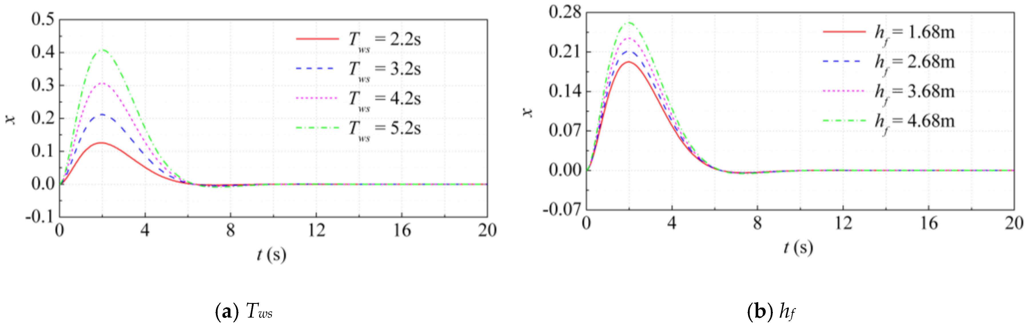
For the robustness analysis of the HTGS with SCTT under NDDC strategy, the characteristic parameters include four aspects: hydraulic parameters, mechanical parameters, electrical parameters, and disturbance. Specifically, Tws and hf are selected as the hydraulic parameters, and the results are shown in Figure 4 and Table 2. Hydro-turbine transfer coefficients (i.e., eh, ex, ey, eqh, eqx, and eqy), Ta and Ty are selected as the mechanical parameters, and eg is selected as the electrical parameter. The results are shown in Figure 5 and Table 2. mg is selected as the disturbance and the result is shown in Figure 6 and Table 2. In order to fully reflect the robustness of the HTGS under NDDC strategy, the calculation results of the RI corresponding to Figure 2 and Figure 3 are also given in Table 2. Moreover, under the PID strategy, the value of RI of the HTGS at Stein point is 2.306.
Note that the default values of some variables are as follows: Tws = 3.2 s, hf = 2.68 m; The actual hydro-turbine transfer coefficients are: eh = 1.453, ex = −0.900, ey = 0.415, eqh = 0.565, eqx = −0.132 and eqy = 0.682; Ta = 8.77 s, Ty = 0.2 s, eg = 0; mg = −0.1; tanα = 0.03, λ = 3. All the changes of selected parameters are in normal variation ranges. The ideal hydro-turbine transfer coefficients are: eh = 1.5, ex = −1, ey = 1, eqh = 0.5, eqx = 0, and eqy = 1.
Figure 4 shows that, with the increase of Tws and hf, the peak value of the unit frequency becomes larger and larger and the increasing amplitude is homogeneous. Under different Tws or hf, there is still only one oscillation and the time that the unit frequency takes to return to the rated frequency is almost the same. The comparison between Figure 4a,b shows that the effect of Tws on the dynamic response process of x under the NDDC strategy is more obvious that that of hf. The dynamic response process of x under the NDDC strategy is more sensitive with respect to the change of Tws.
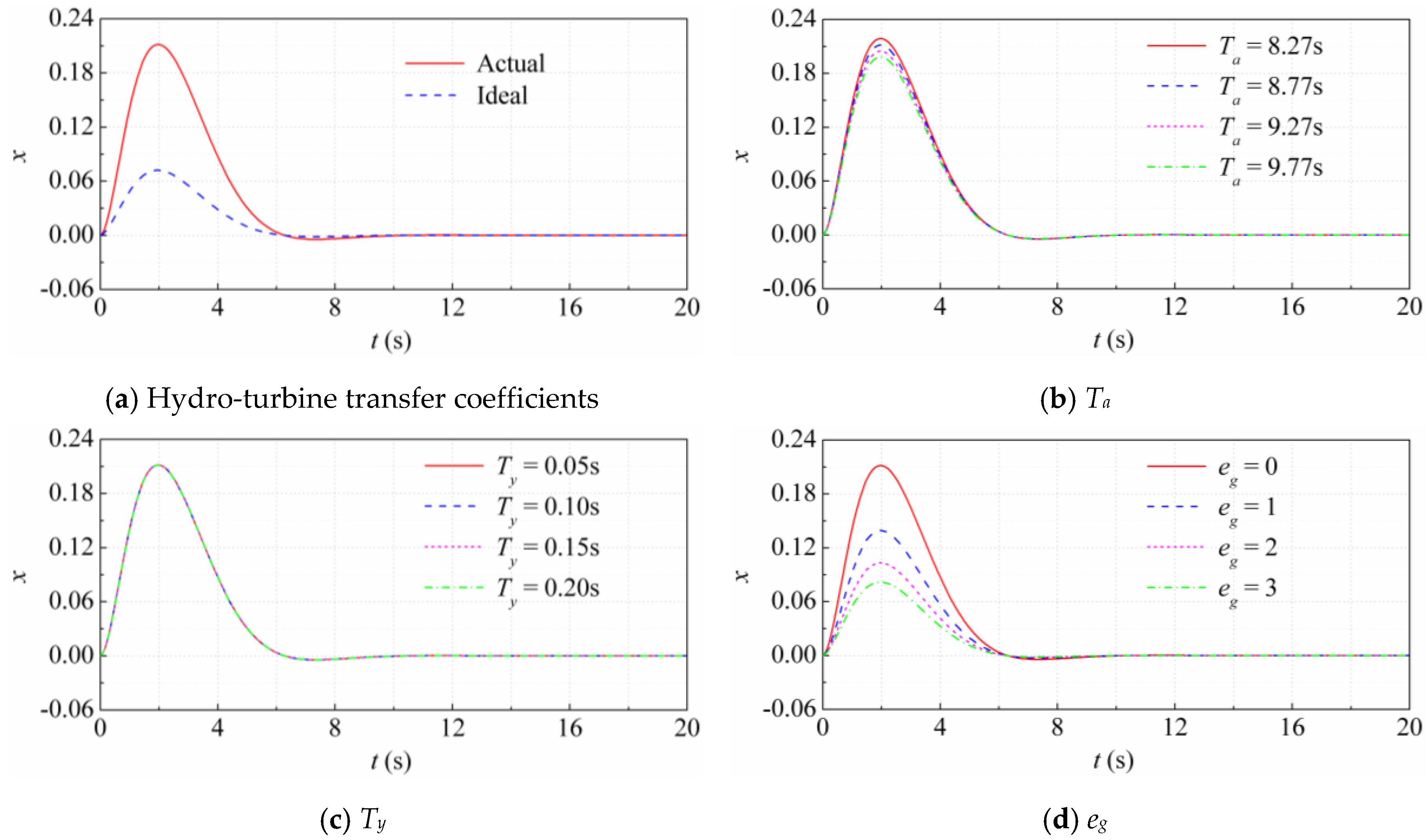
Figure 5 shows that:
- (1)
- The hydro-turbine transfer coefficients have an obvious effect on the dynamic response processes of x under the NDDC strategy. When the hydro-turbine transfer coefficients change from ideal values to actual values, the peak value of the unit frequency becomes larger. Under different hydro-turbine transfer coefficients, there is still only one oscillation and the time that the unit frequency takes to return to the rated frequency is almost the same.
- (2)
- Ta only has a slight effect on the dynamic response process of x under the NDDC strategy. With the decrease of Ta, the peak value of the unit frequency becomes larger and larger while the increasing amplitude becomes greater. Under different Ta, there is still only one oscillation and the time that the unit frequency takes to return to the rated frequency is almost the same.
- (3)
- Ty almost has no effect on the dynamic response process of x under the NDDC strategy. With the change of Ty, the dynamic response process and peak value of the unit frequency keep the same. Under different Ty, there is still only one oscillation and the time that the unit frequency takes to return to the rated frequency is the same.
- (4)
- eg has an obvious effect on the dynamic response processes of x under the NDDC strategy. With the decrease of eg, the peak value of the unit frequency becomes larger and larger while the increasing amplitude becomes greater. Under different eg, there is still only one oscillation and the time that the unit frequency takes to return to the rated frequency is almost the same.
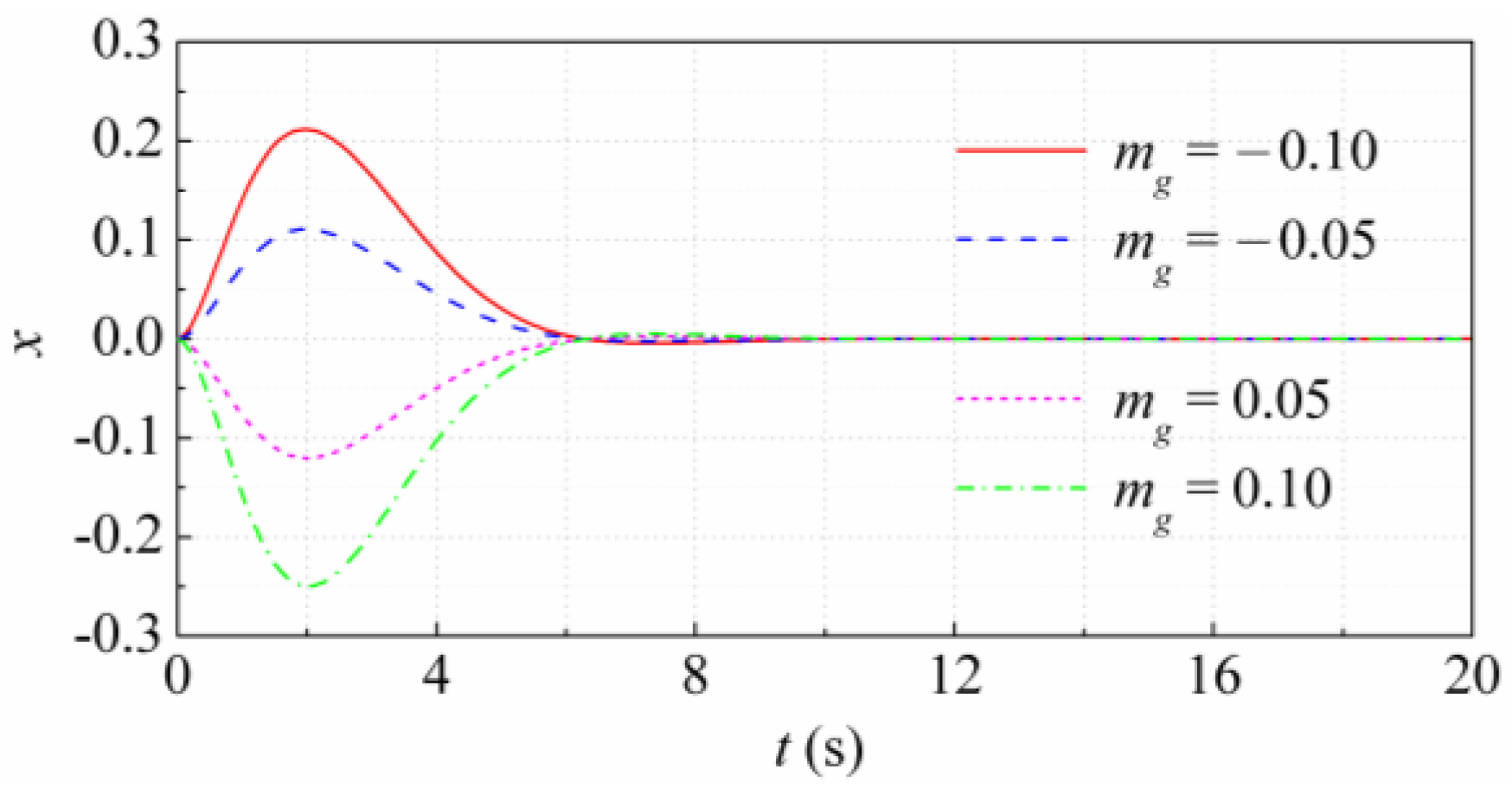
Figure 6 shows that mg has an obvious effect on the dynamic response processes of x under the NDDC strategy. When mg is less than zero, the peak value of the unit frequency is greater than zero. When mg is greater than zero, the peak value of the unit frequency is less than zero. With the increase of the absolute value of mg, the peak value of the unit frequency becomes larger. Under different mg, there is still only one oscillation and the time that the unit frequency takes to return to the rated frequency is almost the same.
Table 2 shows that:
- (1)
- Under the NDDC strategy, the values of RI of the HTGS at different parameters and values are between 1 and 2. Tws, hydro-turbine transfer coefficients, eg, and tanα have an obvious effect on the value of RI. hf, Ta, mg, and λ has a slight effect on the value of RI. Ty almost has no effect on the value of RI. The above results are consistent with those in Figure 4, Figure 5 and Figure 6, which indicates that the quantitative index RI can accurately reflect the robustness of HTGS. Moreover, the quantitative index RI is much easier for the analysis and comparison of robustness.
- (2)
- Essentially, the effects of different parameters and values on RI depend on their importance degree in the HTGS. For the regulation of HTGS, the effects of Tws, hydro-turbine transfer coefficients, eg and tanα are primary, while the effects of hf, Ta, mg, and λ are secondary. Moreover, Ty almost has no effect on the stability and regulation quality of HTGS.
- (3)
- Under the PID strategy, the value of RI of the HTGS at Stein point is 2.306, which is greater that under the NDDC strategy. It is well known that the Stein point is the optimal combination of PID gains for the dynamic response process of system. Then we can judge that the robustness of the HTGS using the NDDC strategy is better than that using the PID strategy.
By combining the results of Figure 4, Figure 5 and Figure 6 and Table 2, we can get that the robustness of the HTGS using the NDDC strategy is excellent. The RI of the HTGS using the NDDC strategy is less than that using the PID strategy, which indicates that the robustness of the former is better than that of the latter. Moreover, under different characteristic parameters and disturbance values, the RI of the HTGS using the NDDC strategy keeps small, which indicates that the system has a strong anti-interference ability. When the characteristic parameters change, the regulation quality and the response speed of the governing system are less affected. For the dynamic response processes of x, the number of oscillations always remains the same. The unit frequency can return to the rated frequency rapidly and smoothly, and the required time is very close.
Compared with the PID strategy, the structure of the NDDC strategy is more complicated. Therefore, the design of the NDDC controller is more difficult than that of the PID controller. However, in modern control system and technique, the structure design of the controller is not an obstacle. Moreover, the structure design of the controller is the job of the governor manufacturer and is one-time investment. The user, i.e., the hydropower station, is not affected by that issue. Conversely, for the hydropower station, the NDDC strategy is easier to use than the PID strategy. The reason is that is the NDDC strategy itself is a kind of optimal control. When the structure of the NDDC strategy is designed, the regulation quality of HTGS is optimal. However, the regulation quality of HTGS under the PID strategy depends on the values of , , and , which are difficult to determine the optimal combination. When the PID strategy is applied, too much work is needed to select the optimal combination of , , and . The most important as well as the last aspect is that the regulation quality of HTGS under the NDDC strategy is obviously better than that under the PID strategy. The regulation quality of HTGS is directly related with the power supply quality of hydropower station, and the power supply quality is one of the topics people pay the most attention. In a word, compared with the PID strategy, the NDDC strategy has obvious advantages and is worthy of spreading to application.
6. Conclusions
In order to improve the regulation quality of HTGS of hydropower station with SCTT, the NDDC based on differential geometry theory is firstly applied into the nonlinear HTGS with SCTT in this paper. That attempt is not carried out by the previous researchers. The novelty also contains the rigorous and complete construction method of the output function, the design method of NDDC strategy, and the applicability of NDDC strategy on the SCTT.
Firstly, the nonlinear mathematical model of HTGS with SCTT is presented. Then, the rigorous and complete construction method of the nominal output function is proposed. Based on the obtained nominal output function, the NDDC strategy is designed. Finally, the application and performance of the NDDC strategy on the HTGS with SCTT are revealed. The major conclusions are summarized as follows:
- (1)
- The construction of the nominal output function is the key of the design of the NDDC strategy based on differential geometry theory. The rigorous and complete construction method of the nominal output function is determined by the control objective of the original nonlinear system and the necessary and sufficient condition for the decoupling of the output with respect to the disturbance. Based on the obtained nominal output function, the complete expression of the NDDC strategy based on differential geometry theory under the linear-quadratic optimal control is obtained by coordinate transformation.
- (2)
- Under the NDDC strategy, the HTGS with SCTT is rapid and sensitive. The unit frequency can return to the initial value (i.e., rated frequency) in 10 s. The regulation quality and response speed under the NDDC strategy are obviously better than those under the PID strategy. The NDDC strategy has a favorable applicability on the HTGS with SCTT. When the two most significant parameters (i.e., tanα and λ) of the shape design change, excellent performance of regulation quality can be guaranteed and achieved by the HTGS, and the dynamic response of x can always return to the rated frequency rapidly and smoothly. From the perspective of improving the regulation quality of the system, tanα and λ should take small values during the shape design under the NDDC strategy. The robustness of the HTGS using the NDDC strategy is excellent, and the system has a strong anti-interference ability.
The applications of the NDDC strategy in real case include, but not limited to:
- (1)
- The NDDC strategy can be applied to the design of the controller for the HTGS with SCTT. The obtained controller using NDDC strategy can improve the regulation quality compared with the PID controller.
- (2)
- The NDDC strategy can be applied to the optimization of the design parameters of SCTT. For the HTGS with SCTT under NDDC strategy, the design parameters of SCTT can be determined based on the analysis results in Section 5 to obtain good regulation quality.
Funding
This research received no external funding.
Conflicts of Interest
The author declares no conflict of interest.
Appendix A
Appendix B
For the canonical form (4), the requirements for the system performance and control energy can be described by the following quadratic performance index
where and are symmetrical positive definite weight matrixes. The purpose of the optimal control is to find the suitable and , and then design the linear control strategy to minimize .
If the control strategy is selected as a state feedback control, the optimal control strategy that can minimize has the following form, i.e., [26]
where is the optimal gain vector. If the weight matrixes and are selected as the identity matrixes, i.e., and , which is a common practice in the linear-quadratic optimal control [23,25], can be determined by solving the Riccati matrix equation
where is positive definite symmetric matrix.
Equation (A2) represents the expression of the linear control strategy when the linear-quadratic optimal control theory is used.
Appendix C
Step 1:
Using the expression of the nominal output function, i.e., Equation (8), we obtain . Then based on , we have . Hence, . As a result, Equation (8) can be changed into
Step 2:
We can obtain from Equation (9). By substituting into and then expanding this equality yield
Using and , we obtain
It is easy to get and from the expression of . Then by substituting them into Equation (A5) yields
Without loss of generality, we let and for Equation (A8). Then the nominal output function is expressed as Equation (10).
Step 3: Equilibrium point
According to the basic principle described in Section 3, the NDDC strategy for the nonlinear system (1) based on differential geometry theory under the linear-quadratic optimal control is expressed as Equation (11).
In addition, is satisfied because equals to 0 at the equilibrium point.
Based on Equation (10), the expressions of , , and at the equilibrium point are obtained as follows: , , and . Substituting them into Equation (11) yields the expression of at the equilibrium point
By substituting into Equation (A9) yields . Then based on , Equations (6) and (10), we obtain . So far, we can get the complete expression of the nominal output function as Equation (12).
Appendix D
The expressions of , , , and in Section 4.2 are
Appendix E
For a system expressed by the following form
where is a l-dimensional vector of design variables, is a m-dimensional vector of design parameters, and is the performance functions that are grouped into a n-dimensional vector.
Then the sensitivity Jacobian matrix of the design for the system (A10) is
where and . is called the sensitivity Jacobian matrix of with respect to , and is called the sensitivity Jacobian matrix of with respect to . If variations in are not taken into account, then . On the contrary, when only variations in are considered.
A design is supposed to be robust when its sensitivity to variations is minimized. The design such that all the singular values of its sensitivity Jacobian matrix are minimized is ideal. The Frobenius norm of a matrix is the square root of the sum of its square singular values. Thus, the robustness index (RI) can be defined as [33,34,35,36,37]
where means the Frobenius norm.
References
- Pérez-Sánchez, M.; Sánchez-Romero, F.J.; Ramos, H.M.; López-Jiménez, P.A. Energy recovery in existing water networks: Towards greater sustainability. Water 2017, 9, 97. [Google Scholar] [CrossRef]
- Spänhoff, B. Current status and future prospects of hydropower in Saxony (Germany) compared to trends in Germany, the European Union and the World. Renew. Sustain. Energy Rev. 2014, 30, 518–525. [Google Scholar] [CrossRef]
- Paish, O. Micro-hydropower: Status and prospects. Proc. Inst. Mech. Eng. Part A J. Power Energy 2002, 216, 31–40. [Google Scholar] [CrossRef]
- Krivehenko, G.I.; Kvyatkovskaya, E.V.; Vasilev, A.B.; Vladimirov, V.B. New design of tailrace eonduit of hydropower plant. Hydrotech. Constr. 1985, 19, 352–357. [Google Scholar] [CrossRef]
- Guo, W.C.; Yang, J.D.; Wang, M.J.; Lai, X. Nonlinear modeling and stability analysis of hydro-turbine governing system with sloping ceiling tailrace tunnel under load disturbance. Energy Convers. Manag. 2015, 106, 127–138. [Google Scholar] [CrossRef]
- Kalman, E.R. Phase-plane analysis of automatic control systems with nonlinear gain elements. Trans. Am. Inst. Electr. Eng. Part II Appl. Ind. 1955, 73, 383–390. [Google Scholar] [CrossRef]
- Sanders, S.R. On limit cycles and the describing function method in periodically switched circuits. IEEE Trans. Circuits-I 1993, 40, 564–572. [Google Scholar] [CrossRef]
- Ren, Y.Q.; Duan, X.G.; Li, H.X.; Chen, C.P. Dynamic switching based fuzzy control strategy for a class of distributed parameter system. J. Process Control 2014, 24, 88–97. [Google Scholar] [CrossRef]
- Guo, W.C.; Yang, J.D. Dynamic performance analysis of hydro-turbine governing system considering combined effect of downstream surge tank and sloping ceiling tailrace tunnel. Renew. Energy 2018, 129, 638–651. [Google Scholar] [CrossRef]
- Guo, W.C.; Yang, J.D. Stability performance for primary frequency regulation of hydro-turbine governing system with surge tank. Appl. Math. Model. 2018, 54, 446–466. [Google Scholar] [CrossRef]
- Jana, A.K. Differential geometry-based adaptive nonlinear control law: Application to an industrial refinery process. IEEE Trans. Ind. Inform. 2013, 9, 2014–2022. [Google Scholar] [CrossRef]
- Banerjee, S.; Jana, A.K. High gain observer based extended generic model control with application to a reactive distillation column. J. Process Control 2014, 24, 235–248. [Google Scholar] [CrossRef]
- Patton, R.J.; Putra, D.; Klinkhieo, S. Friction compensation as a fault-tolerant control problem. Int. J. Syst. Sci. 2010, 41, 987–1001. [Google Scholar] [CrossRef]
- Sun, K.; Liu, J.; Kang, J.L.; Jang, S.S.; Wong, D.S.; Chen, D.S. Development of a variable selection method for soft sensor using artificial neural network and nonnegative garrote. J. Process Control 2014, 24, 1068–1075. [Google Scholar] [CrossRef]
- Cheng, Z.D.; He, Y.L.; Du, B.C.; Wang, K.; Liang, Q. Geometric optimization on optical performance of parabolic trough solar collector systems using particle swarm optimization algorithm. Appl. Energy 2015, 148, 282–293. [Google Scholar] [CrossRef]
- Wang, Z.B.; Li, C.S.; Lai, X.J.; Zhang, N.; Xu, Y.H.; Hou, J.J. An integrated start-up method for pumped storage units based on a novel artificial sheep algorithm. Energies 2018, 11, 151. [Google Scholar] [CrossRef]
- Li, C.S.; Zhang, N.; Lai, X.J.; Zhou, J.Z.; Xu, Y.H. Design of a fractional order PID controller for a pumped storage unit using a gravitational search algorithm based on the Cauchy and Gaussian mutation. Inf. Sci. 2017, 396, 162–181. [Google Scholar] [CrossRef]
- Lucia, S.; Finkler, T.; Engell, S. Multi-stage nonlinear model predictive control applied to a semi-batch polymerization reactor under uncertainty. J. Process Control 2013, 23, 1306–1319. [Google Scholar] [CrossRef]
- Guo, W.C.; Zhu, D.Y. A review of the transient process and control for a hydropower station with a super long headrace tunnel. Energies 2018, 11, 2994. [Google Scholar] [CrossRef]
- Ghasemi, K.; Alizadeh, G. Control of quadrotor using sliding mode disturbance observer and nonlinear H∞. Int. J. Robot. Theory Appl. 2016, 4, 38–46. [Google Scholar]
- Khalil, H.K.; Grizzle, J.W. Nonlinear Systems; Prentice Hall: Upper Saddle River, NJ, USA, 1996. [Google Scholar]
- Isidori, A. Nonlinear Control Systems: An Introduction; Springer: New York, NY, USA, 1985. [Google Scholar]
- Fang, H.Q.; Shen, Z.Y.; Wu, K. Nonlinear disturbance decoupling control for hydraulic turbogenerators regulating system. Proc. CSEE 2004, 24, 151–155. [Google Scholar]
- Akhrif, O.; Okou, F.A.; Dessaint, L.A. Application of a multivariable feedback linearization scheme for rotor angle stability and voltage regulation of power systems. IEEE Trans. Power Syst. 1999, 14, 620–628. [Google Scholar] [CrossRef]
- Gui, X.Y.; Hu, W.; Liu, F. Governor control design based on nonlinear hydraulic turbine model. Autom. Electr. Power Syst. 2005, 29, 18–22. [Google Scholar]
- Anderson, B.D.; Moore, J.B. Optimal Control: Linear Quadratic Methods; Dover Publications: New York, NY, USA, 2007. [Google Scholar]
- Wang, Y.; Zhou, D.; Gao, F. Robust fault-tolerant control of a class of non-minimum phase nonlinear processes. J. Process Control 2007, 17, 523–537. [Google Scholar] [CrossRef]
- Setiawan, I.; Priyadi, A.; Purnomo, M.H. Controlling of non-minimum phase micro hydro power plant based on adaptive B-Spline neural network. In Proceedings of the International Conference on Information Technology and Electrical Engineering, Yogykarta, Indonesia, 7–8 October 2013. [Google Scholar]
- Monaco, S.; Normand-Cyrot, D. Zero dynamics of sampled nonlinear systems. Syst. Control Lett. 1998, 11, 229–234. [Google Scholar] [CrossRef]
- Isidori, A. The zero dynamics of a nonlinear system: From the origin to the latest progresses of a long successful story. Eur. J. Control 2013, 19, 369–378. [Google Scholar] [CrossRef]
- Wei, S.P. Hydraulic Turbine Regulation; Huazhong University of Science and Technology Press: Wuhan, China, 2009. [Google Scholar]
- Stein, T. Frequency control under isolated network conditions. Water Power 1970, 9, 320–324. [Google Scholar]
- Caro, S.; Bennis, F.; Wenger, P. Tolerance synthesis of mechanisms: A robust design approach. J. Mech. Des. 2005, 127, 86–94. [Google Scholar] [CrossRef] [Green Version]
- Al-Widyan, K.; Angeles, J. A model-based formulation of robust design. J. Mech. Des. 2005, 127, 388–396. [Google Scholar] [CrossRef]
- Ding, S. Model-Based Fault Diagnosis Techniques: Design Schemes, Algorithms, and Tools; Springer Science & Business Media: London, UK, 2008. [Google Scholar]
- Chen, J.; Patton, R.J. Robust Model-Based Fault Diagnosis for Dynamic Systems; Springer: New York, NY, USA, 1999. [Google Scholar]
- Shin, S.; Cho, B.R. Bias-specified robust design optimization and its analytical solutions. Comput. Ind. Eng. 2005, 48, 129–140. [Google Scholar] [CrossRef]
Figure 1.
Pipeline and power generating system of hydropower station with SCTT.

Figure 2.
Comparison of the dynamic response processes of x between the NDDC strategy and PID strategy.
Figure 2.
Comparison of the dynamic response processes of x between the NDDC strategy and PID strategy.

Figure 3.
Effects of the tanα and λ on the dynamic response processes of x under the NDDC strategy.

Figure 4.
Effects of the Tws and hf on the dynamic response processes of x under the NDDC strategy.

Figure 5.
Effects of the hydro-turbine transfer coefficients, Ta, Ty, and eg on the dynamic response processes of x under the NDDC strategy.
Figure 5.
Effects of the hydro-turbine transfer coefficients, Ta, Ty, and eg on the dynamic response processes of x under the NDDC strategy.

Figure 6.
Effects of the mg on the dynamic response processes of x under the NDDC strategy.


Table 1.
Nomenclature in Equation (1).
| Parameter | Definition |
|---|---|
| α | ceiling slope angle of SCTT, rad |
| B | width of SCTT, m |
| c | wave velocity of free surface flow section, m/s |
| eg | load self-regulation coefficient |
| eh, ex, ey | moment transfer coefficients of turbine |
| eqh, eqx, eqy | discharge transfer coefficients of turbine |
| f | sectional area of penstock, m2 |
| hf | head loss of penstock, m |
| H | hydro-turbine net head, m |
| Hx | water depth at the interface of the free surface-pressurized flow, m |
| L | length of penstock, m |
| λ | cross-section coefficient of tailrace tunnel |
| Mg | resisting moment, N·m |
| N | hydro-turbine unit frequency, Hz |
| Q | hydro-turbine unit discharge, m3/s |
| Ta | hydro-turbine unit inertia time constant, s |
| Tws | steady-state flow inertia time constant, s |
| Ty | following mechanism inertia time constant, s |
| u | regulator output of governor |
| V | flow velocity of penstock, m/s |
| Vx | flow velocity of the interface of the free surface-pressurized flow, m/s |
| Y | guide vane opening, mm |
Table 2.
Values of the RI of HTGS under the NDDC strategy.
| Parameters | Values of Parameters | Values of RI |
|---|---|---|
| Tws (s) | 2.2 | 1.661 |
| 3.2 | 1.436 | |
| 4.2 | 1.973 | |
| 5.2 | 1.714 | |
| hf (m) | 1.68 | 1.380 |
| 2.68 | 1.436 | |
| 3.68 | 1.213 | |
| 4.68 | 1.278 | |
| Hydro-turbine transfer coefficients | Actual | 1.436 |
| Ideal | 1.887 | |
| Ta (s) | 8.27 | 1.367 |
| 8.77 | 1.436 | |
| 9.27 | 1.354 | |
| 9.77 | 1.401 | |
| Ty (s) | 0.05 | 1.433 |
| 0.10 | 1.432 | |
| 0.15 | 1.436 | |
| 0.20 | 1.436 | |
| eg | 0 | 1.436 |
| 1 | 1.215 | |
| 2 | 1.009 | |
| 3 | 1.084 | |
| mg | −0.10 | 1.436 |
| −0.05 | 1.307 | |
| 0.05 | 1.416 | |
| 0.10 | 1.559 | |
| tanα | 0.01 | 1.131 |
| 0.02 | 1.274 | |
| 0.03 | 1.436 | |
| 0.04 | 1.442 | |
| 0.05 | 1.495 | |
| λ | 2 | 1.412 |
| 3 | 1.436 | |
| 4 | 1.567 |
© 2018 by the author. Licensee MDPI, Basel, Switzerland. This article is an open access article distributed under the terms and conditions of the Creative Commons Attribution (CC BY) license (http://creativecommons.org/licenses/by/4.0/).
Share and Cite
MDPI and ACS Style
Guo, W. Nonlinear Disturbance Decoupling Control for Hydro-Turbine Governing System with Sloping Ceiling Tailrace Tunnel Based on Differential Geometry Theory. Energies 2018, 11, 3340. https://doi.org/10.3390/en11123340
AMA Style
Guo W. Nonlinear Disturbance Decoupling Control for Hydro-Turbine Governing System with Sloping Ceiling Tailrace Tunnel Based on Differential Geometry Theory. Energies. 2018; 11(12):3340. https://doi.org/10.3390/en11123340
Chicago/Turabian StyleGuo, Wencheng. 2018. "Nonlinear Disturbance Decoupling Control for Hydro-Turbine Governing System with Sloping Ceiling Tailrace Tunnel Based on Differential Geometry Theory" Energies 11, no. 12: 3340. https://doi.org/10.3390/en11123340
Note that from the first issue of 2016, this journal uses article numbers instead of page numbers. See further details here.