Comparative Study of Time-Domain Fatigue Assessments for an Offshore Wind Turbine Jacket Substructure by Using Conventional Grid-Based and Monte Carlo Sampling Methods


Abstract
:1. Introduction
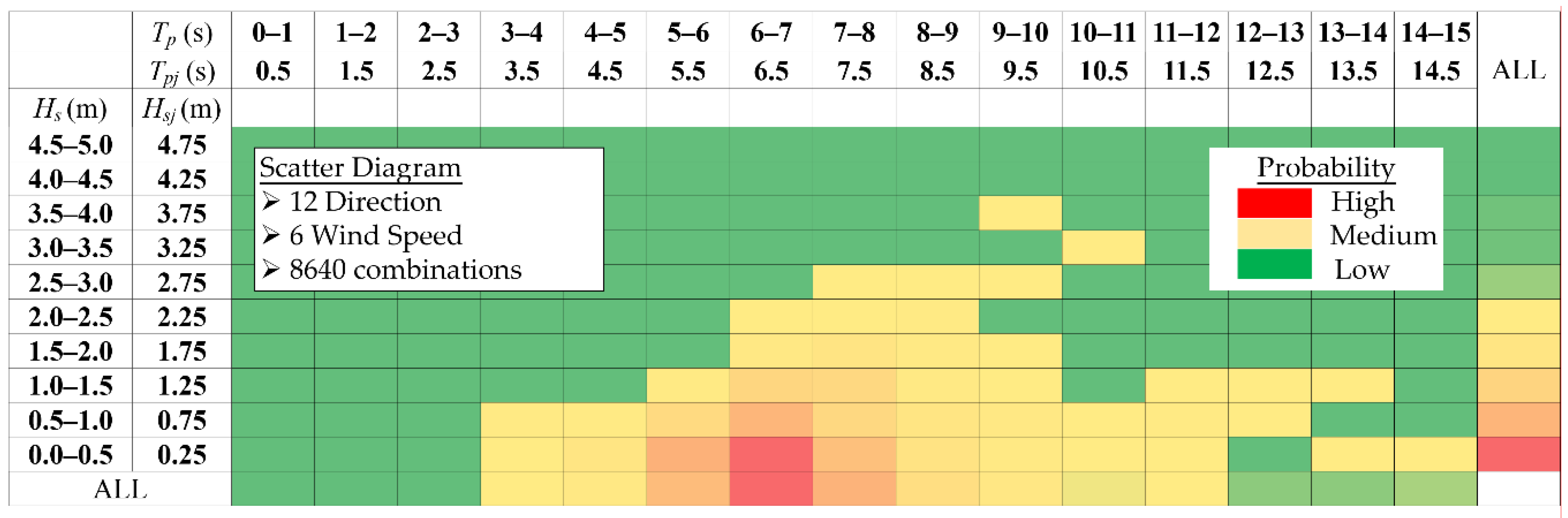
2. Long-Term Environmental Statistics and Sampling
2.1. Grid-Based Method
2.2. MC Method
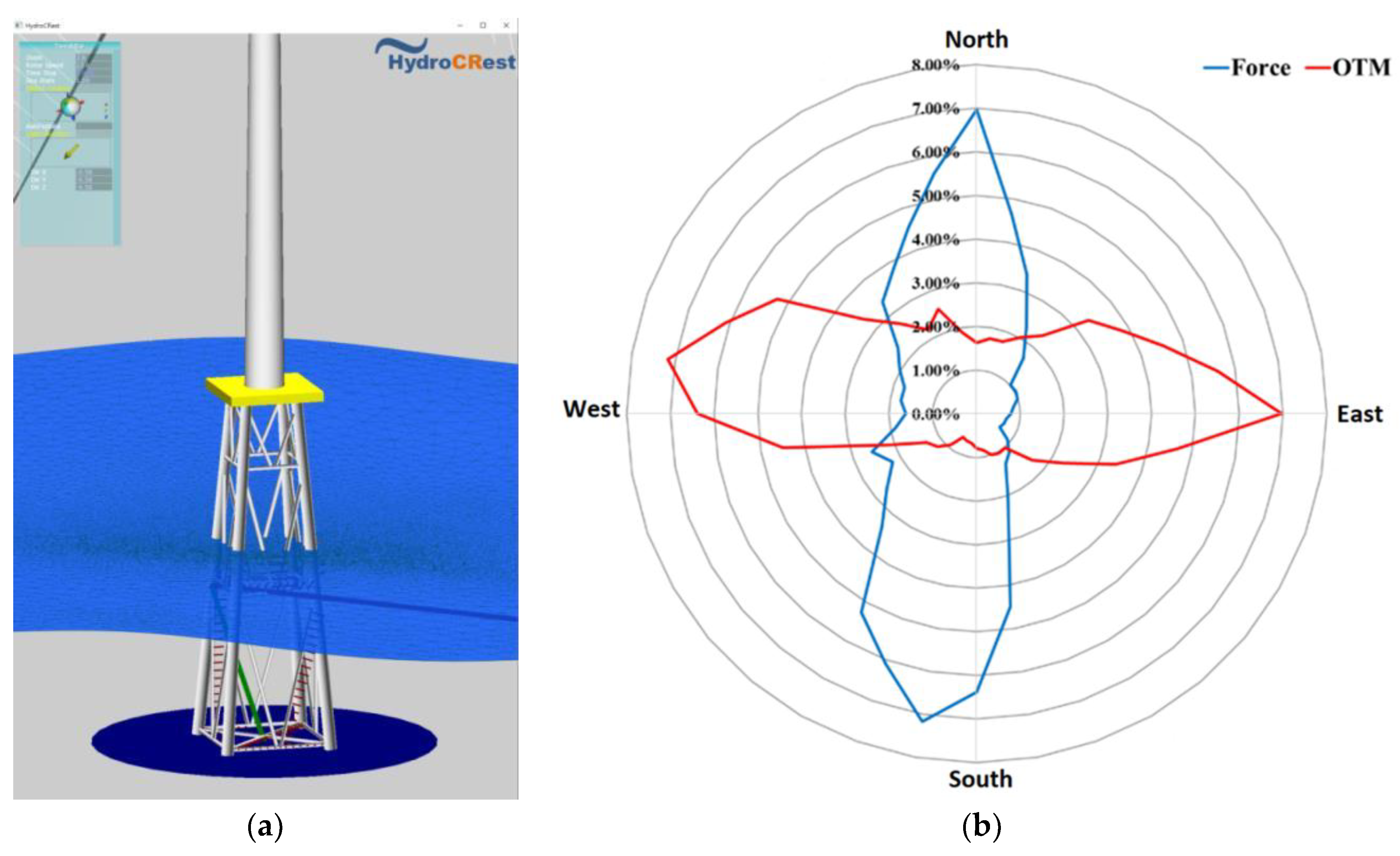
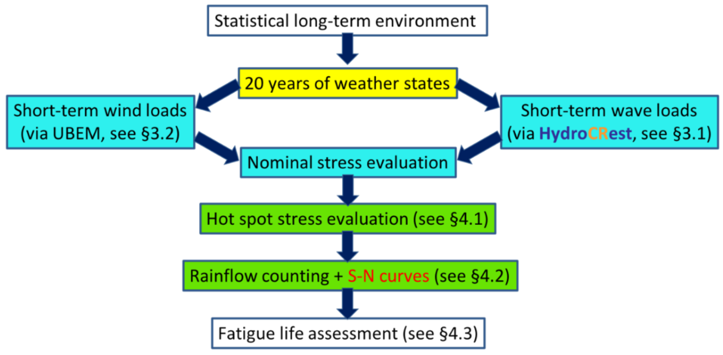
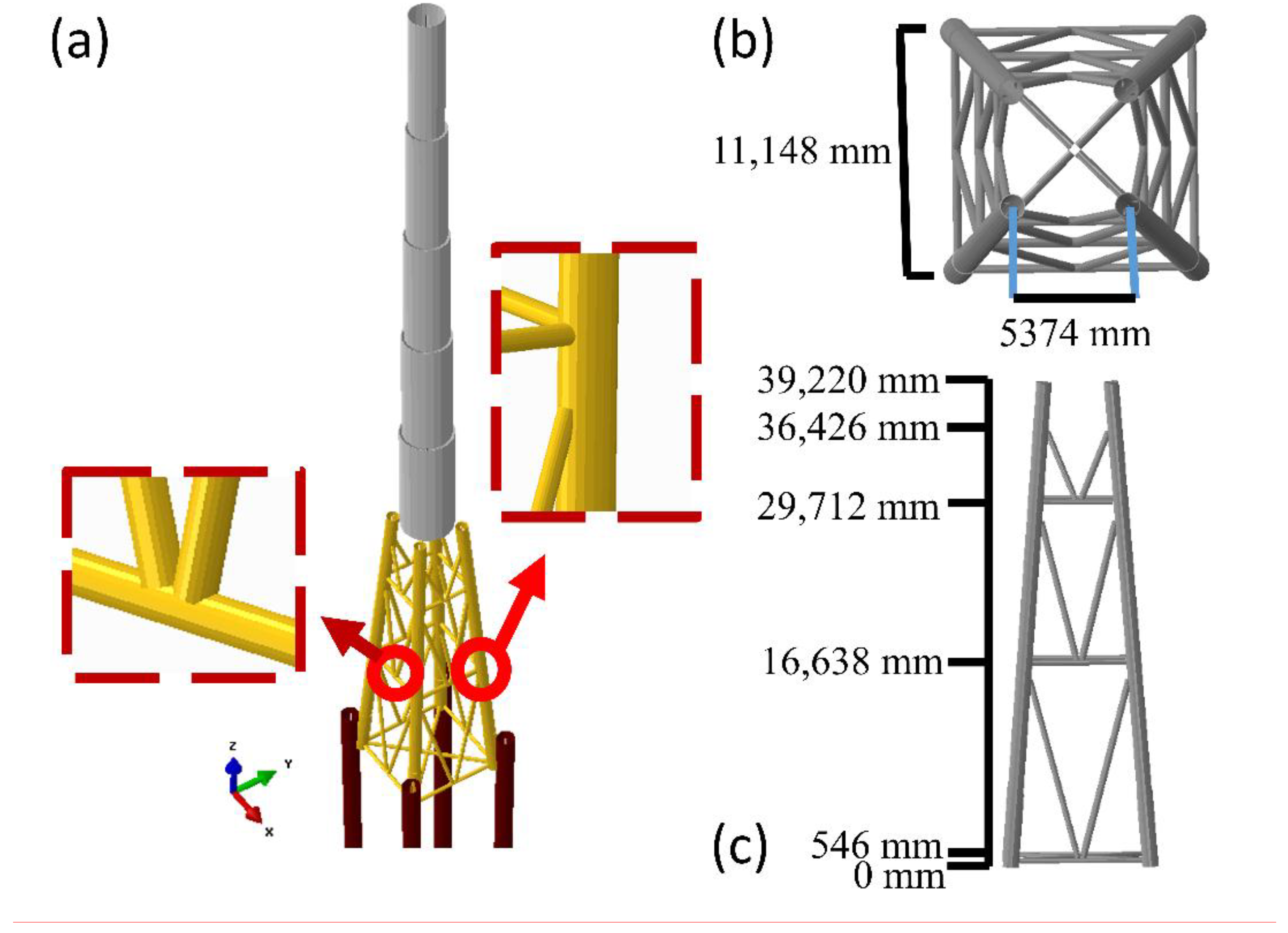
3. Substructure Model Description and Load Generation
3.1. Sea Loads
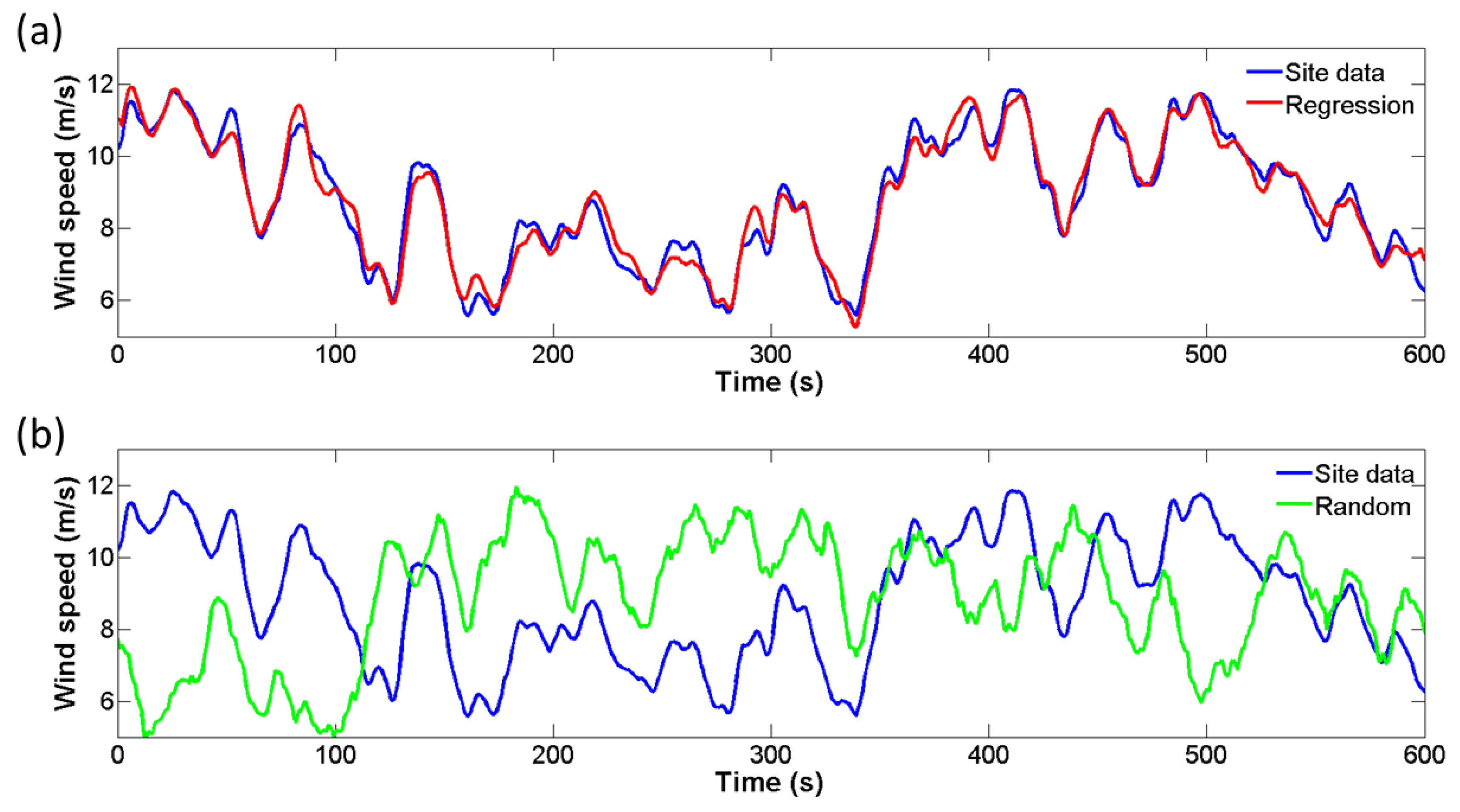
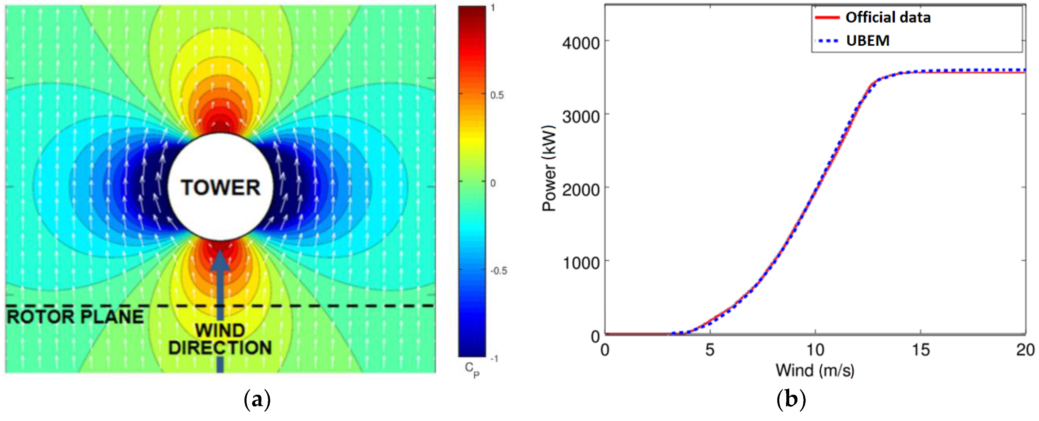
3.2. Wind Loads
4. Fatigue Lifetime Assessment
4.1. Hot-Spot Stress Evaluation
4.2. S–N Curve and Welding Effect
4.3. Fatigue Damage Calculation
5. Results and Discussion
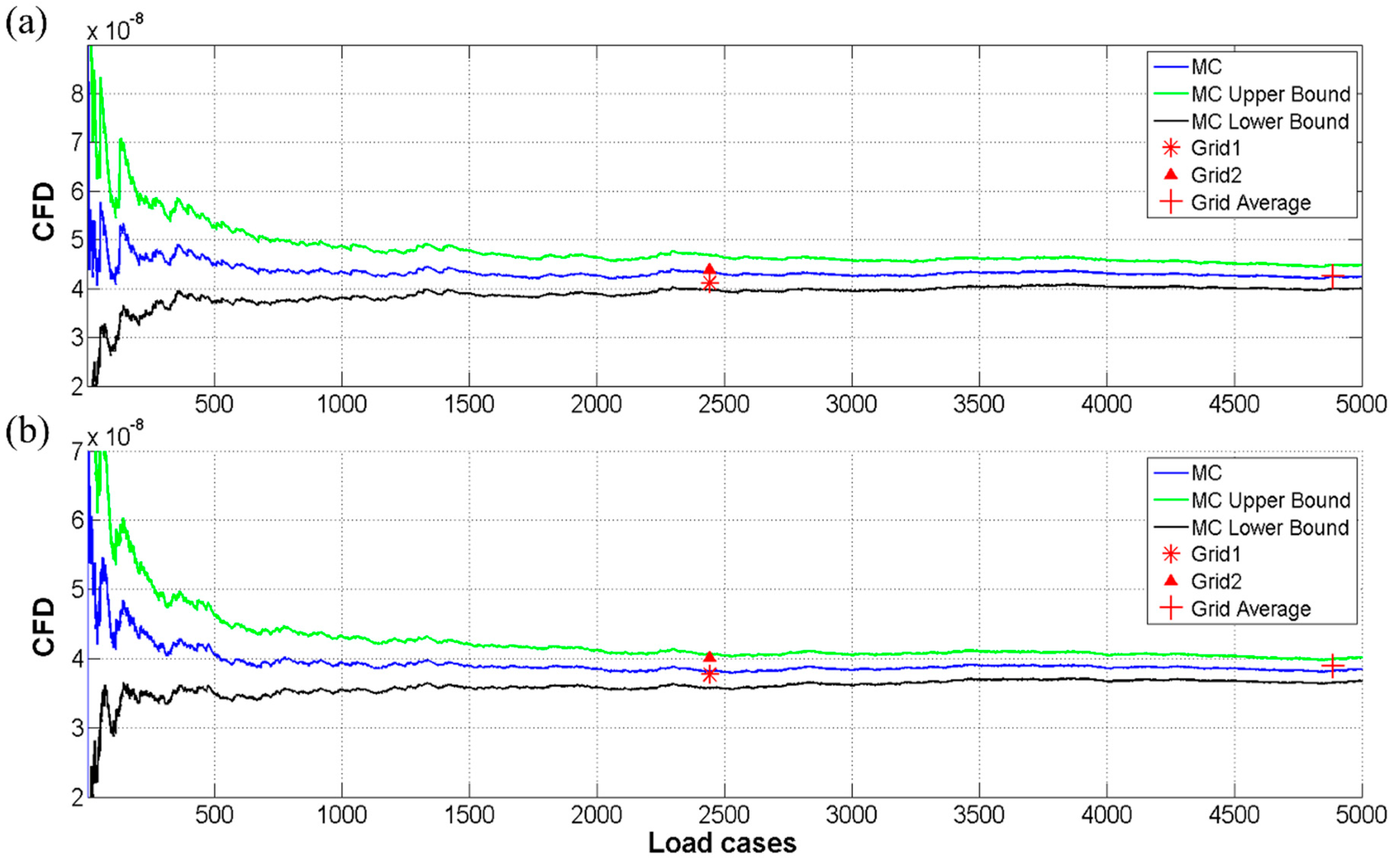
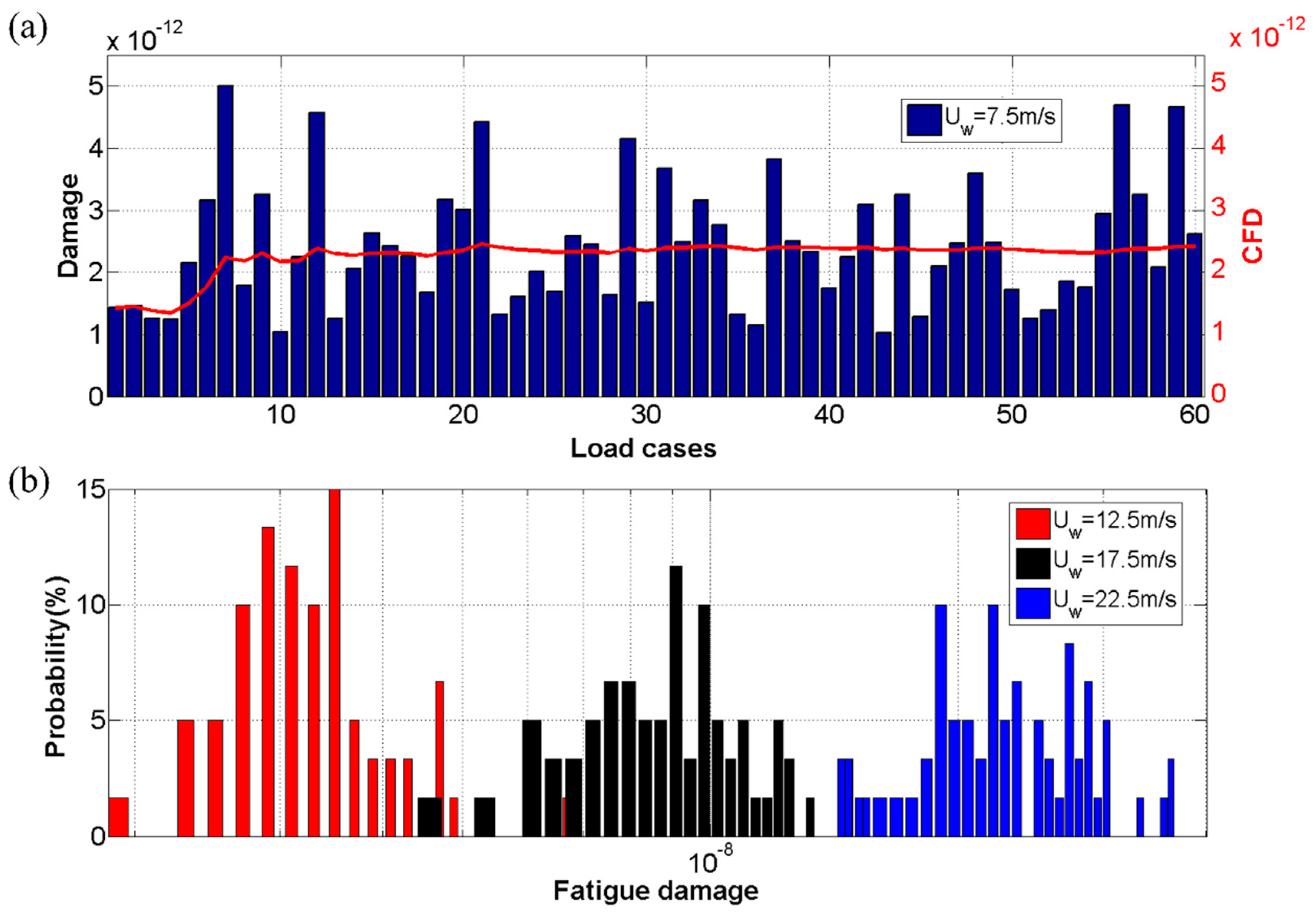
5.1. Uncertainty of Fatigue Damage
5.2. High-Dimensional Fatigue Analysis
6. Concluding Remarks
Author Contributions
Funding
Acknowledgments
Conflicts of Interest
References
- Li, K.; Bian, H.; Liu, C.; Zhang, D.; Yang, Y. Comparison of geothermal with solar and wind power generation systems. Renew. Sustain. Energy Rev. 2015, 42, 1464–1474. [Google Scholar] [CrossRef]
- GWEC. Global Wind Power: 2017 Market and Outlook to 2022. 2017. Available online: http://cdn.pes.eu.com/v/20160826/wp-content/uploads/2018/06/PES-W-2-18-GWEC-PES-Essential-1.pdf (accessed on 19 September 2018).
- Dong, W.; Moan, T.; Gao, Z. Long-term fatigue analysis of multi-planar tubular joints for jacket-type offshore wind turbine in time domain. Eng. Struct. 2011, 33, 2002–2014. [Google Scholar] [CrossRef]
- Vugts, J. Fatigue damage assessments and the influence of wave directionality. Appl. Ocean Res. 2005, 27, 173–185. [Google Scholar] [CrossRef]
- Zwick, D.; Muskulus, M. The simulation error caused by input loading variability in offshore wind turbine structural analysis. Wind Energy 2015, 18, 1421–1432. [Google Scholar] [CrossRef]
- Veldkamp, D. A probabilistic evaluation of wind turbine fatigue design rules. Wind Energy 2008, 11, 655–672. [Google Scholar] [CrossRef] [Green Version]
- Stacey, A.; Sharp, J. Safety factor requirements for the offshore industry. Eng. Fail. Anal. 2007, 14, 442–458. [Google Scholar] [CrossRef]
- Dong, W.; Moan, T.; Gao, Z. Fatigue reliability analysis of the jacket support structure for offshore wind turbine considering the effect of corrosion and inspection. Reliab. Eng. Syst. Saf. 2012, 106, 11–27. [Google Scholar] [CrossRef]
- Dong, W.; Moan, T.; Gao, Z. Statistical Uncertainty Analysis in the Long-Term Distribution of Wind-and Wave-Induced Hot-Spot Stress for Fatigue Design of Jacket Wind Turbine Based on Time Domain Simulations. In Proceedings of the ASME 2011 30th International Conference on Ocean, Offshore and Arctic Engineering (OMAE 2011), Rotterdam, The Netherlands, 19–24 June 2011; Volume 5, pp. 407–417. [Google Scholar]
- Pang, T.; Yang, Y.; Zhao, D. Convergence studies on Monte Carlo methods for pricing mortgage-backed securities. Int. J. Financ. Stud. 2015, 3, 136–150. [Google Scholar] [CrossRef]
- Bilionis, D.V.; Vamvatsikos, D. Fatigue analysis of an offshore wind turbine in Mediterranean Sea under a probabilistic framework. In Proceedings of the VI International Conference on Computational Methods in Marine Engineering (MARINE 2015), Rome, Italy, 15–17 June 2015. [Google Scholar]
- Vahdatirad, M.; Andersen, L.V.; Ibsen, L.B.; Sørensen, J.D. Stochastic dynamic stiffness of a surface footing for offshore wind turbines: Implementing a subset simulation method to estimate rare events. Soil Dyn. Earthq. Eng. 2014, 65, 89–101. [Google Scholar] [CrossRef]
- Dong., Y.; Soares., C.G. Uncertainty analysis of local strain and fatigue crack initiation life of welded joints under plane strain condition. In Proceedings of the 6th international conference on marine structures (MARSTRUCT 2017), Lisbon, Portugal, 8–10 May 2017; pp. 349–360. [Google Scholar]
- Jensen, J.J. Fatigue damage estimation in non-linear systems using a combination of Monte Carlo simulation and the First Order Reliability Method. Mar. Struct. 2015, 44, 203–210. [Google Scholar] [CrossRef]
- Horn, J.-T.H.; Jensen, J.J. Reducing uncertainty of Monte Carlo estimated fatigue damage in offshore wind turbines using FORM. In Proceedings of the 13th International Symposium on PRActical Design of Ships and Other Floating Structures (PRADS’ 2016), Technical University of Denmark (DTU), Copenhagen, Denmark, 4–8 September 2016. [Google Scholar]
- Graf, P.A.; Stewart, G.; Lackner, M.; Dykes, K.; Veers, P. High-throughput computation and the applicability of Monte Carlo integration in fatigue load estimation of floating offshore wind turbines. Wind Energy 2016, 19, 861–872. [Google Scholar] [CrossRef]
- Ragan, P.; Manuel, L. Comparing estimates of wind turbine fatigue loads using time-domain and spectral methods. Wind Eng. 2007, 3, 83–99. [Google Scholar] [CrossRef]
- Kvittem, M.I.; Moan, T. Frequency versus time domain fatigue analysis of a semisubmersible wind turbine tower. J. Offshore Mech. Arct. Eng. 2015, 137, 011901. [Google Scholar] [CrossRef] [Green Version]
- International Electrotechnical Commission (IEC). IEC61400-3—Wind Turbines Part III: Design Requirements for Offshore Wind Turbines; IEC: Geneva, Switzerland, 2009. [Google Scholar]
- Det Norske Veritas—Germanischer Lloyd (DNV GL). Recommended Practice DNVGL-ST-0126—Support Structures for Wind Turbines; DNV GL: Berum, Norway, 2016. [Google Scholar]
- Niesłony, A. Determination of fragments of multiaxial service loading strongly influencing the fatigue of machine components. Mech. Syst. Signal Process. 2009, 23, 2712–2721. [Google Scholar] [CrossRef]
- Det Norske Veritas—Germanischer Lloyd (DNV GL). Recommended Practice DNV-RP-C203—Fatigue Design of Offshore Steel Structures; DNV GL: Høvik, Norway, 2016. [Google Scholar]
- International Electrotechnical Commission (IEC). IEC61400-1—Wind Turbines—Part I: Design Requirements; IEC: Geneva, Switzerland, 2005. [Google Scholar]
- Hasselmann, K.; Barnett, T.; Bouws, E.; Carlson, H.; Cartwright, D.; Enke, K.; Ewing, J.; Gienapp, H.; Hasselmann, D.; Kruseman, P. Measurements of wind-wave growth and swell decay during the Joint North Sea Wave Project (JONSWAP). Ergänzung zur Deut. Hydrogr. Z. 1973, 12, 1–95. [Google Scholar]
- Fréchot, J. Realistic simulation of ocean surface using wave spectra. In Proceedings of the First International Conference on Computer Graphics Theory and Applications (GRAPP 2006), Setúbal, Portugal, 25–28 February 2006; pp. 76–83. [Google Scholar]
- Kristensen, L.; Jensen, G.; Hansen, A.; Kirkegaard, P. Field Calibration of Cup Anemometers; Riso National Laboratory: Copenhagen, Denmark, 2001. [Google Scholar]
- Hansen, M.O.L. Aerodynamics of Wind Turbines, 2nd ed.; Earthscan: London, UK, 2008; pp. 107–124. ISBN 978-1-84407-438-9. [Google Scholar]
- Siemens. Thoroughly Tested, Utterly Reliable. Siemens Wind Turbine swt-3.6-120. 2011. Available online: https://www.siemens.com/content/dam/internet/siemens-com/global/market-specific-solutions/wind/data_sheets/data-sheet-wind-turbine-swt-3-6-120.pdf (accessed on 3 September 2018).
- Efthymiou, M. Development of SCF formulae and generalised influence functions for use in fatigue analysis. In Proceedings of the Recent Developments in Tubular Joint Technology, OTJ ’88, London, UK, 4–5 October 1988. [Google Scholar]
- Fatemi, A.; Yang, L. Cumulative fatigue damage and life prediction theories: A survey of the state of the art for homogeneous materials. Int. J. Fatigue 1998, 20, 9–34. [Google Scholar] [CrossRef]
- Niesłony. Rainflow Counting Algorithm, Version 1.2. Rain Flow Counting Method, Set of Functions with User Guide for Use with MATLAB. 2010. Available online: http://www.mathworks.com/matlabcentral/fileexchange/3026 (accessed on 25 September 2018).


| Wind Speed | 7.5 m/s | 12.5 m/s | 17.5 m/s | 22.5 m/s |
|---|---|---|---|---|
| Maximum (MAX) | ||||
| Minimum (MIN) | ||||
| Average (AVG) | ||||
| MAX/AVG | 206.9% | 224.6% | 168.2% | 154.0% |
| MIN/AVG | 42.1% | 52.5% | 47.0% | 59.6% |
| STD | ||||
| CV | 0.420 | 0.288 | 0.249 | 0.218 |
| Wave Height | 0.75 m | 1.25 m | 1.75 m |
|---|---|---|---|
| Maximum (MAX) | |||
| Minimum (MIN) | |||
| Average (AVG) | |||
| MAX/AVG | 231.0% | 225.2% | 325.0% |
| MIN/AVG | 38.9% | 32.3% | 35.1% |
| STD | |||
| CV | 0.407 | 0.419 | 0.487 |
© 2018 by the authors. Licensee MDPI, Basel, Switzerland. This article is an open access article distributed under the terms and conditions of the Creative Commons Attribution (CC BY) license (http://creativecommons.org/licenses/by/4.0/).
Share and Cite
Chian, C.-Y.; Zhao, Y.-Q.; Lin, T.-Y.; Nelson, B.; Huang, H.-H. Comparative Study of Time-Domain Fatigue Assessments for an Offshore Wind Turbine Jacket Substructure by Using Conventional Grid-Based and Monte Carlo Sampling Methods. Energies 2018, 11, 3112. https://doi.org/10.3390/en11113112
Chian C-Y, Zhao Y-Q, Lin T-Y, Nelson B, Huang H-H. Comparative Study of Time-Domain Fatigue Assessments for an Offshore Wind Turbine Jacket Substructure by Using Conventional Grid-Based and Monte Carlo Sampling Methods. Energies. 2018; 11(11):3112. https://doi.org/10.3390/en11113112
Chicago/Turabian StyleChian, Chi-Yu, Yi-Qing Zhao, Tsung-Yueh Lin, Bryan Nelson, and Hsin-Haou Huang. 2018. "Comparative Study of Time-Domain Fatigue Assessments for an Offshore Wind Turbine Jacket Substructure by Using Conventional Grid-Based and Monte Carlo Sampling Methods" Energies 11, no. 11: 3112. https://doi.org/10.3390/en11113112