Modeling Aggregate Hourly Energy Consumption in a Regional Building Stock


Faculty of Environmental Sciences and Natural Resource Management, Norwegian University of Life Sciences, P.O. Box 5003, N-1432 Ås, Norway
*
Author to whom correspondence should be addressed.
Energies 2018, 11(1), 78; https://doi.org/10.3390/en11010078
Submission received: 21 November 2017
/
Revised: 19 December 2017
/
Accepted: 26 December 2017
/
Published: 29 December 2017
Abstract
:Sound estimates of future heat and electricity demand with high temporal and spatial resolution are needed for energy system planning, grid design, and evaluating demand-side management options and polices on regional and national levels. In this study, smart meter data on electricity consumption in buildings are combined with cross-sectional building information to model hourly electricity consumption within the household and service sectors on a regional basis in Norway. The same modeling approach is applied to model aggregate hourly district heat consumption in three different consumer groups located in Oslo. A comparison of modeled and metered hourly energy consumption shows that hourly variations and aggregate consumption per county and year are reproduced well by the models. However, for some smaller regions, modeled annual electricity consumption is over- or underestimated by more than 20%. Our results indicate that the presented method is useful for modeling the current and future hourly energy consumption of a regional building stock, but that larger and more detailed training datasets are required to improve the models, and more detailed building stock statistics on regional level are needed to generate useful estimates on aggregate regional energy consumption.
1. Introduction
1.1. Background
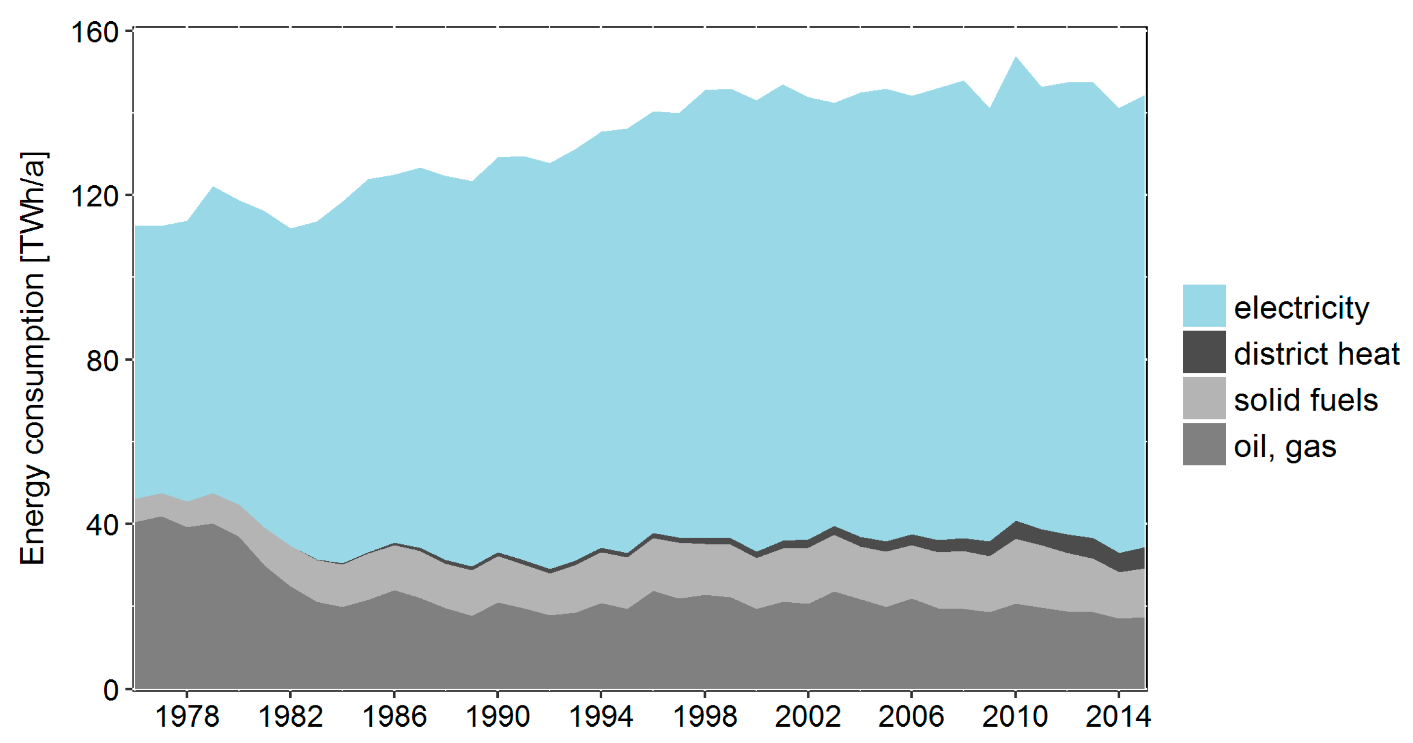
Stationary energy consumption in Norway has been steadily increasing over the last quarter of the 20th century, and due to the availability of hydropower, electricity has been the most important energy carrier (Figure 1). However, electricity consumption has flattened since the year 2000. Plausible reasons for this development include higher energy prices, stricter building codes with respect to energy demand, reduced heat demand due to a milder climate, more energy-efficient electric appliances, the increased use of heat pumps, and the closing down of factories in energy-intensive industries. Although total consumption of district heat is comparably low, it increased by 40% between 2011 and 2016, while the consumption of solid fuels, oil, and gas was slightly reduced [1].
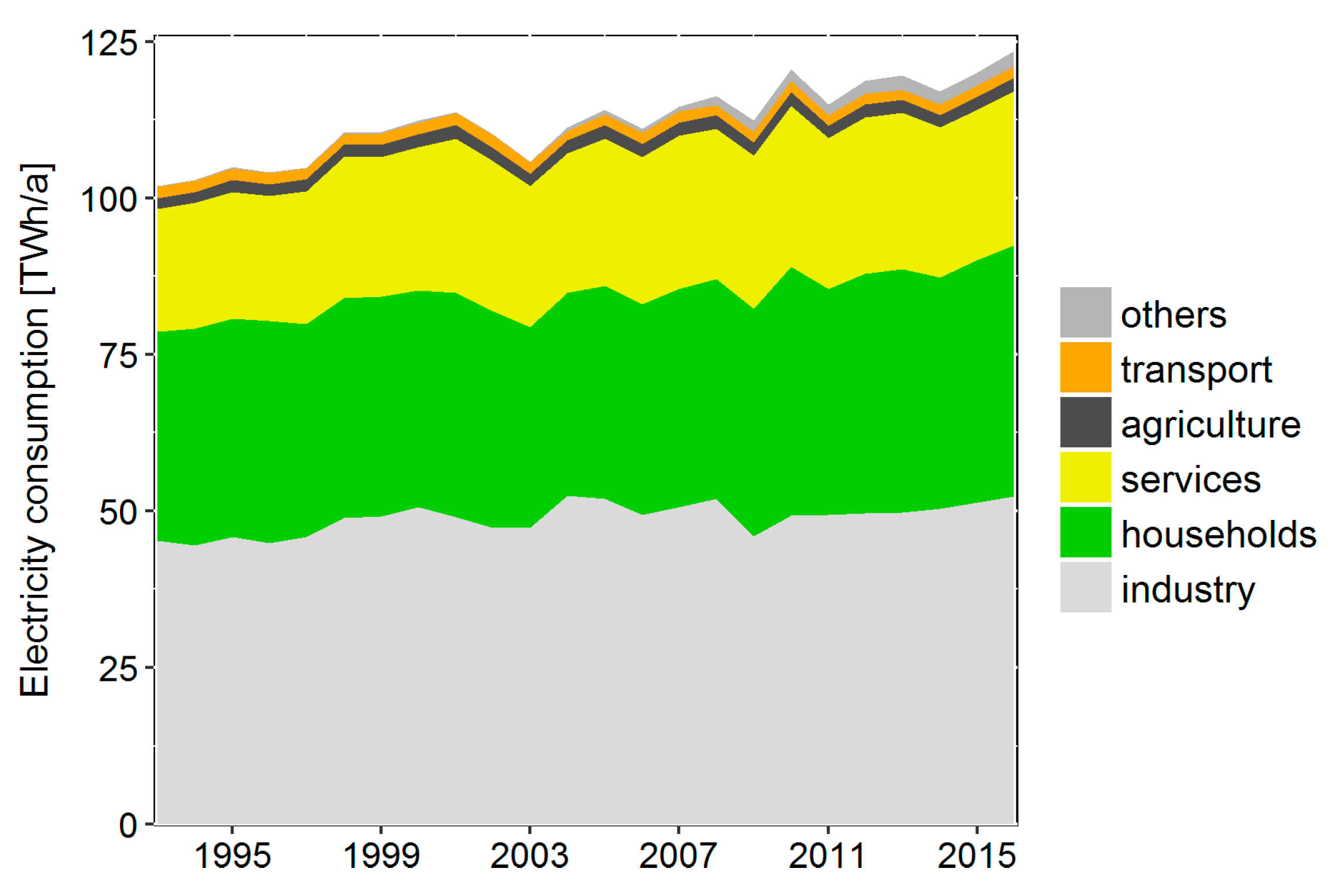
The industrial sector, including energy-intensive branches like aluminum and ferro-alloys production and wood processing, represents the largest electricity consumer; however, its consumption exhibited a significant reduction in 2009 (Figure 2), which can be explained by the reduction in demand for products like steel and aluminum caused by the international financial crisis [2]. Households account for about one third, and services (including construction) for about one fifth of total electricity consumption, while agriculture (including fishing and forestry), transport, and other sectors combined account for about 5% [3]. As a result of low electricity prices, electrical energy is largely used for space and domestic water heating in Norway, and therefore part of the electricity consumption is strongly correlated with outdoor temperature. As such, the consumption peak in 2010 and the consumption low in 2014 can be explained by unusually cold and warm heating periods in 2010 and 2014.
In contrast to most EU-countries, where electricity is still mainly generated in thermal power plants and electricity prices are comparably high, electrical energy in Norway is broadly used for space and domestic water heating; this explains the typically high electricity shares in total consumption, particularly in the household and service sectors. In recent years, the use of heat pumps for space heating purposes has increased significantly. While heat pumps were installed in only 4% of dwellings in 2004, the share was 27% in 2012 (and even 44% in single family houses) [5].
Milder winters, stricter energy standards in building codes, and rehabilitation of existing buildings might contribute to reduce heat demand in buildings in the future, whereas higher temperatures during summer may lead to increased cooling energy demand. Moreover, population growth entails a growing residential and non-residential building stock—and therefore increased energy consumption for electric appliances as well as space heating and cooling—while the increased energy efficiency of electric appliances and decreased floor space per employee or resident contributes to reduced energy consumption per capita. Ideally, models used for energy demand forecasting should be able to take into account these factors.
The introduction of area-wide smart metering yields enormous amounts of highly resolved micro-level energy consumption data that can be utilized in combination with weather data and cross-sectional data, collected by customer surveys—to develop more precise prediction models and detailed analyses of the drivers of energy consumption. Consumption models with comparably high temporal and spatial resolutions are useful tools in evaluating and implementing demand-side management measures that can forward the integration of renewable energy carriers into the energy system. Moreover, forecasts of regional hourly energy consumption can provide estimates for electric or thermal loads, which are crucial for designing power lines, district heating networks, and decentralized generators of heat and power. Thus, forecasts represent valuable information for energy system planning where the required temporal, spacial, and sectoral resolutions depend on the scope of application. For instance, Rosenberg et al. [6] develop long-term projections of energy demand in different Norwegian sectors by identifying important drivers of energy consumption within each sector, calculating energy consumption per driver (intensities) for a base year, and calculating projected energy demand based on assumed changes in intensities and drivers. Seljom et al. [7] model the changes in annual heating and cooling energy demand in Norway from 2005 to 2050 under different outdoor temperature scenarios, using a degree-day approach as well as a more sophisticated bottom-up building physics model for one of the scenarios. Energy demand for heating is estimated to decrease by 9–17% depending on the corresponding scenarios, while cooling energy demand is estimated to slightly increase [7]. Andersen et al. [8,9] identify hourly electricity consumption profiles for different consumer categories in Denmark and estimate weights indicating the impact of each category on aggregate hourly electricity consumption in different Danish regions. The method is used for forecasting hourly electricity consumption on a regional level, based on national projections on electricity consumption in each category.
1.2. Methods for Modeling Aggregate Hourly Energy Consumption
Energy consumption models can be divided into bottom-up and top-down models [10,11]. Top-down models usually rely on historic values of aggregate consumption and macroeconomic variables and often only need few and easily available input variables. However, changes in disaggregate consumption caused by the use of different electric appliances or heating equipment cannot be implemented. Bottom-up models for aggregate energy consumption typically model energy consumption of individual buildings or end-use appliances and then aggregate consumption over the entire building stock. Input variables for bottom-up models might be consumer-specific variables, such as building type, dwelling or building size, building age, information on different appliances and heating equipment, as well as weather data. Bottom-up models can further be divided into statistical models and engineering models. Bottom-up engineering models are developed based on consumption characteristics of single end-use appliances combined with detailed information on, e.g., building physics, occupancy patters, and number of different appliances [12,13,14,15]. In theory, no historical consumption data is necessary to develop engineering models, and the effects of new technologies can be implemented and analyzed. Disadvantages of engineering models are that consumer behavior is often based on assumptions, and that developing and applying the models often requires a high level of expertise. Statistical bottom-up models for residential consumption are typically developed based on historic consumption data of a sample of representative consumers (or buildings) and additional variables describing those consumers. Compared to engineering models, statistical bottom-up models are less dependent of detailed physical data and assumptions regarding user behavior [16,17]. Common statistical bottom-up modeling techniques are regression and artificial neural networks (ANN). The latter represents a more sophisticated, data-driven method for modeling and forecasting energy demand and has become increasingly common during recent years [18,19,20,21,22,23,24]. In contrast to regression models, ANN does not produce coefficients that can be easily interpreted, and the method usually requires high developer skills and powerful computing resources.
Advantages of regression models are their simplicity and the straightforward interpretation of regression coefficients. An analysis of variance yields the contribution of each explanatory variable to total explained variance, which facilitates an assessment of different impact factors. Since modeled energy consumption consists of several individual components, each represented by a parameter estimate and the corresponding explanatory variable, it can be broken down accordingly to analyze how much different factors contribute to modeled consumption. Including outdoor temperature (or heating degree day) as an explanatory variable enables estimating how much energy is used for space-heating. Moreover, with a simple model structure, modeling time-aggregate (e.g., individual daily or yearly energy consumption), and sample-aggregate energy consumption (i.e., hourly consumption of several consumers), or a combination of both is easily performed using linear regression models. Many bottom-up regression models for energy demand modeling rely on the Princeton Scorekeeping Method [25], which describes the fundamental correlation between outdoor temperature and heating energy consumption. Recent studies using regression for modeling and predicting energy consumption often analyze hourly or sub-hourly energy meter data [26,27,28,29,30,31,32,33].
1.3. Objectives
The objective of this study is to show how smart meter data on energy consumption in buildings can be combined with cross-sectional building information, weather data, and calendric data to model aggregate hourly energy consumption of a regional building stock connected to the household and service sectors. We develop regression models for individual hourly electricity consumption in different building categories within both sectors and use official population and building stock statistics to derive useful input data to model aggregate hourly electricity consumption in each Norwegian county. Moreover, the method is applied to model aggregate hourly district heat consumption in three consumer categories in Oslo. Finally, we discuss potential model improvements and data requirements for forecasting regional hourly energy demand based on our modeling approach.
While the general modeling approach for individual hourly energy consumption is described in previous work [34,35,36], this study aims to model regional aggregate hourly energy consumption by slightly adapting the existing models, including further building categories, as well as to describe how suitable input data to the aggregate models can be gathered and processed.
2. Data and Methods
2.1. Model Setup
The regression models used in this study are based on panel data, consisting of hourly energy meter data, calendric and weather data, as well as cross-sectional data, providing information on the individual electricity or district heat consumers. The household electricity model is based on hourly electricity meter data from several hundred household customers in Buskerud country, and the corresponding cross-sectional data were gathered by a survey performed in 2013. A detailed description of how the method of Pooled Ordinary Least Squares (Pooled OLS) is applied to this panel dataset can be found in [34,35]. The models for district heat and electricity consumption in the service sector are built accordingly and are based on meter data from consumers located in Oslo, combined with cross-sectional data from the Norwegian energy label database; models for office buildings and schools are described in [36]. Compared with the household dataset on electricity consumption, the sample size of the corresponding datasets on non-residential buildings is considerably lower (between <10 and 30 observations, depending on building category and energy carrier (electricity or district heat)). Moreover, available cross-sectional data on non-residential buildings are limited and mainly include building category and floor space. Following the same method, a model for hourly district heat consumption in apartment buildings located in Oslo is developed, and the corresponding cross-sectional data were gathered via a brief e-mail survey in 2017. The sample includes 16 apartment buildings.
All models are set up according to Equation (1). The independent variable —i.e., modeled energy consumption of consumer i in hour h—is calculated based on intercept estimate , parameter estimates , and the explanatory variables .
All explanatory variables that are included in the models for hourly electricity consumption in households and service sector are listed in Table A1 and Table A2, respectively. While most variables are categorical, floor space and heating degree day (HDD) are continuous variables. Since not all variables are equally important in the different models for electricity consumption in the service sector and for district heat consumption, Table A3 and Table A4 show which variables from Table A2 are used in which model. Parameter estimates ( and for each model can be obtained by contacting the authors.
Heating and cooling degree day (HDD and CDD) are defined as the differences between daily mean outdoor temperature and corresponding base temperatures tb,HDD and tb,CDD , and can only have positive values by definition (Equations (2) and (3)).
In this study, different base temperatures for HDD in household model (tb,households,HDD = 17 °C) and service sector models (tb,services,HDD = 14 °C) are used. These assumptions are based on previous work, where the temperature-dependency of energy consumption in residential and non-residential buildings is discussed [13]. Different base temperatures can be partially explained by higher internal heat gains in non-residential buildings. CDD is only included in the models for electricity consumption in office buildings and shops, and we choose a base temperature of tb,CDD = 14 °C as well, which is also based on previous work [36].
In addition, we introduce an auxiliary variable first differences in heating degree days (HDD1st), as the difference in HDD between two consecutive days (Equation (4)).
2.2. Decomposing Hourly Electricity Consumption
By including temperature variables HDD and HDD1st, modeled electricity consumption can be broken down into an HDD-independent and an HDD-dependent component. The HDD-dependent component is the sum of all components containing HDD or HDD1st and can be interpreted as space heating consumption. The sum of all remaining components can be interpreted as consumption for electric appliances, including electrically heated hot water tanks and space cooling equipment (i.e., electricity-bound consumption). The decomposition method is described in detail in [35].
2.3. Modeling Hourly Electricity Consumption
We use separate models for different building categories—namely dwellings, office buildings, schools and universities, kindergartens, shops and stores, and nursing homes—and a category representing hotels, restaurants, and cultural buildings. Each building category represents a consumer category (i.e., dwellings represent households, office buildings represent all services that are office-based, etc.). An overview of the different models for building and consumer categories, including references that describe the corresponding data and models, is given in Table 1.
For office buildings as well as schools and university buildings, we use separate models for buildings with and without electric heating, respectively, while for the remaining categories, only one model is available per category (due to limited meter data). Modeled electricity consumption is broken down into two components for electricity-bound appliances—including domestic water heating—and space heating purposes, respectively (see Ch. 2.2). Electricity consumption in buildings or dwellings with non-electric heating is calculated by setting the HDD-dependent component (i.e., modeled consumption for electric space heating) equal to zero.
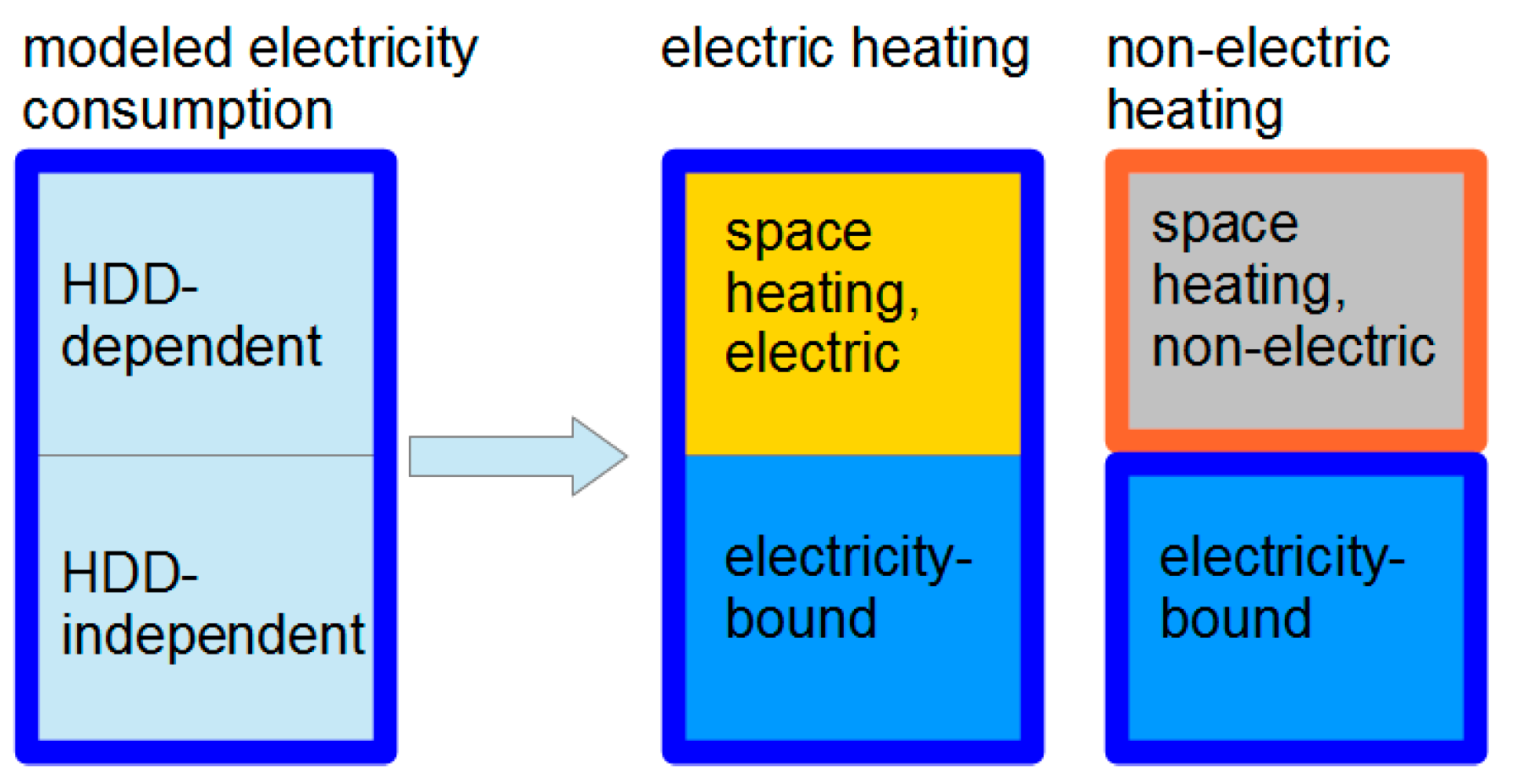
The following graphic (Figure 3) illustrates how the models based on electricity meter data (Table 1) are used to model electricity-bound and space heating energy consumption in buildings with either electric heating or non-electric heating. In buildings with electric space heating, electricity is the only energy carrier (thick blue border), while in buildings with non-electric space heating electricity and other energy carriers (thick orange border) are used. Examples for other energy carriers are biomass (e.g., firewood) or district heat. Energy consumption provided by other energy carriers is assumed to be equal to electricity consumption used for space heating in a comparable building, although hourly heat production patterns of, for instance, wood stoves and electric heaters certainly differ.
2.4. Modeling Hourly District Heat Consumption
Based on meter data from buildings located in Oslo, separate regression models for individual hourly district heat consumption in three consumer groups are developed (Table 2), following the method described in Section 2.1. The models for office buildings and schools (representing education) are documented in [36].
2.5. Modeling Aggregate Regional Hourly Energy Consumption
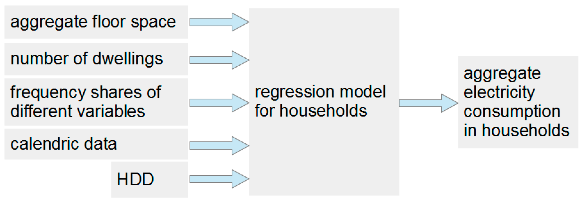
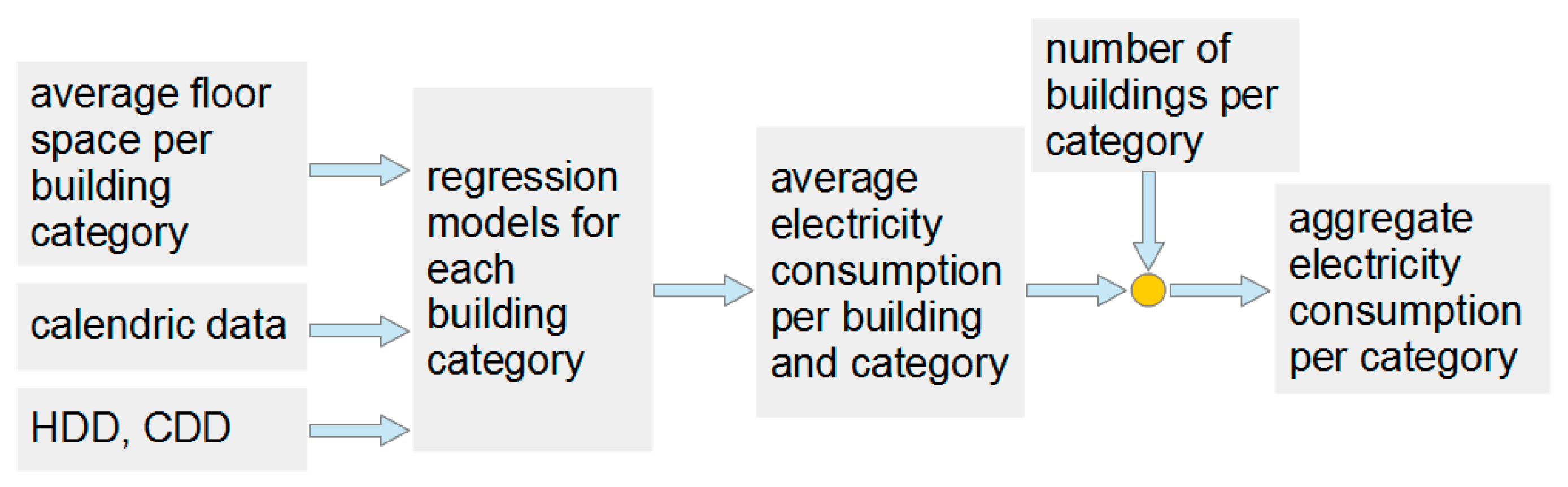
Each model calculates hourly energy consumption for an individual consumer (e.g., a household, a school, or an office building). In order to calculate aggregate hourly energy consumption in an entire building category—e.g., all residential buildings, schools, and office buildings in a specific region (county) and time period—the following steps are performed as illustrated in Figure 4 and Figure 5.
All buildings and dwellings in each region are assumed to be “in use” (i.e., not empty or abandoned). For the household sector (Figure 4), aggregate hourly electricity consumption is directly calculated by using aggregate input data (i.e., total number and aggregate floor space of all dwellings in a specific region), calculated based on official statistics [37,38,39,40,41,42,43]. Different dummy variables (e.g., indicating the number of residents or the use of electric appliances and heating equipment) are given as percent shares, and are mainly based on survey response data from Buskerud county (survey items are included in [35]. Chosen input data for each county can be obtained from the corresponding author).
For the service sector (Figure 5), we model hourly electricity consumption in an average building within each category and multiply the result with the total number of buildings. The average floor space of different non-residential buildings is calculated based on mean values derived from the Norwegian energy label database (only data from buildings located in Oslo are used).
Aggregate hourly district heat consumption in Oslo in three different consumer groups is estimated according to Figure 5 as well. The average hourly consumption in each consumer group is estimated based on average floor space values and then multiplied by the total number of buildings supplied with district heat.
3. Input Data
3.1. Number and Size of Buildings and Dwellings
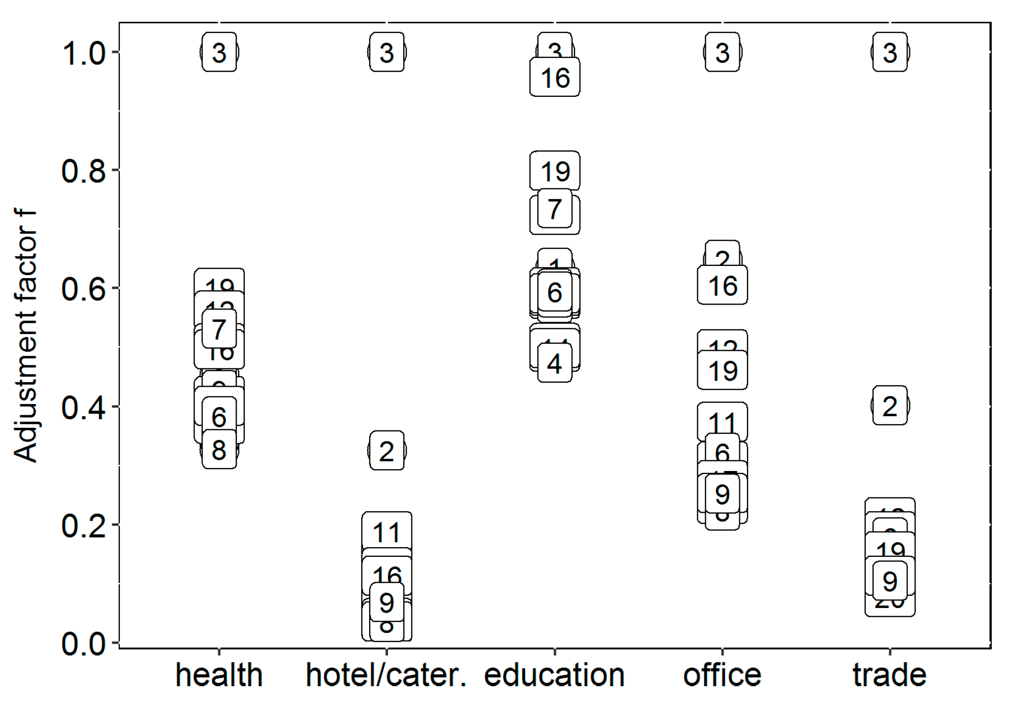
The models used in this study calculate electricity consumption per dwelling (residential sector) or building (service sector). In order to estimate aggregate regional consumption, we need sound estimates of the number of dwellings and non-residential buildings per region. Continental Norway is divided into 19 counties that differ in factors such as population, economic structure, and climate. The number of dwellings is strongly correlated with the number of people living in each county, while the number of non-residential buildings is mainly determined by the number of people working in the corresponding counties. Relatively detailed statistics and historical data are available for the mean floor space of different dwelling types in each county, so we can use these as input data to our household consumption model. For non-residential buildings (i.e., the service sector), no official statistics on floor space are available, so we make assumptions based on data derived from the Norwegian energy label database. The database includes technical information on all buildings that have been assigned an official energy label [44], which is mandatory for almost all non-residential buildings in Norway. Since the database mainly includes buildings located in Oslo, we estimate building floor space for the remaining 18 counties using an adjustment factor (see Section 3.1 and Figure 6).
The number of people living in different types of dwellings varies from county to county [37,38]. While, in most counties, detached houses are the most common type, apartments prevail in Oslo. The number of households is approximately proportional to the number of people living in each county [39,40,41]. The average number of people per household varies between 2.2 and 2.4 for most counties but is only 1.9 for Oslo, which can be explained by the large share of apartments (typically smaller than other dwellings). In this study, we assume the number of households to be equal to the number of dwellings, meaning one household per dwelling.
The number of employees per county (i.e., people working in but not necessarily living in the corresponding county) can be grouped according to different economic branches. Oslo exhibits the highest number of employees, a large percentage of whom work in office-related fields (such as commercial services, finance and insurance, technical and real estate services, and information and communication). In many other regions, the share of people working in health, education, or trade is larger, while the share of office-related branches is correspondingly smaller. As described in Section 2, we use separate regression models for six different building categories, and both the number of buildings and average floor space are needed as cross-sectional input variables to each model.
The number of non-residential buildings is positively correlated with the number of employees; however, while Oslo clearly exhibits the highest number of employees, the absolute number of non-residential buildings in Oslo is comparably low. This leads to the assumption that, on average, non-residential buildings in Oslo are larger compared to buildings in other counties, since there are, on average, more employees per building. In order to illustrate this finding, we define a factor called average employees per building (epb, Equation (5)) for each category (cat) and county (cnty), based on figures from official statistics [42,43].
The adjustment factor f relates the epb–value for each county to the epb-value for Oslo (Equation (6)).
The resulting adjustment factors f (Figure 6) are smallest for trade, hotels and catering, and other services, while highest for education. In the Trondheim area (county 16), the number of employees per building within education is almost as high as in Oslo (county 3), which can be explained by the fact that Norway’s second largest university is located in this county.
Our models for energy consumption in the service sector are based on meter data from Oslo buildings, and mean floor space per category is primarily only available for Oslo, as well. Average floor space for each building category in the remaining 18 counties could in theory be estimated by multiplying average floor space in Oslo by adjustment factor f. However, this would yield very small values for some counties and building categories, so the models would be no longer applicable. In order to correct for assumed differences in building sizes, we instead reduce the number of buildings by multiplying with adjustment factor f, and use average floor space values for Oslo.
3.2. Heating Systems
Heating equipment and heating energy carriers are important factors for modeling energy consumption in Norway. In single-family houses, direct electric heating, often combined with air-to-air heat pumps or wood burning, is most common [5]. In case of a non-electric main heating system (e.g., district heating), some electric heating might still be used. Especially electric floor heating in bathrooms is common, even if the main heating system is non-electric. In Norwegian households, non-electric heating is mainly used in regions with district heating as well as in larger buildings, such as apartment buildings.
Few official statistics regarding energy carriers and heating systems used in residential or non-residential buildings are available, so we must make a number of assumptions. In our consumption models for the service sector, we only distinguish between electric and non-electric heating and assume different shares for each county and each consumer category. In order to obtain input data to our household sector models, we combine official statistics on heating equipment from a national survey conducted in 2001 with our own assumptions, as well as survey results from a previous study [34,35]. Detailed input data for each county can be obtained from the authors.
4. Results
4.1. Electricity Consumption per County, Sector, and Year
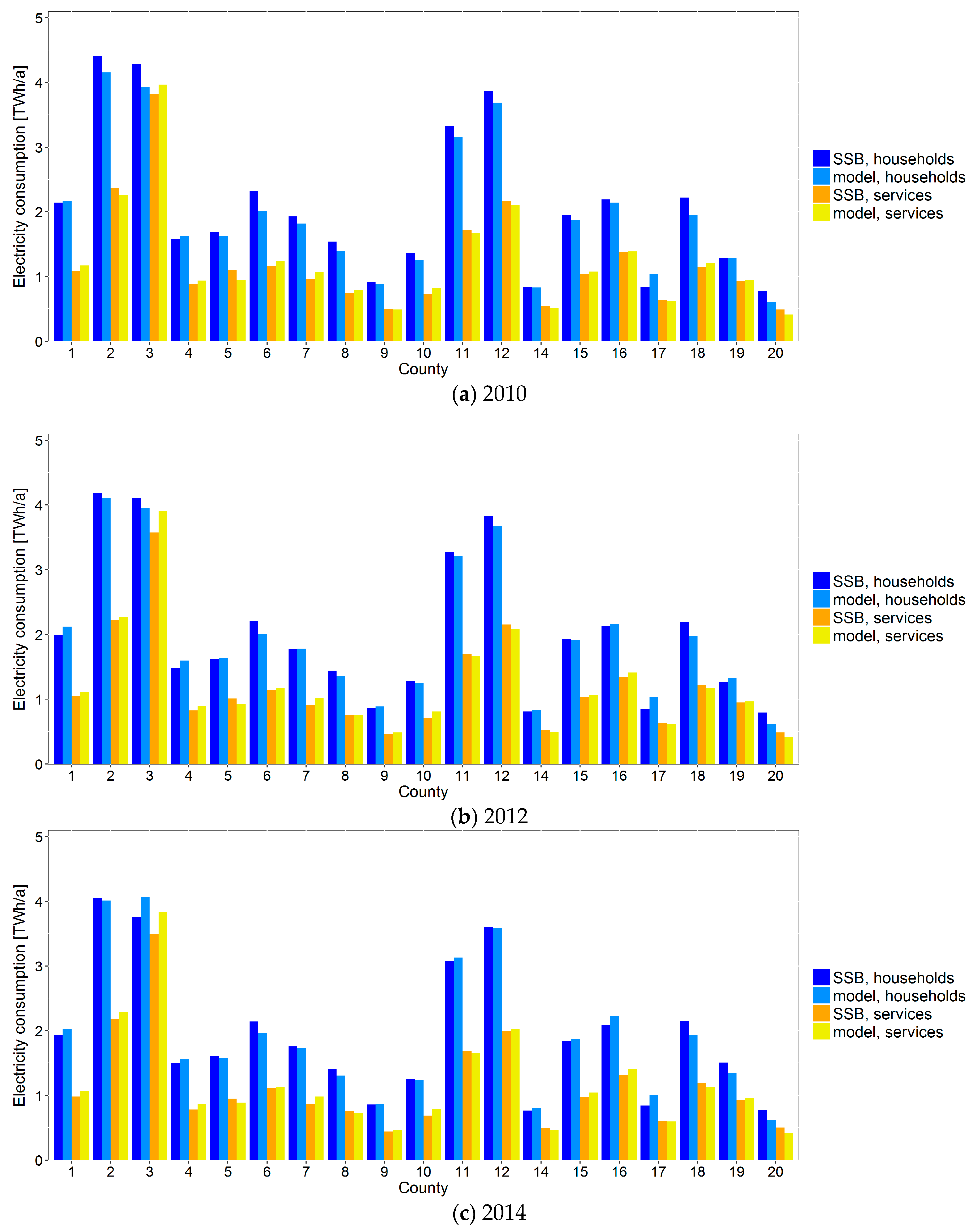
In order to validate our models, we first compare modeled and metered annual electricity consumption in households and services in each county in 2010, 2012 and 2014 (Figure 7). Metered consumption is provided by Statistics Norway (SSB) [45,46]. 2010 was an unusually cold year, 2012 a rather normal year, and 2014 an unusually warm year, with temperatures considerably above average during summer and winter.
For most counties, electricity consumption in both sectors in all three years is modeled with relative errors of less than 15%. However, in 2010 and 2012, consumption in the household sector is overestimated by more than 20% in county 17, which can be explained by different space heating habits (e.g., more intensive wood burning than assumed). In county 20, an especially cold region, household consumption is underestimated by more than 20%, which might also be due to poor assumptions regarding space heating systems, or by an insufficient estimation of HDD (e.g., by not choosing representative weather stations). Deviations between modeled and metered consumption in the service sector can partially be explained by the large uncertainty regarding the category others, which includes hotels and catering, culture, and all other service branches for which we do not have appropriate consumption models. Moreover, assumptions made on the share of non-residential buildings with non-electric heating might be insufficient.
4.2. Hourly Electricity Consumption per Sector and Nord Pool Region
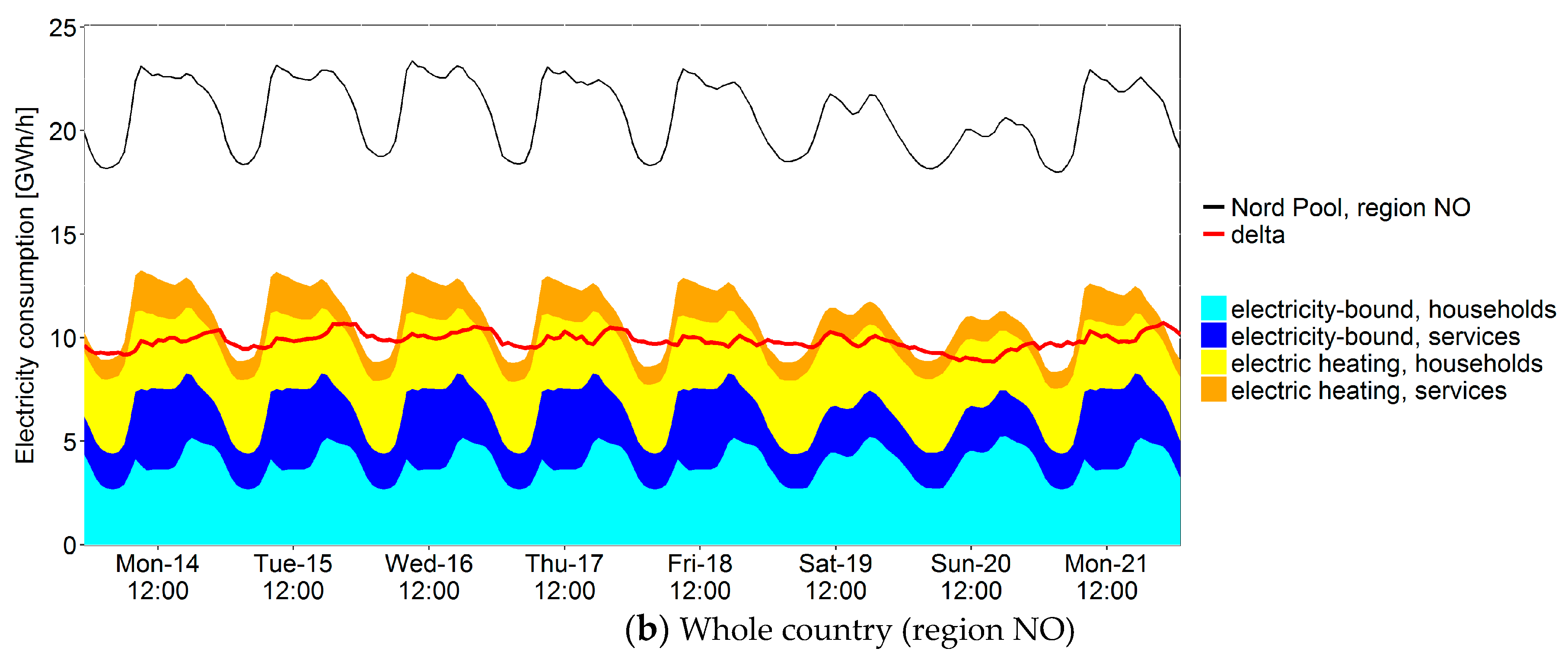
In a second step, we compare modeled hourly electricity consumption with hourly consumption data from Nord Pool, the Nordic power market [47] (Figure 8). Nord Pool divides Norway (NO) into five regions, called NO1 through NO5. Region NO1 approximately spans counties 1–6 and exhibits the highest consumption among the five regions. During a week in January in 2013, aggregate modeled consumption both for region NO1 (Figure 8a) and for the whole country NO (Figure 8b) fits the shape of metered consumption relatively well. The difference between metered and modeled consumption is called delta in the following and in theory represents electricity consumption in agriculture, industries, construction, and transport, as well as the modeling error. During the depicted time period, delta (red line) exhibits relatively small hourly variations, excepting slightly higher consumption during evening and nighttime, and slightly lower consumption during midday and on Sundays, which can be explained by reduced production in the industrial sector. As mentioned in Section 2.2, estimated electricity-bound consumption includes energy consumption for domestic water heating, while modeled consumption for electric heating only refers to space heating.
Average hourly electricity consumption in Norway (NO) on workdays in different months in 2013 is shown in Figure 9. Both during the colder months (January, February, and March) and the warmer months (May, June, and July), average modeled and metered hourly consumptions are similarly shaped, and the resulting average deltas are relatively constant over the course of the day. While during winter delta is approximately 9 GWh/h, it is only about 7GWh/h during summer. Thus, in theory, assuming that no consumers included in residual consumption delta (e.g., factories) shut down or use space cooling during summer, roughly about one fifth of delta were on average used for space heating purposes in January 2013.
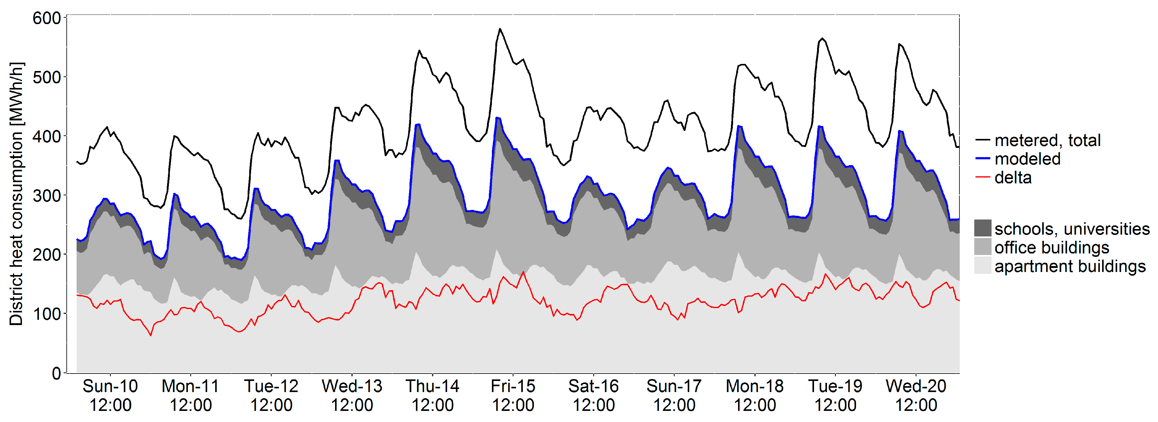
4.3. Case Study of Hourly District Heat Consumption in Oslo
Applying the same modeling approach as for electricity consumption, aggregate hourly consumption of district heat in different consumer groups can be modeled. A comparison of aggregate metered district heat consumption of all customers with hourly metering, supplied by Oslo’s largest district heat producer (black line), and aggregate modeled district heat consumption in office buildings, apartment buildings, and schools and universities (blue line) is shown in Figure 10. Obviously, the three consumer groups account for a large share of total (hourly metered) consumption; moreover, the hourly variations of modeled and metered district heat consumption are similar. The resulting difference delta (red line), representing other consumer groups such as industries and trade as well as the modeling error, is lowest during nighttime and highest during daytime, which can be explained by corresponding working hours, and thus seems feasible.
5. Discussion
5.1. Modeling Approach
In this study, regional aggregate hourly energy consumption is estimated based on regression models for hourly energy consumption of individual consumers. The method is simple and easy to replicate with corresponding training data; however, it has some drawbacks.
The applied household model is based on a sample which mainly consists of data connected to detached houses located in one specific county, while other dwelling types are poorly represented. For counties like Oslo, where apartments are the predominant dwelling type, the household model results are assumed to be less accurate than for a region with mainly detached houses. Moreover, energy-related building standards are only considered very roughly by including the dummy variable new—indicating whether the dwelling was built in 2000 or later. In order to use the models for forecasting, different energy standards, including, e.g., passive houses, should be taken into account.
The regression models for different building categories within the service sector are based on a relatively small sample of buildings, all located in Oslo, and floor space is the only cross-sectional variable. In some building categories, there were very few observations with non-electric heating so that only one regression model each, for all buildings within these categories, independent of heating system, could be developed. Moreover, mixed heating systems, e.g., combined electric and district heating, or the use of heat pumps, are not considered in the models, and the model for category others merges three building categories that might exhibit quite different hourly consumption profiles. Although there is an error connected to category others, we suppose it is useful to include it in order to model aggregate electricity consumption in the entire service sector.
Electricity consumption in dwellings and some non-residential building categories using non-electric heating is modeled by setting the HDD-dependent consumption to zero. Since modeled electricity-bound (HDD-independent) consumption in households usually includes some heat consumption that is less dependent on outdoor temperatures, e.g., for electric water heating or electric floor heating in bathrooms, modeled electricity consumption in households with non-electric heating might be slightly overestimated. Since, however, electric water heaters and electric floor heating are in fact broadly used, also in households with mainly non-electric space heating, we assume the method to be useful in order to make simple estimations.
In general, using mean floor space values in order to estimate consumption of average consumers (i.e., buildings) in each category, then multiplying these consumption values by the number of consumers in each category, generates uncertain results. Since all service sector models are exclusively based on panel data related to buildings located in Oslo, modeled consumption for all other counties is scaled using an arbitrarily defined factor, aiming to correct for differences in average number of employees per building. This scaling factor merely represents a “necessary evil” needed to obtain some simple estimates. With available panel data from different counties, more accurate models could be developed.
5.2. Uncertainties Regarding Input Data and Model Validation
A number of statistics on different household and dwelling characteristics, often on a county level, is provided by official statistics so that relatively detailed input data are available for modeling historic electricity consumption in the household sector. However, the shares of households using electric and non-electric heating, heat pumps, or wood stoves in each county are unknown so that the corresponding input data are based on assumptions, leading to increased uncertainty.
Official statistics on non-residential buildings in Norway are limited. While information on the absolute number of buildings per category and county is available, information on important factors such as floor space, year of construction, or energy carriers and heating systems used in each county is not. Thus, important input data for modeling aggregate electricity consumption in the service sector are missing and need to be substituted by assumptions. In order to make forecasts on regional aggregate consumption of different energy carriers more reliable input data for each region is crucial.
Hourly electricity consumption data per Nord Pool region does not allow for a proper validation of modeled aggregate hourly electricity consumption on county-level. Moreover, since we to date only have models for household and service sectors, the difference between metered and modeled consumption (delta) does not represent the modeling error alone, but also includes consumption in all other sectors, which prevents a thorough model validation.
5.3. Further Suggested Improvements
Base temperature tb varies across consumers and is not only dependent on the buildings’ energy standards but also on occupant behavior and individual preferences (e.g., regarding indoor temperature and thermostat usage). As the building stock is renewed, average base temperatures are expected to change for both residential and non-residential buildings; as such, the definitions of HDD and CDD possibly need to be adapted when using the models for forecasting. With corresponding meter data, the impact of different cross-sectional or further weather-related factors (e.g., wind or solar radiation) on tb could be examined in order to obtain estimates of current and future base temperatures that are useful for different consumer groups or building categories.
In Norway, space cooling is nowadays mainly used in non-residential buildings, however, as climate change is expected to lead to—on average—higher outdoor temperatures, space cooling is expected to become more important in residential buildings as well. Thus, in order to be used for forecasting regional energy consumption, our models should ideally incorporate space cooling in different building categories.
Charging of electric vehicles is assumed to be another important factor for modeling electricity consumption connected to a regional building stock, which is not yet implemented in our models, but could be incorporated with corresponding panel data.
Population increase and economic development, as well as the corresponding impacts on number and size of buildings and dwellings in each region, are key factors for future energy use. Increased energy efficiency of electric appliances, future building codes with respect to energy consumption, demolition or rehabilitation of older buildings, and construction rates of new buildings in each region are further factors that need to be considered when using the presented modeling approach for scenario analyses and forecasting.
6. Conclusions
In this study, regression models for hourly electricity consumption in individual dwellings and non-residential buildings are developed, and modeled consumption is divided into electricity-bound and space heating consumption. Aggregate regional hourly electricity consumption in households and service sectors in each Norwegian county is estimated by using average characteristics and total number of buildings or dwellings as input data to the models, and model validation indicates that this simple method in general is useful. However, larger relative errors of modeled annual electricity consumption in some counties indicate that more detailed input data (e.g., on heating systems used in each county) are desirable, and that models based on training data from only one region are not necessarily applicable to other regions. The overall shape of total aggregate hourly electricity consumption in Southeast Norway and in Norway as a whole is reproduced well by the models, indicating that mainly household and service sectors cause hourly variations in total regional electricity consumption. The same method was applied to model aggregate hourly district heat consumption of three consumer categories in Oslo, and a comparison with total metered consumption shows that the hourly variations are reproduced well, indicating that the method can also be useful for modeling aggregate hourly district heat consumption.
Sufficiently large training datasets containing meter data and cross-sectional variables connected to different building categories in different regions could considerably improve the individual models and, combined with more detailed input data for each region, yield more reliable results on modeled aggregate energy consumption.
More detailed hourly meter data of aggregate energy consumption, e.g., for each county and each economic sector, provided by utilities or system operators, would enable a more sophisticated model validation.
Well-maintained building stock databases and detailed surveys among different consumer groups in different regions could yield important cross-sectional data both for developing individual models and for generating input data for modeling and forecasting aggregate energy consumption on a regional level. Important factors such as the buildings’ energy and insulation standards, charging of electric vehicles, and energy efficiency of electric appliances and heating systems, need to be implemented in improved and more detailed models used for scenario analyses and forecasts. Furthermore, the improved models could be used for evaluating impacts of policy measures, like new building codes, energy taxes, and technological changes. Access to cross-sectional building information and sufficiently resolved meter data (including reliable links between those two data sources) are vital for model approaches similar to the one used in this study. With corresponding panel data on hand, the presented method can be applied to other countries, energy carriers, and temporal resolutions.
Acknowledgments
The study is partly funded by the Faculty of Environmental Sciences and Natural Resource Management, Norwegian University of Life Sciences, and partly by Energy Norway, through the Flexelterm project (www.flexelterm.no), with co-funding from The Norwegian Research Council under project No. 226260.
Author Contributions
The research of the statistical data, model development, results analysis and draft of the first version of the manuscript were done by Anna Kipping. Erik Trømborg contributed in defining objectives and framework of the paper, literature review, discussion and revisions.
Conflicts of Interest
The authors declare no conflict of interest.
Appendix A. Explanatory Variables

Table A1.
Explanatory variables, model for hourly electricity consumption in households.
| Variable | Symbol/Description | Type | Reference Group |
|---|---|---|---|
| x1 | dwelling group = attached | dummy | dwelling group = detached |
| x2,…,4 | number of adults = 2, 3, >3 | dummy | adults = 1 |
| x5,…,7 | number of children (<16 years) = 1, 2, >2 | dummy | children = 0 |
| x8 | senior resident = yes × (daytype = workday) | dummy | senior resident = no |
| x9 | (resident more than 20 h at home = yes) (daytype = workday) | dummy | resident more than 20 h at home = no |
| x10 | weekend resident = yes × (daytype = workday) | dummy | weekend resident = no |
| x11,…,13 | daytype = Saturday but no holiday, Sunday or holiday, workday within school-holidays | dummy | daytype = workday |
| x14 | cold storage = yes | dummy | cold storage = no |
| x15 | other electricity-intensive appliances = yes | dummy | appliances = no |
| x16,…,24 | month = 2, 3, 4, 5, 8, 9, 10, 11, 12 | dummy | month = 1 (January) |
| x25 | HDD | continuous | - |
| x26 | HDD1st | continuous | - |
| x27 | HDD × floor space | continuous | - |
| x28 | HDD × (dwelling group = attached) | cont./dummy | dwelling group = detached |
| x29 | HDD × (heat pump = yes) | cont./dummy | heat pump = no |
| x30 | HDD × (central electric boiler = yes) | cont./dummy | central electric boiler = no |
| x31 | HDD × (central heat pump = yes) | cont./dummy | central heat pump = no |
| x32 | HDD × (age = ≥2000) | cont./dummy | age = <2000 |
| x33 | HDD × (wood burning = supplementary) | cont./dummy | wood burning = no or only for coziness |
| x34 | HDD × (wood burning = mainly) | cont./dummy | wood burning = no or only for coziness |
Table A2.
Description of explanatory variables in service sector models.
| Variable | Symbol | Description | Type | Reference Group |
|---|---|---|---|---|
| x1 | A | average floor space | continuous | - |
| x2 | HDD | heating degree day | continuous | - |
| x3 | HDD1st | 1st differences in HDD | continuous | - |
| x4 | CDD | cooling degree day | continuous | - |
| x5,…,15 | month | month = 2, …, 12 | dummy | month = 1 (January) |
| x16 | free | d is a non-workday day | dummy | free = no |
| x17 | Sat | d is a Saturday but no holiday | dummy | Sat = no |
| x18 | Sun | d is a Sunday or holiday | dummy | Sun = no |
| x19 | school-holidays | d is within school-holidays, but not weekend or holiday | dummy | school-holidays = no |
Table A3.
Explanatory variables, service sector models, hourly electricity consumption.
| Variable | Offices, el. | Offices, Non-el. | Schools, el. | Schools, Non-el. | Kinder-Gartens | Shops | Health | Others |
|---|---|---|---|---|---|---|---|---|
| A | x | x | x | x | x | x | x | x |
| HDD | x | - | x | - | x | x | x | x |
| HDD1st | x | - | x | - | x | x | x | x |
| month | - | x | - | - | - | - | - | - |
| free | x | x | x | x | x | - | - | - |
| school-holidays | - | - | x | x | x | - | - | - |
| Sat | - | - | - | - | - | x | - | - |
| Sun | - | - | - | - | - | x | - | - |
| A × month | x | - | x | x | x | x | x | x |
| A × free | x | x | x | x | x | - | x | x |
| A × school-holidays | x | x | - | - | - | - | - | - |
| A × HDD | x | - | x | - | x | x | x | x |
| A × Sat | - | - | - | - | - | x | - | - |
| A × Sun | - | - | - | - | - | x | - | - |
| A × HDD × free | x | - | x | - | x | - | - | - |
| A × CDD × free | x | x | - | - | - | - | - | - |
| A × HDD × Sun | - | - | - | - | - | x | - | - |
| A × CDD × Sun | - | - | - | - | - | x | - | - |
Table A4.
Explanatory variables, models for hourly district heat consumption.
| Variable | Offices | Schools | Apartment Buildings |
|---|---|---|---|
| A | x | x | - |
| HDD | x | x | - |
| HDD1st | x | x | - |
| A × old | x | x | - |
| A × month | x | x | - |
| A × HDD | x | x | x |
| A × HDD1st | - | - | x |
| A × HDD·old | x | x | - |
| A × HDD·free | x | x | - |
| A × HDD × school-holidays | x | x | - |
| apartments | - | - | x |
| apartments·free | - | - | x |
| apartments·month | - | - | x |
References
- Statistics Norway (SSB), Energy Balance, Table 11561. Available online: https://www.ssb.no/statistikkbanken/selectvarval/Define.asp?subjectcode=&ProductId=&MainTable=EnergiBalanse2&nvl=&PLanguage=0&nyTmpVar=true&CMSSubjectArea=energi-og-industri&KortNavnWeb=energibalanse&StatVariant=&checked=true (accessed on 18 November 2017).
- Bøeng, A.C.; Holstad, M. Fakta om Energi—Utviklingen i Energibruk i Norge. Available online: https://www.ssb.no/energi-og-industri/artikler-og-publikasjoner/_attachment/104473?_ts=13d86acd6f8 (accessed on 28 December 2017).
- Statistics Norway (SSB), Energy Balance, Table 08311. Available online: https://www.ssb.no/statistikkbanken/selectvarval/Define.asp?subjectcode=&ProductId=&MainTable=NtoForbKraftGrupp&nvl=&PLanguage=1&nyTmpVar=true&CMSSubjectArea=energi-og-industri&KortNavnWeb=elektrisitet&StatVariant=&checked=true (accessed on 15 December 2017).
- Statistics Norway (SSB), Energy Accounting, Table 04372. Available online: https://www.ssb.no/statistikkbanken/selectvarval/Define.asp?subjectcode=&ProductId=&MainTable=AndreFormal&nvl=&PLanguage=0&nyTmpVar=true&CMSSubjectArea=energi-og-industri&KortNavnWeb=energiregnskap&StatVariant=&checked=true (accessed on 15 December 2017).
- Statistics Norway (SSB). Share of Heating Equipment Used, Per Dwelling Type, Table 10568. Available online: https://www.ssb.no/statistikkbanken/selectvarval/Define.asp?subjectcode=&ProductId=&MainTable=HusenVarmutstyr&nvl=&PLanguage=1&nyTmpVar=true&CMSSubjectArea=energi-og-industri&KortNavnWeb=husenergi&StatVariant=&checked=true (accessed on 15 December 2017).
- Rosenberg, E.; Lind, A.; Espegren, K.A. The impact of future energy demand on renewable energy production—Case of Norway. Energy 2013, 61, 419–431. [Google Scholar] [CrossRef]
- Seljom, P.; Rosenberg, E.; Fidje, A.; Haugen, J.E.; Meir, M.; Rekstad, J.; Jarlset, T. Modelling the effects of climate change on the energy system—A case study of Norway. Energy Policy 2011, 39, 7310–7321. [Google Scholar] [CrossRef]
- Andersen, F.; Larsen, H.; Boomsma, T. Long-term forecasting of hourly electricity load: Identification of consumption profiles and segmentation of customers. Energy Convers. Manag. 2013, 68, 244–252. [Google Scholar] [CrossRef]
- Andersen, F.; Larsen, H.; Gaardestrup, R. Long term forecasting of hourly electricity consumption in local areas in Denmark. Appl. Energy 2013, 110, 147–162. [Google Scholar] [CrossRef]
- Swan, L.G.; Ugursal, V.I. Modeling of end-use energy consumption in the residential sector: A review of modeling techniques. Renew. Sustain. Energy Rev. 2009, 13, 1819–1835. [Google Scholar] [CrossRef]
- Kavgic, M.; Mavrogianni, A.; Mumovic, D.; Summerfield, A.; Stevanovic, Z.; Djurovic-Petrovic, M. A review of bottom-up building stock models for energy consumption in the residential sector. Build. Environ. 2010, 45, 1683–1697. [Google Scholar] [CrossRef]
- Richardson, I.; Thomson, M.; Infield, D.; Clifford, C. Domestic electricity use: A high-resolution energy demand model. Energy Build. 2010, 42, 1878–1887. [Google Scholar] [CrossRef] [Green Version]
- Yao, R.; Steemers, K. A method of formulating energy load profile for domestic buildings in the UK. Energy Build. 2005, 37, 663–671. [Google Scholar] [CrossRef]
- McLoughlin, F.; Duffy, A.; Conlon, M. Characterising domestic electricity consumption patterns by dwelling and occupant socio-economic variables: An Irish case study. Energy Build. 2012, 48, 240–248. [Google Scholar] [CrossRef]
- Widén, J.; Wäckelgård, E. A high-resolution stochastic model of domestic activity patterns and electricity demand. Appl. Energy 2010, 87, 1880–1892. [Google Scholar] [CrossRef]
- Foucquier, A.; Robert, S.; Suard, F.; Stéphan, L.; Jay, A. State of the art in building modelling and energy performances prediction: A review. Renew. Sustain. Energy Rev. 2013, 23, 272–288. [Google Scholar] [CrossRef]
- Brøgger, M.; Wittchen, K. Estimating the energy-saving potential in national building stocks—A methodology review. Renew. Sustain. Energy Rev. 2018, 82, 1489–1496. [Google Scholar] [CrossRef]
- Aydinalp, M.; Ugursal, V.I.; Fung, A.S. Modeling of the appliance, lighting, and space-cooling energy consumptions in the residential sector using neural networks. Appl. Energy 2002, 71, 87–110. [Google Scholar] [CrossRef]
- Aydinalp, M.; Ugursal, V.I.; Fung, A.S. Modeling of the space and domestic hot-water heating energy-consumption in the residential sector using neural networks. Appl. Energy 2004, 79, 159–178. [Google Scholar] [CrossRef]
- Beccali, M.; Cellura, M.; Brano, V.L.; Marvuglia, A. Forecasting daily urban electric load profiles using artificial neural networks. Energy Convers. Manag. 2004, 45, 2879–2900. [Google Scholar] [CrossRef]
- Beccali, M.; Cellura, M.; Brano, V.L.; Marvuglia, A. Short-term prediction of household electricity consumption: Assessing weather sensitivity in a mediterranean area. Renew. Sustain. Energy Rev. 2008, 12, 2040–2065. [Google Scholar] [CrossRef]
- Rodrigues, F.; Cardeira, C.; Calado, J. The daily and hourly energy consumption and load forecasting using artificial neural network method: A case study using a set of 93 households in Portugal. Energy Procedia 2014, 62, 220–229. [Google Scholar] [CrossRef]
- Chae, Y.T.; Horesh, R.; Hwang, Y.; Lee, Y.M. Artificial neural network model for forecasting sub-hourly electricity usage in commercial buildings. Energy Build. 2016, 111, 184–194. [Google Scholar] [CrossRef]
- Magalhães, S.; Leal, V.; Horta, I. Modelling the relationship between heating energy use and indoor temperatures in residential buildings through Artificial Neural Networks considering occupant behavior. Energy Build. 2017, 151, 332–343. [Google Scholar] [CrossRef]
- Fels, M.F. PRISM: An introduction. Energy Build. 1986, 9, 5–18. [Google Scholar] [CrossRef]
- Pedersen, L.; Stang, J.; Ulseth, R. Load prediction method for heat and electricity demand in buildings for the purpose of planning for mixed energy distribution systems. Energy Build. 2008, 40, 1124–1134. [Google Scholar] [CrossRef]
- Braun, M.; Altan, H.; Beck, S. Using regression analysis to predict the future energy consumption of a supermarket in the UK. Appl. Energy 2014, 130, 305–313. [Google Scholar] [CrossRef]
- Amiri, S.; Mottahedi, M.; Asadi, S. Using multiple regression analysis to develop energy consumption indicators for commercial buildings in the U.S. Energy Build. 2015, 109, 209–216. [Google Scholar] [CrossRef]
- Fumo, N.; Biswas, M.R. Regression analysis for prediction of residential energy consumption. Renew. Sustain. Energy Rev. 2015, 47, 332–343. [Google Scholar] [CrossRef]
- Pulido-Arcas, J.; Pérez-Fargallo, A.; Rubio-Bellido, C. Multivariable regression analysis to assess energy consumption and CO2 emissions in the early stages of offices design in Chile. Energy Build. 2016, 133, 738–753. [Google Scholar] [CrossRef]
- Oh, S.; Ng, K.; Thu, K.; Chun, W.; Chua, K. Forecasting long-term electricity demand for cooling of Singapore’s buildings incorporating an innovative air-conditioning technology. Energy Build. 2016, 127, 183–193. [Google Scholar] [CrossRef]
- Arregi, B.; Garay, R. Regression analysis of the energy consumption of tertiary buildings. Energy Procedia 2017, 122, 9–14. [Google Scholar] [CrossRef]
- Wang, L.; Kubichek, R.; Zhou, X. Adaptive learning based data-driven models for predicting hourly building energy use. Energy Build. 2018, 159, 454–461. [Google Scholar] [CrossRef]
- Kipping, A.; Trømborg, E. Hourly electricity consumption in norwegian households—Assessing the impacts of different heating systems. Energy 2015, 93 Pt 1, 655–671. [Google Scholar] [CrossRef]
- Kipping, A.; Trømborg, E. Modeling and disaggregating hourly electricity consumption in Norwegian dwellings based on smart meter data. Energy Build. 2016, 118, 350–369. [Google Scholar] [CrossRef]
- Kipping, A.; Trømborg, E. Modeling hourly consumption of electricity and district heat in non-residential buildings. Energy 2017, 123, 473–486. [Google Scholar] [CrossRef]
- Statistics Norway (SSB). Dwelling Types and Floor Space, Table 06513. Available online: https://www.ssb.no/statistikkbanken/SelectVarVal/define.asp?SubjectCode=al&ProductId=al&MainTable=BoligBygnBruks&contents=Boliger5&PLanguage=0&Qid=0&nvl=True&mt=1&pm=&SessID=8116073&FokusertBoks=1&gruppe1=Hele&gruppe2=Hele&gruppe3=Hele&gruppe4=Hele&VS1=Fylker&VS2=Bygninger06&VS3=Bruksareal7&VS4=&CMSSubjectArea=&KortNavnWeb=boligstat&StatVariant=&Tabstrip=SELECT&aggresetnr=1&checked=true (accessed on 26 July 2016).
- Statistics Norway (SSB). Table 06266: Dwellings, by Type of Building and Year of Construction. Available online: https://www.ssb.no/statistikkbanken/SelectVarVal/define.asp?SubjectCode=al& ProductId=al&MainTable=BoligerB&contents=Boliger&PLanguage=0&Qid=0&nvl=True&mt=1& pm=&SessID=8353112&FokusertBoks=1&gruppe1=Hele&gruppe2=Hele&gruppe3=Hele&gruppe4=Hele&VS1=Fylker&VS2=Bygninger05&VS3=BygnAr&VS4=&CMSSubjectArea=&KortNavnWeb=boligstat&StatVariant=&Tabstrip=SELECT&aggresetnr=1&checked=true (accessed on 24 August 2016).
- Statistics Norway (SSB). Population, Table 06913. Available online: https://www.ssb.no/statistikkbanken/SelectVarVal/Define.asp?MainTable=Folkemengd1951&KortNavnWeb=folkemengde& PLanguage=0&checked=true (accessed on 26 July 2016).
- Statistics Norway (SSB). Population and Housing Census, Table 09810. Available online: https://www.ssb.no/statistikkbanken/SelectVarVal/Define.asp?MainTable=FOBbolAldBAarByg&KortNavnWeb= fobbolig&PLanguage=0&checked=true (accessed on 26 July 2016).
- Statistics Norway (SSB). Families and Households, Table 10986. Available online: https://www.ssb.no/statistikkbanken/SelectVarVal/define.asp?SubjectCode=al&ProductId=al&MainTable=HushTypRegion&contents=Personer&PLanguage=0&Qid=0&nvl=True&mt=1&pm=&SessID=8073068&FokusertBoks=2&gruppe1=Hele&gruppe2=Hele&gruppe3=Hele&VS1=FylkerFastland&VS2=HusholdType2006niv2&VS3=&CMSSubjectArea=&KortNavnWeb=familie&StatVariant=&Tabstrip=SELECT&aggresetnr=2&checked=true (accessed on 26 July 2016).
- Statistics Norway (SSB). Employment, Table 09315. Available online: https://www.ssb.no/statistikkbanken/SelectVarVal/Define.asp?MainTable=SysselAldNar&KortNavnWeb=regsys&PLanguage=0& checked=true (accessed on 26 July 2016).
- Statistics Norway (SSB). Number of Buildings per County and Building Type 2006–2016. Available online: https://www.ssb.no/en/bygg-bolig-og-eiendom/statistikker/byggeareal/aar/2016-02-15?fane=tabell#content (accessed on 30 March 2016).
- Norwegian Energy Labels for Buildings. Available online: http://www.energimerking.no/ (accessed on 1 August 2016).
- Statistics Norway (SSB). Electricity Consumption in the Service Sector per Category and County. Available online: http://ec.europa.eu/eurostat/statistics-explained/index.php/Electricity_and_heat_statistics (accessed on 19 May 2016).
- Statistics Norway (SSB). Electricity, Annual Figures per Consumer Group and Region, 2011–2014, Table 10314. Available online: https://www.ssb.no/statistikkbanken/SelectVarVal/Define.asp?MainTable=NtoForbKraftGrKom&KortNavnWeb=elektrisitet&PLanguage=0&checked=true (accessed on 1 August 2016).
- Hourly Electricity Consumption Data. Available online: http://www.nordpoolspot.com/historical-market-data/ (accessed on 15 August 2016).
- Hourly Meter Data of Aggregate District Heat Consumption in Oslo. Available online: https://www.gov.uk/government/uploads/system/uploads/attachment_data/file/267585/Sub-national_electricity_consumption_factsheet_2012.pdf (accessed on 8 March 2017).
Figure 1.
Total energy consumption (excluding transport and energy industries), per energy carrier, Norway, 1976–2015 [4].
Figure 1.
Total energy consumption (excluding transport and energy industries), per energy carrier, Norway, 1976–2015 [4].

Figure 2.
Electricity consumption, per sector, Norway, 1993–2016 [3].
Figure 2.
Electricity consumption, per sector, Norway, 1993–2016 [3].

Figure 3.
Modeling electricity-bound and space heating energy consumption.

Figure 4.
Modeling aggregate hourly electricity consumption in the household sector.

Figure 5.
Modeling aggregate hourly electricity consumption in different service sector categories.

Figure 6.
Adjustment factor f for each county and non-residential building category.

Figure 7.
Modeled and metered (SSB [45,46]) electricity consumption in household and service sectors per county, 2010, 2012 and 2014.

Figure 8.
Modeled electricity consumption in household and service sector, metered total consumption [47], and residual consumption delta, January 2013.
Figure 8.
Modeled electricity consumption in household and service sector, metered total consumption [47], and residual consumption delta, January 2013.
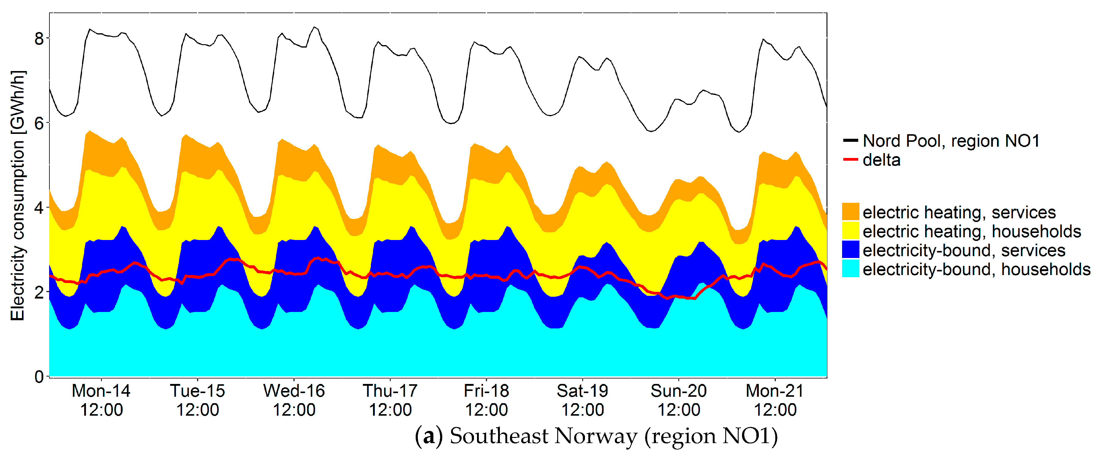

Figure 9.
Average hourly electricity consumption in different months (workdays), 2013, metered (Nord Pool, NO [47]), modeled, and residual consumption delta: (a) January, February, March, (b) May, June, July.
Figure 9.
Average hourly electricity consumption in different months (workdays), 2013, metered (Nord Pool, NO [47]), modeled, and residual consumption delta: (a) January, February, March, (b) May, June, July.
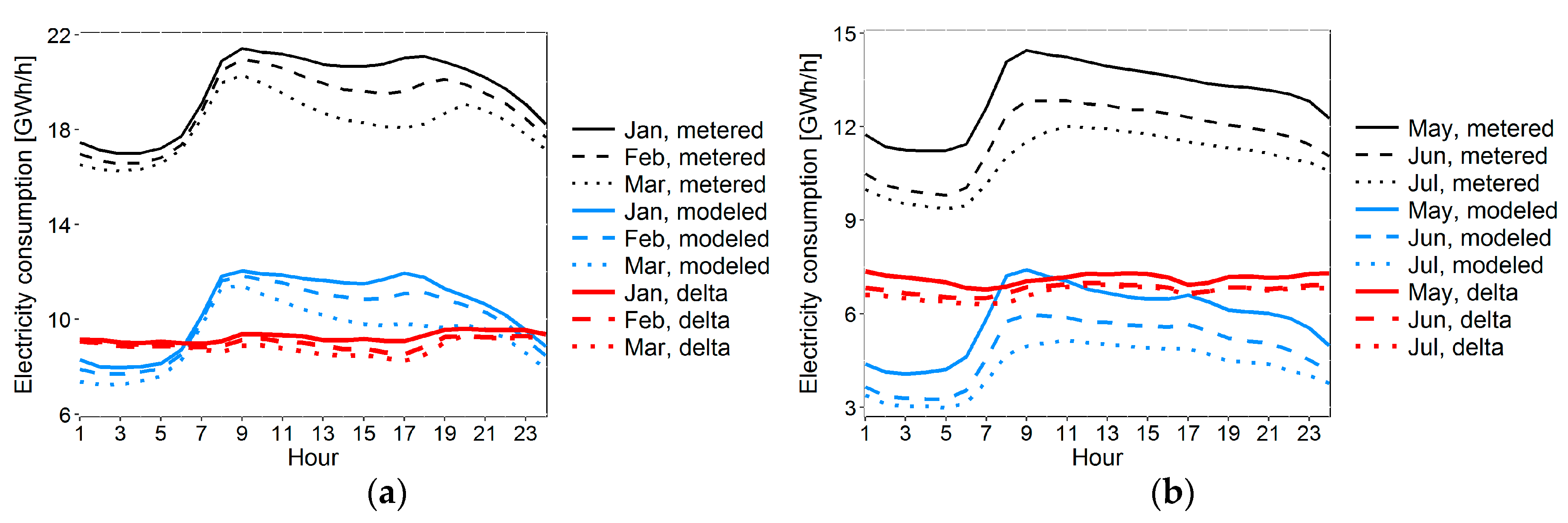
Figure 10.
Modeled and metered [48] district heat consumption, and residual consumption delta, January 2016.
Figure 10.
Modeled and metered [48] district heat consumption, and residual consumption delta, January 2016.

Table 1.
Model overview, hourly electricity consumption.
| Sector | Consumer Category | Building Category (Meter Data) | Separate Models for Electric/Non-Electric Heating | References |
|---|---|---|---|---|
| households | households | dwellings | no | [34,35] |
| services | offices | office buildings | yes | [36] |
| services | education | schools, universities | yes | [36] |
| services | education | kindergartens | no | - |
| services | trade | shops, stores | no | - |
| services | health | nursing homes | no | - |
| services | others | hotels, museums | no | - |
© 2017 by the authors. Licensee MDPI, Basel, Switzerland. This article is an open access article distributed under the terms and conditions of the Creative Commons Attribution (CC BY) license (http://creativecommons.org/licenses/by/4.0/).
Share and Cite
MDPI and ACS Style
Kipping, A.; Trømborg, E. Modeling Aggregate Hourly Energy Consumption in a Regional Building Stock. Energies 2018, 11, 78. https://doi.org/10.3390/en11010078
AMA Style
Kipping A, Trømborg E. Modeling Aggregate Hourly Energy Consumption in a Regional Building Stock. Energies. 2018; 11(1):78. https://doi.org/10.3390/en11010078
Chicago/Turabian StyleKipping, Anna, and Erik Trømborg. 2018. "Modeling Aggregate Hourly Energy Consumption in a Regional Building Stock" Energies 11, no. 1: 78. https://doi.org/10.3390/en11010078
Note that from the first issue of 2016, this journal uses article numbers instead of page numbers. See further details here.