Anisotropy in Thermal Recovery of Oil Shale—Part 1: Thermal Conductivity, Wave Velocity and Crack Propagation


Institute of Mining Technology, Taiyuan University of Technology, Taiyuan 030024, China
*
Author to whom correspondence should be addressed.
Energies 2018, 11(1), 77; https://doi.org/10.3390/en11010077
Submission received: 4 November 2017
/
Revised: 21 December 2017
/
Accepted: 22 December 2017
/
Published: 1 January 2018
Abstract
:In this paper, the evolution of thermal conductivity, wave velocity and microscopic crack propagation both parallel and perpendicular to the bedding plane in anisotropic rock oil shale were studied at temperatures ranging from room temperature to 600 °C. The results show that the thermal conductivity of the perpendicular to bedding direction (KPER) (PER: perpendicular to beeding direction), wave velocity of perpendicular to bedding diretion (VPER), thermal conduction coefficient of parallel to beeding direction (KPAR) and wave velocity of parallel to beeding direction (VPAR) (PAR: parallel to bedding direction) decreased with the increase in temperature, but the rates are different. KPER and VPER linearly decreased with increasing temperature from room temperature to 350 °C, with an obvious decrease at 400 °C corresponding to a large number of cracks generated along the bedding direction. KPER, VPER, KPAR and VPAR generally maintained fixed values from 500 °C to 600 °C. 400 °C has been identified as the threshold temperature for anisotropic evolution of oil shale thermal physics. In addition, the relationship between the thermal conductivity and wave velocity based on the anisotropy of oil shale was fitted using linear regression. The research in this paper can provide reference for the efficient thermal recovery of oil shale, thermal recovery of heavy oil reservoirs and the thermodynamic engineering in other sedimentary rocks.
1. Introduction
Oil shale is a fine-grained sedimentary rock that typically has a high ash content along with combustible organic matter. Its organic substance, also called kerogen, can be decomposed into oil shale oil and pyrolysis oil gas [1] at specific temperatures. Oil shale resources are abundant across the world and are often thought to be an important supplementary energy source. China’s oil shale reserves rank second in the world, equivalent to 476 tons of shale oil [2]. Exploitation of oil shale can be aboveground (ex situ) or underground (in situ). Because of the problems of high cost and high pollution, ex-situ retorting pyrolysis of oil shale has been gradually eliminated in recent years, and the method of in-situ direct pyrolysis of oil shale has been gradually replacing ex-situ pyrolysis. The current method of in-situ direct pyrolysis of oil shale mainly includes: Shell’s in-situ conversion process (ICP) (Figure 1a) [3], ExxonMobil’s Electrofrac technology [4], Chevron’s CRUSH technology [5] and China’s in-situ steam-injection technology implemented by Taiyuan University of Technology (Figure 1b) [6]. The basic principle behind all of these shale oil and gas exploitation methods is to bring some heat energy to oil shale formations, and when the oil shale formation reaches the pyrolysis temperature of kerogen, kerogen begins pyrolysis to transform into gaseous pyrolysis oil and gas. The oil and gas pyrolysis products migrate towards the production well and are pumped to the surface. Therefore, the key to mining oil shale is to increase the temperature of the oil shale layer to the pyrolysis temperature as soon as possible.
Oil shale, as a kind of sedimentary organic-rich rock, has a strong anisotropy in thermal conductivity, wave velocity and mechanic properties due to the alignment of anisotropic clay minerals and the parallel-bedding lamination of material within the shale [7,8]. If the anisotropy coefficient is greater than 1.5 [9], it will cause great error in engineering practices with the well and formation. Under the influence of temperature, the thermal conductivity, mechanical properties and permeability of oil shale drastically change along with its anisotropy. In order to better study the conduction process of temperature in oil shale, it is necessary to study the evolutionary process of thermal physical properties both in the vertical bedding direction and parallel bedding direction with temperature. If the anisotropy of temperature conduction in oil shale strata is neglected, the conduction range of temperature will be wrongly predicted, thus affecting the effective exploitation of the formation. The anisotropy of the conduction of the temperature also affects other thermodynamic engineering, such as the thermal recovery of heavy oil [10,11,12].
Several studies have described the variation in thermal conductivity of rock with temperature. Generally, thermal conductivity decreases with the increase in temperature [13,14]. Under increased temperatures, the change and loss of mineral composition inside the rock, the propagation of microcracks and the change in pore structure will decrease the thermal conductivity of the rock sample [15,16]. Different from other rocks, oil shale is more sensitive to increases in temperature with regards to its physical and mechanical properties. Under certain temperatures, the organic matter will be pyrolyzed, resulting in the increase of porosity and fracture development [17,18]. The increase of porosity and development of fissures change the low permeability of oil shale under normal temperatures [19]. From room temperature to 300 °C, the porosity of oil shale increases slowly, and the porosity dramatically increases at 400 °C. From then on, porosity increases slowly from 500 °C to 600 °C [17,18,20,21], indicating that the main pyrolysis temperature range of oil shale is between 400 °C and 500 °C, as observed by the thermo–gravimetric curve [22]. The decomposition of kerogen in oil shale increases the pressure in the rock, and abundant fissures are produced along the bedding plane of the oil shale, while only a small amount of fractures occur in the direction perpendicular to the bedding plane [23,24]. Temperature change has an important influence on the development of pores and fractures within oil shale, and the existence of pores and fissures has certainly affected the thermophysical properties, such as the thermal conductivity, of oil shale.
Although there have been many studies on the influence of temperature on the thermal conductivity of oil shale or other rocks, there are only a few studies on the influence of temperature on the anisotropy of thermal conductivity of rock. The anisotropy of rock can be divided into initial anisotropy and induced anisotropy, in which the anisotropy induced by anisotropic arrangement of minerals in rocks and along the bedding surface structure is called the initial anisotropy. The anisotropy induced by temperature, moisture content and stress is called the induced anisotropy [25], and temperature is one of the main causes of changes in anisotropy [26]. Many have studied the anisotropic thermal conductivity of rock under normal temperatures. Kim et al. [27] has studied the thermal conductivity of the Asan gneiss and Boryeong shale, finding that the ratio of KPAR (thermal conductivity of parallel to bedding planes) to KPER (thermal conductivity of perpendicular to bedding planes) is 1.4, and the anisotropy of thermal conductivity in the shale is obvious. The wave velocity in a rock is usually used as a physical parameter [28,29] to predict the elastic modulus and thermal conductivity of rock. It is also affected by changes in the material and fracture development, with the wave velocity tending to decrease with an increase in temperature. Therefore, relationships between thermal conductivity and wave velocity have been developed for different rock types. Some rocks have an exponential relationship between the wave velocity and heat transfer coefficient, such as limestone, while others are linear, such as the Boryeong shale [29]. However, most of the fitting relationships established are based on the assumption of rock isotropy, although rocks have a tendency to display anisotropic effects, particularly when heated.
There are several differences between this study and previous work on thermal conductivity, wave velocity and crack propagation within oil shale and other rocks. Previous studies on the anisotropy of heat conduction and wave velocity were primarily conducted at room temperature. Most of these studies also considered the effect of stress and water content on anisotropy, while seldom considering the effect of temperature on thermal conductivity and wave velocity. Also, previous studies on the influence of temperature on thermal conductivity and wave velocity were conducted on sandstone and granite, which can be regarded as homogeneous rocks. Few studies also considered the effect of temperature and anisotropy on thermal conductivity and wave velocity of these rocks. Therefore, this paper studies the reasons for the variation of thermal conductivity and wave velocity anisotropy coefficient of oil shale, analyzed by microscopic CT (Computed Tomography) test. Finally, most of the fitting relationships previously established are based on the assumption of rock isotropy. In this paper, the fitting relationship between the thermal conductivity and wave velocity considers anisotropy for a more accurate depiction of oil shale.
In this study, a series of procedures were designed to study the anisotropy of thermal conductivity, wave velocity and crack propagation at high temperature. Firstly, the thermal diffusivity at different temperatures was measured by a thermal conductivity analyzer. Then, the thermal conductivity of different temperatures was calculated according to the thermal diffusivity, and the influence of temperature on the thermal conductivity of different bedding directions was analyzed and is discussed. Secondly, the wave velocity of oil shale at different temperatures was measured by an ultrasonic rock parameter instrument, the influence of temperature on wave velocity is then discussed, and the relationship between the heat conduction coefficient and wave velocity obtained. Finally, the principles of crack propagation in oil shale under different temperatures was observed by micro CT, and the reason for the change of anisotropy coefficient of oil shale thermal conductivity and wave velocity is discussed.
2. Materials and Methods
2.1. Description of Oil Shale Samples
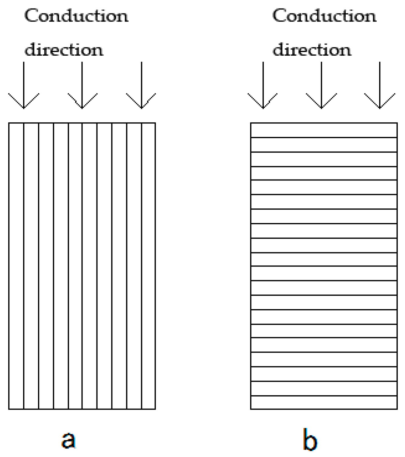
The selected oil shale samples are from the Liaoning Fushun open pit mine. The samples are dark black at room temperature with an average density of 2.2 g/cm3. To test the anisotropy of the shale, the longest part of the sample was either parallel or perpendicular to the bedding planes (Figure 2). The specific shape of each specimen is shown in Table 1.
2.2. Experimental Process
2.2.1. Thermal Conductivity Experiment
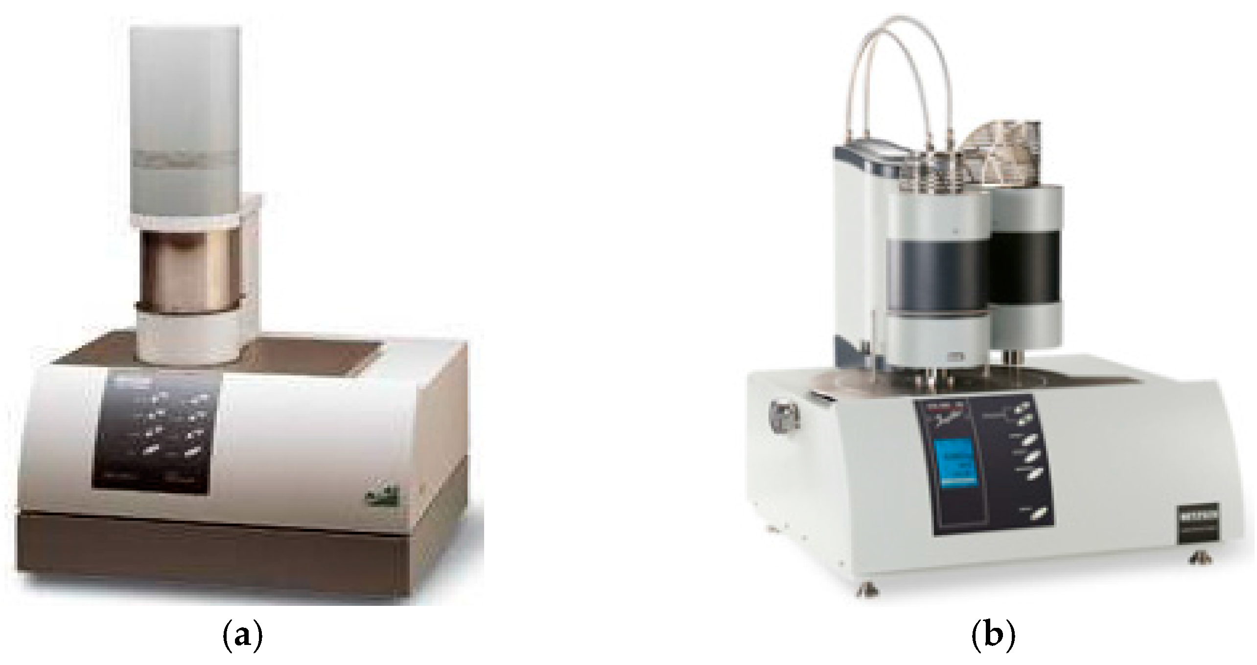
Thermogravimetric analysis of one oil shale sample was performed using an STA 449F3 (Netzsch, Selb, Germany), as shown in Figure 3a. The heating rate was 10 °C/min, with a maximum temperature of 600 °C under a nitrogen atmosphere that was maintained at flow rate of 50 mL∙min−1.
The thermal diffusivity of the samples was measured by a Netzsch LFA 457 laser thermal conductivity analyzer (Netzsch, Selb, Germany), as shown in Figure 3b. Firstly, the furnace body of the thermal conductivity instrument was raised to predetermined temperatures in order (100 °C, 200 °C, 300 °C, 350 °C, 400 °C, 450 °C, 500 °C, 550 °C, 600 °C), and argon gas was applied during heating. The rate of flow for the argon gas was 80 mL/min. Thermal diffusivity was measured three times at each temperature point to calculate an average value for a temperature.
2.2.2. Wave Velocity Test Experiment
Testing of the wave velocity of the oil shale samples was performed by the SYC-2 ultrasonic rock parameter instrument (Xiangtan wireless company, Xiangtan, China), as shown in Figure 3c. The accuracy of the instrument was 0.1 . The end face of the specimen was kept flat so as to have better contact with the transducers. The specimen was then put into a muffle furnace under a nitrogen atmosphere and heated to a specified temperature (100 °C, 200 °C, 300 °C, 350 °C, 400 °C, 450 °C, 500 °C, 550 °C, 600 °C). Once the sample reached the specified temperature, it was immediately removed from the furnace and the wave velocity was tested. Grease was applied between the specimen and probe during the test to increase the coupling between the specimen and transducers. After testing, the specimen was returned to the furnace and heated to the next specified temperature for wave velocity testing.
2.2.3. Crack Propagation Experiment
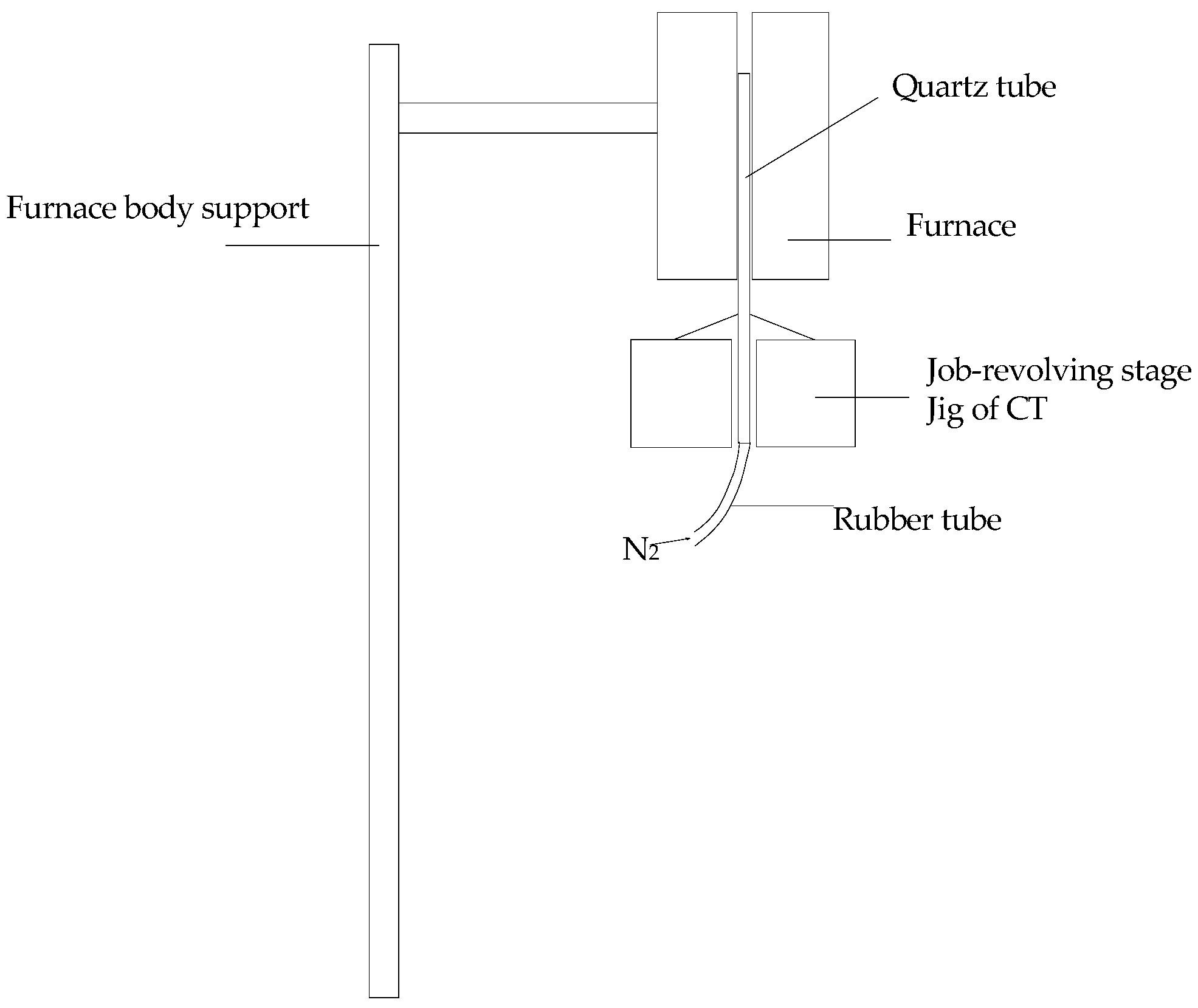
Crack propagation within oil shale under various temperatures was obtained by CT (Computed Tomography) equipment developed by Taiyuan University of Technology, as shown in Figure 3d. The position of the jig was adjusted so that the ray completely scanned the specimen while recording the location coordinates of the jig through the control system of the CT. The jig was then moved so that the quartz tube extended into the furnace, as shown in Figure 4. The specimen was heated to the intended temperature (100 °C, 200 °C, 300 °C, 350 °C, 400 °C, 450 °C, 500 °C, 550 °C, 600 °C) under a nitrogen atmosphere, the specimen was removed from the furnace and the jig was moved to the previous coordinate position to ensure that the specimen was scanned at the same position to monitor the propagation of cracks throughout the specimen. After the scanning was complete for a temperature, the sample was moved back into the heating furnace and heated to the next set temperature before being scanned again.
3. Results
3.1. Anisotropy of Thermal Conductivity
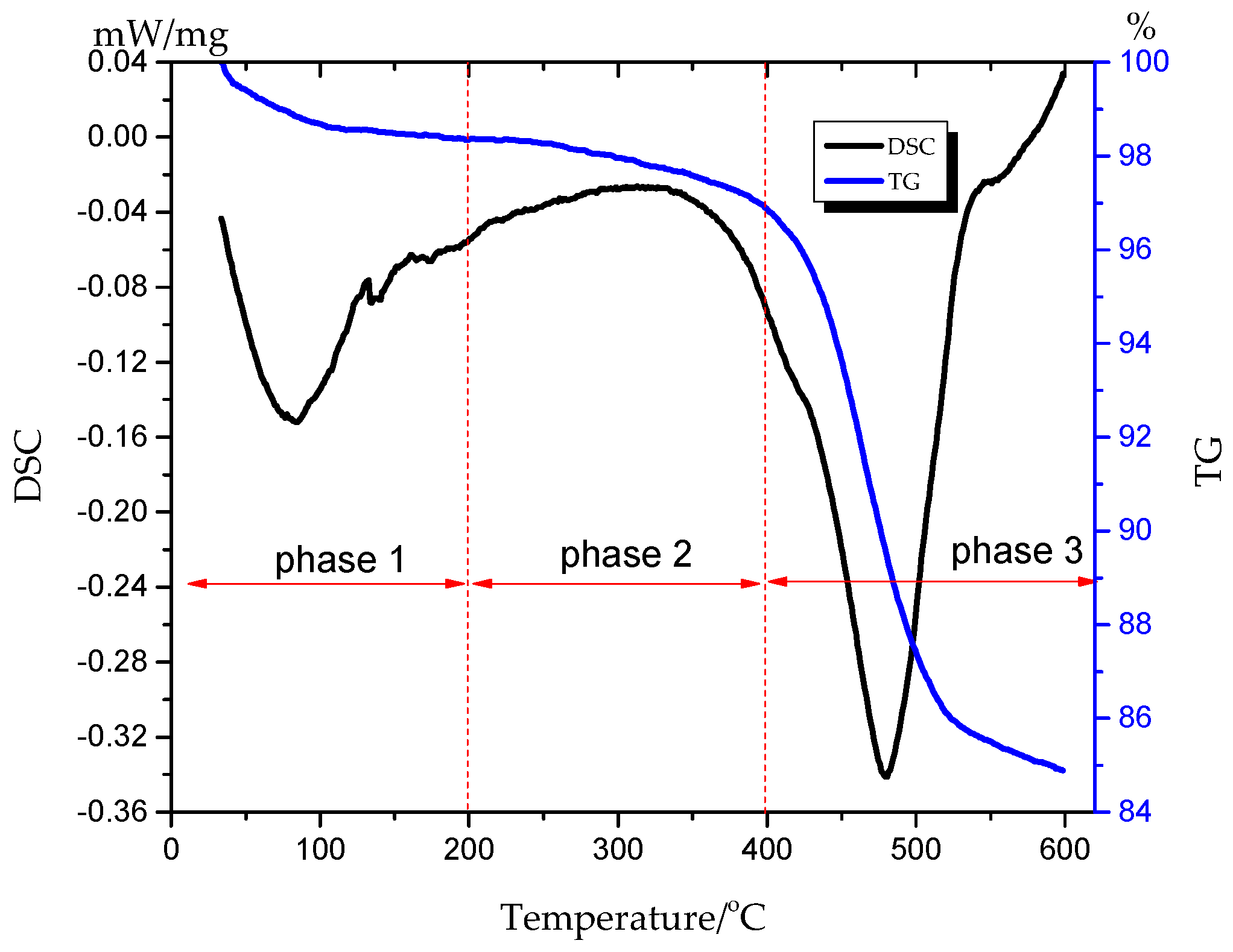
Figure 5 shows thermal analysis diagrams for differential scanning calorimetry (DSC) curves and thermogravimetric (TG) curves of the oil shale specimen. From the thermogravimetric (TG) curve, the weight loss stage of the oil shale can be divided into three phases: (1) from room temperature to 200 °C, the main loss of this phase was the free water and bound water. From the DSC curve, the absorption of heat in the temperature range was mainly due to the evaporation of water [19]; (2) from 200 °C to 400 °C, the loss of material was mainly mineral water and a small amount of volatile components, and less heat absorption occurred based upon the DSC curve [30]; (3) from 400 °C to 600 °C was the main phase of oil shale pyrolysis [31], among which 400–500 °C was the most intense. Also, from the DSC curve, the heat absorption mainly occurred from 400 °C to 500 °C, and mainly due to the pyrolysis of the kerogen within the oil shale.
Figure 6 shows the variations of thermal diffusivity and thermal conductivity with temperature, in which Figure 6a is the thermal diffusion (DPER) and thermal conductivity (KPER) in the direction of the vertical bedding plane, and Figure 6b is the thermal diffusivity (DPAR) and thermal conductivity (KPAR) in the direction of the parallel bedding plane. The thermal diffusivity was measured by Netzsch LFA 457, and the thermal conductivity was calculated by Equation (1) [32]. The specific heat of the oil shale sample had no obvious change in the range of 20 °C to 1000 °C, and the specific heat was 1043 J/(kg·°C) [33]. Specific parameters used to calculate the thermal conductivity are shown in Table 2. Because the specific heat is a constant and density varies little with temperature, the variations in thermal diffusion and thermal conductivity are similar. Therefore, thermal conductivity was chosen as a representative to analyze the influence of temperature on the thermal conductivity and thermal diffusivity. The detailed analysis is as follows: Equation (1):
where Ki(T) is the thermal conductivity in the direction of i at different temperature, Di(T) is the thermal conductivity in the direction of i at different temperature, ρ is the density of oil shale and Cp is the specific heat of oil shale.
For KPAR, the decrease process of thermal conductivity can be divided into three phases: (1) from room temperature to 350 °C, the thermal conductivity linearly decreased with the increase in temperature by 35% in this phase; (2) from 350 °C to 500 °C, the value of the thermal conductivity significantly decreased when the temperature was up to 400 °C, the thermal conductivity then continually decreased at mild rates with the increase in temperature in phase 2; (3) from 500 °C to 600 °C, thermal diffusion had no obvious change during this phase and the value of thermal diffusion tended to be a constant value.
For KPER, the decrease process of thermal conductivity can be divided into two phases: (1) from room temperature to 500 °C, different from the thermal conductivity in the samples that were perpendicular to bedding directions, the thermal conductivity in the samples that were parallel to the bedding directions had a sustained linear decrease from room temperature to 500 °C, and had no obvious decrease up to 400 °C; (2) from 500 °C to 600 °C, the thermal conductivity was constant.
3.2. Anisotropy of Wave Velocity
Variations in the wave velocity with temperature are shown in Figure 7. The ultrasonic velocity in the direction of vertical bedding and parallel bedding of the oil shale decreased with the increase of temperature, but the rate of decline was different for the two types of samples.
For VPER, as shown in Figure 7a, the decrease process of VPER can also be divided into three phases: (1) from room temperature to 350 °C, the initial P-wave velocity was 1572 m/s at room temperature, which linearly decreased with the increase in temperature, similar to the variations observed in the thermal conductivity within the same temperature range; (2) from 350 °C to 500 °C, the wave velocity declined at a faster rate up to 400 °C, after which VPER continually decreased at slower rates than before with the increase in temperature; (3) from 500 °C to 600 °C, the P-wave velocity was essentially constant, and at 600 °C, the P-wave velocity was 555 m/s, a decrease of 64.9% from room temperature to 600 °C.
For VPAR, as shown in Figure 7b, the decrease process of VPAR can be also divided into two phases similar to the variations of the KPAR: (1) from room temperature to 500 °C, the initial wave velocity was 3319 m/s, from which the wave velocity linearly decreased similar to that of the thermal conductivity measured in the parallel bedding plane; (2) from 500 °C to 600 °C, the wave velocity was essentially constant, and the velocity at 600 °C was 2100 m/s, a decrease of 36% from room temperature to 600 °C.
The decrease of the wave velocity indicates that the internal structure of rock changed with the increase in temperature, and the damage coefficient can be calculated by Equation (2) according to the P-wave velocity [34]:
where DMi(T) is the damage index in the direction of i, Vi0(T) is the initial wave velocity in the direction of i and Vi(T) is the wave velocity in the direction of i at different temperatures.
Figure 8 shows the variation of damage coefficient with temperature for the two types of samples. Overall, the damage coefficient of the specimens vary with direction. The damage index perpendicular to or parallel to the bedding planes increased with the increasing temperature, but the regularity of the increase in the damage coefficient varied with which direction. As a whole, the damage of perpendicular bedding direction was greater than that of parallel bedding direction, and the damage coefficient of the perpendicular bedding direction sample increased rapidly when the temperature was above 350 °C, while the damage coefficient of the parallel bedding direction sample had no obvious increase with the increasing temperature. From 500 °C to 600 °C, the damage coefficient in both directions tended to a relatively constant value.
3.3. Anisotropy of Crack Propagation
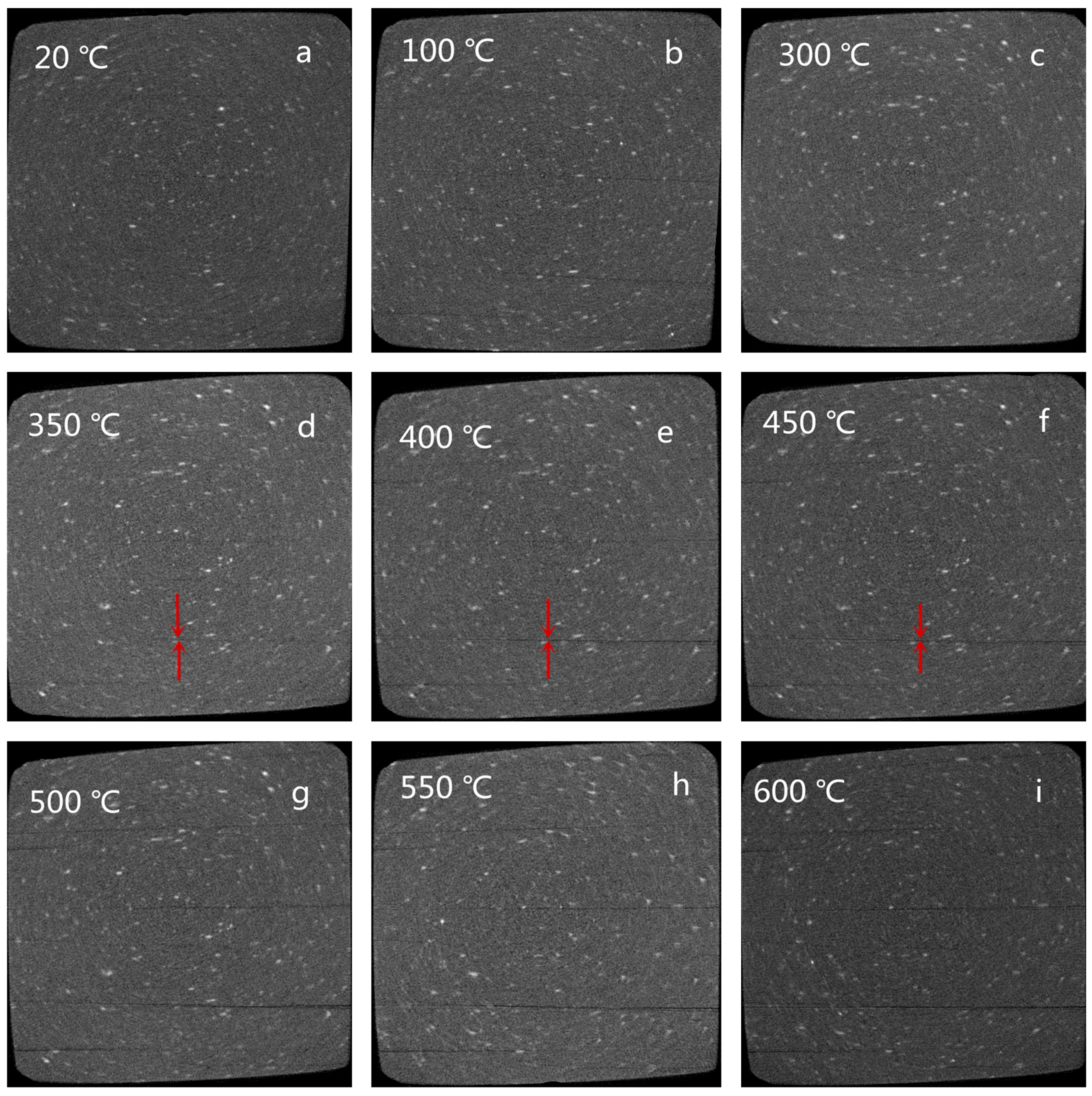
If the rock is a homogeneous material, it will not produce thermal stress [35] when heated in an unconstrained state, and therefore the rock will not have thermal cracking. Because of its sedimentary structure, oil shale shows anisotropy in the directions both parallel and perpendicular to the bedding, and thermal cracking of oil shale at high temperatures also exhibits anisotropy. Figure 9 shows the variation of crack propagation within the oil shale samples both parallel and perpendicular to the bedding planes from 20 °C to 600 °C. The CT data was obtained by micro CT technology and the magnification of the sample was 38. As shown in Figure 10, the crack propagation can be divided into three phases: (1) from 20 °C to 350 °C; (2) from 350 °C, neither cracks along the bedding directions or perpendicular to the bedding directions were found in the samples. A few cracks along the bedding directions were found when the temperature reached 350 °C. At this phase, the main mass loss was due to attached water and bound water [19], which occupied a small proportion within the oil shale. Its liquefaction and vaporization was not enough to produce adequate thermal stress to cause ruptures within the samples. However, at 350 °C, there was a tiny crack where the kerogen began to liquefy and the thermal stress created a tiny crack in the oil sample.
Phase 2 consists of the temperature range of 350 °C to 500 °C. When the specimen was heated to 400 °C, a large number of cracks started to form along the bedding planes. When the temperature was 350 °C, there was only a small crack along the bedding plane, and when the temperature reached 400 °C, the number of large cracks increased. From the TG curve (Figure 5), the kerogen of oil shale began to be pyrolyzed to oil and gas at 400 °C [30], and the oil and gas in the shale expanded synchronously. When the pressure exceeds the tensile strength of oil shale [24], new cracks formed. With the increasing temperature, new cracks continued to form, and the width and length of cracks increased. The kerogen of oil shale continued to be pyrolyzed from 400 °C to 500 °C, increasing the pressure within the sample and expanding the cracks. In this phase, more and more cracks along the bedding directions were found in the shale, and the width of the cracks increased, but the cracks perpendicular to bedding directions were not found in the sample.
Phase 3: From 500 °C to 600 °C, from Figure 9h,i, several new cracks were found in the shale. From the TG curve (Figure 4), the mass loss of the oil shale was tiny, so there was little pyrolysis of oil shale in this phase [31]. Therefore, the pressure of the gas and oil in the shale undergoing pyrolysis was not big enough to create more new cracks. Cracks in the bedding planes perpendicular to bedding directions were still not found in phase 3 temperatures.
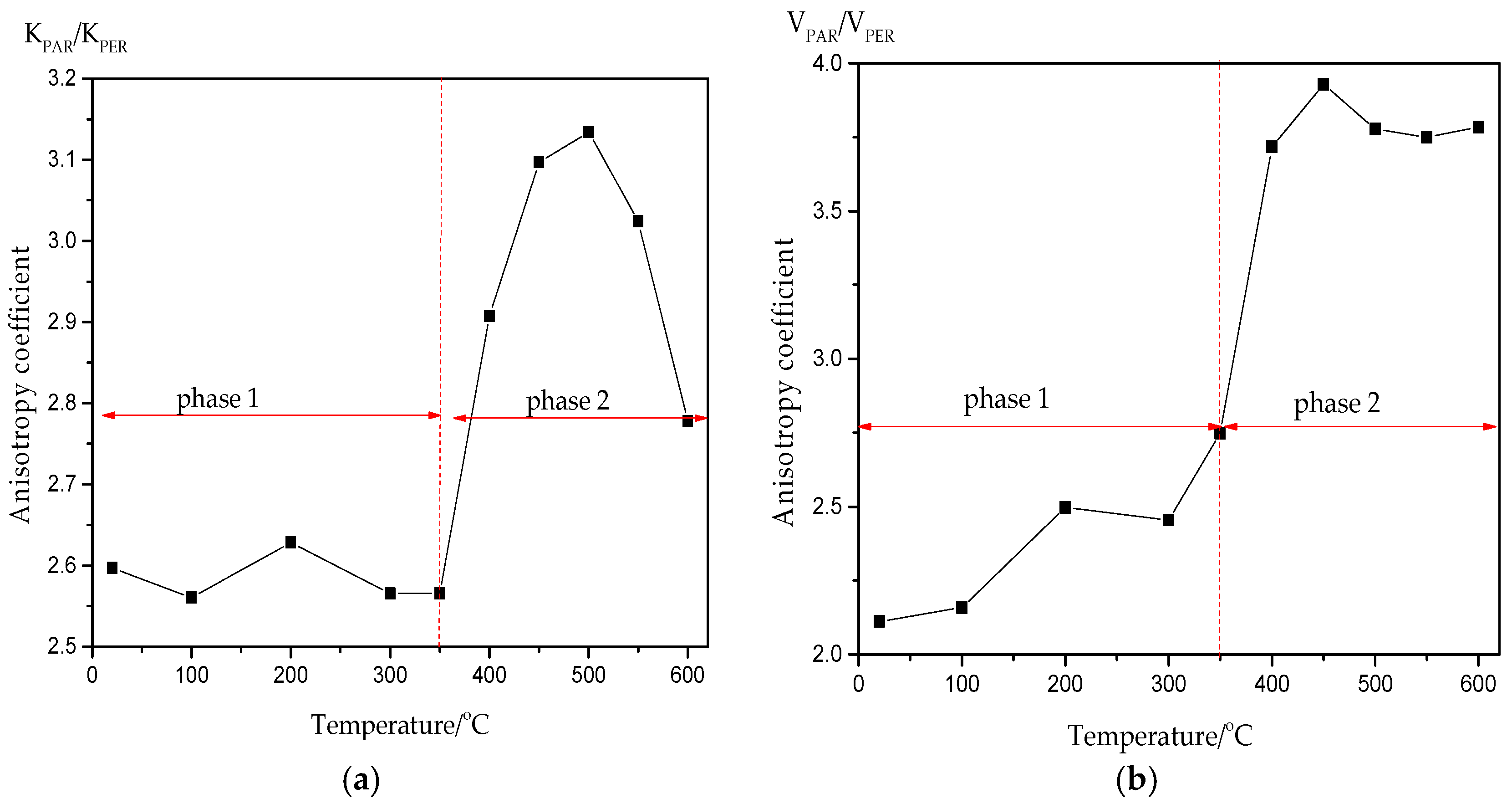
3.4. Variation of Anisotropy Coefficient
The anisotropy coefficient for a parameter is the ratio of the parameter measured for the directions parallel and perpendicular to the bedding. This allows for easy observation of differences along the bedding plane compared to parameters perpendicular to the bedding plane. Figure 10 shows the variation of the anisotropy coefficient of thermal conductivity and P-wave velocity with the temperature. The variation of the anisotropy coefficient with temperature can be divided into two phases: (1) from room temperature to 350 °C, the anisotropy coefficient was basically as a fixed value, as the thermal conductivity and wave velocity decreased linearly with temperature in this phase, as shown in Figure 5; (2) between 350–600 °C, the anisotropy coefficient suddenly increased at 400 °C. A large number of cracks also occurred along the bedding plane at this temperature, leading to a sharp decrease in the thermal conductivity and wave velocity in the direction of the vertical bedding plane. However, the thermal conductivity and wave velocity in the parallel bedding plane still linearly decreased, as shown in Figure 5. These factors led to a sudden increase in the anisotropy coefficient at 400 °C. At 500 °C, the anisotropy coefficient reached its maximum.
4. Discussion
4.1. Reason for the Evolution of Anisotropy of Thermal Conductivity and Wave Velocity
The thermal conductivity and wave velocity of oil shale parallel and perpendicular to the bedding plane greatly vary with an increase in temperature, indicating strong anisotropy. Mineralogy variations and internal material damage can lead to changes in the thermal physical properties of rock [16]. The inhomogeneous expansion of rock and generation of cracks under increasing temperature can also lead to changes of a rock’s thermophysical properties [15]. However, the main reason for the anisotropy of the thermal properties of oil shale is the inhomogeneous expansion of rock and the formation of cracks with the increase in temperature.
Oil shale’s thermal physical property’s anisotropy itself exists because of the bedding structure of the rock, called primary anisotropy. It can be seen from Figure 10 that the initial anisotropy coefficient of heat conduction coefficient is 2.6, and the initial anisotropy coefficient of the wave velocity is 2.1. The experimental results also prove the existence of primary anisotropy of oil shale. In addition to its original anisotropy, many external elements can also lead to changes in rock anisotropy, such as temperature, moisture content, stress status and so on [36]. The anisotropy induced by external factors is what we call induced anisotropy.
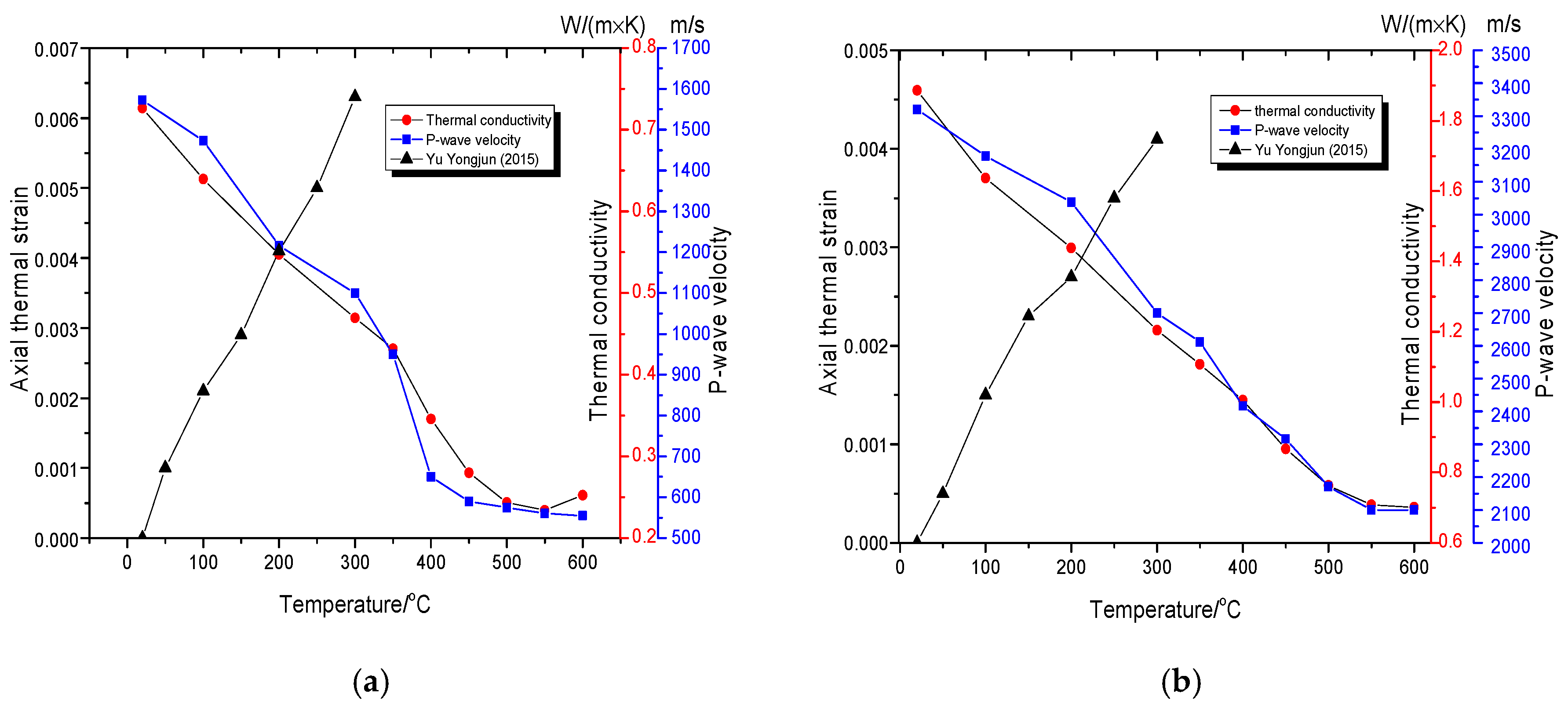
In this paper, we mainly study the influence of temperature on the anisotropy of thermal conductivity and wave velocity of oil shale. It can be seen from Figure 6 that the thermal conductivity and wave velocity decrease linearly with the increase of temperature from room temperature to 350 °C. From the CT results, no obvious cracks appear in this temperature range, and also from Figure 5, the main mass loss of the oil shale material at this stage was attached water and bound water [19]. The proportion of material loss in the pyrolysis process is small. This indicates that the material loss and crack formation are not the reasons for the decreases in wave velocity and thermal conductivity in this temperature range. From room temperature to 300 °C, the mean axial thermal strains both parallel and perpendicular to the bedding directions linearly increase with the increase in the temperature [37]. As shown in Figure 10, the linear decrease of thermal conductivity and P-wave velocity are consistent with the linear increase of thermal strain from room temperature to 300 °C. The main reason for the decrease in both thermal conductivity and P-wave velocity at high temperatures is the expansion of the oil shale within the temperature range from room temperature to 350 °C. At 400 °C, from the CT results, a large number of cracks are generated along the bedding plane, and at the same temperature, the thermal conductivity and wave velocity in the vertical bedding direction decrease significantly. At 400 °C, the thermal conductivity and wave velocity in the parallel bedding direction still decrease linearly, because there is no obvious crack in the perpendicular bedding direction. Moreover, the coefficient of anisotropy of the heat conduction coefficient and wave velocity also increases suddenly at 400 °C. This shows that the crack generation with the increase in temperature is the main reason leading to the anisotropy of the thermal physical parameters of oil shale. Therefore, we can identify 400 °C as the threshold temperature of the evolution of the anisotropy in thermal and physical characteristics of oil shale. With the increase in temperature, the number and width of cracks increase, while the thermal conductivity coefficient and wave velocity in the direction of the perpendicular plane continuously decrease. The thermal conductivity and wave velocity tend be constant from 500 °C to 600 °C because at that temperature range, the mass loss is small and the number and width of cracks no longer increase. The thermal conductivity and velocity parallel to the bedding plane linearly continuously decline from 400 °C to 500 °C, mainly due to the expansion and reduction of rock material. Meanwhile, the thermal conductivity and velocity are constant values from 500 °C to 600 °C, mainly due to lesser amounts of oil shale mass loss.
4.2. Correlation between Thermal Conductivity and P-Wave Velocity
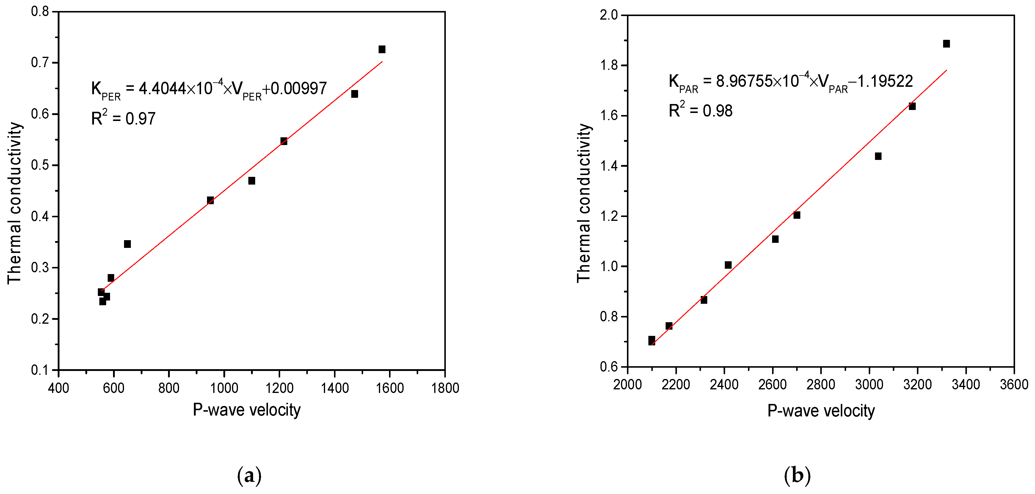
From the variations of thermal conductivity and P-wave velocity both parallel and perpendicular to the bedding planes, the wave velocity changes similarly to that of thermal conductivity, particularly at high temperatures, as shown in Figure 11. Therefore, wave velocity perpendicular to the bedding plane can be used to evaluate the thermal conductivity perpendicular to the bedding plane, as shown in Figure 12a and illustrated by Equation (3). The same formula applies to the wave velocity and thermal conductivity parallel to the bedding planes, as shown in Figure 12b and illustrated by Equation (4):
where KPER is the thermal conductivity in the direction of perpendicular bedding planes, VPER is the wave velocity in the direction of the perpendicular bedding planes, KPAR is the thermal conductivity in the direction of the parallel bedding planes, and VPER is the thermal conductivity in the direction of the parallel bedding planes.
4.3. Experimental Application of the Thermal Recovery of Oil Shale
The experimental results show that the anisotropy of the thermal conductivity and the velocity of the oil shale changes with temperature throughout the heating process. The experimental results also show that the conduction velocity of the temperature in the parallel bedding direction is greater than that in the vertical bedding direction. Therefore, when using a vertical well to extract oil shale, oil shale in the horizontal direction of the heating pipe should first be heated to the pyrolysis temperature of kerogen, while the upper part of the heating pipe is maintained at a relatively low temperature. Through the principles of crack propagation of oil shale at different temperatures, it can be found that there will be many cracks along the bedding direction only when the temperature is greater than 400 °C. The occurrence of these cracks will also provide seepage passages for the pyrolysis of oil and gas from the extraction wells. Therefore, if we control the placement of heating pipes in the oil shale formation, we can control the conduction range of temperature in the oil shale formation, and force the temperature to move along the horizontal direction, so as to reduce the influence of temperature on the overlying strata and floor. In particular, when using vertical wells to extract oil shale, the layout of the horizontal well cannot be arranged according to the layout of the vertical well because of the slow heat conduction velocity in the vertical bedding direction. In order to reasonably calculate the distance between well holes, the research results of this paper can provide a theoretical basis for a rational layout of wellbores. In addition, it was determined that the thermal conductivity of different bedding directions has a linear relationship with the corresponding wave velocity. It is difficult to obtain the heat transfer coefficient in situ, but the velocity measurement can be determined, and the fitting formula of heat conduction and wave velocity can be used as a basis for calculating the thermal conductivity.
5. Conclusions
To study the effect of temperature on the evolution of anisotropy of thermal and physical characteristics of oil shale from room temperature to 600 °C, the thermal diffusion, thermal conductivity, P-wave velocity and crack propagation both perpendicular and parallel to the bedding plane were studied in this paper. The main conclusions are as follows.
- (1)
- Variation in the thermal and physical characteristics perpendicular to the bedding plane can be divided into three phases: (1) from room temperature to 350 °C, the thermal and physical characteristics linearly decreased with the increase in temperature; (2) from 350 °C to 500 °C, thermal and physical characteristics decreased up to 400 °C; (3) thermal and physical characteristics had no obvious change in this phase and values are constant. The variation of the thermal and physical characteristics parallel to the bedding planes can be divided into two phases: (1) from room temperature to 500 °C, the thermal and physical characteristics had a sustained linear decline and the thermal and physical characteristics had no obvious decrease; (2) from 500 °C to 600 °C, the thermal and physical characteristics had no obvious change and finally the value was maintained constant.
- (2)
- Thermal cracks caused by the temperature increase were the main cause for the change of anisotropy ratio and of the thermal and physical characteristics of oil shale. When the temperature reached 400 °C, the number of cracks along the bedding directions increased along with the anisotropy ratio of the thermal and physical characteristics. 400 °C is considered to be the threshold temperature where the change of anisotropy in thermal and physical characteristics occurs.
- (3)
- The variation of thermal conductivity both perpendicular and parallel to the bedding planes with wave velocity can be expressed as Equations (3) and (4). The thermal conductivity has a linear relation with the P-wave velocity.
Acknowledgments
This work was supported by the National Natural Science Foundation of China (51704206, U1261102).
Author Contributions
All authors contributed to the research in the paper. Dong Yang and Guoying Wang. conceived and designed the experiments; Guoying Wang performed the experiments; Jing Zhao and Zhiqin Kang analyzed the data; Guoying Wang wrote the paper.
Conflicts of Interest
The authors declare no conflict of interest.
References
- Burger, J.W.; Crawford, P.M.; Johnson, H.R. Is oil shale America’s answer to peak-oil challenge? Oil Gas J. 2004, 102, 16–24. [Google Scholar]
- Liu, Z.J.; Dong, Q.S.; Ye, S.Q.; Zhu, J.W.; Guo, W.; Li, D.C.; Liu, R.; Zhang, H.L.; Du, J.F. The situation of oil shale resources in China. J. Jilin Univ. (Earth Sci. Ed.) 2006, 36, 869–876, (In Chinese with English abstract). [Google Scholar]
- Vinegar, H. Shell’s in-situ conversion process. In Proceedings of the 26th Oil Shale Symposium, Colorado School of Mines, Golden, CO, USA, 16–18 October 2006; Colorado Energy Research Institute: Golden, CO, USA, 2006. [Google Scholar]
- Kang, Z.Q.; Zhao, Y.S.; Yang, D. Physical principle and numerical analysis of oil shale development using in-situ conversion process technology. Acta Pet. Sin. 2008, 29, 592–595. (In Chinese) [Google Scholar]
- Hillier, J.L.; Fletcher, T.H.; Solum, M.S.; Pugmire, R.J. Characterization of Macromolecular Structure of Pyrolysis Products from a Colorado Green River Oil Shale. Ind. Eng. Chem. Res. 2013, 52, 15522–15532. [Google Scholar] [CrossRef]
- Sun, Y.; Bai, F.; Liu, B.; Liu, Y.; Guo, M.; Guo, W.; Wang, Q.; Lu, X.; Yang, F.; Yang, Y. Characterization of the oil shale products derived via topochemical reaction method. Fuel 2014, 115, 338–346. [Google Scholar] [CrossRef]
- Vernik, L.; Nur, A. Ultrasonic velocity and anisotropy of hydrocarbon source rocks. Geophysics 1992, 57, 727–735. [Google Scholar] [CrossRef]
- Vernik, L.; Landis, C. Elastic anisotropy of source rocks: Implications for hydrocarbon generation and primary migration. AAPG Bull. 1996, 80, 531–544. [Google Scholar]
- Amadei, B. Importance of anisotropy when estimating and measuring in situ, stresses in rock. Int. J. Rock Mech. Min. Sci. Geomech. Abstr. 1996, 33, 293–325. [Google Scholar] [CrossRef]
- Saboorian-Jooybari, H.; Dejam, M.; Chen, Z. Heavy oil polymer flooding from laboratory core floods to pilot tests and field applications: Half-century studies. J. Pet. Sci. Eng. 2016, 142, 85–100. [Google Scholar] [CrossRef]
- Saboorian-Jooybari, H.; Dejam, M.; Chen, Z. Half-century of heavy oil polymer flooding from laboratory core floods to pilot tests and field applications. In Proceedings of the 2015 SPE Canada Heavy Oil Technical Conference (Paper SPE 174402), Calgary, AB, Canada, 9–11 June 2015. [Google Scholar]
- Mashayekhizadeh, V.; Kord, S.; Dejam, M. Eor Potential within Iran. Spec. Top. Rev. Porous Media 2014, 5, 325–354. [Google Scholar] [CrossRef]
- Sun, Q.; Lü, C.; Cao, L.; Li, W.; Geng, J.; Zhang, W. Thermal properties of sandstone after treatment at high temperature. Int. J. Rock Mech. Min. Sci. 2016, 85, 60–66. [Google Scholar] [CrossRef]
- Vosteen, H.D.; Schellschmidt, R. Influence of temperature on thermal conductivity, thermal capacity and thermal diffusivity for different types of rock. Phys. Chem. Earth Parts A B C 2003, 28, 499–509. [Google Scholar] [CrossRef]
- Jha, M.K.; Verma, A.K.; Maheshwar, S.; Chauhan, A. Study of temperature effect on thermal conductivity of Jhiri shale from Upper Vindhyan, India. Bull. Eng. Geol. Environ. 2016, 75, 1657–1668. [Google Scholar] [CrossRef]
- Hajpál, M.; Török, A. Mineralogical and colour changes of quartz sandstones by heat. Environm. Geol. 2004, 46, 311–322. [Google Scholar] [CrossRef]
- Zhao, J.; Yang, D.; Kang, Z.; Feng, Z. A micro-CT study of changes in the internal structure of Daqing and Yan’an oil shales at high temperatures. Oil Shale 2012, 29, 357–367. [Google Scholar] [CrossRef]
- Yang, L.; Yang, D.; Zhao, J.; Liu, Z.; Kang, Z. Changes of oil shale pore structures and permeability at different temperatures. Oil Shale 2016, 33, 101–110. [Google Scholar] [CrossRef]
- Dejam, M.; Hassanzadeh, H.; Chen, Z. Pre-Darcy flow in porous media. Water Resour. Res. 2017, 53, 8187–8210. [Google Scholar] [CrossRef]
- Tiwari, P.; Deo, M.; Lin, C.L.; Miller, J.D. Characterization of oil shale pore structure before and after pyrolysis by using X-ray micro CT. Fuel 2013, 107, 547–554. [Google Scholar] [CrossRef]
- Bai, F.; Sun, Y.; Liu, Y.; Guo, M. Evaluation of the porous structure of Huadian oil shale during pyrolysis using multiple approaches. Fuel 2017, 187, 1–8. [Google Scholar] [CrossRef]
- Junwei, Y.; Xiumin, J.; Xiangxin, H.; Jianguo, L. A TG-FTIR investigation to the catalytic effect of mineral matrix in oil;shale on the pyrolysis and combustion of kerogen. Fuel 2013, 104, 307–317. [Google Scholar]
- Kang, Z.; Yang, D.; Zhao, Y.; Hu, Y.Q. Thermal cracking and corresponding permeability of Fushun oil shale. Oil Shale 2011, 28, 273–283. [Google Scholar] [CrossRef]
- Meng, Q.R.; Kang, Z.Q.; Zhao, Y.S.; Dong, Y. Experiment of thermal cracking and crack initiation mechanism of oil shale. Zhongguo Shiyou Daxue Xuebao 2010, 34, 89–92. [Google Scholar]
- Diansen, Y.; Chanchole, S.; Valli, P.; Chen, L. Study of the Anisotropic Properties of Argillite under Moisture and Mechanical Loads. Rock Mech. Rock Eng. 2013, 46, 247–257. [Google Scholar]
- Masri, M.; Sibai, M.; Shao, J.F.; Mainguy, M. Experimental investigation of the effect of temperature on the mechanical behavior of Tournemire shale. Int. J. Rock Mech. Min. Sci. 2014, 70, 185–191. [Google Scholar] [CrossRef]
- Kim, H.; Cho, J.W.; Song, I.; Min, K.B. Anisotropy of elastic moduli, P-wave velocities, and thermal conductivities of Asan Gneiss, Boryeong Shale, and Yeoncheon Schist in Korea. Eng. Geol. 2012, 147–148, 68–77. [Google Scholar] [CrossRef]
- Cho, J.W.; Kim, H.; Jeon, S.; Min, K.B. Deformation and strength anisotropy of Asan gneiss, Boryeong shale, and Yeoncheon schist. Int. J. Rock Mech. Min. Sci. 2012, 50, 158–169. [Google Scholar] [CrossRef]
- Özkahraman, H.T.; Selver, R.; Işık, E.C. Determination of the thermal conductivity of rock from P-wave velocity. Int. J. Rock Mech. Min. Sci. 2004, 41, 703–708. [Google Scholar] [CrossRef]
- Saif, T.; Lin, Q.; Singh, K.; Bijeljic, B.; Blunt, M.J. Dynamic imaging of oil shale pyrolysis using synchrotron X-ray microtomography. Geophys. Res. Lett. 2016, 43, 6799–6807. [Google Scholar] [CrossRef]
- Saif, T.; Lin, Q.; Bijeljic, B.; Blunt, M.J. Microstructural imaging and characterization of oil shale before and after pyrolysis. Fuel 2017, 197, 562–574. [Google Scholar] [CrossRef]
- Parker, W.J.; Jenkins, R.J.; Butler, C.P.; Abbott, G.L. Flash Method of Determining Thermal Diffusivity, Heat Capacity, and Thermal Conductivity. J. Appl. Phys. 1961, 32, 1679–1684. [Google Scholar] [CrossRef]
- Qian, J.L.; Yin, L. Oil Shale—The Supply Resource for Petroleum; Petrochemical Press: Beijing, China, 2008; pp. 50–51. (In Chinese) [Google Scholar]
- Zhao, Y.X.; Yang, S.Z.; Zhang, W.R.; Ma, L. An experimental study of rock thermal conductivity under different temperature and pressure. Prog. Geophys. 1995, 10, 104–113. [Google Scholar]
- Kingery, W.D. Factors Affecting Thermal Stress Resistance of Ceramic Materials. J. Am. Ceram. Soc. 1955, 38, 3–15. [Google Scholar] [CrossRef]
- Nagaraju, P.; Roy, S. Effect of water saturation on rock thermal conductivity measurements. Tectonophysics 2014, 626, 137–143. [Google Scholar] [CrossRef]
- Yu, Y. Reasearch on Fracture and Damage Behaviour of Oil Shale under Thermal-Mechanical Coupling Field; Taiyuan University of Technology: Taiyuan, China, 2015. (In Chinese) [Google Scholar]
Figure 1.
Schematic diagram of in-situ mining of oil shale: (a) Shell’s in-situ conversion process (ICP) technology; and (b) In-situ steam injection technology of TYUT (Taiyuan University of Technology).
Figure 1.
Schematic diagram of in-situ mining of oil shale: (a) Shell’s in-situ conversion process (ICP) technology; and (b) In-situ steam injection technology of TYUT (Taiyuan University of Technology).
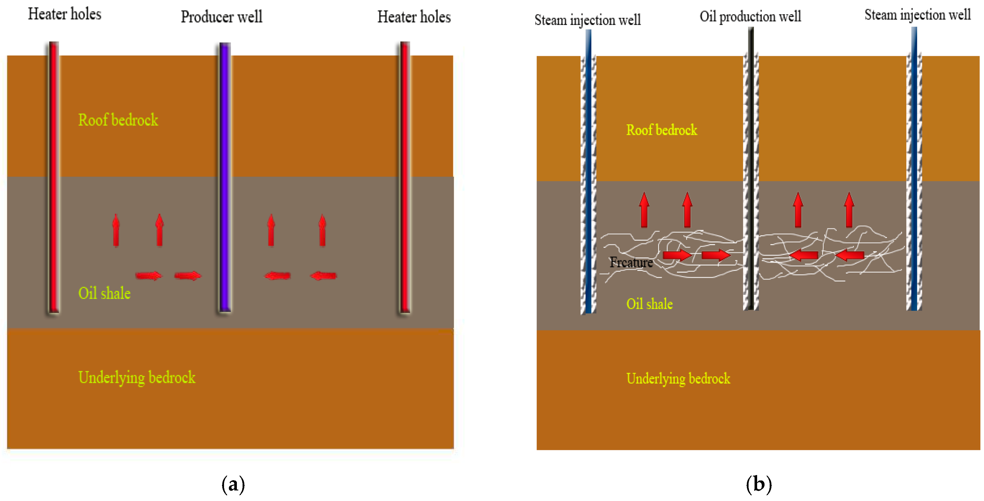
Figure 2.
Schematic diagram of heat conduction and acoustic conduction, (a) parallel to bedding plane; and (b) perpendicular to bedding plane.
Figure 2.
Schematic diagram of heat conduction and acoustic conduction, (a) parallel to bedding plane; and (b) perpendicular to bedding plane.

Figure 3.
Main experimental instruments: (a) Netzsch LFA 457 laser thermal conductivity analyzer; (b) STA 449 F3 synchronous thermal analyzer; (c) micro CT experimental system; and (d) SYC-2 acoustic wave rock parameter test instrument.
Figure 3.
Main experimental instruments: (a) Netzsch LFA 457 laser thermal conductivity analyzer; (b) STA 449 F3 synchronous thermal analyzer; (c) micro CT experimental system; and (d) SYC-2 acoustic wave rock parameter test instrument.

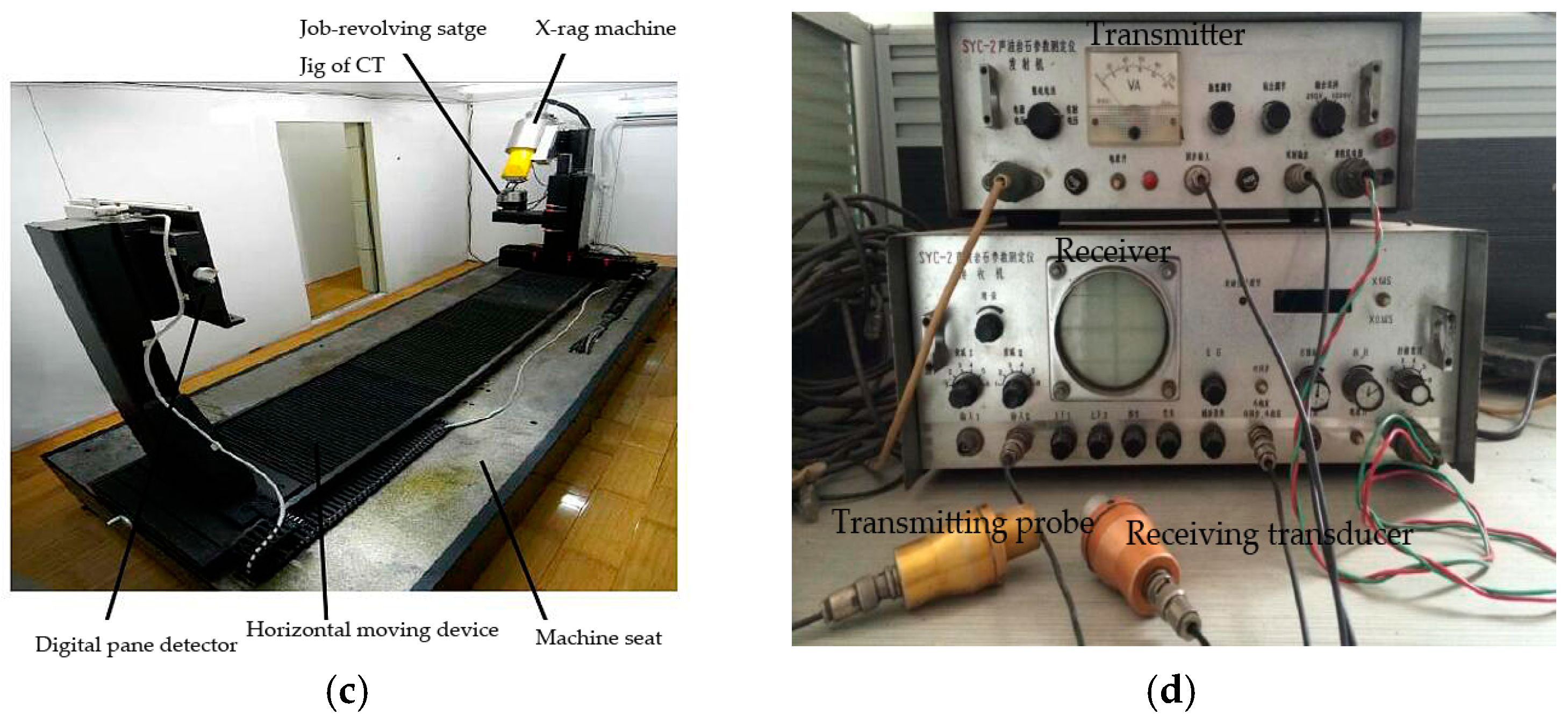
Figure 4.
Schematic diagram of CT (Computed Tomography) heating furnace.

Figure 5.
Thermal analysis of oil shale (DSC: for differential scanning calorimetry; TG: thermogravimetric).
Figure 5.
Thermal analysis of oil shale (DSC: for differential scanning calorimetry; TG: thermogravimetric).

Figure 6.
Variation of thermal conductivity and thermal diffusion with temperature (a) perpendicular to bedding planes; and (b) parallel to bedding planes.
Figure 6.
Variation of thermal conductivity and thermal diffusion with temperature (a) perpendicular to bedding planes; and (b) parallel to bedding planes.
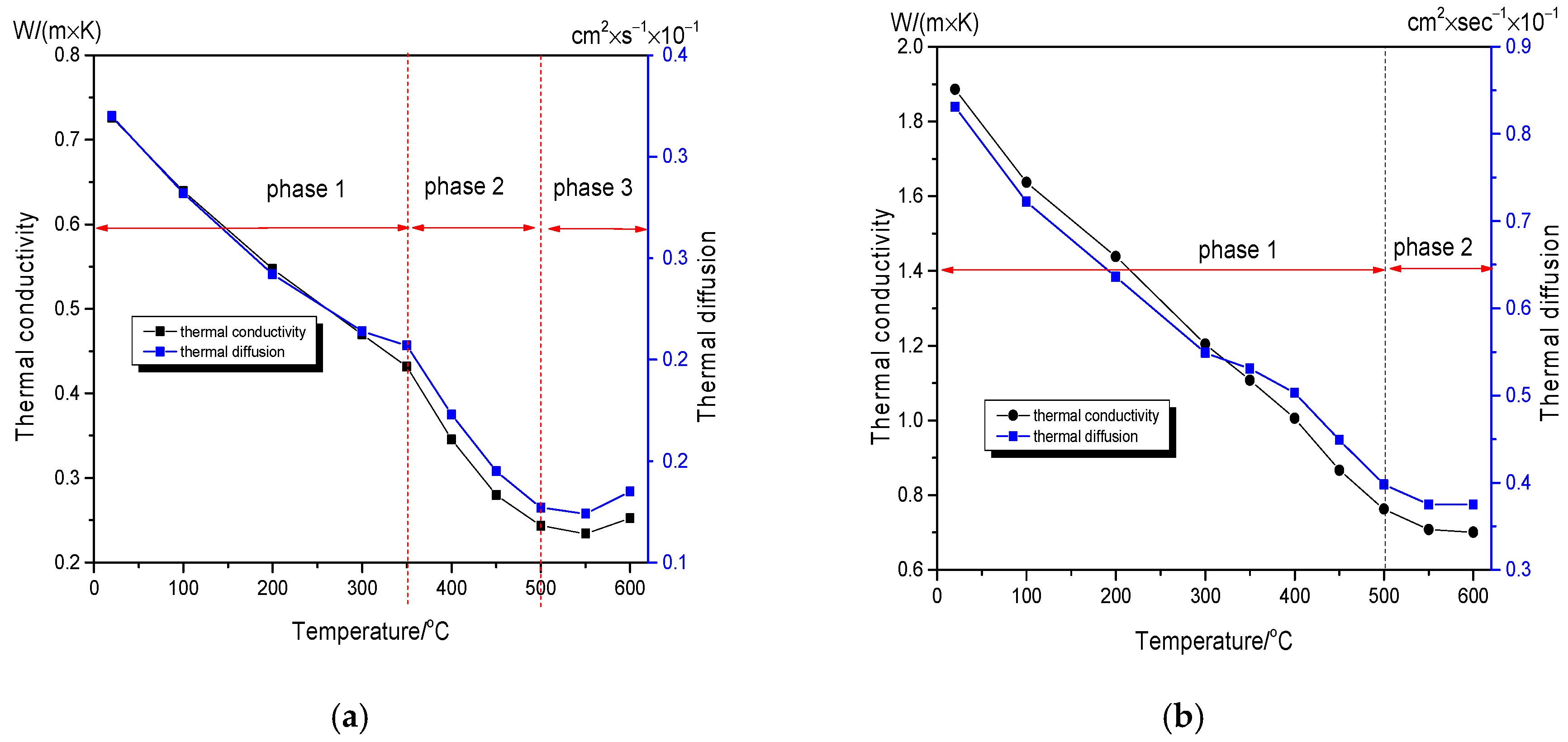
Figure 7.
Variations of P-wave velocity with temperature (a) perpendicular to bedding planes; and (b) parallel to bedding planes.
Figure 7.
Variations of P-wave velocity with temperature (a) perpendicular to bedding planes; and (b) parallel to bedding planes.
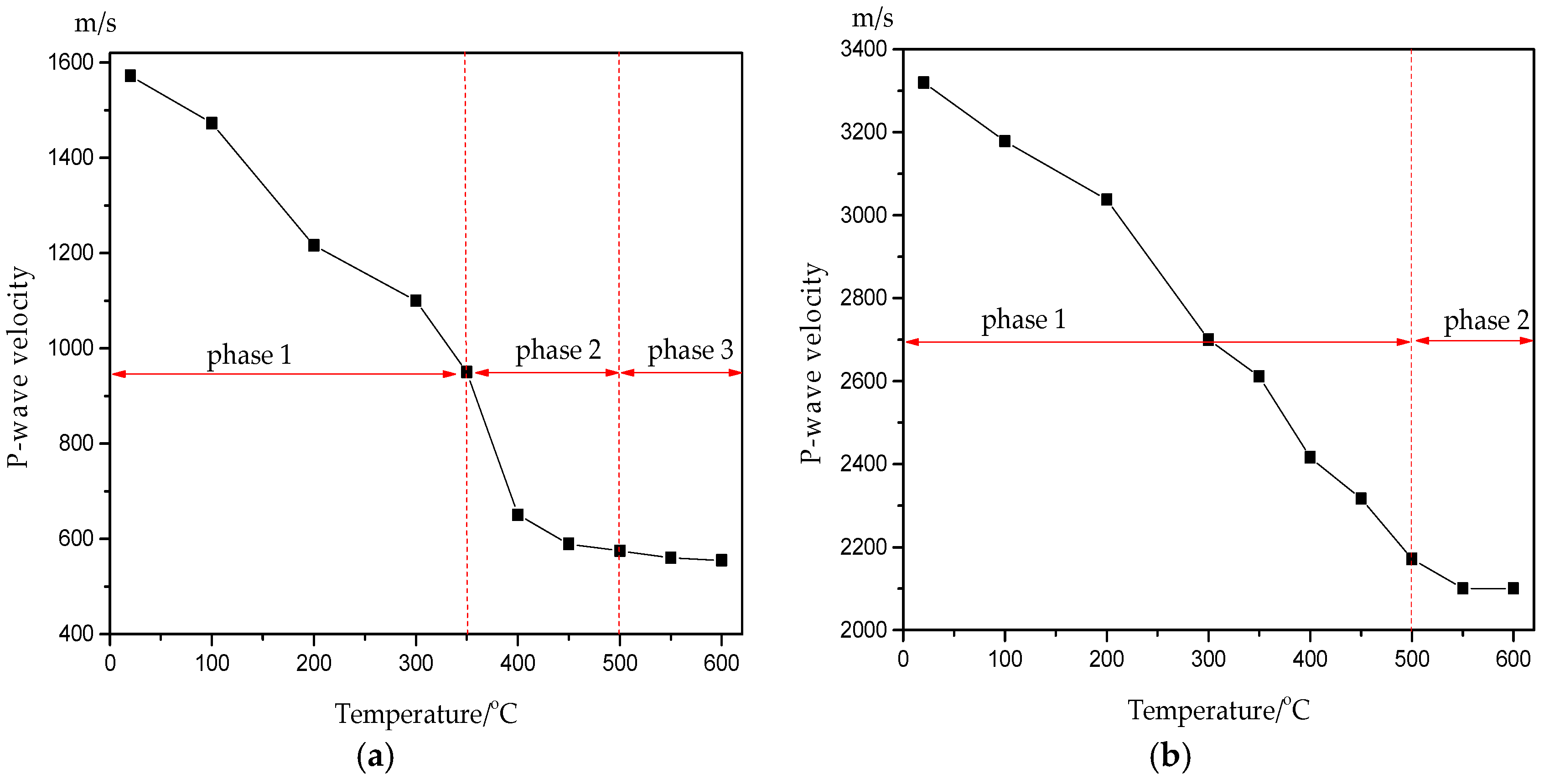
Figure 8.
Variation of damage coefficient with temperature at high temperature.
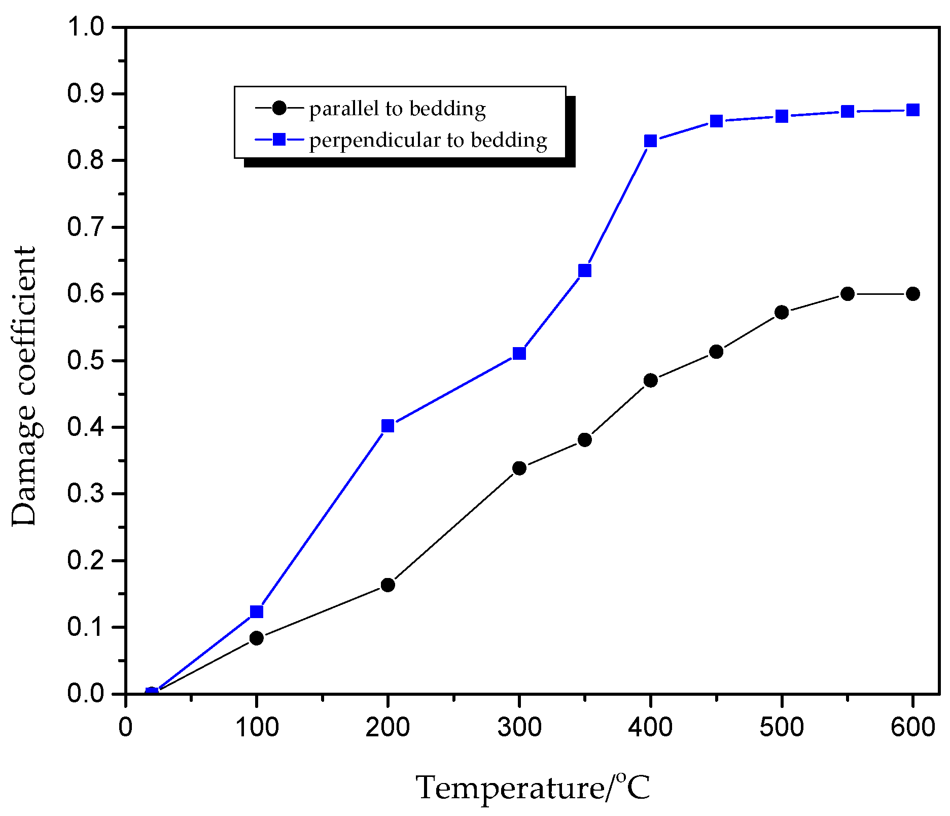
Figure 9.
Thermal crack propagation scanning by CT at different temperatures at 38× magnification.

Figure 10.
Variation of anisotropy coefficient with temperature: (a) anisotropy coefficient of thermal conductivity; and (b) anisotropy coefficient of P-wave velocity.
Figure 10.
Variation of anisotropy coefficient with temperature: (a) anisotropy coefficient of thermal conductivity; and (b) anisotropy coefficient of P-wave velocity.

Figure 11.
Variation of thermal conductivity, P-wave velocity and thermal expansion with temperature (a) perpendicular to bedding planes; and (b) parallel to bedding planes.
Figure 11.
Variation of thermal conductivity, P-wave velocity and thermal expansion with temperature (a) perpendicular to bedding planes; and (b) parallel to bedding planes.

Figure 12.
Correlation between thermal conductivity with P-wave velocity (a) perpendicular to bedding planes; and (b) parallel to bedding planes.
Figure 12.
Correlation between thermal conductivity with P-wave velocity (a) perpendicular to bedding planes; and (b) parallel to bedding planes.


Table 1.
Shape and sizes of samples for different kinds of experiment (DSC: for differential scanning calorimetry; TG: thermogravimetric).
Table 1.
Shape and sizes of samples for different kinds of experiment (DSC: for differential scanning calorimetry; TG: thermogravimetric).
| Experiment | Thermal Diffusion | DSC–TG | Wave Velocity | CT Scanning |
|---|---|---|---|---|
| Sample shape | Block | Cylinder | Cylinder | Block |
| Size | 10 × 10 × 2 mm | 5 × 1 mm | 10 × 25 mm | 7 × 7 × 7 mm |
| Sample bedding plane | Perpendicular and parallel to bedding plane | - | Perpendicular and parallel to bedding plane | Perpendicular and parallel to bedding plane |
Table 2.
Calculation coefficients for Equation (1) (DPER: Thermal diffusion of perpendicular to bedding, DPAR: Thermal diffusion of parallel to bedding, KPER: Thermal conductivity of perpendicular to bedding, KPAR: Thermal conductivity of parallel to bedding).
Table 2.
Calculation coefficients for Equation (1) (DPER: Thermal diffusion of perpendicular to bedding, DPAR: Thermal diffusion of parallel to bedding, KPER: Thermal conductivity of perpendicular to bedding, KPAR: Thermal conductivity of parallel to bedding).
| Calculation Coefficients | 20 °C | 100 °C | 200 °C | 300 °C | 350 °C | 400 °C | 450 °C | 500 °C | 550 °C | 600 °C | |
|---|---|---|---|---|---|---|---|---|---|---|---|
| Thermal diffusion | DPER | 0.32 | 0.282 | 0.242 | 0.214 | 0.207 | 0.173 | 0.145 | 0.127 | 0.124 | 0.135 |
| DPAR | 0.831 | 0.722 | 0.636 | 0.549 | 0.531 | 0.503 | 0.449 | 0.398 | 0.375 | 0.375 | |
| Density (g/cm3) | 2.176 | 2.174 | 2.168 | 2.103 | 2.01 | 1.917 | 1.852 | 1.838 | 1.811 | 1.792 | |
| Thermal conductivity | KPER | 0.726 | 0.639 | 0.547 | 0.469 | 0.431 | 0.356 | 0.279 | 0.243 | 0.234 | 0.252 |
| KPAR | 1.886 | 1.637 | 1.438 | 1.204 | 1.108 | 1.006 | 0.866 | 0.763 | 0.708 | 0.701 | |
© 2018 by the authors. Licensee MDPI, Basel, Switzerland. This article is an open access article distributed under the terms and conditions of the Creative Commons Attribution (CC BY) license (http://creativecommons.org/licenses/by/4.0/).
Share and Cite
MDPI and ACS Style
Wang, G.; Yang, D.; Kang, Z.; Zhao, J. Anisotropy in Thermal Recovery of Oil Shale—Part 1: Thermal Conductivity, Wave Velocity and Crack Propagation. Energies 2018, 11, 77. https://doi.org/10.3390/en11010077
AMA Style
Wang G, Yang D, Kang Z, Zhao J. Anisotropy in Thermal Recovery of Oil Shale—Part 1: Thermal Conductivity, Wave Velocity and Crack Propagation. Energies. 2018; 11(1):77. https://doi.org/10.3390/en11010077
Chicago/Turabian StyleWang, Guoying, Dong Yang, Zhiqin Kang, and Jing Zhao. 2018. "Anisotropy in Thermal Recovery of Oil Shale—Part 1: Thermal Conductivity, Wave Velocity and Crack Propagation" Energies 11, no. 1: 77. https://doi.org/10.3390/en11010077
Note that from the first issue of 2016, this journal uses article numbers instead of page numbers. See further details here.