Hourly Solar Radiation Forecasting Using a Volterra-Least Squares Support Vector Machine Model Combined with Signal Decomposition


Key Laboratory of Advanced Process Control for Light Industry (Ministry of Education), Jiangnan University, Wuxi 214122, China
*
Author to whom correspondence should be addressed.
Energies 2018, 11(1), 68; https://doi.org/10.3390/en11010068
Submission received: 27 November 2017
/
Revised: 17 December 2017
/
Accepted: 18 December 2017
/
Published: 1 January 2018
Abstract
:Accurate solar forecasting facilitates the integration of solar generation into the grid by reducing the integration and operational costs associated with solar intermittencies. A novel solar radiation forecasting method was proposed in this paper, which uses two kinds of adaptive single decomposition algorithm, namely, empirical mode decomposition (EMD) and local mean decomposition (LMD), to decompose the strong non-stationary solar radiation sequence into a set of simpler components. The least squares support vector machine (LSSVM) and the Volterra model were employed to build forecasting sub-models for high-frequency components and low-frequency components, respectively, and the sub-forecasting results of each component were superimposed to obtain the final forecast results. The historical solar radiation data collected on Golden (CO, USA), in 2014 were used to evaluate the accuracy of the proposed model and its comparison with that of the ARIMA, the persistent model. The comparison demonstrated that the superior performance of the proposed hybrid method.
1. Introduction
Solar radiation is the most important factor affecting photovoltaic power generation [1]. Accurate solar forecasting facilitates the integration of solar generation into the grid by reducing the integration and operational costs associated with solar intermittencies [2]. Nowadays, physically- based forecasting is mainly conducted using numerical weather prediction methods such as the well-known numerical weather prediction (NWP), which provides information up to several days ahead; however, it has obvious biases and random errors [3]. It is therefore very important to develop effective solar radiation forecasting methods, especially ones that can use less measurements. Solar radiation sequences can be treated as a time series produced by random processes; therefore, mathematical models can be used to fit the underlying processes and forecast the future values [4,5]. Many modeling methods have been used to describe solar radiation sequences, including regression methods such as linear regression [4], autoregressive model (AR) [6], autoregressive moving average (ARMA) [7], multi-dimensional linear prediction filters [8], least absolute shrinkage and selection operator (LASSO) [9], and nonlinear model approximators such as artificial neural network (ANN) [10], adaptive neuro-fuzzy inference system [11], hidden Markov model [12], fuzzy logic [13] and Angstrom–Prescott equations [14]. Traditionally, these techniques were used independently by researchers to build forecasting models for solar radiation. However, solar radiation is a strong random process, which makes a single modeling algorithm unable to guarantee the accuracy and robustness of the forecasting model. Therefore, hybrid models were used to maximize the advantages of different models. Theoretical and empirical results suggest that hybrid methods can effectively improve the prediction performance [15].
Hybrid methods are categorized into algorithm hybrids, data hybrids, and joint hybrids of algorithms and data. Algorithm hybrids use preprocessing algorithms to decompose or classify the original solar radiation sequence into a series of stationary components that are easier to model and predict, and then the forecasting models for each component were built according to the characteristic of the components [15,16,17]. Because the solar radiation is influenced by climatic and environmental parameters, the robustness of forecast models based on the historical data of solar radiation may not be guaranteed. To address this limitation, researchers proposed the data hybrid method, which integrates solar radiation data and meteorological parameters to develop a forecast model of solar radiation [18,19]. Aiming to capture the distribution characteristics of solar radiation and meteorological parameters more effectively, the joint hybrid of data and algorithms method is proposed. Then, the forecast model for data distribution using different modeling algorithms is established [20,21].
However, the modeling methods for solar radiation using data hybrids or joint hybrids of data and algorithms require available meteorological and environmental parameters. These parameters are usually difficult to obtain in practical application because of the expensive price of measuring equipment and the installation limits. Hence, a novel hybrid method, which only depends on the historical data of the solar radiation, was proposed in this study to realize the accurate forecast of solar radiation without high cost. The proposed modeling method employs two kinds of adaptive signal decomposition methods, namely, EMD and LMD, to adaptively decompose the strong non-stationary solar radiation sequence into a set of simpler components. Following that, the LSSVM and the Volterra model were used to build sub-models for different components. The final forecasting results were obtained by integrating all of sub-models. The comparison results demonstrated that the superior performance of the proposed hybrid method.
This work is organized as follows: the data used in the study are described in Section 2. The method used in this study is explained in Section 3. Evaluation metrics for the model performance comparison are listed in Section 4. Simulation experiments with different algorithms and comparison results are presented in Section 5. Finally, conclusions are made in Section 6.
2. Data Description
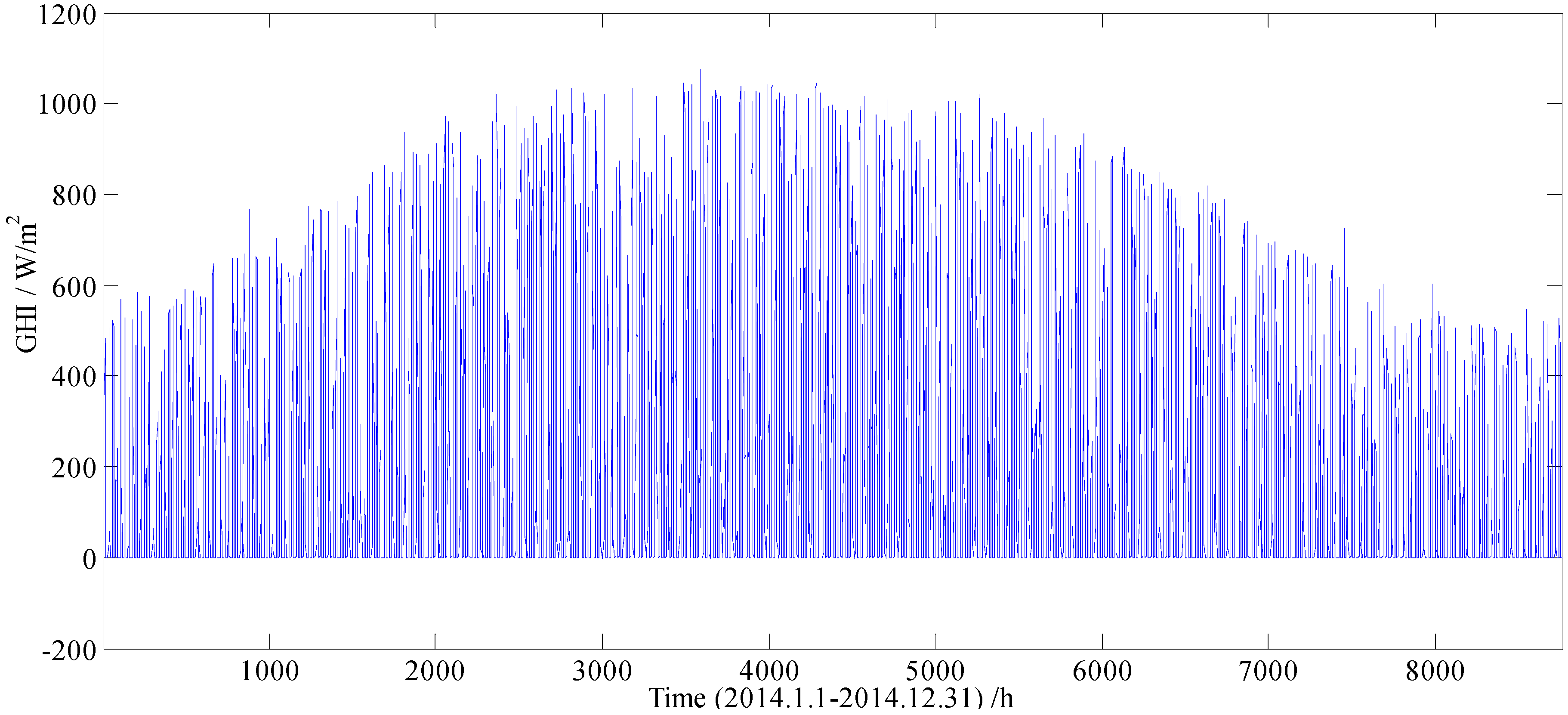
The time series of hourly Global Horizontal Irradiance (GHI, which means hourly average value), collected on Golden, CO, USA (39.7° N, 105° W, 1829 m AMSL) in 2014, were used in this study. These GHI data were acquired by using a high-precision CM22 pyranometer instrument on a plane surface, and can be downloaded from the website of National Renewable Energy Laboratory (NREL, URL link: http://www.nrel.gov/midc/srrl_bms/).
Colorado is a mountain state with a complex climate. Table 1 presents the information about temperatures and relative humidity (RH) of the observation site in 2014. It can be seen that the observed environmental volatility is strong. The strong environmental volatility will result in strong nonstationary of solar radiation sequence, and ultimately lead to difficulty in establishing an accurate forecasting model. Therefore, the solar radiation sequence of Colorado in 2014 was used to verify the performance of the proposed method.
The series of hourly Global Horizontal Irradiance (GHI) values used in this study is shown in Figure 1, which contains a total of 8760 sampling data, and each sampling data represents an average value of hourly GHI, and there are 24 sample points per day. From Figure 1, it can be found that the seasonal factor has a great impact on the GHI. In order to weaken the influence of seasonal factor on the forecasting performance of the model, a total of 8760 sampling data were divided into 4 datasets (i.e., 1 January to 31 March, 1 April to 30 June, 1 July to 30 September, 1 October to 31 December), according to their sampling date.
The forecasting model was established for each dataset. Considering the adaptive signal decomposition algorithms used in this study are based on the prior condition of the time-continuity of the original signal, in order to satisfy this condition, the first 70% sampling data of each dataset were used as training set, and the last 30% sampling data were used as testing set. When the number of samples is sufficient, this sample partitioning method can cover all possible weather situations.
3. Methodology
3.1. Signal Decomposition
The original solar radiation series has strong nonlinear and nonstationary characteristics. Existing modeling methods have limited ability to describe this kind of signal. Hence, the adaptive signal decomposition algorithms were used to decompose original solar radiation into a small number of simpler components (sub-sequences) to improve prediction accuracy. EMD and LMD have been extensively shown as good and popular adaptive methods for processing nonlinear and nonstationary signals. They were widely used in many applications, such as solar radiation forecasting [16], energy load forecasting [22], climate forecasting [23], and time-frequency estimation for electroencephalogram [24]. Because the EMD and LMD have different decomposition mechanisms, the sub-sequences obtained by these two methods also have some differences, which are exactly the description of the original signal from different perspectives. Considering the complexity of the original solar radiation sequence, the EMD and LMD methods were used for analysis and comparison simultaneously in this study to realize the multi-angle and comprehensive description for original solar radiation sequence.
3.1.1. Empirical Mode Decomposition
The basic idea of EMD is to decompose a complicated signal into a finite and a small number of oscillatory modes based on a local characteristic time scale. Each oscillatory mode is expressed by an intrinsic mode function (IMF), which has to satisfy the following two conditions: (1) In the whole dataset, the number of extrema and the number of zero-crossings must either be equal or differ at most by one; (2) At any point, the mean between the upper and lower envelopes must be zero. Let be a given solar radiation sequence, the computational steps of the EMD are described as follows:
Step 1. Identify all the local extrema of I(t) and connect all the local maxima and minima using a cubic spline to generate an upper envelope u(t) and a lower envelope v(t).
Step 2. Calculate the mean envelop m(t) by averaging the upper envelope u(t) and the lower envelope v(t), and then subtract it from I(t) to obtain a detailed component d(t) = I(t) − m(t).
Step 3. Check whether d(t) is an IMF. If d(t) is an IMF, then set c(t) = c(t) and meanwhile replace I(t) with the residual r(t) = I(t) − d(t). Otherwise, replace I(t) with d(t)and repeat Steps 1–2, until the following termination criterion is satisfied:
where j denotes the number of iterative calculations. The threshold value was set to 0.25 in this study.
Step 4. Repeat Steps 1–3, until all the IMFs and residual are obtained. Finally, the original time series I(t) can be decomposed as follows:
where ci(t) and r(t) represent different IMFs and final residual, respectively. Here, the number of IMFs is adaptively determined by the algorithm. For complete procedures, please refer to the references [25,26].
3.1.2. Local Mean Decomposition
LMD was originally developed for decomposing the modulated signals into a small set of product functions (PFs), each of which is the product of an amplitude envelope signal and a frequency modulated signal. LMD scheme involves progressively separating a frequency modulated signal from an amplitude envelope signal in essence. For a given solar radiation sequence I(t), the procedure of LMD can be simply described as follows:
Step 1. Identify the local extrema ni from I(t), and calculate the mean value mi and magnitude ai of the two successive extrema ni and ni+1 using the following description:
Step 2. Smooth local means and local magnitudes using moving averaging respectively, to form a smoothly varying continuous local mean function m(t) and the envelope function a(t), and calculate the assessment function s(t) as follows:
Step 3. Replace I(t) with s(t) and repeat Steps 1–2, until the envelope function a(t) equals 1, and finally the product function (PF) is obtained:
where j denotes the number of iterative calculation, aj(t) is the envelope function obtained in the j-th iterative process, and sn(t) is the final assessment function.
Step 4. Replace the original signal I(t) with the residual r(t) = I(t) − PF(t), repeat Steps 1–3, until the residual r(t) is a constant or monotonic. Finally, the original time series I(t) can be decomposed as follows:
where PFi(t) and r(t) represent different PFs and final residual, respectively. Like the EMD algorithm, the number of PFs is also adaptively determined by the algorithm. Interested readers may refer to [27] for details.
3.2. False Nearest Neighbor (FNN) Algorithm
After decomposition, each component obtained by the EMD or the LMD can be treated as a time series produced by the dynamical system. According to state space equation, for a given time series {x(t), t = 1, .., k, …, j, …N}, produced by the dynamical system, their relationship can be described as the following equation:
where F(·) is a nonlinear function reflecting the relationship between ‘input’ vectors x(t−1) and ‘output’ values , and m is an embedding dimension reflecting time-delay characters of the dynamical system.
The objective of time series prediction is to obtain the function F(·) based on the given time series {x(t), t = 1, .., k, …, j, …N}, using various modeling methods. When the function F(·) (also called forecasting model) is established, the next value can be predicted using the m-dimension vector {x(t), x(t − 1), …, x(t − m + 1)}. However, due to the lack of prior knowledge of the dynamic system, the proper embedding dimension of the dynamic system is unknown. Therefore, determining the embedding dimension (also called input dimension of the forecasting model) must be done before developing the forecasting model. The false nearest neighbor algorithm (FNN) [28] was adopted to confirm the optimal embedding dimension in this study. The FNN algorithm was summarized as follows:
Step 1. For a given small embedding dimension m, identify the closest point (in the Euclidean sense) to a given point in the time-delay coordinates. That is, for a given time-delay point Xm(k) = [x(k), x(k − 1), …, x(k − m + 1)], find the point Xm(j) in the data set such that the following distance d is minimized:
Xm(j) is known as the nearest neighbor to Xm(k).
Step 2. Determine if the following expression is true or false:
where R is threshold value, and set as 1/15 in this study. If expression (9) is true, then the neighbors are true nearest neighbors. If the expression is false, then the neighbors are false nearest neighbors.
Step 3. Continue the algorithm for all points k in the data set. Calculate the percentage of points in the data set which have false nearest neighbors.
Step 4. Continue the algorithm for increasing embedding dimension m until the percentage of false nearest neighbors drops to acceptably small number. In this study, if for a certain m, the percentage of false nearest neighbors is less than 5%, it is accepted as the embedding dimension for the data set.
3.3. Prediction Model
After decomposition, selecting an effective modeling method to build the forecasting model for each component is particularly important. The Volterra model and the LSSVM are two powerful and popular modeling tools in nonlinear and nonstationary time series analysis. By integrating linear and nonlinear factors of the nonlinear time series, the Volterra model can automatically track the chaotic trajectory and yield accurate forecasting results for nonlinear time series [29]. However, as a polynomial regression model, the Volterra model is difficult to obtain satisfied forecasting results for strong nonlinear time series due to the influence of finite model orders. The support vector machine (SVM) is a machine learning method based on structural risk minimization coupled with kernel mapping, which can achieve the best generalization ability of model by balancing the model complexity and learning ability [30]. As an improved version of the SVM, the LSSVM uses equality constraints to replace inequality constraints of the SVM; therefore, it has a faster computing speed while maintaining the generalization ability [31]. The LSSVM can obtain better results than that of the Volterra model for strong nonlinear time series forecasting by using a kernel function. Considering each component obtained by the EMD and the LMD has different nonlinear characteristics, high-frequency components have stronger nonlinearity than low-frequency components. LSSVM was thus used to model the high-frequency components while the Volterra was used to model the low-frequency components. Finally, the best forecasting model was achieved by integrating different sub-models.
3.3.1. Least Squares Support Vector Machine
LSSVM is an effective regression method based on the SVM, the quadratic optimization of the LSSVM is solving linear equations by constructing a loss function, which reduces the computational complexity, improves computation speed, and positively influences regression modeling. It has been widely used in time-series prediction [32].
Given X(t) = [x(t), x(t − 1), …, x(t − m + 1)] and Y(t) = x(t + 1) are set as the input and output of a nonlinear discrete dynamic system, respectively, the initial space has the following form:
where ψ(X(t)) is the nonlinear mapping function, which maps X(t) to the high dimensional feature space. According to the structural risk minimization principle, the optimization problem can be expressed as:
where γ is the regularization parameter, and is a given training set, ei(t) is the error variable. When the dimension tends to be infinite, the Lagrange duality problem can be set up to solve the above problem. The solution to this problem is presented by Suykens and Vandewalle [33] as:
where K(X(t), Xi(t)) is the kernel function. In this paper, the radial basis function (RBF) was selected as the kernel function:
where σ2 is the kernel function parameter. The regularization parameter γ and the kernel function parameter σ2 control the model complexity and affect the generalization capability of the LSSVM. In this study, the grid-search algorithm coupled with the 10-fold cross validation was utilized to optimize these two parameters. Relevant reference [34] may help the reader to get a clear idea on how the LSSVM works.
3.3.2. Volterra Model
The Volterra model is a general mathematical model for a nonlinear system that produces a single output from a serial input. The Volterra models can fit any dynamic systems, without necessity to assume the model structure [35,36]. Given and are the input and output of a nonlinear dynamic system, respectively. The discrete form of the Volterra model is written as:
where hp(m1, m2, …, mp) is the p order Volterra kernel, which act as the weighting coefficients on the past input to the system. This infinite series expansion is difficult to be realized in practical applications; thus, the form of finite truncated and finite times must be used. The most commonly used form is the following two-order truncation sum:
the coefficients of the Volterra model expressed in Equation (15) can be solved using the orthogonal decomposition, stepwise multiple regression, and the iterative descent gradient method. In this paper, the least square algorithm was adopted. Complete details of the Volterra may refer to consistent reference [37].
4. Model Evaluation
In this paper, four statistical parameters, including Root mean square error (RMSE), mean absolute error (MAE), correlation coefficient (R), and forecast skill were used in model evaluation.
4.1. Root Mean Square Error
Root mean square error can be obtained using the following equation:
where and x(t) are the forecasted value and true value, respectively, and n is the number of the forecasted points. This parameter provides information on short-term performance of a model. RMSE is always positive, except for ‘zero’ in the ideal case [38]. Small values of RMSE indicate accurate model performance.
4.2. Mean Absolute Error
The MAE measures the average magnitude of the errors in a set of forecasts, with regardless of their direction, which represents the accuracy of continuous variables. It means that the MAE is the average over the verification sample of the absolute values of the differences between the forecast and the corresponding observation. All the individual differences are weighted equally on average as the MAE is a linear score, which is calculated as:
The ideal value of the MAE is 0 or close to 0 [39].
4.3. Correlation Coefficient
The correlation coefficient is used to test the relationship between forecasted and true values [3,40]; this index can be obtained from the following equation:
where is the average of the forecasted values, and is the average of the true values.
Correlation coefficient measures the degree of linear correlation between two random variables. High absolute values of correlation coefficient indicate strong correlation among variables. The correlation coefficient is stronger when it is close to 1 or −1 and weaker when it is close to 0.
4.4. Forecast Skill
To compare the forecast performance to smart persistence forecasts, the forecast skill is introduced [41]:
where is the RMSE of the persistence model. The forecast skill is used as a comparison with the commonly used persistence forecasting method, which considers the data associated with the closest hours to the forecasting time as the most important data for predicting the variable of interest at a specific hour. Consequently, the ratio RMSE/RMSEp is a measure of improvement over the persistence forecast when the latter is corrected by the clear-sky index (or, in other words, when diurnal variability of the clear sky is taken into consideration). A forecast skill of 1.0 implies an unattainable perfect forecasting, and a forecast skill of 0 indicates an exact performance as the persistence method. Negative values show lower forecasting accuracies compared to the persistence method. In this paper, the persistence model with clear-sky index was used. The resulting clear-sky persistence model is defined as follows [42]:
where and are the persistence forecasting result and clear-sky solar radiation data for the time ; is the clear-sky index; I(t) and I(t)clr are the actual solar radiation data and clear-sky radiation data in the time t. Here I(t)clr was calculated based on the Bird model [43]. The input atmospheric parameters of the Bird model are listed in Table 2.
5. Establishment and Comparison of Models
In this section, several models are respectively analyzed and compared using the measured hourly GHI data from NREL to determine the most accurate solar radiation model.
5.1. The Forecasting Results for Hourly GHI Using the LSSVM and the Volterra Models
The forecasting results of the LSSVM, the Volterra model and persistence model for the four datasets based on the original solar radiation data are shown in Table 3. Both the LSSVM and the Volterra model have obtained good correlation coefficients for all the datasets, with values of R over 0.94, which indicates that there is strong correlation between the forecasting values and the measured values. The values of RMSE and forecast skill, obtained by the LSSVM and the Volterra model, were significantly better than the persistence model except for the period of Jul. to Sept. In terms of MAE, the persistence model was better than the LSSVM and the Volterra model for all the datasets, which may be attributed to the LSSVM and the Volterra models are based on the principle of least squares error minimization, while the persistence model is an empirical model. The above results indicate that the LSSVM and the Volterra model have good performance in GHI forecasting. However, the accuracy of models is greatly affected by the nonstationary characteristic of the original GHI sequence. Therefore, in order to improve the accuracy and robustness of the model, it is necessary to decompose the strong original GHI signal into a set of weaken nonstationary single.
5.2. The Forecasting Results for GHI Series Using the EMD-LSSVM, the EMD-Volterra, the LMD-LSSVM, and the LMD-Volterra Models
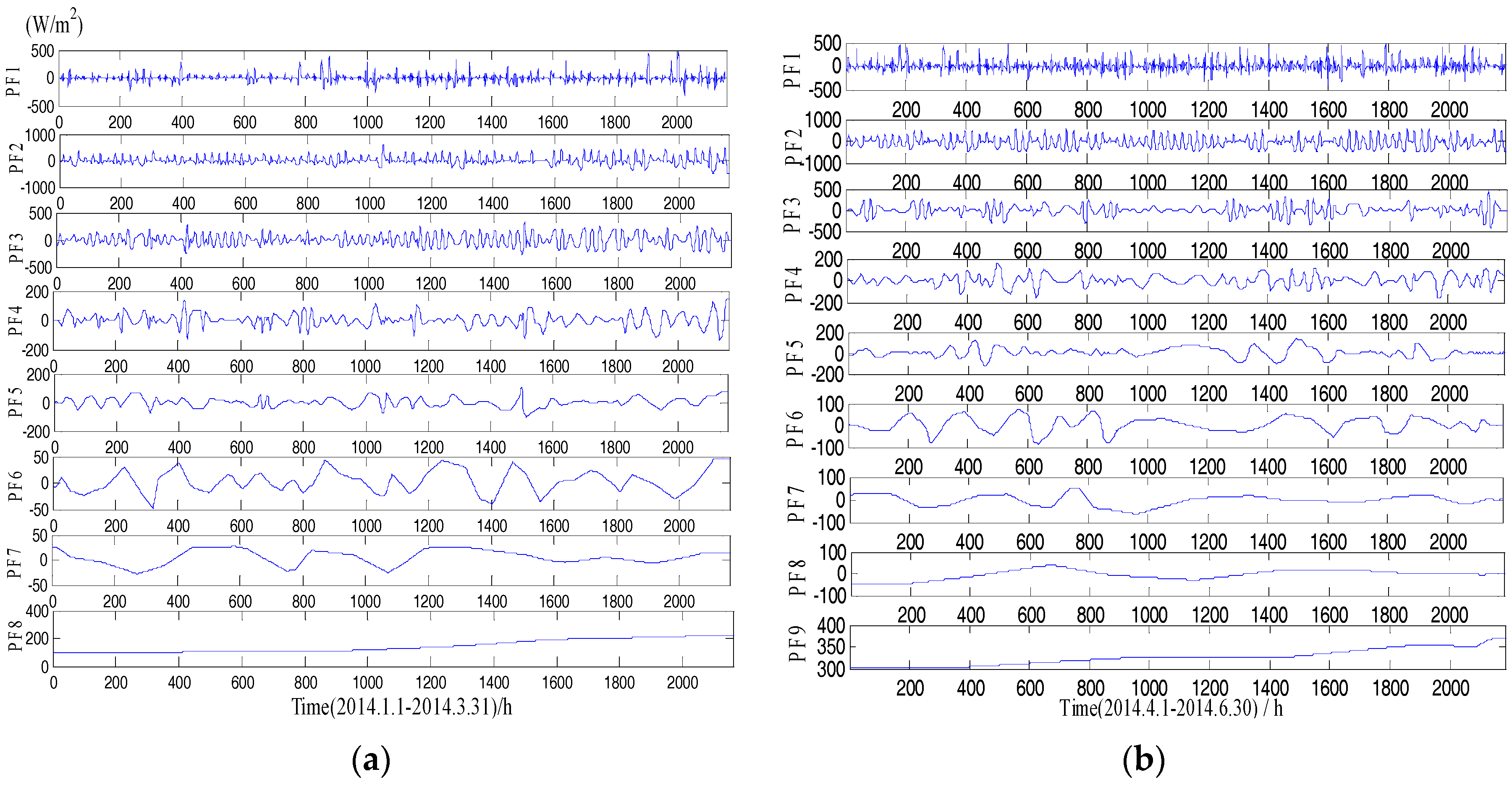
Figure 2 and Figure 3 show the different IMF and PF components decomposed from the original GHI series using the EMD and the LMD, respectively. As we can see, the original GHI series was decomposed into a set of IMF and PF with different frequency. The frequency of IMF or PF is reduced with the increase of decomposition levels of the original signal. Both high-frequency IMF (PF) and low-frequency IMF (PF) have weaker nonstationarity than the original solar radiation sequence, and they are helpful to develop more accurate forecasting models.
After decomposition, the LSSVM and the Volterra models were established for each IMF and PF component. Due to limited space, the forecasting results for each IMF and PF decomposed by two datasets (1 January to 31 March, 1 April to 30 June) are shown in Table 4 and Table 5, respectively. The embedding dimensions of m, the values of RMSE and MAE showed the decrease tendency with the increase of decomposition levels, which may be attributed to the fact that the low-frequency components are more stable than the high-frequency components, and the stable time series can more easily obtain high forecasting accuracy. Except for the first components (i.e., IMF1 and PF1), the LSSVM and the Volterra models achieved excellent forecasting results for other components, with correlation coefficients of more than 0.97. The lower correlation coefficients obtained by the first components were due to the fact that the first components have more nonstationary characteristics than other components, which will bring difficulties for developing an accurate forecasting model.
The Volterra model is a polynomial regression model. It easily falls into a local minimum of the parameter space and is inapplicable in cases where the underlying system exhibits a high degree of complexity [44]. The LSSVM transforms the nonlinear regression problem in a low dimensional space into a linear regression problem in a high dimension space by using kernel mapping technique, so it exhibits unique advantages in strong nonlinear regression [45]. The first components (i.e., IMF1 and PF1) obtained in this study have a strong randomness and large volatility; therefore, it can be found that the accuracy of the LSSSVM for the first components were better than that of the Volterra models.
For the remaining components, the R values of the Volterra model are more stable and higher than those of the LSSVM. Moreover, the RMSE and MAE values of the Volterra model for the test data are lower than that of the LSSVM in general. Thus, the Volterra model exhibits more accurate and stable performance than the LSSVM model for low-frequency components, which reflect the overall physical characteristics of the system. As such, the Volterra model can clearly describe the physical meaning of the system and accurately predict the continuous function [46].
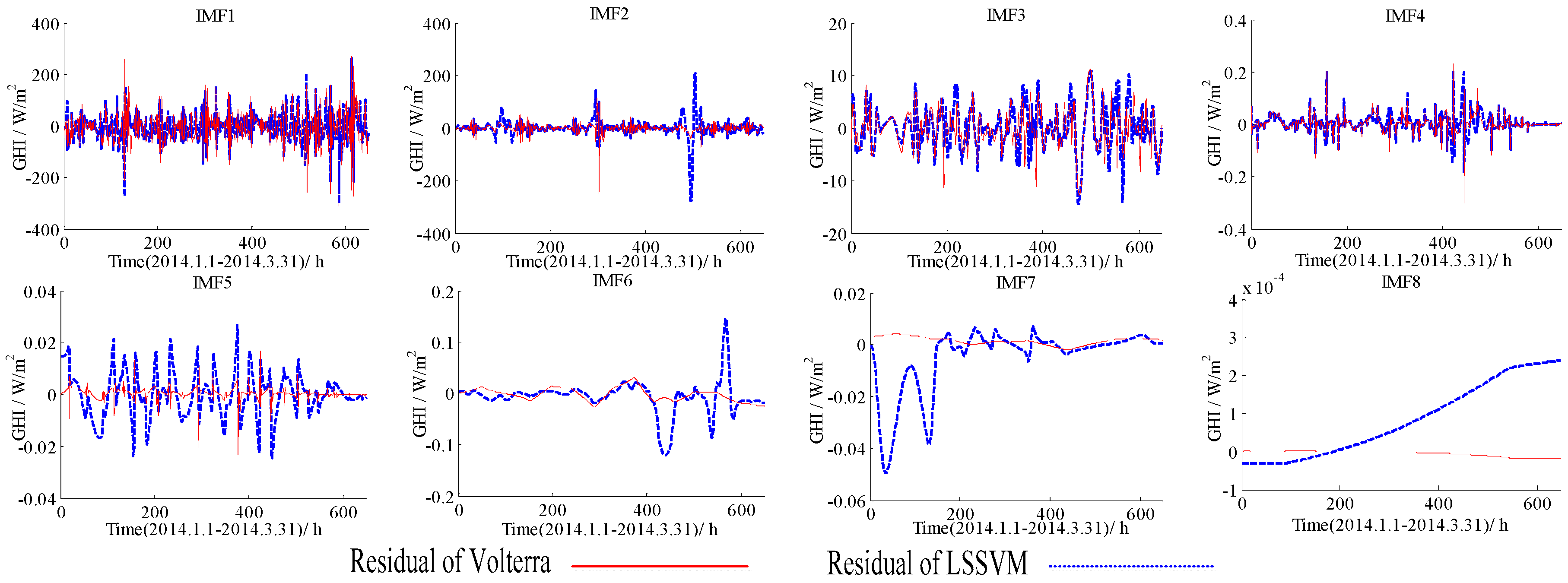
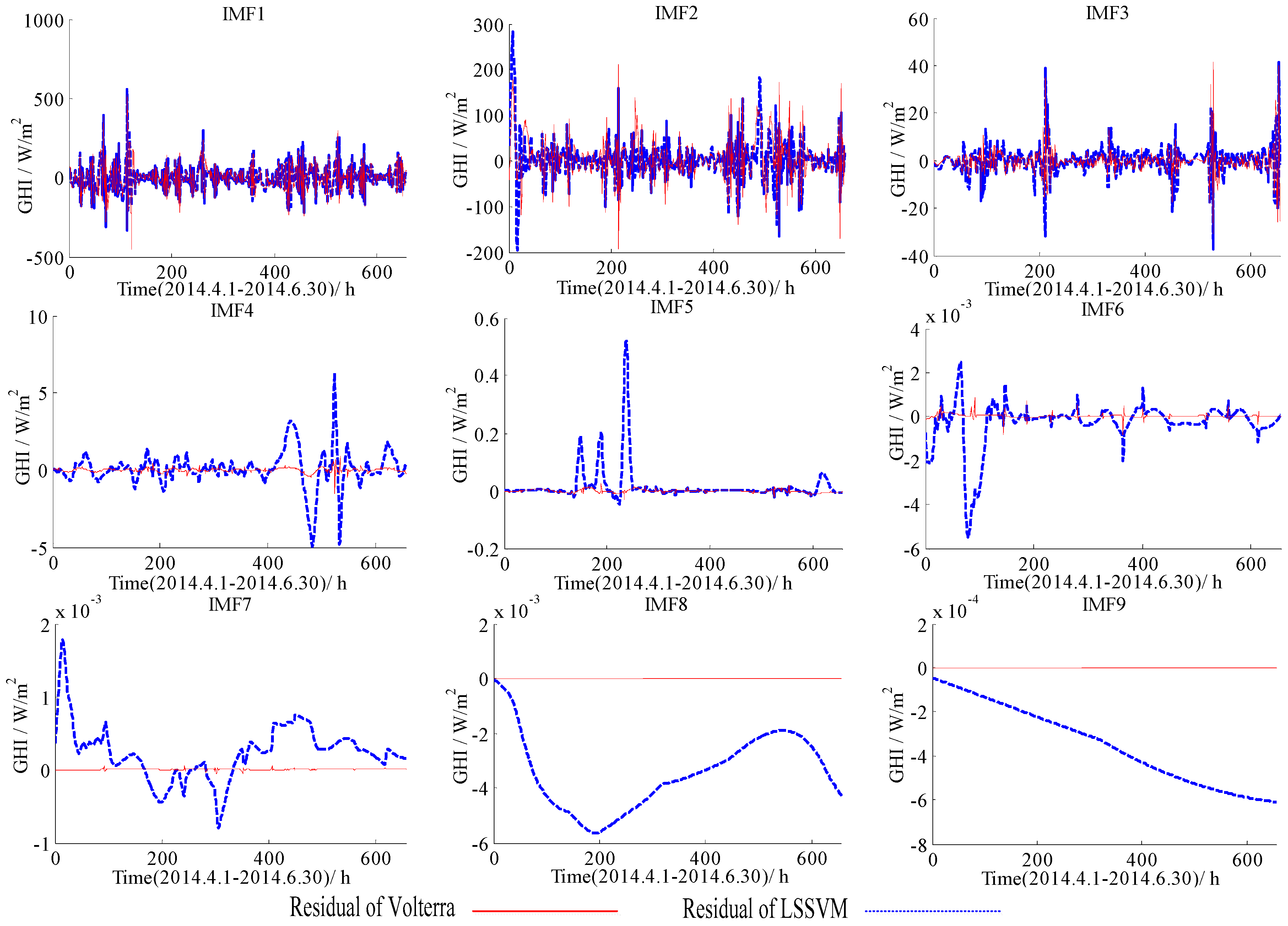
Forecasting residuals (i.e., forecasting results minus real value) with the LSSVM and the Volterra models for two datasets (1 January to 31 March, 1 April to 30 June) were shown in Figure 4, Figure 5, Figure 6 and Figure 7. Comparison clearly showed that the fitting residuals of the Volterra were smaller than the LSSVM for low-frequency components, while the fitting residuals of the LSSVM were smaller than Volterra for high-frequency components.
The final forecasting results for original GHI series, obtained by the different decomposition algorithms and modeling methods, were shown in Table 6. All of models based on the decomposition algorithm improved the forecasting results, compared to the LSSVM and the Volterra models without decomposition, meanwhile, the values of RMSE and forecast skill, obtained by these four models (EMD-LSSVM, LMD-LSSVM, EMD-Volterra, and LMD-Volterra), were significantly better than the persistence model for all the datasets. The results fully illustrated that using decomposition algorithm can effectively improve forecasting accuracies of GHI and model robustness.
5.3. The Forecasting Results for GHI Series Using the EMD-LSSVM-Volterra, the LMD-LSSVM-Volterra, and the EMD-LMD-LSSVM-Volterra Models
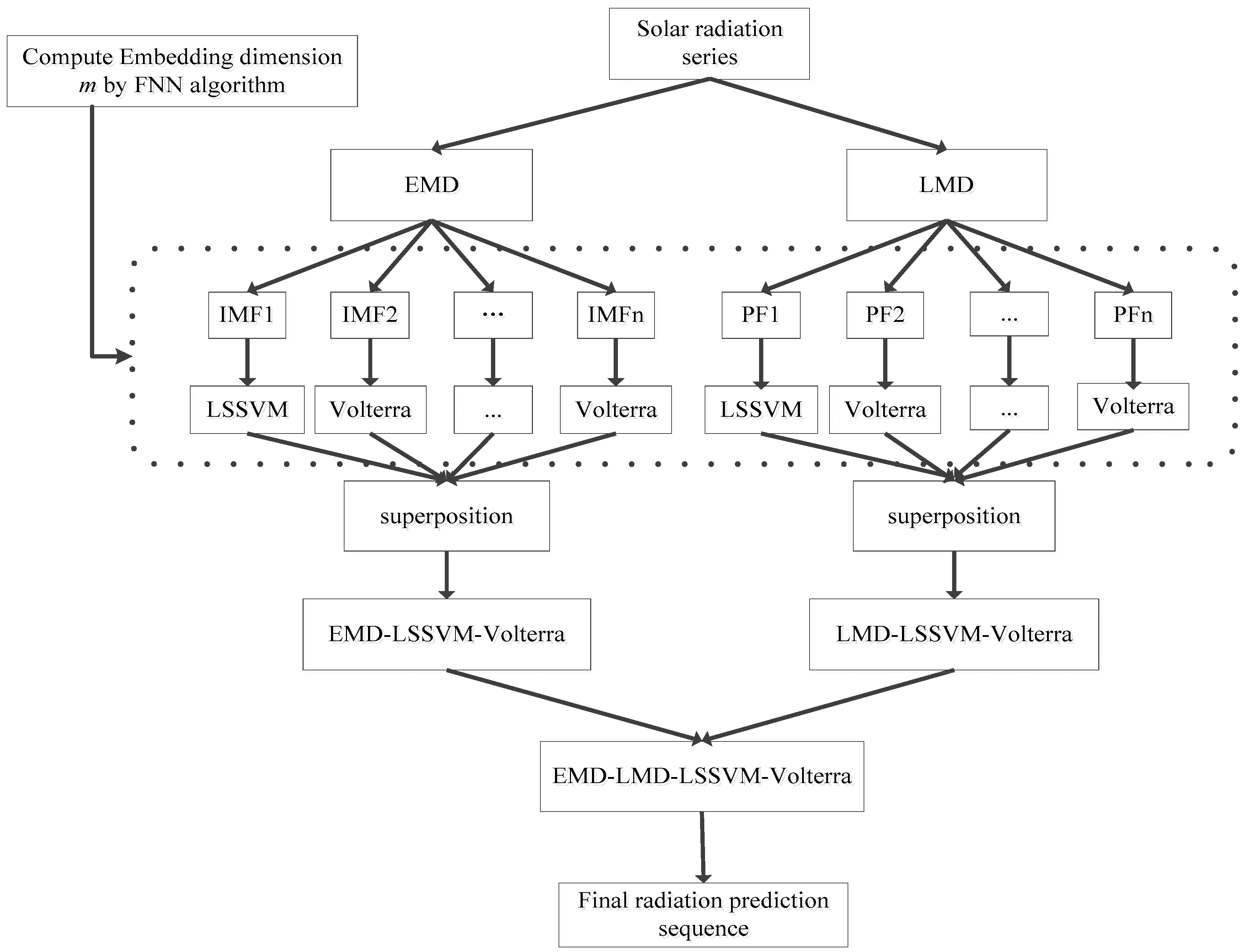
Analysis has shown that LSSVM is suitable for the high-frequency components (i.e., IMF1 and PF1) and the Volterra is suitable for the low-frequency components; the LSSVM and the Volterra models were combined to develop forecasting models (namely EMD-LSSVM-Volterra and LMD-LSSVM-Volterra, respectively). In other words, after signal decomposition by the EMD or LMD, the LSSVM was employed to develop a sub-model for the first components (i.e., IMF1 or PF1), while the Volterra was used to develop the sub-models for the remaining low-frequency components, and the final results were obtained by superposition of each sub-model. As shown in Table 7, the forecasting accuracies of the EMD-LSSVM-Volterra and the LMD-LSSVM-Volterra have various degrees of improvements for all the datasets, compared to the EMD-LSSVM, the LMD-LSSVM, the EMD-Volterra and the LMD-Volterra models. These differences are attributed to the fact that the EMD and the LMD have different explanatory power for the original signals. EMD presents several limitations in terms of end effect, over envelope, under envelope, and mode confusion. LMD, a new processing method for non-stationary signals, also exhibits obvious deficiencies compared with EMD. For example, the signal will be lagging behind or ahead of time when smoothing is performed for a long time, smoothing step cannot be optimally determined in the smoothing process, and no fast algorithm is available [38]. The signal in LMD smoothing easily advances or lags and EMD yields serious end effect; hence, we integrated both decomposition algorithms to deal with the original radiation series to improve the prediction accuracy. Therefore, in order to further improve the forecasting accuracy for GHI, a novel modeling method called EMD-LMD-LSSVM-Volterra was proposed in this study. The forecasting result obtained by the EMD-LMD-LSSVM-Volterra model is the average value of the EMD-LSSVM-Volterra model and the LMD-LSSVM-Volterra model. The entire process was shown in Figure 8, and comparison results were presented in Table 7.
The forecast skill values obtained by the EMD-LMD-LSSVM-Volterra models were improved by 11.37–32.48% and 10.94–115.03%, and the RMSE values were decreased by 5.92–13.83% and 9.61–20.79% for all the datasets, compared to the EMD-LSSVM-Volterra and the LMD-LSSVM-Volterra, respectively. Moreover, the values of MAE obtained by the EMD-LMD-LSSVM-Volterra model, which has a significant decrease compared to the EMD-LSSVM-Volterra model and the LMD-LSSVM-Volterra model, were also lower than that of the persistence models presented in Table 3. The correlation coefficient (R) values of the EMD-LMD-LSSVM-Volterra models achieved 0.974–0.986 for all the datasets, which indicates that the forecasting value has a strong correlation with the measured value of GHI. The ARIMA is a widely used modeling method for solar radiation forecasting, the results obtained by the ARIMA were also provided in Table 7. It can be easily found that the EMD-LMD-LSSVM-Volterra models were significantly better than the ARIMA models. Overall, the EMD-LMD-LSSVM-Volterra models achieved the best forecasting accuracy in terms of all the statistical parameters (RMSE, MAR, R, and Forecast Skill).
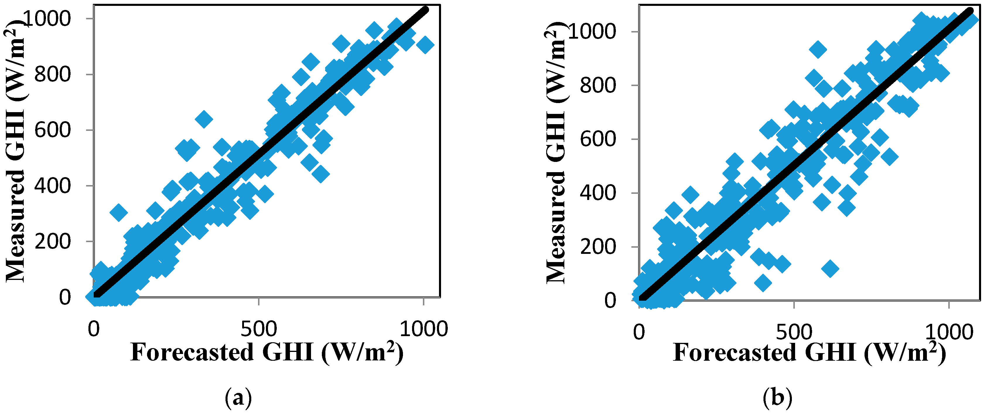
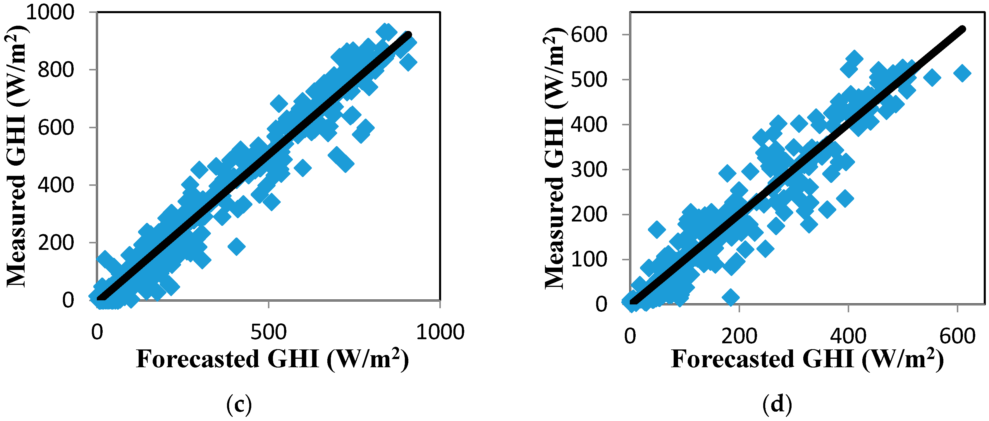
The correlation between the forecasted and measured values of GHI is plotted in Figure 9 to show the effectiveness of the forecasting approaches. The forecasted values of the EMD-LMD-LSSVM-Volterra model were strongly correlated with the measured GHI data.
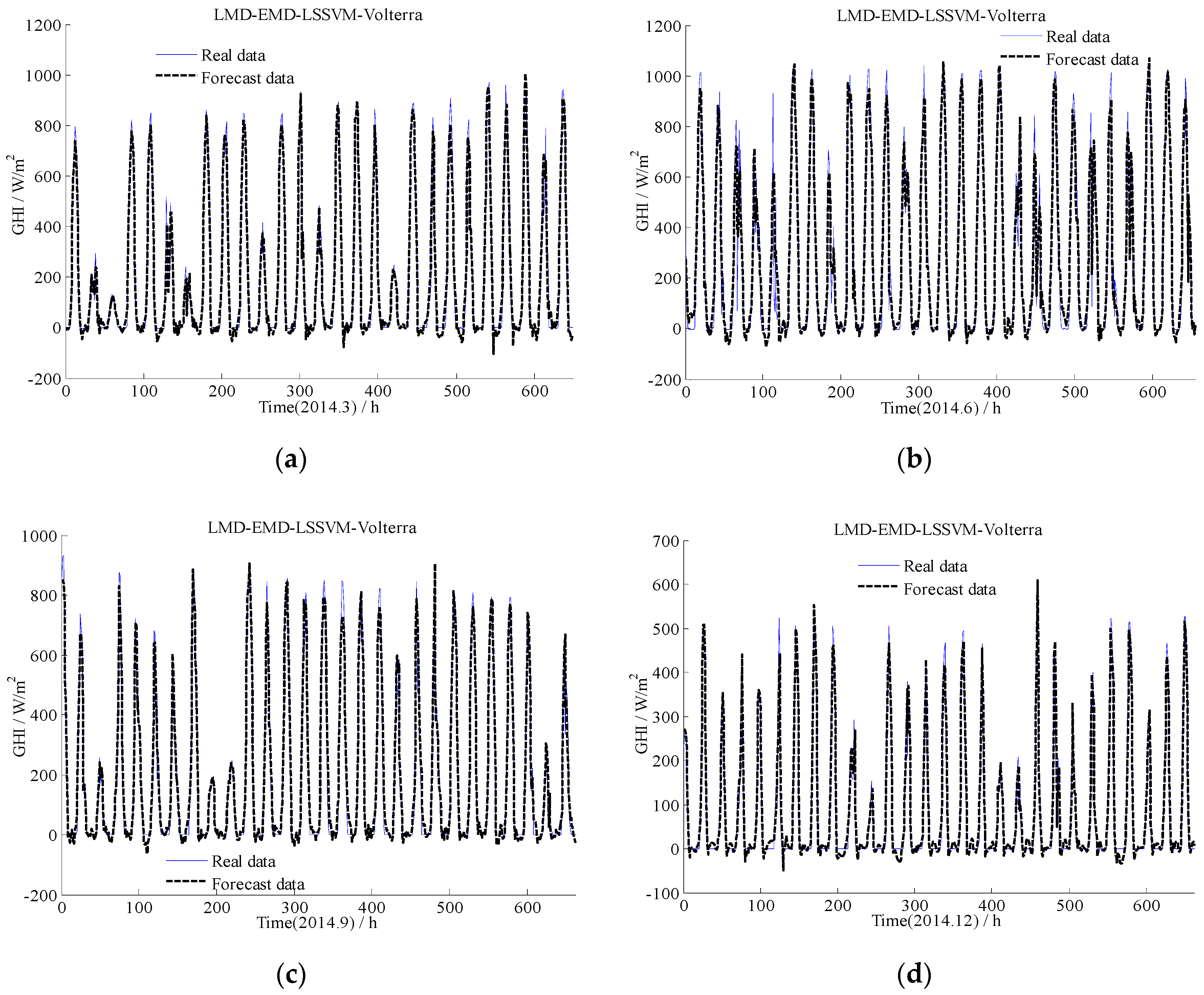
Figure 10 provided the comparison results of the EMD-LMD-LSSVM-Volterra method for hourly forecast. As shown in Figure 10, except night time periods (i.e., the band whose amplitude is close to 0), the proposed method can also forecast the variation trend of solar radiation. Notably, the EMD-LMD-LSSVM-Volterra model can forecast GHI in sunny days with high accuracy as well as in other weather conditions, even cloudy weather when solar radiation is less. The forecasted value of the model is consistent with the measured value. Compared with existing methods [47], the proposed method can be used without considering weather conditions and is thus considered effective for solar radiation forecasting.
5.4. The Forecasting Results for GHI Series Using the Persistence Model with Clear-Sky Index Forecasting under the ARIMA, the LSSVM, the Volterra, and the EMD-LMD-LSSVM-Volterra Models
The persistence model with clear-sky index is another widely used physical model for GHI forecasts. In this model, the clear-sky index has a great effect on the model accuracy. The clear-sky index time series not only contains the solar radiation information, but it also contains the information of other environmental physical quantities. Usually, the clear-sky index in time t + Δt was calculated based on actual solar radiation data and clear-sky radiation data in the time t (see Equation (20)). This is an approximate method which ignores the variation of the clear-sky index between the time t and t + Δt; hence, in order to obtain more accurate forecasting results obtained by persistence model, it is necessary to develop a forecasting model for the clear-sky index. In this study, the persistence model combined with the ARIMA, the LSSVM, the Volterra, and the EMD-LMD-LSSVM-Volterra model were also used for solar radiation forecast. Firstly, the clear-sky indexes k(t) are calculated through using measured values of solar radiation I(t) divided by the calculated values of the clear-sky solar radiation Iclr(t). Here, Iclr(t) were obtained based on the Bird model. Then the ARIMA, the LSSVM, the Volterra and the EMD-LMD-LSSVM-Volterra models were separately built to forecast the clear-sky index using historical data of k(t). Finally, the forecasted value of can be achieved using multiplied by the Iclr(t+1). The final results obtained by these methods were shown in Table 8. It also can be found that the EMD-LMD-LSSVM-Volterra models combined with persistence model gained the best performance compared with other three methods and had a similar performance with Table 7. In conclusion, the EMD-LM-LSSVM-Volterra models can accurately forecast solar radiation whether it’s only using original GHI series or based on the clear sky index series which contains enough information of environmental physical quantity.
6. Conclusions
A novel hybrid method combining EMD, LMD, LSSVM and Volterra algorithms was proposed as a statistical tool for forecasting hourly solar radiation only dependent on GHI series. The performance of the newly proposed models was checked on the gathered data from Golden, (CO, USA) and compared with the performance of the respective single and simple hybrid models. The main conclusions of this paper are summarized as follows: firstly, the EMD-LMD method effectively decomposes the original GHI series into a series of stable components for different frequencies which accurately reflect the original feature information. Secondly, different LSSVM and Volterra sub-models established according to the law of variation of these components can achieve the best results. Lastly, the EMD-LMD-LSSVM-Volterra model accurately forecasts the solar radiation whether it’s only using original GHI series or based on the clear sky index series.
A whole series of simulations validated the effectiveness of the proposed EMD-LMD-LSSVM-Volterra model on forecasting the complex and strongly nonlinear solar radiation time series. In the application stduies against a renewable energy background, we believe that this method can also effectively decompose and forecast other nonstationary time series signals, such as the wind speed series for wind power generation and energy load time series forecasting. In this study, only one-step forecasting (i.e., using current and previous radiation data to forecast solar radiation values in the next hour) was studied; the application effect of the proposed method in the long-term forecast of solar radiation is an issue that needs to be studied in the future. On the other hand, one year of data from one site was used in this study, further research is needed by including solar radiation data form more locations and under different sky conditions over a wider time period.
Acknowledgments
Authors thank National Renewable Energy Laboratory (NREL, URL link: http://www.nrel.gov/midc/srrl_bms/) for providing the solar radiation data. Funding: This work was supported by the national natural science foundation of China (grant numbers 61772240, 61775086), the fundamental research funds for the central universities (JUSRP51730A), the prospective joint research foundation of Jiangsu province of China (BY2016022-32), and sponsored by the 111 project (B12018).
Author Contributions
All the researchers were worked equally. Each of them helped in the writing of this paper and the design of the hybrid model and the simulations.
Conflicts of Interest
The authors declare no conflict of interest.
Nomenclature
| ANN | Artificial Neural Network |
| ARIMA | Autoregressive Integrated Moving Average |
| ARMA | Autoregressive Moving Average |
| EMD | Empirical Mode Decomposition |
| FNN | False Nearest Neighbor |
| GHI | Global Horizontal Irradiance |
| IMF | Intrinsic Mode Function |
| LMD | Local Mean Decomposition |
| LSSVM | Least Squares Support Vector Machine |
| SVM | Support Vector Machine |
| PF | Product Function |
| RH | Relative Humidity |
| R | Correlation Coefficient |
| RMSE | Root Mean Square Error |
| MAE | Mean Absolute Error |
References
- Lave, M.; Kleissl, J. Solar variability of four sites across the state of Colorado. Renew. Energy 2010, 35, 2867–2873. [Google Scholar] [CrossRef]
- Chi, W.C.; Urquhart, B.; Lave, M.; Dominguez, A.; Kleissl, J.; Shields, J.; Washom, B. Intra–hour forecasting with a total sky imager at the UC San Diego solar energy testbed. Sol. Energy 2011, 85, 2881–2893. [Google Scholar] [CrossRef]
- Perez, R.; Kivalov, S.; Schlemmer, J.; Hemker, K.; Renné, D.; Hoff, T.E. Validation of short and medium term operational solar radiation forecasts in the US. Sol. Energy 2010, 84, 2161–2172. [Google Scholar] [CrossRef]
- Wei, C. Predictions of surface solar radiation on tilted solar panels using machine learning models: A case study of Taiwan City, Taiwan. Energies 2017, 10, 1660. [Google Scholar] [CrossRef]
- Langella, R.; Proto, D.; Testa, A. Solar radiation forecasting, accounting for daily variability. Energies 2016, 9, 200. [Google Scholar] [CrossRef]
- Bracale, A.; Caramia, P.; Carpinelli, G.; Fazio, A.R.D.; Ferruzi, G. A Bayesian method for short-term probabilistic forecasting of photovoltaic Generation in Smart Grid Operation and Control. Energies 2013, 6, 733–747. [Google Scholar] [CrossRef]
- Voyant, C.; Muselli, M.; Paoli, C.; Nivet, M. Numerical weather prediction (NWP) and hybrid ARMA/ANN model to predict global radiation. Energy 2012, 39, 341–355. [Google Scholar] [CrossRef]
- Akarslan, E.; Hocaoğlu, F.O.; Edizkan, R. A novel M–D (multi–dimensional) linear prediction filter approach for hourly solar radiation forecasting. Energy 2014, 73, 978–986. [Google Scholar] [CrossRef]
- Yang, D.; Ye, Z.; Lim, L.H.I.; Dong, Z. Very short-term irradiance forecasting using the lasso. Sol. Energy 2015, 114, 314–326. [Google Scholar] [CrossRef]
- Notton, G.; Paoli, C.; Ivanova, L.; Vasileva, S.; Nivet, M.L. Neural network approach to estimate 10-min solar global irradiation values on tilted planes. Renew. Energy 2013, 50, 576–584. [Google Scholar] [CrossRef]
- Moghaddamnia, A.; Remesan, R.; Kashani, M.H.; Mohammadi, M.; Han, D.; Piri, J. Comparison of LLR, MLP, Elman, NNARX and ANFIS Models with a case study in solar radiation estimation. J. Atmos. Sol.-Terr. Phys. 2009, 71, 975–982. [Google Scholar] [CrossRef]
- Hocaoğlu, F.O. Stochastic approach for daily solar radiation modeling. Sol. Energy 2011, 85, 278–287. [Google Scholar] [CrossRef]
- Boata, R.S.; Gravila, P. Functional fuzzy approach for forecasting daily global solar irradiation. Atmos. Res. 2012, 112, 79–88. [Google Scholar] [CrossRef]
- Mecibah, M.S.; Boukelia, T.E.; Tahtah, R.; Gairaa, K. Introducing the best model for estimation the monthly mean daily global solar radiation on a horizontal surface (Case study: Algeria). Renew. Sustain. Energy Rev. 2014, 36, 194–202. [Google Scholar] [CrossRef]
- Wu, J.; Chan, C.K. Prediction of hourly solar radiation using a novel hybrid model of ARMA and TDNN. Sol. Energy 2011, 85, 808–817. [Google Scholar] [CrossRef]
- Alvanitopoulos, P.F.; Andreadis, I.; Georgoulas, N.; Zervakis, M.; Nikolaidis, N. Solar radiation prediction model based on Empirical Mode Decomposition. In Proceedings of the 2014 IEEE International Conference on Imaging Systems and Techniques (IST), Santorini, Greece, 14–17 October 2014; pp. 14–17. [Google Scholar] [CrossRef]
- Monjoly, S.; André, M.; Calif, R.; Soubdhan, T. Hourly forecasting of global solar radiation based on multiscale decomposition methods: A hybrid approach. Energy 2017, 119, 288–298. [Google Scholar] [CrossRef]
- Chicco, G.; Cocina, V.; Leo, P.D.; Spertino, F.; Pavan, A.M. Error Assessment of Solar Irradiance Forecasts and AC Power from Energy Conversion Model in Grid-Connected Photovoltaic Systems. Energies 2016, 9, 8. [Google Scholar] [CrossRef] [Green Version]
- Marquez, R.; Pedro, H.T.C.; Coimbra, C.F.M. Hybrid solar forecasting method uses satellite imaging and ground telemetry as inputs to ANNs. Sol. Energy 2013, 92, 176–188. [Google Scholar] [CrossRef]
- Brabec, M.; Paulescu, M.; Badescu, V. Tailored vs black-box models for forecasting hourly average solar irradiance. Sol. Energy 2015, 111, 320–331. [Google Scholar] [CrossRef]
- Paulescu, M.; Brabec, M.; Boata, R.; Badescu, V. Structured, physically inspired (gray box) models versus black box modeling for forecasting the output power of photovoltaic plants. Energy 2017, 121, 792–802. [Google Scholar] [CrossRef]
- Ghelardoni, L.; Ghio, A.; Anguita, D. Energy load forecasting using empirical mode decomposition and support vector regression. IEEE Trans. Smart Grid 2013, 4, 549–556. [Google Scholar] [CrossRef]
- Ren, Y.; Suganthan, P.N.; Srikanth, N. A comparative study of empirical mode decomposition–based short–term wind speed forecasting methods. IEEE Trans. Sustain. Energy 2015, 6, 236–244. [Google Scholar] [CrossRef]
- Park, C.; Looney, D.; Hulle, M.M.V.; Mandic, D.P. The complex local mean decomposition. Neurocomputing 2011, 74, 867–875. [Google Scholar] [CrossRef]
- Huang, N.E.; Shen, Z.; Long, S.R.; Wu, M.C.; Shih, H.H.; Zheng, Q.; Yen, N.C.; Tung, C.C.; Liu, H.H. The empirical mode decomposition and the hilbert spectrum for nonlinear and non–stationary time series analysis. Proc. Math. Phys. Eng. Sci. 1998, 454, 903–995. [Google Scholar] [CrossRef]
- Mookiah, M.R.K.; Achary, U.R.; Fujit, H.; Koh, J.E.W.; Tan, J.H.; Chu, C.K.; Bhandary, S.V.; Noronha, K.; Laude, A.; Tong, L. Automated detection of age-related macular degeneration using empirical mode decomposition. Knowl.-Based Syst. 2015, 89, 654–668. [Google Scholar] [CrossRef]
- Smith, J.S. The local mean decomposition and its application to EEG perception data. J. R. Soc. Interface 2005, 2, 443–454. [Google Scholar] [CrossRef] [PubMed]
- Kennel, M.B.; Brown, R.; Abarbanel, H.D.I. Determining embedding dimension for phase space reconstruction using a geometrical construction. Phys. Rev. A 1992, 45, 3403–3411. [Google Scholar] [CrossRef] [PubMed]
- Maheswaran, R.; Khosa, R. Wavelet Volterra Coupled Models for forecasting of nonlinear and non-stationary time series. Neurocomputing 2013, 149, 1074–1084. [Google Scholar] [CrossRef]
- Zhao, B.; Yong, L.; Xia, S.W. Support vector machine and its application in handwritten numeral recognition. Pattern Recognit. 2000, 2, 720–723. [Google Scholar] [CrossRef]
- Gharagheizi, F.; Ilani–Kashkouli, P.; Sattari, M.; Mohammadi, A.H.; Ramjugernath, D.; Richon, D. Development of a LSSVM–GC model for estimating the electrical conductivity of ionic liquids. Chem. Eng. Res. Des. 2014, 92, 66–79. [Google Scholar] [CrossRef]
- Gestel, T.V.; Suykens, J.A.K.; Baestaens, D.-E.; Lambrechts, A.; Lanckriet, G.; Vandaele, B.; Moor, B.D.; Vandewalle, J. Financial time series prediction using least squares support vector machines within the evidence framework. IEEE Trans. Neural Netw. 2001, 12, 809–821. [Google Scholar] [CrossRef] [PubMed]
- Suykens, J.A.K.; Vandewalle, J. Least squares support vector machine classifiers. Neural Process. Lett. 1999, 9, 293–300. [Google Scholar] [CrossRef]
- Ismail, S.; Shabri, A.; Samsudin, R. A hybrid model of self–organizing maps (SOM) and least square support vector machine (LSSVM) for time–series forecasting. Expert Syst. Appl. 2011, 38, 10574–10578. [Google Scholar] [CrossRef]
- Nowak, R.D.; Van, V.B.D. Random and pseudorandom inputs for Volterra filter identification. IEEE Trans. Signal Process. 1994, 42, 2124–2135. [Google Scholar] [CrossRef]
- Volterra, V. Theory of Functionals and of Integral and Integro–Differential Equations; Dover Publications: Mineola, NY, USA, 1959. [Google Scholar]
- Billings, S.A. Book review: The Volterra and Wiener theories of nonlinear systems. Int. J. Electr. Eng. Educ. 1980, 18, 187. [Google Scholar] [CrossRef]
- Pandey, C.K.; Katiyar, A.K. A note on diffuse solar radiation on a tilted surface. Energy 2009, 34, 1764–1769. [Google Scholar] [CrossRef]
- Zhao, N.; Zeng, X.; Han, S. Solar radiation estimation using sunshine hour and air pollution index in china. Energy Convers. Manag. 2013, 76, 846–851. [Google Scholar] [CrossRef]
- Elagib, N.A.; Alvi, S.H.; Mansell, M.G. Correlation ships between clearness index and relative sunshine duration for Sudan. Renew. Energy 1999, 17, 473–498. [Google Scholar] [CrossRef]
- Coimbra, C.F.M.; Kleissl, J.; Marquez, R. Overview of solar forecasting methods and a metric for accuracy evaluation. In Solar Energy Forecasting and Resource Assessment, 1st ed.; Kleissl, J., Ed.; Elsevier Academic Press: Boston, MA, USA, 2013; Chapter 8; pp. 171–194. ISBN 9780123971777. [Google Scholar]
- Marquez, R.; Coimbra, C.F.M. Proposed metric for evaluation of solar forecasting models. J. Sol. Energy Eng. 2011, 135, 011016. [Google Scholar] [CrossRef]
- Bird, R.E.; Hulstrom, R.L. A Simplified Clear Sky Model for Direct and Diffuse Insolation on Horizontal Surfaces; Technical Report; Solar Energy Research Institution: Golden, CO, USA, 1981. [Google Scholar]
- Dodd, T.J.; Wan, Y.; Drezet, P.; Harrison, R.F. Practical estimation of Volterra filters of arbitrary degree. Int. J. Control 2007, 80, 908–918. [Google Scholar] [CrossRef]
- Hwang, S.H.; Ham, D.H.; Kim, J.H. Forecasting performance of LS–SVM for nonlinear hydrological time series. KSCE J. Civ. Eng. 2012, 5, 870–882. [Google Scholar] [CrossRef]
- Zhu, A.; Pedro, J.C.; Brazil, T.J. Dynamic deviation reduction based Volterra behavioral modeling of RF power amplifiers. IEEE Trans. Microw. Theory Tech. 2006, 54, 4323–4332. [Google Scholar] [CrossRef]
- Chen, C.; Duan, S.; Cai, T.; Liu, B. Online 24-h solar power forecasting based on weather type classification using artificial neural network. Sol. Energy 2011, 85, 2856–2870. [Google Scholar] [CrossRef]
Figure 1.
The series of hourly GHI from 1 January 2014 to 31 December 2014 collected on Golden, Colorado.
Figure 1.
The series of hourly GHI from 1 January 2014 to 31 December 2014 collected on Golden, Colorado.

Figure 2.
Solar radiation sequence decomposition using EMD. (a) IMFs from Jan. to Mar.; (b) IMFs from Apr. to Jun.; (c) IMFs from Jul. to Sept.; (d) IMFs from Oct. to Dec.
Figure 2.
Solar radiation sequence decomposition using EMD. (a) IMFs from Jan. to Mar.; (b) IMFs from Apr. to Jun.; (c) IMFs from Jul. to Sept.; (d) IMFs from Oct. to Dec.
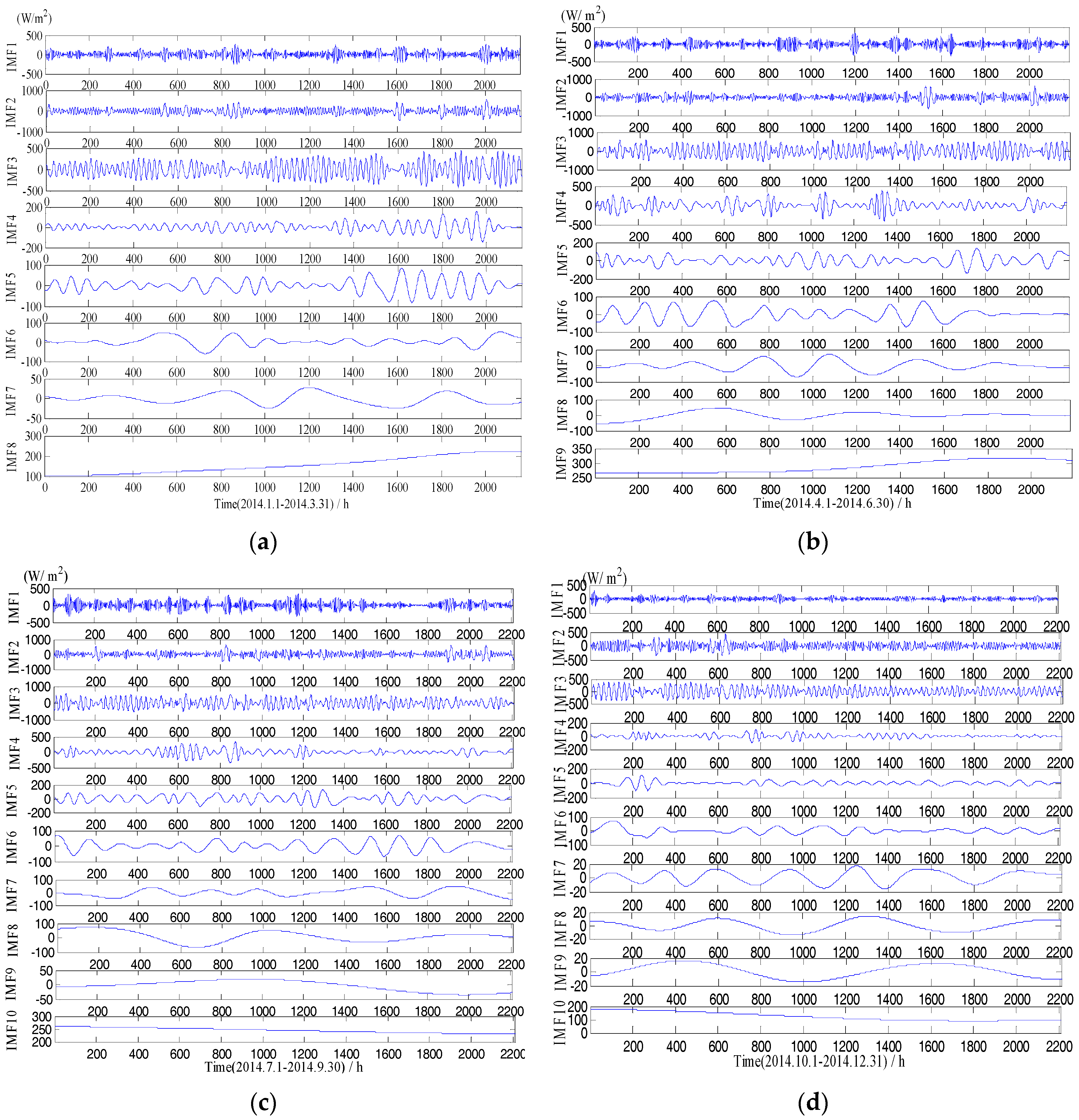
Figure 3.
Solar radiation sequence decomposition using the LMD. (a) PFs from Jan. to Mar.; (b) PFs from Apr. to Jun.; (c) PFs from Jul. to Sept.; (d) PFs from Oct. to Dec.
Figure 3.
Solar radiation sequence decomposition using the LMD. (a) PFs from Jan. to Mar.; (b) PFs from Apr. to Jun.; (c) PFs from Jul. to Sept.; (d) PFs from Oct. to Dec.

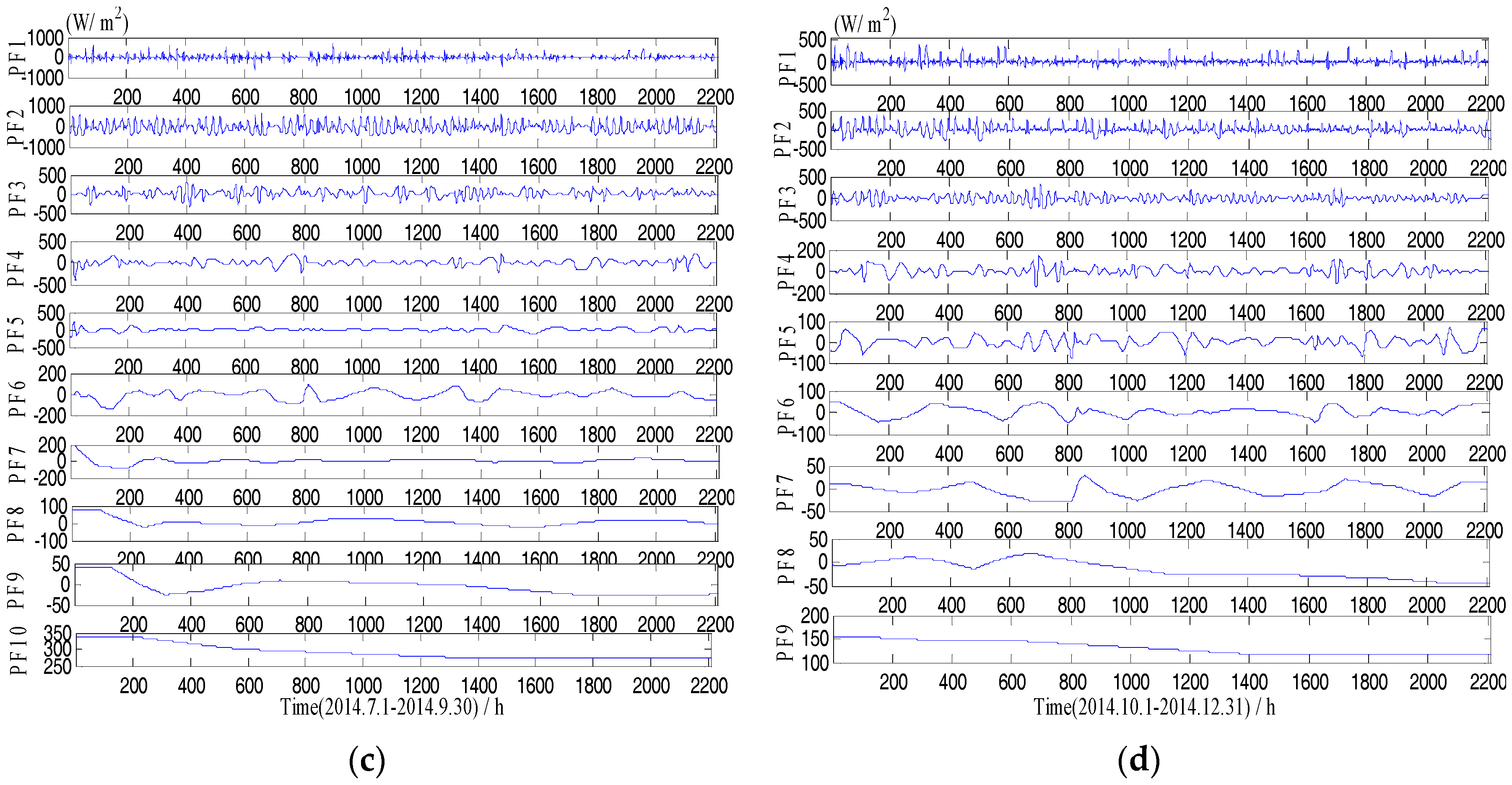
Figure 4.
Forecasting residuals of the LSSVM and the Volterra models with different IMFs based on the data of 1 January to 31 March in 2014.
Figure 4.
Forecasting residuals of the LSSVM and the Volterra models with different IMFs based on the data of 1 January to 31 March in 2014.

Figure 5.
Forecasting residuals of the LSSVM and the Volterra models with different PFs based on the data of 1 January to 31 March in 2014.
Figure 5.
Forecasting residuals of the LSSVM and the Volterra models with different PFs based on the data of 1 January to 31 March in 2014.
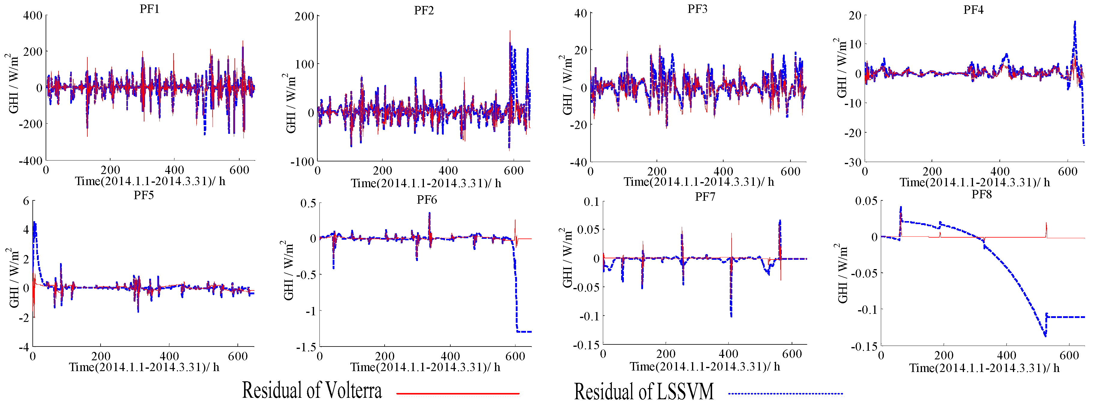
Figure 6.
Forecasting residuals of the LSSVM and the Volterra models with different IMFs based on the data of 1 April to 30 June in 2014.
Figure 6.
Forecasting residuals of the LSSVM and the Volterra models with different IMFs based on the data of 1 April to 30 June in 2014.

Figure 7.
Forecasting residuals of the LSSVM and the Volterra models with different PFs based on the data of 1 April to 30 June in 2014.
Figure 7.
Forecasting residuals of the LSSVM and the Volterra models with different PFs based on the data of 1 April to 30 June in 2014.
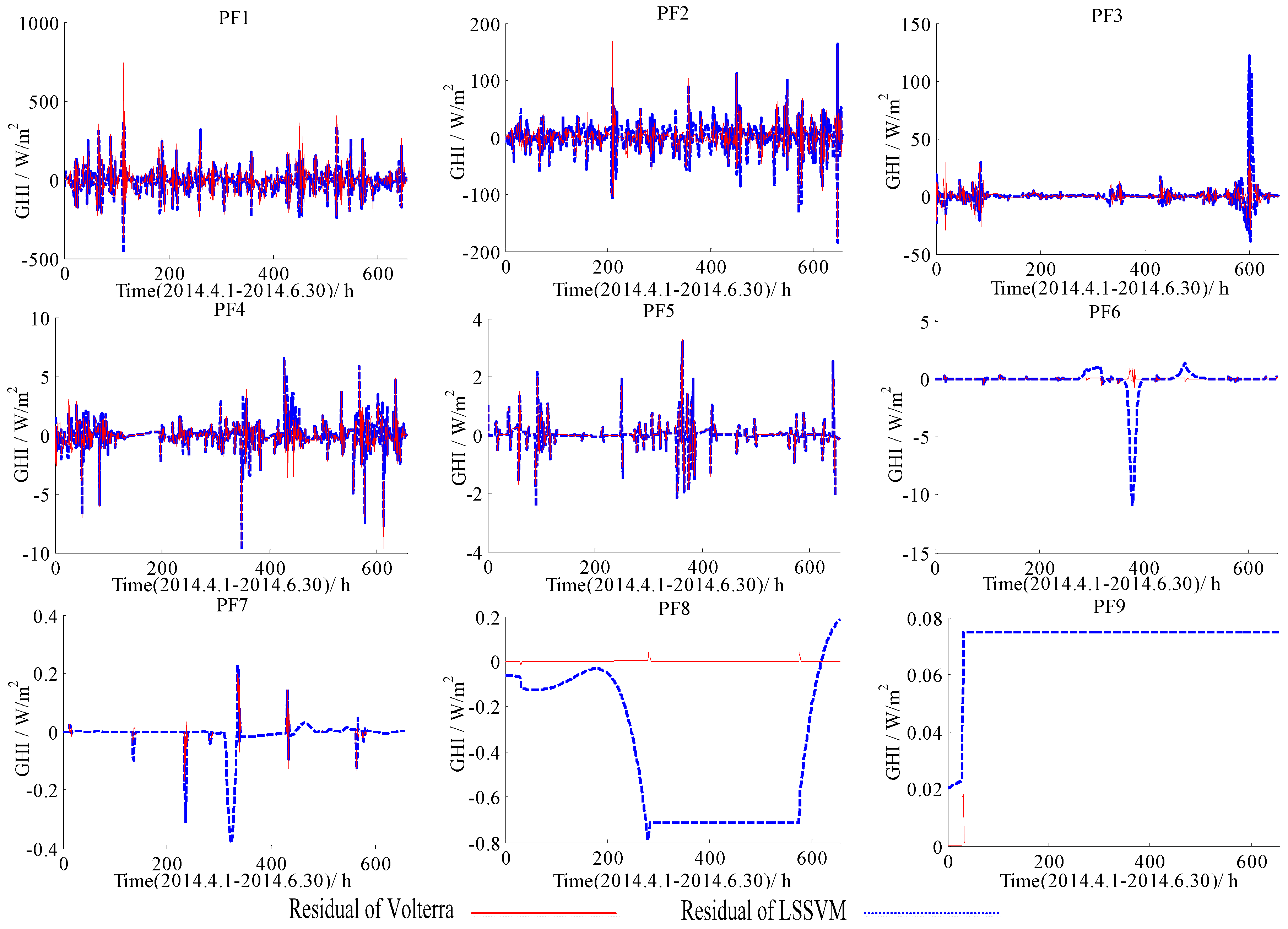
Figure 8.
Flow chart of developing the EMD-LMD-LSSVM-Volterra model for GHI forecast.

Figure 9.
Scatter plot of measured and forecasted GHI for the EMD-LMD-LSSVM-Volterra model. Black solid lines mark the identity (1:1) line. (a) Jan. to Mar.; (b) Apr. to Jun.; (c) Jul. to Sept.; (d) Oct. to Dec.
Figure 9.
Scatter plot of measured and forecasted GHI for the EMD-LMD-LSSVM-Volterra model. Black solid lines mark the identity (1:1) line. (a) Jan. to Mar.; (b) Apr. to Jun.; (c) Jul. to Sept.; (d) Oct. to Dec.


Figure 10.
Comparison between the measured and calculated values of hourly solar radiation through the EMD-LMD-LSSVM-Volterra model. (a) Jan. to Mar.; (b) Apr. to Jun.; (c) Jul. to Sept.; (d) Oct. to Dec.
Figure 10.
Comparison between the measured and calculated values of hourly solar radiation through the EMD-LMD-LSSVM-Volterra model. (a) Jan. to Mar.; (b) Apr. to Jun.; (c) Jul. to Sept.; (d) Oct. to Dec.


Table 1.
Environmental information about temperatures and relative humidity (RH) of the observation site in 2014.
Table 1.
Environmental information about temperatures and relative humidity (RH) of the observation site in 2014.
| Month | Avg Temp (°C) | Max Temp (°C) | Min Temp (°C) | Avg RH (%) | Max RH (%) | Min RH (%) |
|---|---|---|---|---|---|---|
| Jan. | 2.06 | 16.8 | −18.0 | 44.7 | 103 | 3.40 |
| Feb. | −0.61 | 17.9 | −25.1 | 57.5 | 105 | 5.60 |
| Mar. | 5.16 | 21.9 | −15.6 | 43.6 | 107 | 6.20 |
| Apr. | 9.29 | 15.9 | 2.76 | 42.9 | 70.6 | 21.6 |
| May | 13.4 | 19.9 | 7.51 | 53.7 | 79.0 | 31.7 |
| Jun. | 19.1 | 26.6 | 12.1 | 44.5 | 75.0 | 21.5 |
| Jul. | 22.3 | 29.1 | 16.7 | 48.3 | 75.0 | 28.2 |
| Aug. | 20.6 | 27.3 | 15.3 | 46.5 | 70.4 | 26.0 |
| Sept. | 17.8 | 24.48 | 11.98 | 51.58 | 76.18 | 29.6 |
| Oct. | 13.5 | 20.1 | 7.29 | 39.9 | 63.6 | 22.5 |
| Nov. | 3.56 | 10.6 | −3.00 | 45.0 | 69.8 | 25.9 |
| Dec. | 1.39 | 7.57 | −3.82 | 47.5 | 67.5 | 25.9 |
Table 2.
Input atmospheric parameters values of the Bird clear sky model.
| Lat | Long | TZ | Pressure mB | Ozone cm | H2O cm | AOD@ 500 nm | AOD@ 380 nm | Taua | Ba | Albedo |
|---|---|---|---|---|---|---|---|---|---|---|
| 40 | −105 | −7 | 840 | 0.3 | 1.5 | 0.1 | 0.15 | 0.08 | 0.85 | 0.2 |
Table 3.
The performance comparison of the persistence, the LSSVM and the Volterra models for the four datasets.
Table 3.
The performance comparison of the persistence, the LSSVM and the Volterra models for the four datasets.
| Period | Models | RMSE (W/m2) | MAE (W/m2) | R | Forecast Skill |
|---|---|---|---|---|---|
| Jan. to Mar. | Persistence | 120 | 36.8 | 0.923 | 0.00 |
| LSSVM | 74.0 | 46.6 | 0.975 | 38.3% | |
| Volterra | 88.1 | 56.0 | 0.963 | 26.6% | |
| Apr. to Jun. | Persistence | 121 | 55.4 | 0.941 | 0.00 |
| LSSVM | 110 | 62.1 | 0.948 | 9.09% | |
| Volterra | 118 | 73.2 | 0.939 | 2.48% | |
| Jul. to Sept. | Persistence | 68.7 | 30.1 | 0.970 | 0.00 |
| LSSVM | 76.9 | 50.8 | 0.962 | −11.9% | |
| Volterra | 75.7 | 49.4 | 0.962 | −10.2% | |
| Oct. to Dec. | Persistence | 74.3 | 24.5 | 0.890 | 0.00 |
| LSSVM | 46.0 | 25.6 | 0.957 | 38.1% | |
| Volterra | 44.5 | 25.8 | 0.954 | 40.1% |
Table 4.
The forecasting results of the LSSVM and the Volterra models for each component obtained by the EMD and the LMD based on the data of 1 January to 31 March in 2014.
Table 4.
The forecasting results of the LSSVM and the Volterra models for each component obtained by the EMD and the LMD based on the data of 1 January to 31 March in 2014.
| Components | m | LSSVM | Volterra | ||||
|---|---|---|---|---|---|---|---|
| RMSE (W/m2) | MAE (W/m2) | R | RMSE (W/m2) | MAE (W/m2) | R | ||
| IMF1 | 17 | 52.8 | 37.98 | 0.778 | 60.4 | 43.8 | 0.709 |
| IMF2 | 13 | 36.2 | 17.1 | 0.977 | 19.5 | 11.1 | 0.993 |
| IMF3 | 6 | 1.93 | 1.20 | 1.00 | 1.05 | 0.730 | 1.00 |
| IMF4 | 6 | 3.45 × 10⁻² | 2.06 × 10⁻² | 1.00 | 3.20 × 10⁻² | 1.86 × 10⁻² | 1.00 |
| IMF5 | 6 | 8.57 × 10⁻³ | 6.56 × 10⁻³ | 1.00 | 2.45 × 10⁻³ | 1.38 × 10⁻³ | 1.00 |
| IMF6 | 2 | 3.34 × 10⁻² | 1.80 × 10⁻² | 1.00 | 1.26 × 10⁻² | 1.03 × 10⁻² | 1.00 |
| IMF7 | 2 | 1.35 × 10⁻² | 7.00 × 10⁻³ | 1.00 | 2.11 × 10⁻³ | 1.81 × 10⁻³ | 1.00 |
| IMF8 | 3 | 1.27 × 10⁻⁴ | 9.66 × 10⁻⁵ | 1.00 | 8.64 × 10⁻⁶ | 5.46 × 10⁻⁶ | 1.00 |
| PF1 | 10 | 52.7 | 32.0 | 0.716 | 55.7 | 33.8 | 0.675 |
| PF2 | 7 | 24.4 | 14.7 | 0.993 | 20.4 | 12.9 | 0.995 |
| PF3 | 6 | 5.90 | 4.38 | 1.00 | 5.73 | 4.17 | 1.00 |
| PF4 | 7 | 2.62 | 1.32 | 0.999 | 1.28 | 0.922 | 1.00 |
| PF5 | 6 | 0.576 | 0.207 | 1.00 | 0.255 | 0.157 | 1.00 |
| PF6 | 7 | 0.347 | 0.116 | 1.00 | 3.54 × 10⁻² | 1.74 × 10⁻² | 1.00 |
| PF7 | 4 | 1.07 × 10⁻² | 4.45 × 10⁻³ | 1.00 | 6.15 × 10⁻³ | 1.70 × 10⁻³ | 1.00 |
| PF8 | 2 | 6.38 × 10⁻² | 4.59 × 10⁻² | 1.00 | 2.66 × 10⁻³ | 1.38 × 10⁻³ | 1.00 |
Table 5.
The forecasting results of the LSSVM and the Volterra models for each component obtained by the EMD and the LMD based on the data of 1 April to 30 June in 2014.
Table 5.
The forecasting results of the LSSVM and the Volterra models for each component obtained by the EMD and the LMD based on the data of 1 April to 30 June in 2014.
| Components | m | LSSVM | Volterra | ||||
|---|---|---|---|---|---|---|---|
| RMSE (W/m2) | MAE (W/m2) | R | RMSE (W/m2) | MAE (W/m2) | R | ||
| IMF1 | 17 | 81.1 | 57.2 | 0.449 | 87.8 | 63.3 | 0.387 |
| IMF2 | 10 | 47.0 | 27.9 | 0.969 | 46.2 | 31.3 | 0.970 |
| IMF3 | 10 | 5.90 | 3.63 | 1.00 | 5.23 | 2.79 | 1.00 |
| IMF4 | 5 | 1.17 | 0.690 | 1.00 | 0.139 | 9.01 × 10⁻² | 1.00 |
| IMF5 | 5 | 6.74 × 10⁻² | 2.13 × 10⁻² | 1.00 | 5.69 × 10⁻³ | 5.69 × 10⁻³ | 1.00 |
| IMF6 | 5 | 1.07 × 10⁻³ | 5.49 × 10⁻⁴ | 1.00 | 1.08 × 10⁻⁴ | 5.77 × 10⁻⁵ | 1.00 |
| IMF7 | 6 | 4.44 × 10⁻⁴ | 3.45 × 10⁻⁴ | 1.00 | 6.67 × 10⁻⁶ | 2.95 × 10⁻⁶ | 1.00 |
| IMF8 | 4 | 3.69 × 10⁻³ | 3.42 × 10⁻³ | 1.00 | 2.17 × 10⁻⁷ | 1.33 × 10⁻⁷ | 1.00 |
| IMF9 | 4 | 3.90 × 10⁻⁴ | 3.47 × 10⁻⁴ | 1.00 | 4.65 × 10⁻⁷ | 3.71 × 10⁻⁷ | 1.00 |
| PF1 | 16 | 79.8 | 52.8 | 0.623 | 92.6 | 61.9 | 0.469 |
| PF2 | 6 | 25.9 | 17.1 | 0.995 | 24.6 | 14.9 | 0.996 |
| PF3 | 7 | 9.19 | 3.06 | 0.997 | 5.22 | 2.73 | 1.00 |
| PF4 | 7 | 1.25 | 0.717 | 1.00 | 1.23 | 0.717 | 1.00 |
| PF5 | 3 | 0.420 | 0.181 | 1.00 | 0.420 | 0.193 | 1.00 |
| PF6 | 4 | 1.28 | 0.320 | 1.00 | 0.103 | 4.11 × 10⁻² | 1.00 |
| PF7 | 4 | 5.60 × 10⁻² | 1.71 × 10⁻² | 1.00 | 1.92 × 10⁻² | 3.86 × 10⁻³ | 1.00 |
| PF8 | 2 | 0.508 | 0.409 | 1.00 | 4.04 × 10⁻³ | 1.43 × 10⁻³ | 1.00 |
| PF9 | 2 | 7.31 × 10⁻² | 7.22 × 10⁻² | 1.00 | 1.44 × 10⁻³ | 8.76 × 10⁻⁴ | 1.00 |
Table 6.
The forecasting results of the EMD-LSSVM, the LMD-LSSVM, the EMD-Volterra, and the LMD-Volterra for the four datasets in 2014.
Table 6.
The forecasting results of the EMD-LSSVM, the LMD-LSSVM, the EMD-Volterra, and the LMD-Volterra for the four datasets in 2014.
| Period | Models | RMSE (W/m2) | MAE (W/m2) | R | Forecast Skill |
|---|---|---|---|---|---|
| Jan. to Mar. | EMD-LSSVM | 62.6 | 42.8 | 0.977 | 47.8% |
| EMD-Volterra | 64.8 | 45.9 | 0.976 | 46.0% | |
| LMD-LSSVM | 58.4 | 37.4 | 0.981 | 51.3% | |
| LMD-Volterra | 60.0 | 37.8 | 0.979 | 50.0% | |
| Apr. to Jun. | EMD-LSSVM | 89.9 | 62.8 | 0.965 | 25.7% |
| EMD-Volterra | 90.3 | 63.6 | 0.965 | 25.4% | |
| LMD-LSSVM | 85.8 | 58.3 | 0.968 | 29.1% | |
| LMD-Volterra | 98.0 | 66.3 | 0.958 | 19.0% | |
| Jul. to Sept. | EMD-LSSVM | 51.6 | 35.6 | 0.982 | 24.9% |
| EMD-Volterra | 60.7 | 45.2 | 0.975 | 11.6% | |
| LMD-LSSVM | 58.8 | 39.9 | 0.977 | 14.4% | |
| LMD-Volterra | 66.4 | 42.6 | 0.971 | 3.35% | |
| Oct. to Dec. | EMD-LSSVM | 37.8 | 26.4 | 0.968 | 49.1% |
| EMD-Volterra | 38.0 | 28.3 | 0.967 | 48.9% | |
| LMD-LSSVM | 36.9 | 21.7 | 0.969 | 50.3% | |
| LMD-Volterra | 41.6 | 25.0 | 0.960 | 44.0% |
Table 7.
The forecasting accuracy comparisons of the ARIMA, the EMD-LSSVM-Volterra, the LMD-LSSVM-Volterra, and the EMD-LMD-LSSVM-Volterra model.
Table 7.
The forecasting accuracy comparisons of the ARIMA, the EMD-LSSVM-Volterra, the LMD-LSSVM-Volterra, and the EMD-LMD-LSSVM-Volterra model.
| Period | Models | RMSE (W/m2) | MAE (W/m2) | R | Forecast Skill |
|---|---|---|---|---|---|
| Jan. to Mar. | ARIMA | 70.8 | 45.8 | 0.970 | 41.0% |
| EMD-LSSVM-Volterra | 57.7 | 40.6 | 0.981 | 51.9% | |
| LMD-LSSVM-Volterra | 57.5 | 36.3 | 0.981 | 52.1% | |
| EMD-LMD-LSSVM-Volterra | 50.7 | 33.8 | 0.985 | 57.8% | |
| Apr. to Jun. | ARIMA | 116 | 67.8 | 0.941 | 4.13% |
| EMD-LSSVM-Volterra | 87.8 | 61.4 | 0.967 | 27.4% | |
| LMD-LSSVM-Volterra | 85.3 | 57.6 | 0.969 | 29.5% | |
| EMD-LMD-LSSVM-Volterra | 77.1 | 52.2 | 0.974 | 36.3% | |
| Jul. to Sept. | ARIMA | 77.0 | 47.4 | 0.959 | −12.1% |
| EMD-LSSVM-Volterra | 49.0 | 33.7 | 0.984 | 28.7% | |
| LMD-LSSVM-Volterra | 58.2 | 38.7 | 0.977 | 15.3% | |
| EMD-LMD-LSSVM-Volterra | 46.1 | 29.9 | 0.986 | 32.9% | |
| Oct. to Dec. | ARIMA | 46.2 | 31.5 | 0.950 | 37.8% |
| EMD-LSSVM-Volterra | 37.6 | 26.3 | 0.968 | 49.4% | |
| LMD-LSSVM-Volterra | 36.7 | 21.5 | 0.969 | 50.6% | |
| EMD-LMD-LSSVM-Volterra | 32.4 | 20.2 | 0.976 | 56.4% |
Table 8.
The forecasting accuracy comparisons of the persistence model combined with the ARIMA, the LSSVM, the Volterra, and the EMD-LMD-LSSVM-Volterra model.
Table 8.
The forecasting accuracy comparisons of the persistence model combined with the ARIMA, the LSSVM, the Volterra, and the EMD-LMD-LSSVM-Volterra model.
| Period | Models | RMSE (W/m2) | MAE (W/m2) | R | Forecast Skill |
|---|---|---|---|---|---|
| Jan. to Mar. | ARIMA | 81.8 | 46.1 | 0.961 | 31.8% |
| LSSVM | 90.5 | 46.5 | 0.954 | 24.6% | |
| Volterra | 88.4 | 46.8 | 0.956 | 26.3% | |
| EMD-LMD-LSSVM-Volterra | 54.3 | 26.5 | 0.984 | 54.8% | |
| Apr. to Jun. | ARIMA | 124 | 66.6 | 0.936 | −2.48% |
| LSSVM | 115 | 62.3 | 0.943 | 4.96% | |
| Volterra | 116 | 64.6 | 0.942 | 4.13% | |
| EMD-LMD-LSSVM-Volterra | 67.0 | 36.1 | 0.981 | 44.6% | |
| Jul. to Sept. | ARIMA | 83.4 | 44.1 | 0.952 | −21.4% |
| LSSVM | 72.0 | 38.3 | 0.967 | −4.80% | |
| Volterra | 73.1 | 40.6 | 0.969 | −6.40% | |
| EMD-LMD-LSSVM-Volterra | 52.8 | 28.5 | 0.982 | 23.1% | |
| Oct. to Dec. | ARIMA | 46.4 | 22.9 | 0.957 | 37.6% |
| LSSVM | 45.7 | 20.8 | 0.953 | 38.5% | |
| Volterra | 46.0 | 21.6 | 0.952 | 38.1% | |
| EMD-LMD-LSSVM-Volterra | 26.3 | 12.3 | 0.984 | 64.6% |
© 2018 by the authors. Licensee MDPI, Basel, Switzerland. This article is an open access article distributed under the terms and conditions of the Creative Commons Attribution (CC BY) license (http://creativecommons.org/licenses/by/4.0/).
Share and Cite
MDPI and ACS Style
Wang, Z.; Tian, C.; Zhu, Q.; Huang, M. Hourly Solar Radiation Forecasting Using a Volterra-Least Squares Support Vector Machine Model Combined with Signal Decomposition. Energies 2018, 11, 68. https://doi.org/10.3390/en11010068
AMA Style
Wang Z, Tian C, Zhu Q, Huang M. Hourly Solar Radiation Forecasting Using a Volterra-Least Squares Support Vector Machine Model Combined with Signal Decomposition. Energies. 2018; 11(1):68. https://doi.org/10.3390/en11010068
Chicago/Turabian StyleWang, Zhenyu, Cuixia Tian, Qibing Zhu, and Min Huang. 2018. "Hourly Solar Radiation Forecasting Using a Volterra-Least Squares Support Vector Machine Model Combined with Signal Decomposition" Energies 11, no. 1: 68. https://doi.org/10.3390/en11010068
Note that from the first issue of 2016, this journal uses article numbers instead of page numbers. See further details here.