Toward Development of a Stochastic Wake Model: Validation Using LES and Turbine Loads


1
Department of Civil, Architectural and Environmental Engineering, University of Texas at Austin, Austin, TX 78712, USA
2
National Renewable Energy Laboratory, Golden, CO 80303, USA
3
Department of Mechanical Engineering, University of New Mexico, Albuquerque, NM 87131, USA
*
Author to whom correspondence should be addressed.
Energies 2018, 11(1), 53; https://doi.org/10.3390/en11010053
Submission received: 27 October 2017
/
Revised: 8 December 2017
/
Accepted: 14 December 2017
/
Published: 28 December 2017
(This article belongs to the Special Issue Wind Turbine Loads and Wind Plant Performance)
Abstract
:Wind turbines within an array do not experience free-stream undisturbed flow fields. Rather, the flow fields on internal turbines are influenced by wakes generated by upwind unit and exhibit different dynamic characteristics relative to the free stream. The International Electrotechnical Commission (IEC) standard 61400-1 for the design of wind turbines only considers a deterministic wake model for the design of a wind plant. This study is focused on the development of a stochastic model for waked wind fields. First, high-fidelity physics-based waked wind velocity fields are generated using Large-Eddy Simulation (LES). Stochastic characteristics of these LES waked wind velocity field, including mean and turbulence components, are analyzed. Wake-related mean and turbulence field-related parameters are then estimated for use with a stochastic model, using Multivariate Multiple Linear Regression (MMLR) with the LES data. To validate the simulated wind fields based on the stochastic model, wind turbine tower and blade loads are generated using aeroelastic simulation for utility-scale wind turbine models and compared with those based directly on the LES inflow. The study’s overall objective is to offer efficient and validated stochastic approaches that are computationally tractable for assessing the performance and loads of turbines operating in wakes.
1. Introduction
In wind turbine arrays or wind plants, it is usually the case that not all the turbine units experience the free-stream wind velocity field. Instead, depending on wind direction, one or more units can be subjected to blockage, resulting in wind speed deficit and/or enhanced turbulence from operating in the wake of upwind units. Within a wake, interesting wind field physical features and dynamic as well as spatially varying characteristics are best modeled using computational fluid dynamics (CFD) tools such as large-eddy simulation (LES) [1,2,3]. In contrast, in design, wind field features are, for convenience and ease of use, explained and most efficiently simulated using stochastic techniques that rely on turbulence power spectra and coherence functions and accompanying mean wind fields. The advantage of stochastic simulation is that one can describe flow field features in an efficient way, such as by the use of Inverse Fast Fourier Transform (IFFT) procedures; also, the entire simulation procedure relies on only very few input quantities or parameters. This speed and efficiency is useful in engineering applications [4,5]. In today’s design standards, wakes are starting to be more realistically accounted for since the earliest studies [6]. For example, the Dynamic Wake Meandering (DWM) model allows for wake effects from neighboring turbines to be accounted for in fatigue and ultimate limit state assessments [7,8,9]. The DWM model allows physically meaningful wake-induced turbulence along with wake deficit and meandering to be included. For describing wakes, one could say that CFD/LES can represent the physics most realistically and approaches like the DWM model offer a less expensive alternative with some approximation of the physics; stochastic simulation of wakes, if it were possible, would be even more efficient but the physics of the wake would need to be described in the few parameters employed in the inputs that are used.
Can complex waked wind fields be simulated using engineering stochastic simulation tools? This study attempts to answer this question. First, we generate free-stream and waked wind velocity fields using LES and study characteristics of these fields. For the free stream, we perform a “precursor” atmospheric LES of realistic inflow representing neutral atmospheric stability. This precursor field is then used as input to a wake-generating actuator line turbine model [10]. The simulated wake mean and turbulence field is captured at vertical planes 5, 7, and 10 rotor diameters downwind of this turbine. We report on stochastic (mean and turbulence) parameters and features estimated from the LES free-stream and waked wind velocity fields; we also describe attempts to understand spatial and temporal features of the wake. Next, we employ a regression-based approach to represent parameters that characterize the free-stream and wake mean and turbulence fields. Finally, turbine loads computed directly from the LES-generated wind fields are compared with those generated using stochastic simulation of wind fields that rely on parameters predicted by the regression-based model. The procedure outlined is an initial attempt in a longer-term study that is seeking to develop a framework for modeling wakes and associated turbine loads using tractable and inexpensive engineering simulation tools as alternatives to CFD.
2. Simulation of Wind Velocity Fields using LES
The governing equations used to describe the atmospheric fluid motion are based on the incompressible Navier–Stokes formulation expanded upon an unstructured grid. The spatial discretization employs a second-order central difference scheme using the PISO algorithm [11] to march forward in time with second-order temporal accuracy. The Navier–Stokes equations are augmented by the Coriolis force term and account for buoyancy via the Boussinesq approximation [12]. The turbine wakes are generated by the aerodynamic body forces computed by the actuator line method [10]. The body forces consist of lift and drag forces that are obtained from a two-dimensional lookup table based on inputs including the angle of attack and the incoming wind velocity at each blade element discretized uniformly along the blade line. The Smagorinsky [13] closure is used for the sub-grid scale (SGS) model in which the SGS constant is fixed at 0.13. The computational grid is locally refined near the turbine blade and along its wake path with three levels of nested grid employed by successively dividing the cells by half of its original size and finally yielding an approximate total number of 35 million grid points. This numerical approach has successfully demonstrated an accurate prediction of power for an existing offshore wind farm [14]. Additional numerical details pertaining to these computations can be found in Churchfield et al. [15].
We generate the desired inflow field by first performing a precursor atmospheric LES. The computational domain size must be large enough to capture the largest important scales of interest. For neutral atmospheric stability, these largest important scales are on the order of a few kilometers. Accordingly, we use a domain extending 3 km in both horizontal directions and 1 km in the vertical direction (Figure 1). A uniform grid resolution of 10 m is used in each direction, resulting in a precursor mesh containing cells. We use periodic lateral boundary conditions; additionally, a driving pressure gradient body force term is applied such that a target horizontally-averaged velocity at a specified height is achieved. In the case discussed in this study, we drive the flow (with the wind out of the southwest) so as to achieve a velocity of around 8 m/s at a height of 80 m above the surface since we use a turbine with a hub height of 80 m for the wake generation. The mean wind speed of the generated field at that height is 8.12 m/s. The upper boundary of the domain is treated as a rigid stress-free lid while the lower surface is modeled as a flat rough wall. A wall shear stress boundary condition that uses the Monin-Obuhkov scaling law is applied at the lower surface (a no-slip condition would not be appropriate unless individual roughness elements are resolved, which is impossible with LES at such high Reynolds number and the current state of computing power).
The velocity field is initialized uniformly at 8 m/s with organized sinusoidal perturbations near the surface to initiate turbulence. The potential temperature is initialized uniformly at 300 K up to 700 m above the surface. Over the next 100 m, the temperature linearly increases by 8 K. From 800 m up to the upper surface, the temperature increases at a rate of 0.003 K/m. Since the flow is of neutral stability, a zero temperature flux is applied at the lower surface, while the upper boundary condition for temperature is modeled so as to maintain the initial gradient. The Coriolis force is selected to be representative of a typical mid-latitude region at N. The flow is simulated until it reaches a quasi-equilibrium state, which, for this flow, occurs after about 18,000 s.
Once the desired quasi-equilibrium state is reached, planes of velocity and temperature data from the precursor simulation coinciding with the inflow planes (south and west in this case) are saved at every time step. The full precursor flow field at 18,000 s is also saved. These saved planes and the full flow field are used in simulations of the wake.
For the simulation of the wake, a computational domain with the same size as that used for the precursor simulation is chosen and an actuator line turbine model is located at the center of the domain. The full precursor flow field is set up inside the domain to initialize the simulation and the saved precursor inflow planes are used at every time step. The outflow boundary conditions (north and east planes) for velocity and temperature in the simulation with the turbine are modeled by a zero normal gradient. The time duration of the simulation is 600 s. An actuator line model of a 1.5 MW wind turbine is used to generate the waked flow. The hub height and rotor diameter of the selected turbine are 80 m and 77 m, respectively. The actuator line model is assumed to rotate at a constant rate of 16 rpm from the beginning to the end of the wake simulation.
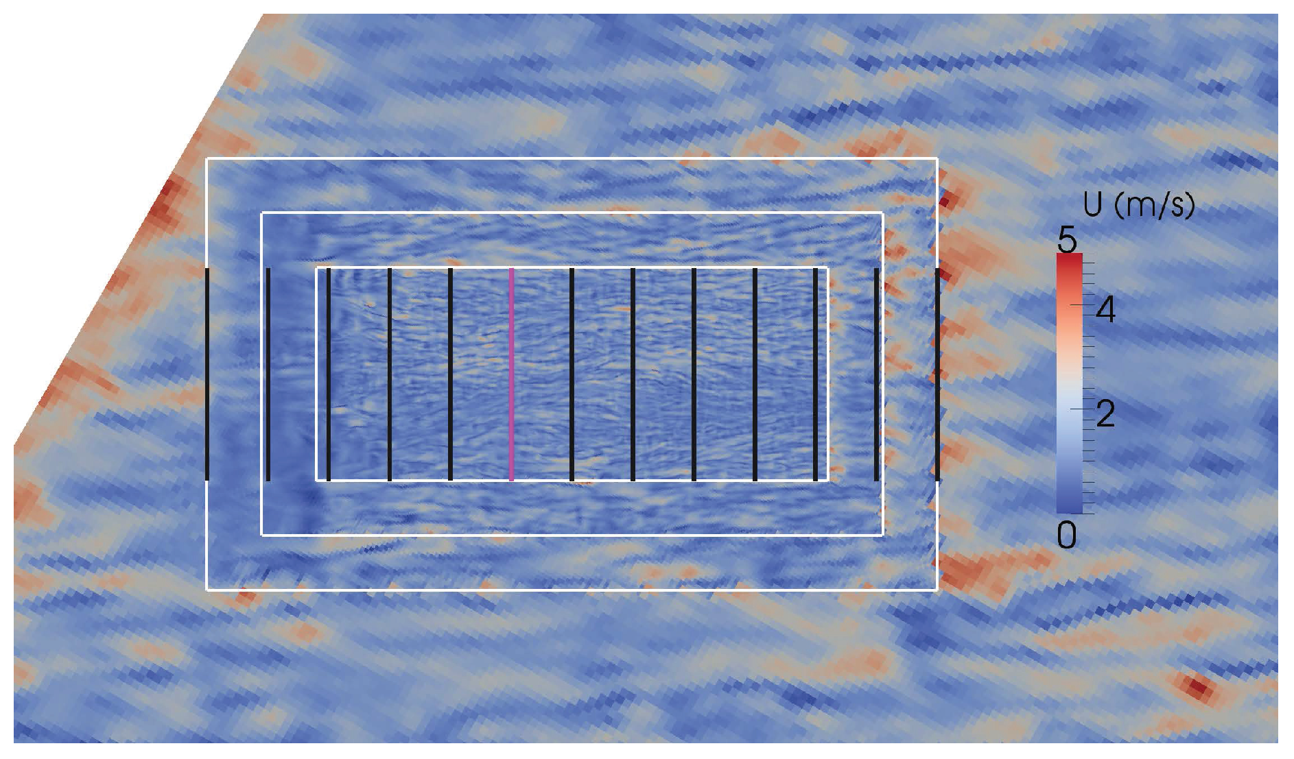
In contrast with the uniform mesh used for the precursor simulation, the mesh around the turbine is refined for the wake simulation to describe the interaction between the flow and the actuator line more accurately. Figure 2 shows a horizontal plane through the free-stream flow field that is taken near the surface ( m). Note that the computational grid is rotated because, in the simulation, the flow comes from an angle (out of the southwest); the plot is rotated as if the flow direction is from left to right. The magenta line shows the location of the wake-generating turbine, which is not simulated in this case. The white rectangles indicate outlines of the successively refined subdomains. The size of the cells located outside the largest subdomain is 10 m, the same as that of the precursor simulation; the size of cells at the innermost computational subdomain is 1.25 m (). The black lines shown are spaced one rotor diameter (D) apart from one another and from the magenta line. Total number of grid points are approximately 35 million.
Because we are interested in statistical and spectral characteristics of the wind velocity fields generated from LES, the effect of mesh refinement on these characteristics needs to be analyzed. To do this, we simulate the free stream using the same computational domain but with a refined mesh inside (still with no turbine). Inflow planes and the initial full flow field are also set up in the same way as for the wake simulation.
3. Statistical and Spectral Parameters
3.1. Free-Stream Wind Field Parameters
We discuss stochastic characteristics of the free-stream field, which represents the inflow field for the wake-generating turbine. The duration and sampling rate for the simulated free-stream time series studied are 600 s and 3.125 Hz, respectively. Figure 3 shows the variation in a vertical plane of the mean () and standard deviation () of the along-wind (), across-wind (), and vertical () wind velocity components at of the precursor domain (where the wake-generating turbine is to be located). The circles shown indicate where the turbine rotor is to be located for the wake simulation. In the figure, is seen to follow a vertical profile that is reasonable for neutral stability conditions. In addition, the component profile has a zero-mean, near-homogeneous spatial structure. The turbulence () plots suggest slight vertical variation for all three components, k. These mean and standard deviation profiles are all reasonable and suggest that the target atmospheric conditions are well described in the computational domain for the precursor.
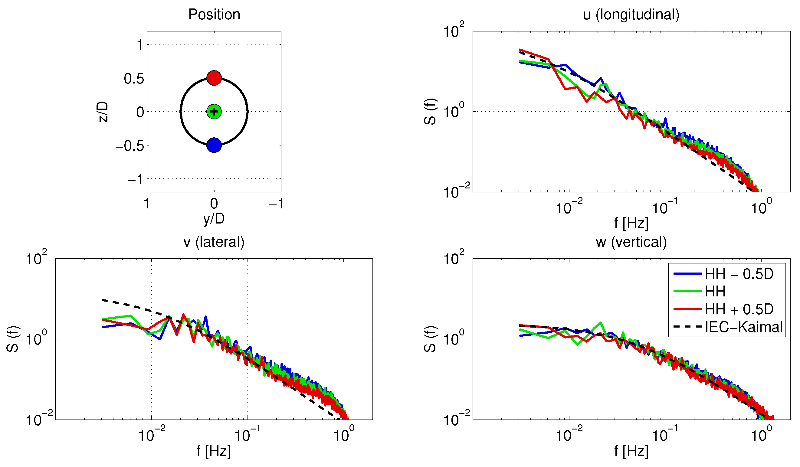
Figure 4 shows plots of the power spectral density (PSD) functions for the three free-stream turbulence components at different heights (top, center, and bottom of the rotor). The black dotted lines shown represent the Kaimal spectra specified in a design standard [16]; the power spectra for all the components closely resemble the Kaimal spectra over all frequencies. At high frequencies, around 0.8 Hz and greater, there are some differences that arise because LES has a limit, related to computational grid size, on resolving high-frequency energy. Although the LES sub-grid scale (SGS) model provides field energy at smaller scales in the simulations, a limit on resolving the smallest scales of energy is evident [17]. To assess the influence of grid size on free-stream turbulence spectra, it is useful to study Figure 5.
Figure 5 shows plots of power spectral density (PSD) functions for the three free-stream turbulence components at different downstream distances. Note that is where the wake-generating turbine will be located. Minus signs in the legend denote that these spectra are from velocity data captured at upstream locations relative to the wake-generating turbine. These free-stream fields are captured from the refined mesh and subdomains discussed in Section 2. In this figure, the high-frequency content in the PSD functions is seen to change with refinement of the mesh. At (where the mesh spacing is 5 m), the spectra of all the turbulence components begin to deviate from the constant −5/3 slope of the inertial subrange around 0.08 Hz; in contrast, at (where the mesh spacing is 1.25 m), the gradients of the spectra begin to deviated only around 0.8 Hz. This indicates that the grid or mesh refinement influences the high-frequency energy content in the spectra. Another interesting feature is that the high-frequency content increases from to , i.e., from coarser to finer grid refinement. LES-generated turbulence follows Kolmogorov’s theory on turbulence [18] and influences the high-frequency content in the spectra.
Figure 6 shows coherence functions for the three free-stream turbulence components with the same lateral separation at different elevations. The black dotted line for the longitudinal (u) component indicates an exponential coherence model used in a design standard [16]. Coherence functions for the v and w components, also discussed in a number of studies related to turbulence [19,20,21], are expectedly different from that for u. Coherence appears to depend on height; at lower heights, higher turbulence levels introduced by the lower boundary leads to weaker coherent in the wind field. The preceding observations related to statistical and spectral parameters all suggest that the simulated LES-generated free-stream wind field reflects characteristics of atmospheric turbulence satisfactorily.
3.2. Wake Wind Field Parameters
For analysis of the wake, we study wake velocity time series at vertical planes located at distances, , , and downwind of a wake-generating turbine. The duration and sampling rate for each wind time series are 600 s and 1 Hz, respectively. The actuator line is modeled as rotating counterclockwise. We discuss mean and standard deviation distributions of each turbulence component around the rotor plane of a turbine that could be located at the downwind planes. Power spectra of the three velocity components at different lateral and vertical positions are also presented. All these statistics and power spectra for the wake field are compared with those for the free-stream field. Because of insufficient data (only 600 samples) in the wake due to slower sampling relative to the free stream, coherence functions for the wake are not estimated.
Figure 7, Figure 8 and Figure 9 describe the spatial variation of in the free stream and at different downwind locations in the wake. Both the vertical plane variations and the vertical profile plots focus on areas centered on where a downwind turbine might be located. In Figure 7, the evolution and recovery of the mean wind speed deficit is evident around the rotor. The deficit around the rotor is combined with the mean wind profile of the free-stream field. This deficit is reduced as the flow moves downstream. At , around 83% of the free-stream mean wind speed is recovered at the hub. This recovery is consistent with findings from the study by Troldborg et al. [22].
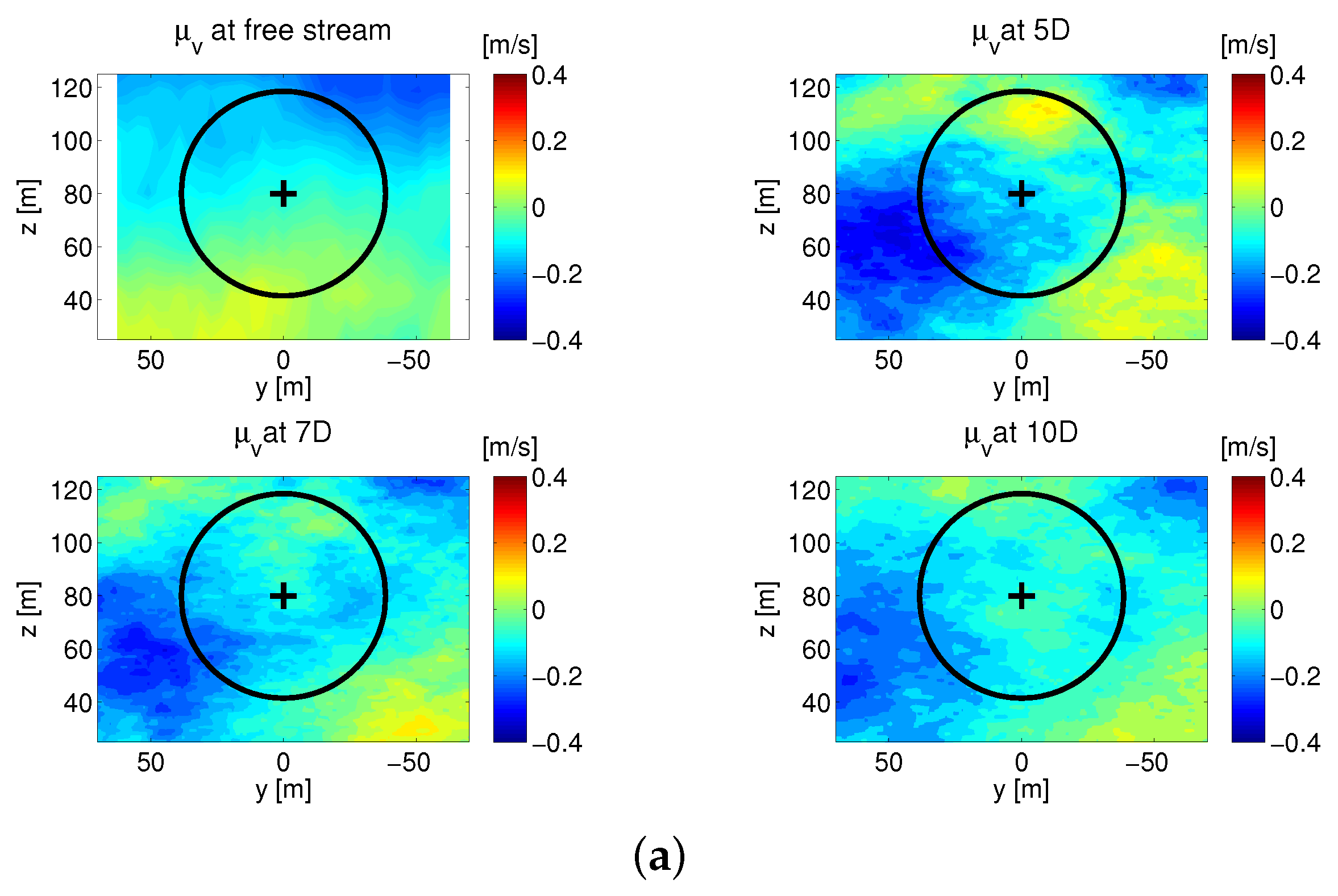
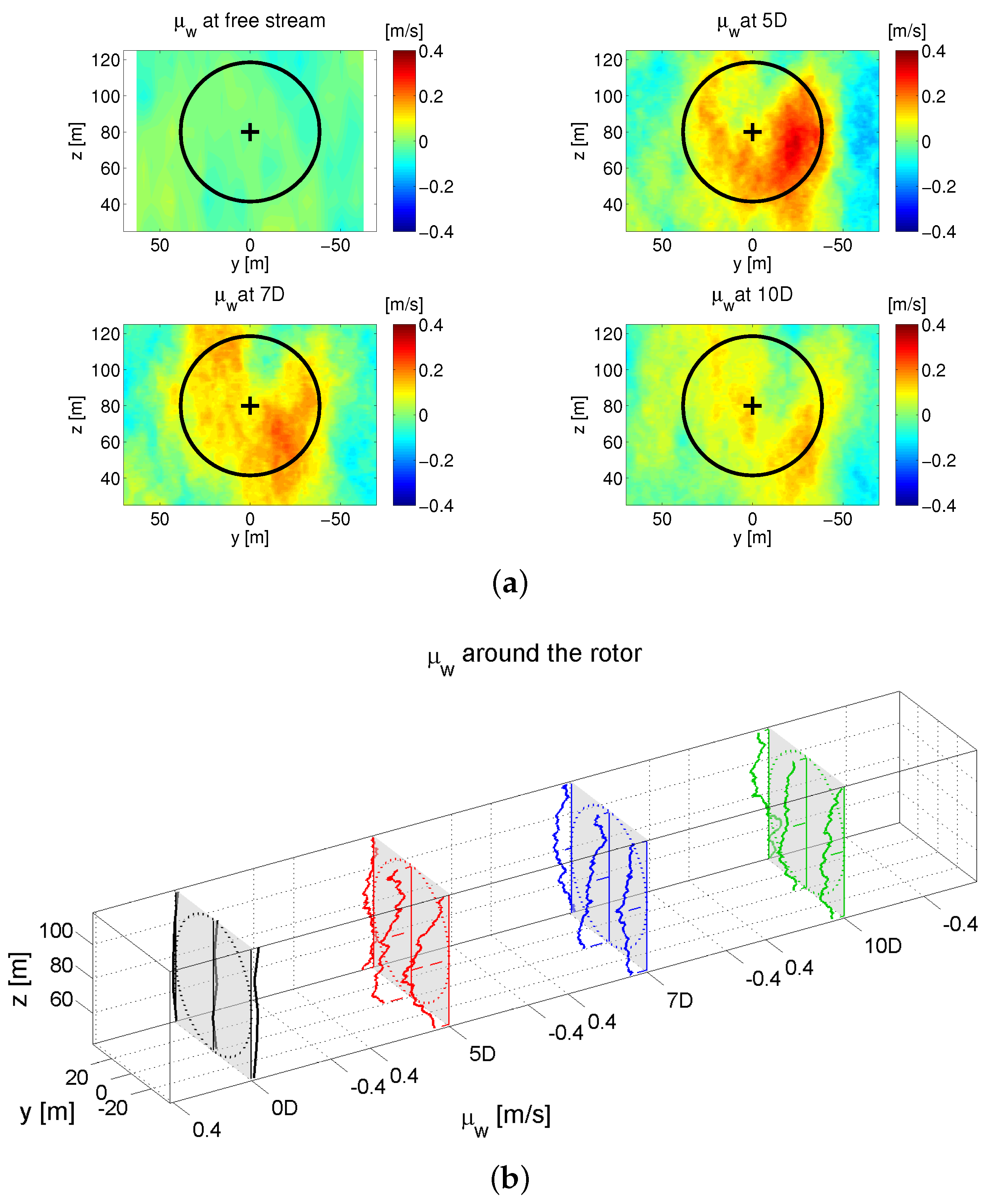
In Figure 9, a vertical motion is shown, due to the rotation of the actuator particularly on the right and toward the lower part of the rotor-swept area. These updrafts are absent in the precursor (free stream). The updraft might be the result of the wake’s meandering behavior [7,23]. In both Figure 8 and Figure 9, the mean wind profiles are not symmetric about the z axis due to the rotation of the wake. Although both the v and w components have small mean values compared to the mean value of the streamwise u component, these asymmetric characteristics need to be embedded in any stochastic wake model that is developed.
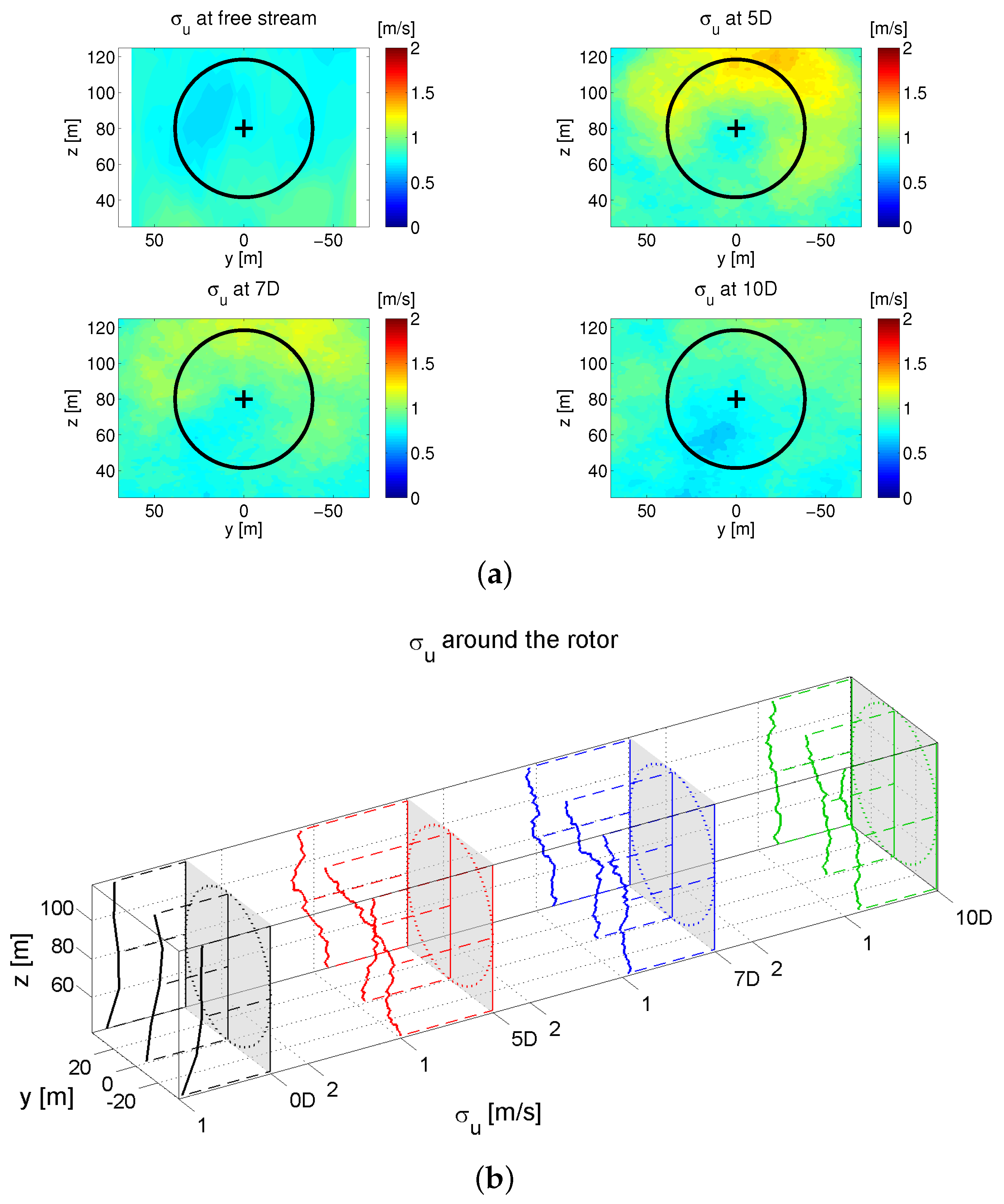
Figure 10 describes the spatial variation of in the free stream and at different downwind locations in the wake. It can be seen that is not uniformly distributed around the rotor. Higher standard deviation levels are seen around the top of the rotor, which were also reported in the study by Troldborg et al. [22]. An asymmetric pattern of the wake field is also evident.
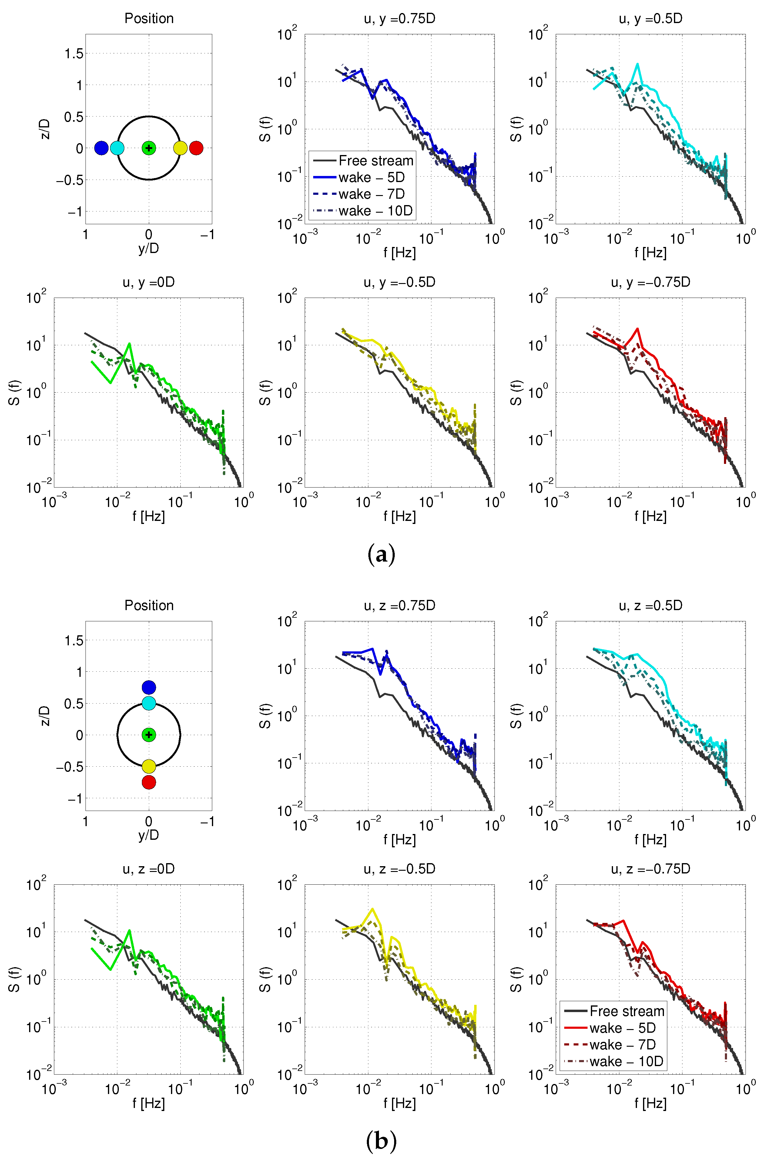
Figure 11 shows power spectral density (PSD) functions for the streamwise u component at different lateral and vertical locations around the rotor hub in the free stream () and in the wake (x = 5D, 7D, and 10D). The thin gray lines indicate the free-stream PSD; the various downstream locations in the wake are indicated by different line patterns. A different color is used for the separate lateral or vertical location for which the PSD function is computed. An increase in overall energy (higher PSD values) is seen around the top, left, and right edges of the rotor. These increases are most evident in a frequency band between 0.02 and 0.20 Hz. The elevated levels at the same locations around the rotor that were seen in Figure 10 may be explained by the increased energy in the PSD functions over a range of frequencies. The decay of these wake-induced increased energy levels as the flow moves downstream is different at the different positions around the rotor; the PSD for the top edge of the rotor shows a slower decay and return to free-stream levels than the PSD at the side edges.
In Figure 8, the precursor (free-stream) lateral wind velocity (v) profile presented in Figure 3 is clearly influenced by wake rotation induced by the torque of the rotor. At the bottom-left of the rotor, the signs of values are different from the precursor profile. This effect is seen to diminish as the flow moves farther downstream. Fluctuations in the vertical profile for the mean v, that develop due to the actuator, also get smaller (i.e., vertical profiles are smoother) as one moves downstream.
Figure 12 shows PSD functions for the v component at different lateral and vertical locations around the rotor rub in the free stream () and in the wake (x = 5D, 7D, and 10D). In this figure, the PSD functions at the left and right sides are seen to be different; at the right side, there is greater energy over frequencies between 0.02 and 0.20 Hz compared to that at the left. This is consistent with the fact that in the wake is not symmetric about the rotor center. The figure shows that PSD functions at the top and bottom of the rotor show different frequency content in the PSD functions.
Figure 13 shows PSD functions for the w component at different lateral and vertical locations around the rotor rub in the free stream () and in the wake (x = 5D, 7D, and 10D). In this figure, increased energy is evident around the top, left, and right edges of the rotor with similar frequency content. In contrast, the PSD for w at the bottom is quite different from the appearance of that for u in Figure 11. The PSD for w at the bottom in the wake shows a relatively slight increase over that of the free stream and shows even a slight decrease at some points. This might be the result of the stream tube expansion: flow passing the actuator interacts with the actuator and is expanded in the lateral and vertical directions. Since the lower boundary is modeled as a wall, the flow between the rotor plane and the lower boundary is vertically compressed. This compression limits the increase of and decreases PSD level.
From the preceding analyses, we note that statistical and spectral characteristics of the waked wind velocity fields show an increase in energy levels compared to those for the free-stream field. Spectral parameters to be developed for a stochastic wake model must account for lateral and vertical asymmetry over the rotor plane. These spatial characteristics must be included in the development of a stochastic model that aims to describe waked wind fields.
4. A Stochastic Wake Model
We discuss the development of an engineering wake model using a stochastic approach that will utilize statistical and spectral information conveyed through the mean and variance fields as well as PSD functions to simulate wake wind fields. Our approach involves application of regression-based procedures to estimate model parameters given the LES-generated waked wind fields. Specifically, multivariate multiple linear regression (MMLR) is used to simultaneously estimate wake stochastic parameters that may then be used in tractable simulation using Fourier techniques. We begin by first estimating free-stream field stochastic parameters (discussed in Section 4.1); then, waked wind field stochastic parameters (discussed in Section 4.2) are estimated by regression in terms of the free-stream parameters and downstream position of interest within the wake. Validation of the stochastic wake model based on MMLR is undertaken in Section 5 where turbine load statistics obtained using the stochastic wake model are compared with those based on the LES-generated waked wind fields.
4.1. Free-Stream Field Stochastic Model Parameters
4.1.1. Regression-Based Free-Stream Mean Field
Using the LES free-stream (precursor) wind fields, we seek to develop a simplified model of the mean wind field (with parameters estimated using regression) as follows:
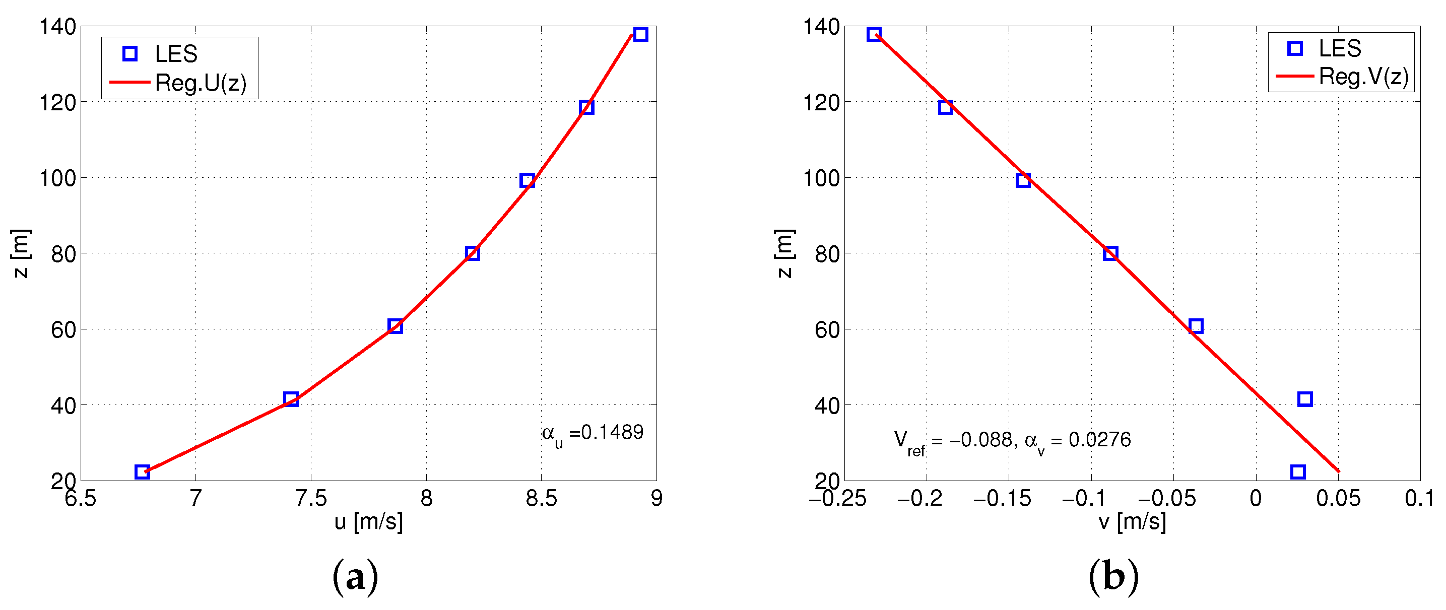
where denotes the free-stream parameters. In addition, is the free-stream mean streamwise wind velocity component variation with height, z, which is modeled using a power-law wind profile; and are reference height and the mean u component wind speed in the free stream at that reference height. In the present study, the reference height is selected as the hub height of the wind turbine considered. Similarly, is the free-stream mean cross-wind velocity component, which is also modeled using a reference wind speed, , but is assumed to vary linearly with z. Finally, is the free-stream mean vertical velocity component which is assumed to be uniform and equal to . With the above model, we can describe mean free-stream wind fields for the three velocity components using five parameters, . Table 1 and Figure 14 summarize results of regression-related estimation of these parameters based on the LES precursor data and an indication of the fit of the mean profiles for u and v using the estimated parameters.
4.1.2. Regression-Based Free-Stream Turbulence Field
To stochastically simulate three-component turbulence time series using an Inverse Fast Fourier Transform (IFFT) approach, we need to define component variances (or standard deviations) and PSD functions. The standard deviation of each component is directly related to its energy level, while PSD functions describe the distribution of energy over all frequencies. We model the vertical variation of the standard deviation for each component in the free stream () using linear functions as follows:
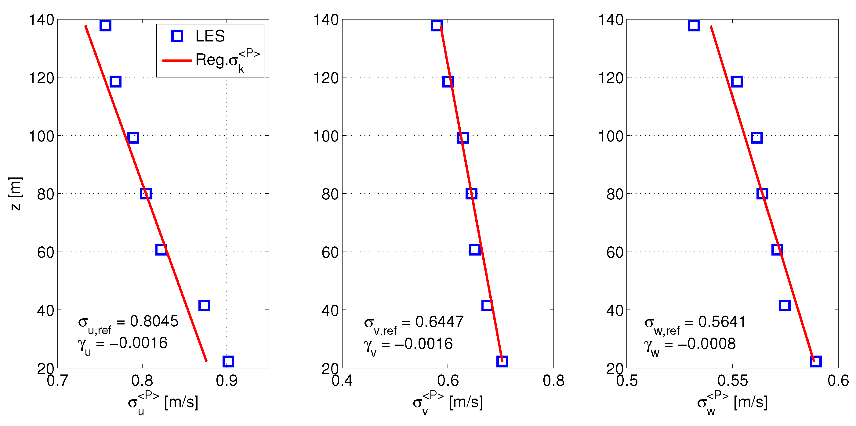
where is the k-component standard deviation at the reference height (which is the selected turbine’s hub height). The selected functional form is similar to that used for . Figure 15 and Table 2 summarize results of regression-related estimation of these parameters based on the LES precursor data and an indication of the fit of the standard deviation profiles for u, v, and w using the estimated parameters.
To model free-stream PSD functions, we use the spectral model proposed by Solari and Piccardo [19], which is defined as follows:
where and are the k-component integral length scale and the roughness length, respectively; In addition, the parameters are constant values, depending on k, that are based on the study by Solari and Piccardo [19]. Note that influences the variation of the PSD function with frequency. As m is assumed, we only need to estimate for each component. Table 3 and Figure 16 summarize results of regression-related estimation of the length scale parameters related to the PSD functions and an indication of the fit of the length scale profiles using the estimated parameters.
With the above model, we can describe the free-stream turbulence wind fields for the three velocity components using nine parameters, . To validate these free-stream models for the turbulence fields, we will discuss a comparison of turbine load statistics based on the time series based on stochastic simulation using the regression-based mean and turbulence field models versus LES-generated free-stream wind fields.
4.2. Wake Field Stochastic Model Parameters
4.2.1. Regression-Based Wake Mean Field
Using the results in Section 4.1.1, we assume the following spatial variation for the wake mean field’s velocity components:
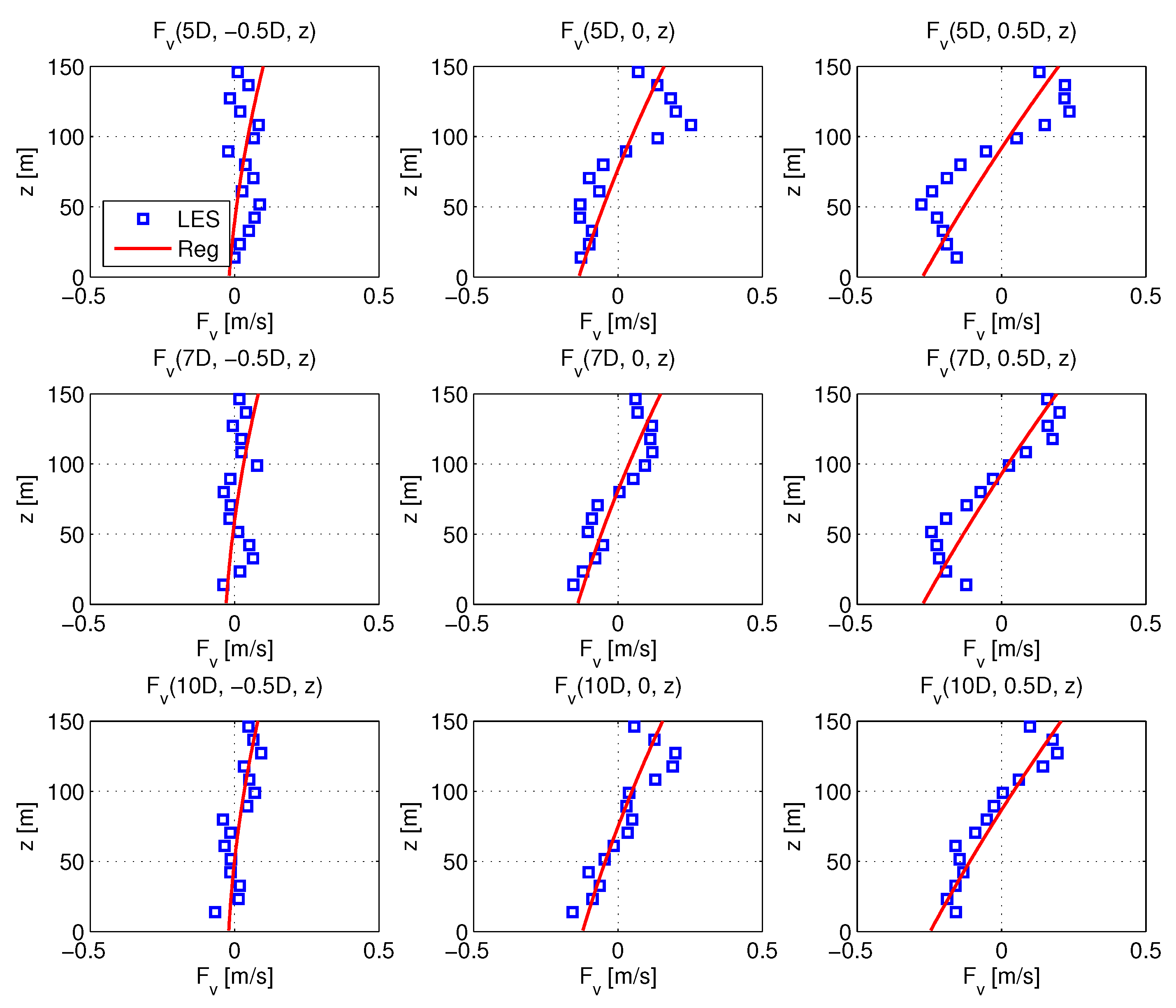
where , , and are, respectively, the u, v, and w component mean wind speeds in the wake. In addition, represents the difference between the free-stream mean and the waked mean for wind velocity component, k. Compared to free-stream mean profiles, the mean profiles for the waked wind fields are modeled to vary, in general, with x, y, and z. Furthermore, , for each component, is formulated as a general quadratic function in x, y, and z. Thus, we have:
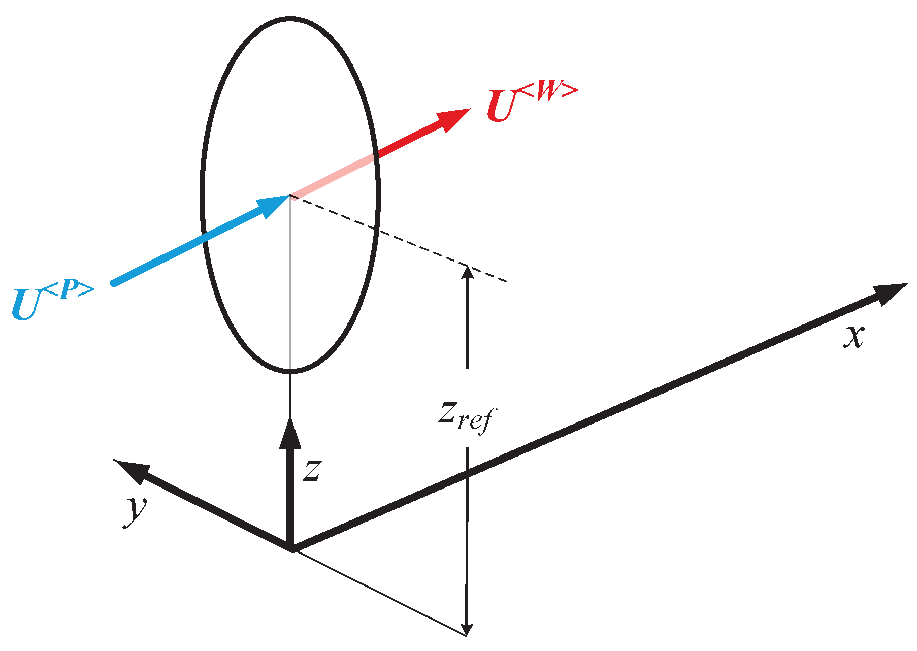
This model, applicable to location , is a quadratic function of this normalized location, , , and . See Figure 17 for a definition of the reference coordinate system where at the wake-generating turbine. In the regression model, we seek to limit collinearity between the predictor variables and to simplify the regression model [24,25]. The parameters, , comprise the vector to be estimated for the mean wake field. If model parameters are independent of each other, simple linear regression may be used to estimate the coefficients involved separately. However, several stochastic parameters collectively help in explaining the physical wake and its influence on the wind field. Thus, the stochastic model parameters are related to each other and MMLR can account for their interaction in a regression setting. Details and applications related to MMLR can be found in the literature [26,27,28,29,30,31].
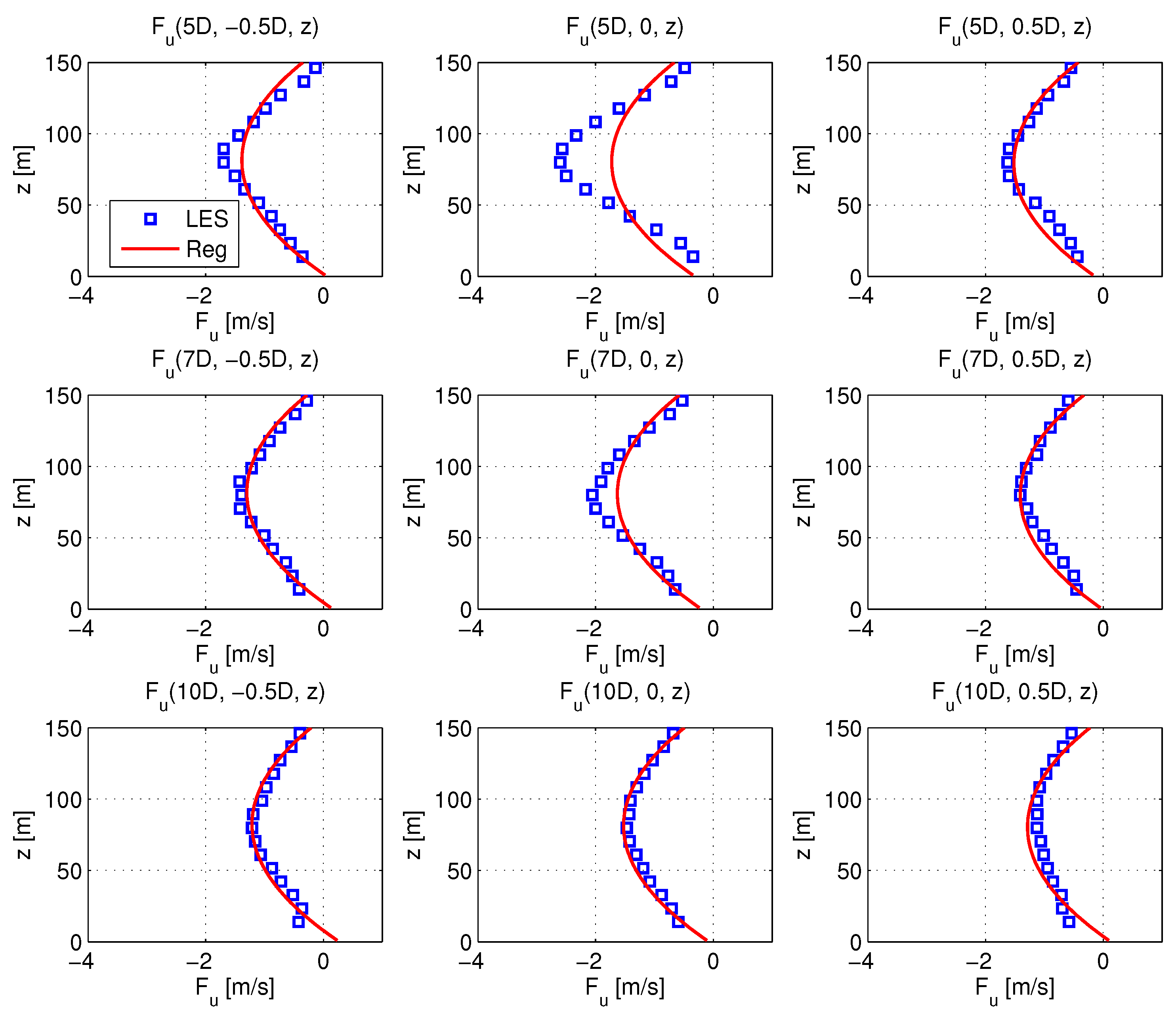
Results of the regression are presented in Table 4 and Table 5. The LES-generated mean wake field is used in the estimation of the regression model parameters. The vertical variation of , , and resulting from the regression are presented in Figure 18, Figure 19 and Figure 20 at downstream locations, , , and .
Although Table 4 suggests that some coefficients are larger than others for each component, because of the relative sizes of the variables with which they form products in the regression model, these larger coefficients are not indicators of importance. The relative importance of each regression term is assessed by estimating associated p values, which are presented in Table 6.
We note that the model fit to the LES data for is not very good and, thus, the coefficient of determination for , in Table 5, is relatively lower than for u and v. Nevertheless, we retain the same simple form for for all the wind velocity components and on studying turbine loads, we can further assess the model validity.
In Figure 18, it is clear that the vertical profiles have a parabolic shape, indicating a wake-related wind speed deficit at hub height. An interesting feature is the differences in the profiles (right of rotor) and (left of rotor), which is in contrast to what is seen in the free-stream mean wind field, , which has lateral symmetry. This suggests that the asymmetric characteristics of the v and w components, due to the rotating actuator line, leads to asymmetry in . The figure shows that vertical and lateral variations represented in the model help describe the trends in . Note that our simple regression model does not adequately capture the spatial characteristics, especially in the near-wake region, e.g., for , where variation in z may be more complex than a quadratic form allows.
Figure 19 indicates that profiles have more lateral asymmetry than ; for instance, shows less vertical variation and influence of the rotating actuator line than does . The characteristics of profile could be related with these results. The counterclockwise-rotating actuator line produces enhanced (positive) lateral wind velocity at the top and a reduced (negative) adjustment at the bottom of rotor, relative to free-stream mean field, . To the right side of the rotor, shows relatively higher gradients than to the left side, which explains the differences between and . Our regression model captures these different vertical gradients between and ; however, the model has some limitations in capturing more complex nonlinearities at .
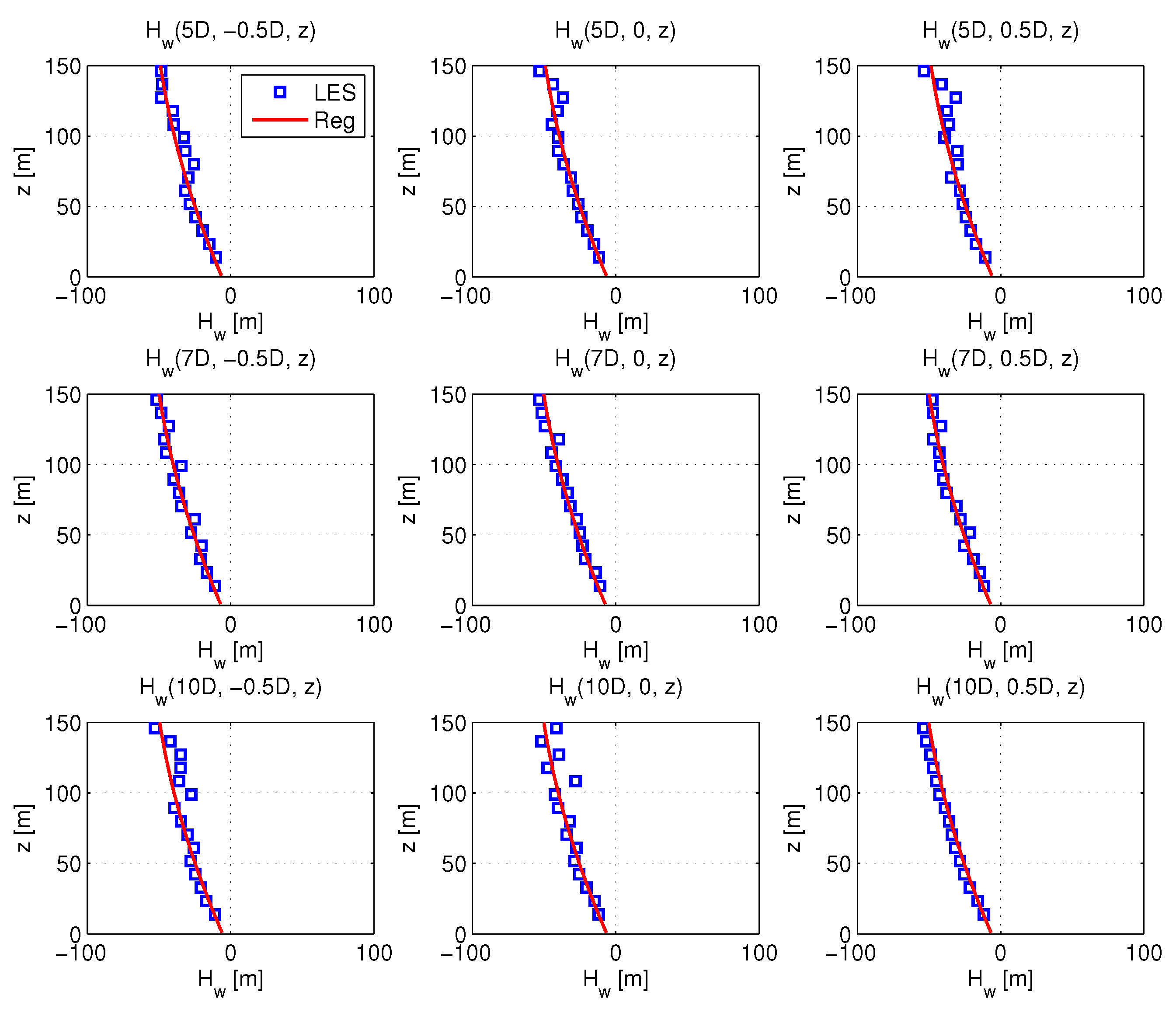
In Figure 20, , as obtained from the LES wake field, shows fairly complex spatial variation vertically, laterally, and as the wake moves downstream. The vertical variation is highly nonlinear; also, laterally, shows greater variation with height than does . Considering the counter-clockwise rotation of the actuator line model, this behavior is understandable. Compared to models for and , the model shows the poorer fits to the LES wake field data (Table 5).
Table 6 presents p-values for each predictor term in the regression. If the p-value for any term exceeds a specified level, changes in that predictor term are not associated with a change in the response. For , -related terms have high p-values, which suggests that these terms cannot adequately describe the decay of with x. An interesting finding is the high p-value for ; due to the parabolic shape for the mean streamwise component, the linear term, , is not so important in the modeling of . Another interesting observation is that the term is associated with a low p-value; this suggests that is explained by a quadratic function, not only in the vertical direction but also in the lateral direction. Compared to , p-values are low for and for ; this suggests that the decay of is well described by including these predictor terms. As is the case for , the -related terms have high p-values in the regression. The term is also associated with high p-values for the regression; this suggests that the lateral asymmetry in is difficult to describe using only a linear term.
4.2.2. Regression-Based Wake Turbulence Field
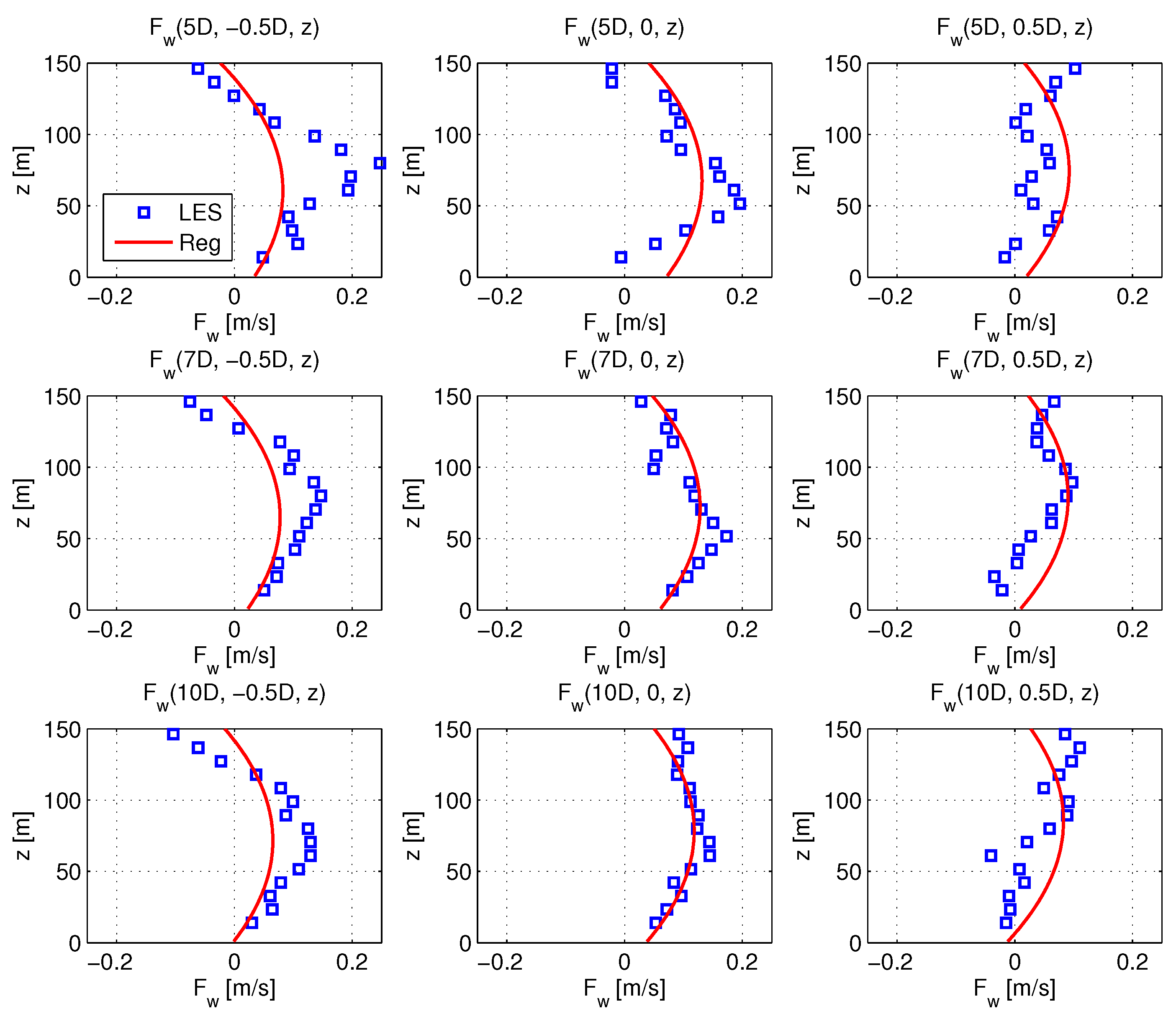
Similar to the regression modeling for the wake mean field, the wake standard deviation variations are modeled as follows:
where is the k component standard deviation in the wake. In addition, is formulated as a general quadratic function in x, y, and z. Thus, we have:
Table 7 and Table 8 as well as Figure 21, Figure 22 and Figure 23 summarize results of the regression studies that use the LES wake wind field data.
In Figure 21, increased values of are seen around the top half of the rotor: there is almost a discontinuity at the hub height evident in the vertical profiles. Additionally, is not symmetric around the centerline (y = 0). This discontinuity and lateral asymmetry arises from the distribution of the free-stream wind field as well as the rotation of actuator lines. These two disparate flow fields introduce different levels of shear/friction around the rotor plane in the wake, which in turn influences the variation of . Our regression model only describe these characteristics very roughly using second-order functions in space. To improve the fit of the model to the LES wake turbulence data, terms such as that allow for discontinuities need to probably be included.
In Figure 22, a sudden increase in is seen around the top half of the rotor. This is likely generated by the wake edge shear, . Over the top half of the rotor, the actuator lines move in the direction while the flow field is in the direction with relatively high speed (see Figure 14b). Over the bottom half of the rotor, the actuator lines move in the direction and the flow field moves with less clearly defined direction and with relatively slower speed. The higher friction in contrasting flow fields occurring over the top half of the rotor result not only in higher values but also in higher values there. As is seen with the vertical profiles, the vertical profiles indicate a changing spatial trend at hub height; the profiles are less sharp than the profiles.
In Figure 23, an increase in is seen around the top half of the rotor. Differences laterally between and are not small. Since the free-stream wind field, , is not significant around the rotor plane and because the actuator lines are rotating counterclockwise, vertical asymmetrical variation in , with higher friction on the right side of the rotor ( area) is understandable. In comparison with the and models, the regression model fits to the LES wake field data appear reasonable or slightly better.
Table 9 presents p-values for each predictor term in the regression. For , the , , and terms have high p-values, indicating that these terms do not aid in the modeling of . In contrast, the and have zero p-values, implying that these terms help with the model predictions. With , it is mainly the , , terms that are associated with low p-values; the other predictive terms are not so significant. Finally, p-values for terms in the regression model show similar trends to that for .
Similar to the PSD functions for the free-steam wind field turbulence components, the wake PSD functions are modeled as follows:
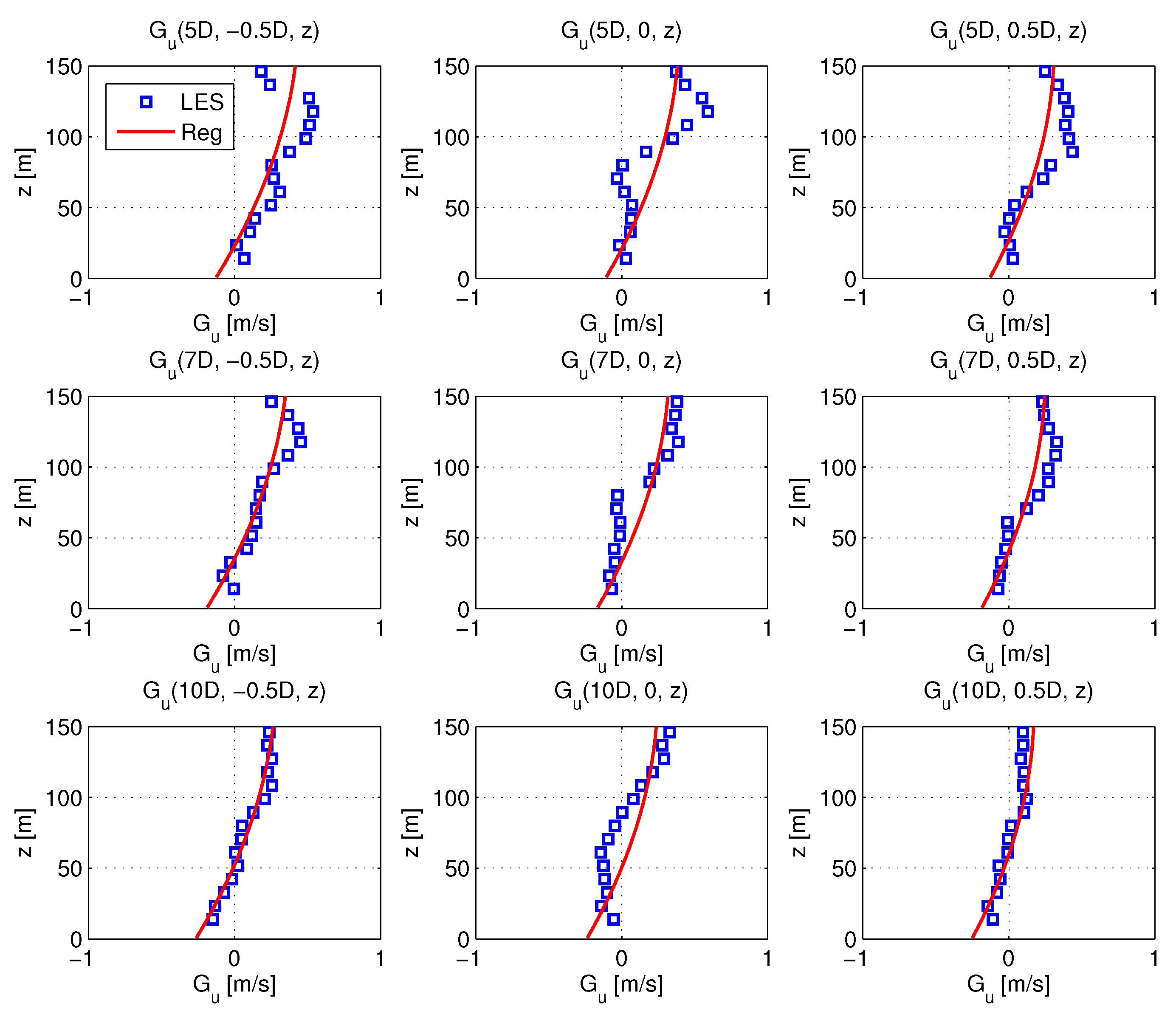
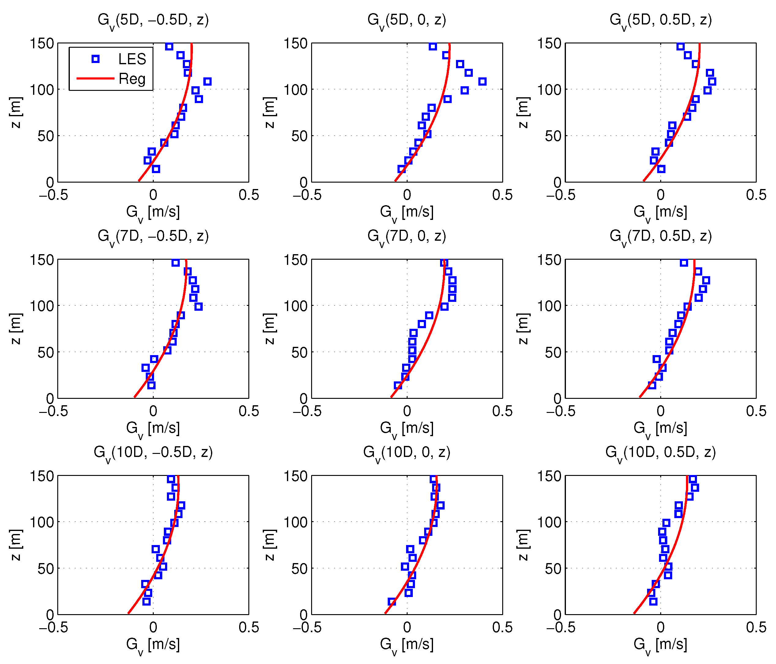
where is the PSD function for turbulence component k in the wake, is the associated integral length scale, and is the difference between and , the free-stream component integral length scale. Note that is estimated from the PSD functions obtained using the LES wake wind field and is formulated in a similar manner to the models for and . The various regression coefficients for the wake field mean and turbulence parameters, , , and , are estimated simultaneously using MMLR. For , we have:
Table 10 and Table 11 as well as Figure 24, Figure 25 and Figure 26 summarize the results of regression for .
In Figure 24, the model predictions indicate considerable variation. Compared to other wake turbulence field parameters, integral length scales are estimated from PSD functions resulting from the LES wake field time series. Limitations on the amount of available data make it difficult to estimate PSD functions; hence, the estimation procedure for has some error which in turn leads to low coefficient of determination values, . Nevertheless, greater changes in the wake streamwise velocity integral length scale, relative to the free stream, are seen around the top half of the rotor. This indicates that the rotation of actuator lines affects not only the turbulence variance of standard deviation (), but also the overall shape of the PSD function. Since the signs of are systematically negative, the integral length scale in the wake, , reduces around the rotor, relative to the free-stream wind field.
In contrast with , Figure 25 indicates smaller variation in the model predictions. Over the top half of the rotor, the values are the most negative; the changes in length scale compared to the free stream are quite similar at different lateral positions relative to the turbine centerline. These length scales also change only slightly as the wake moves downstream. Overall trends in the vertical profiles are adequately described using second-order functions and lead to high values for the regression.
In Figure 26, we see that the general behavior is similar to that found for . Over the top half of the rotor, the values are most negative. Overall trends in the variation are well described using second-order functions and result high values for the regression.
Table 12 presents p-values for each predictor term in the regression. The p-values for the and terms are zero indicating that second-order variation in z describes spatial variation reasonably well. In contrast, p-values for other terms are less significant in predicting length scales.
5. Turbine Response Analysis
To calculate turbine loads, we simulate 20 sets of wind velocity time series based on both the free-stream and the wake models discussed. We employ the Veers method [32] to simulate these wind velocity time series from regressed mean, deviation, and spectral models in Section 4. We assume that space and point coherence functions are the same as in the study by Solari and Piccardo [19]. The length of each time series is 600 s. Wind velocity time series directly from the LES and simulated using an IFFT-based procedure with the stochastic regression models are applied to the WindPACT 1.5-MW wind turbine [33], which has the same size as that of the wake-generating turbine.
Table 13 describes parameters of the model. Turbine loads are calculated using the FAST code [34]. Statistics of turbine loads from the LES and from stochastic simulation using the regression models are compared. In the case of turbine loads from the stochastic simulation, statistics are ensemble-averaged based on 20 simulations. Since waked wind velocity flow fields exhibit lower mean wind speeds and higher standard deviations compared to the free-stream field, it is expected that the dynamics of flow fields might affect the dynamics of the turbine loads. Accordingly, turbine component response maxima, power spectra, and fatigue are also studied.
5.1. Turbine Response with Free-Stream Inflow Velocity Fields
Figure 27 shows power spectra for different turbine loads (IPBM: in-plane bending moment at a blade root; OoPBM: out-of-plane bending moment at a blade root; FATM: fore-aft tower bending moment; SSTM: side-to-side tower bending moment). In both blade bending moment, the highest peak occurs around the 1P frequency (0.26 Hz) because both blade moments are influenced by the turbine’s rotation. In both tower moment power spectra, the highest peak is at the tower’s natural frequency. A second peak is also evident at 3P (0.78 Hz), indicating that the rotor’s rotation does influence loading of the tower. From the figures, it is clear that PSD functions based on the regression models capture characteristics of the LES free stream quite accurately.
Table 14 summarizes standard deviations and maxima for all the turbine loads. Load statistics from the IFFT-based stochastic simulation using the regression model parameters match those based on the LES inflow quite well.
Figure 28 shows 1-Hz equivalent fatigue load (EFL) estimates for the different turbine loads studied. Thin lines on the bars indicate EFL minima and maxima based on 20 simulations. The fatigue loads for the blade moments do not show large variation among the 20 simulations. Tower moments, in contrast, show somewhat greater variability. Overall, averaged values of tower moment fatigue loads from the stochastic simulation are similar to those from the LES-generated free-stream field. All the results involving turbine loads suggest that our stochastic free-stream model matches the LES free-stream wind field acceptably well.
5.2. Turbine Response with Waked Velocity Fields
For the calculation of loads on a turbine in the wake, 20 sets of wind velocity time series are simulated based on the stochastic wake model developed in Section 4.2. Similar to the analyses in Section 5.1, space and point coherence functions are the same as in the study by Solari and Piccardo [19]. Statistics of turbine loads from LES and from the stochastic model are compared and serve to validate the regression-based stochastic wake model. Figure 29 shows power spectra for the different turbine load time series based on only the LES-generated waked wind fields. Compared to the free stream, the frequencies associated with 1P, 2P, and 3P are changed (they are lower at and recover to the free-stream levels farther downstream) and are evident for both blade moments. The mean wind speed deficit in the wake is the main reason for this change since the rotation speed of the blades is related to the mean wind speed. Energy levels at both blade natural frequencies are also changed, though only very slightly. In the case of the tower bending moments, there are some clear differences in load PSDs between the wake and the free stream but these diminish as the wake moves downstream (around ).
Statistics of turbine loads estimated using the stochastic wake model are presented in Table 15. Out-of-plane blade bending moment statistics (standard deviation and maximum) from the stochastic model are very similar to those computed using the LES wind fields. In addition, turbine loads for both the free stream and wake are quite similar; this suggests that the wake does not alter the wind field and turbine loads relative to the free-stream inflow. The mean hub-height velocity of the free-stream wind field in the precursor LES is relatively low (8 m/s) and the mean velocity deficit and standard deviation increase are likely so small as to not significantly influence loads on turbines in the wake.
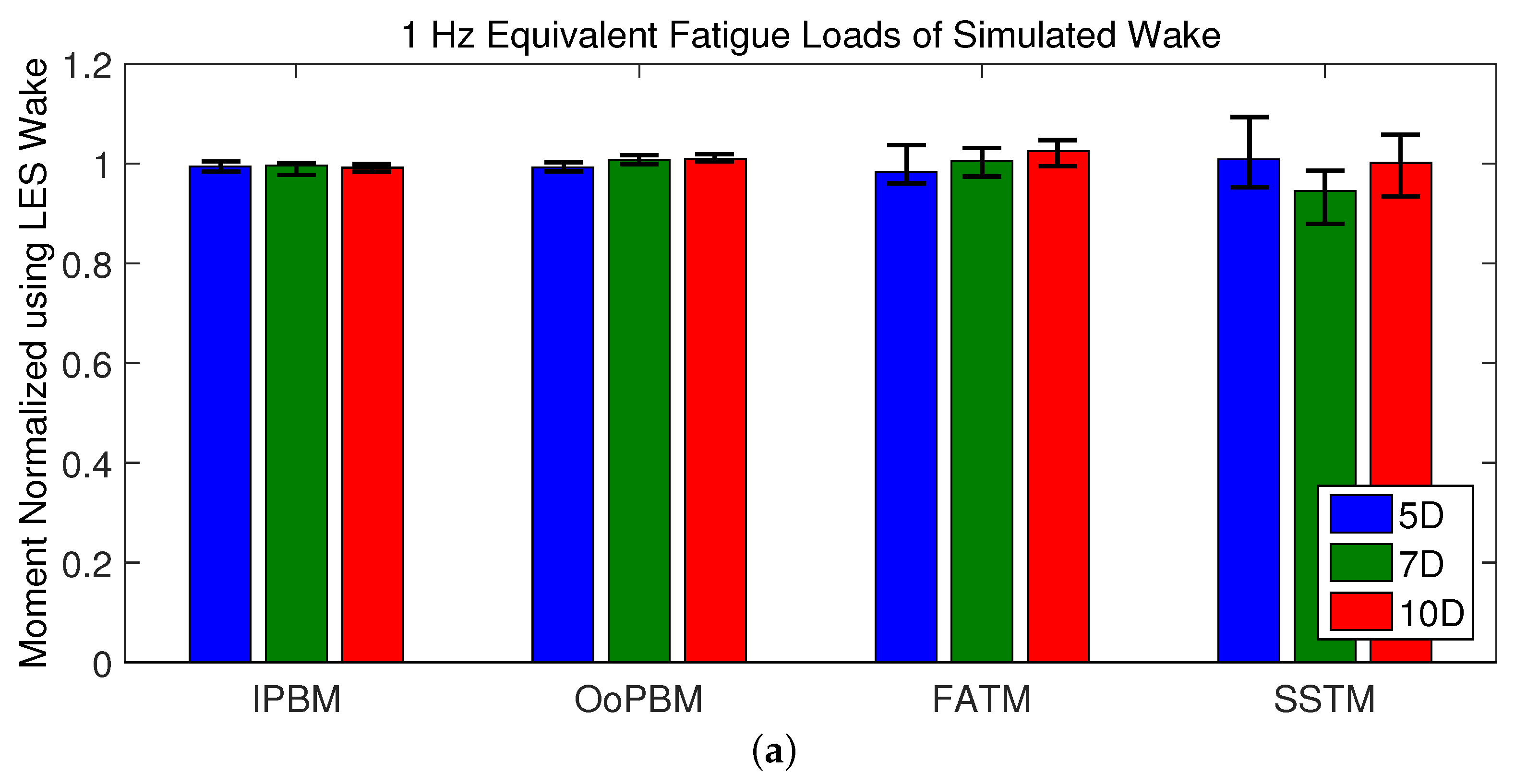
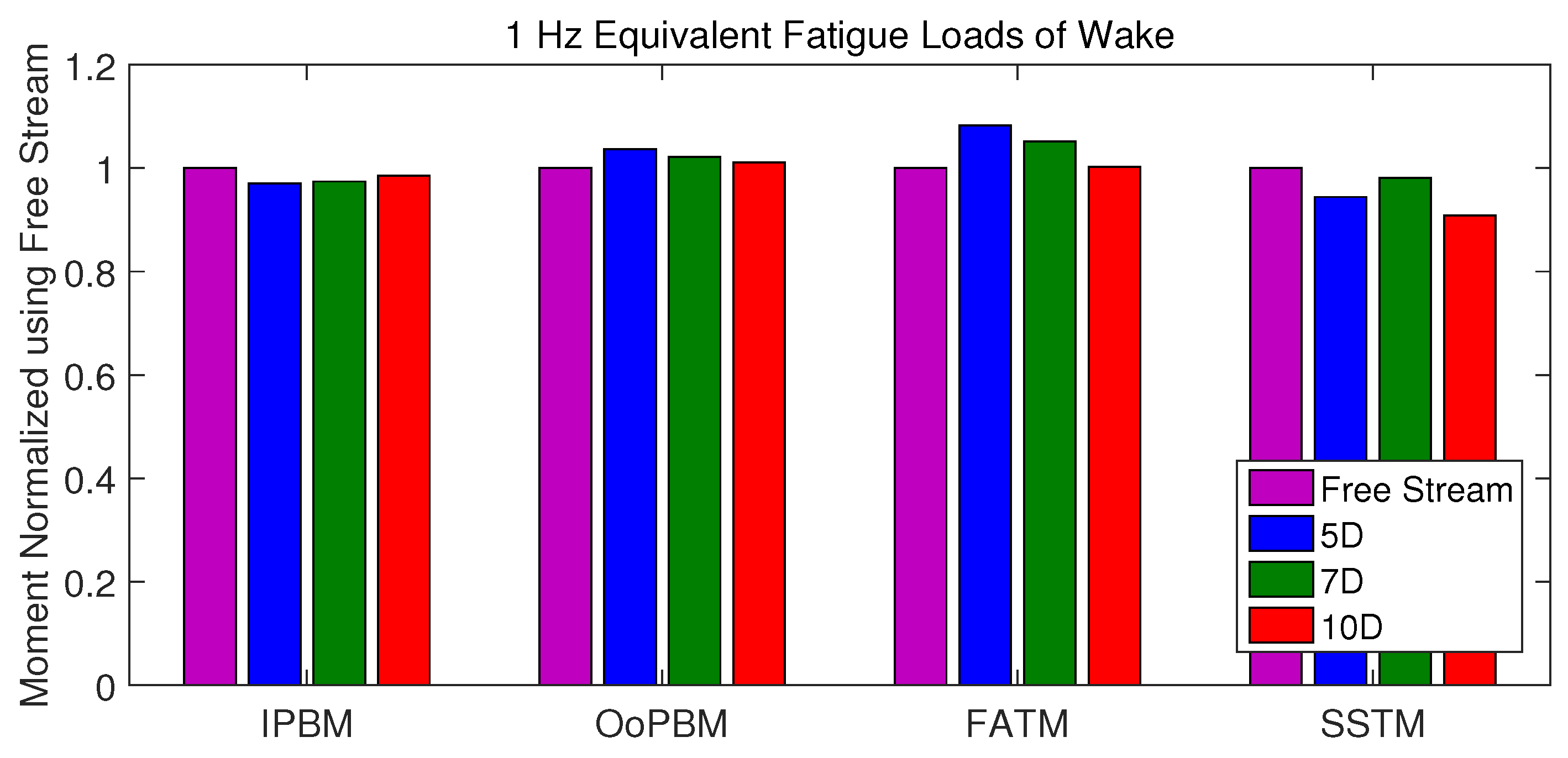
Figure 30 shows normalized 1-Hz EFL estimates for different turbine loads in the free stream and the wake based on use of the stochastic model (the normalization is relative to the LES-generated EFL estimate in each case). The bars present ensemble-averaged values of EFL based on 20 simulations. EFL values in the wake at are slightly higher than at other locations; EFL estimates generally get closer to those from the free stream as the downstream distance increases. This is consistent with the finding in a study by Thomsen and Sørensen [35]. In general, all the normalized EFL estimates are close to unity. This suggests that the stochastic wake model can reproduce the dynamic characteristics of the turbine loads from the LES-generated waked wind fields acceptably well.
Table 16 shows standard deviation and maximum values of the different turbine loads based on stochastic simulation of the wake. For comparison, turbine load statistics based on both LES and Frandsen’s mean and turbulence models [6,36] are included. Generally, similar trends in the load statistics are seen for the stochastic model relative to that for the LES wake fields. This suggests that the regression-based stochastic model captures turbine load statistics reasonably well. Standard deviation and maximum values for the OoPBM and FATM loads from the stochastic model are about 5% higher than those from the LES wake fields. On the other hand, the load statistics for the Frandsen model also show similar trends with those from the LES wake fields.
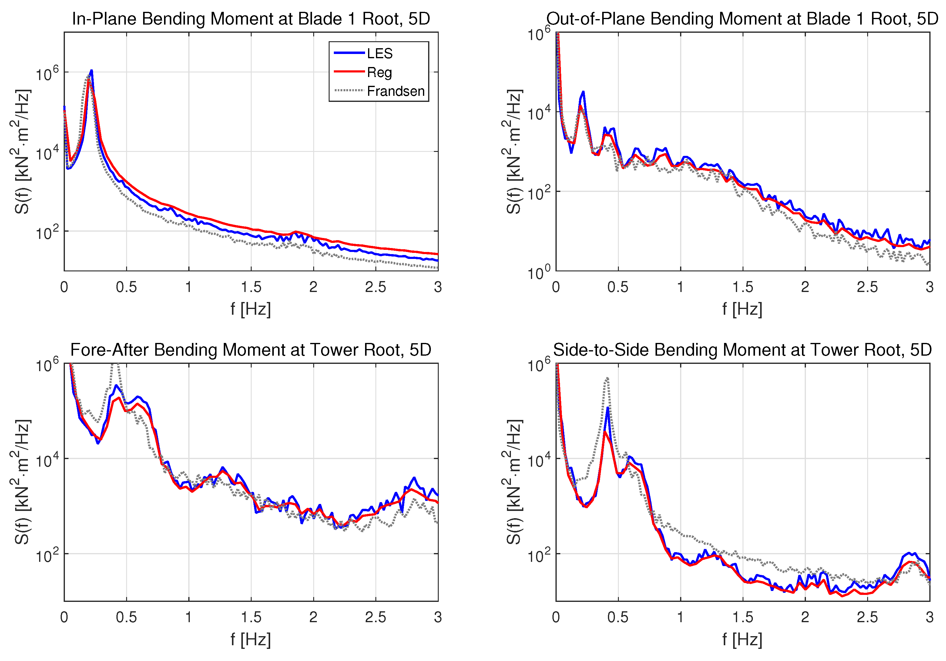
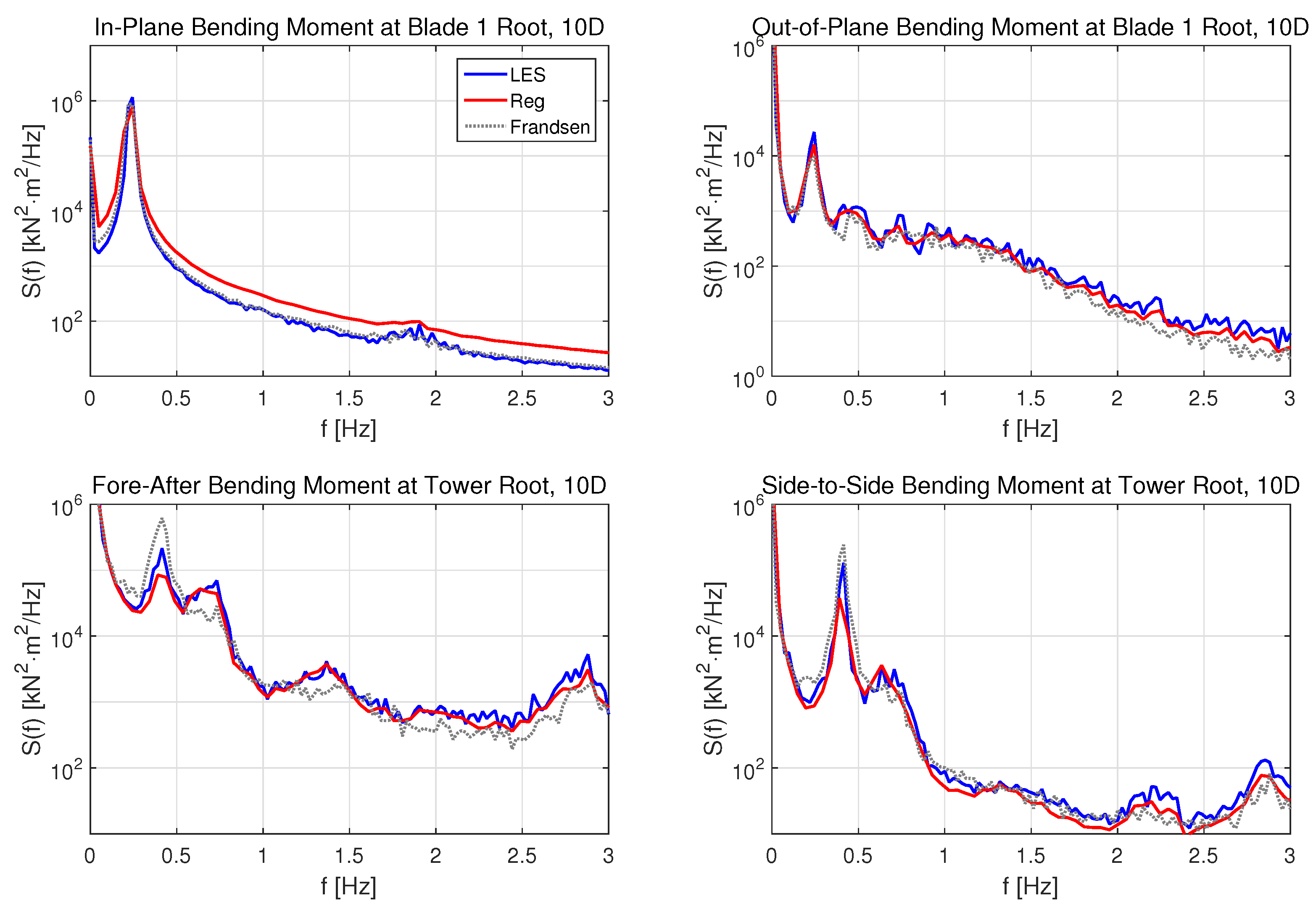
Power spectral density functions of turbine loads based on the stochastic wake model are presented in Figure 31, Figure 32 and Figure 33 for turbines in the wake at , , and , respectively. The turbine load PSD peaks from LES are reasonably well matched with those from the stochastic simulation. Compared to the Frandsen model, the stochastic simulation describes frequency-domain characteristics of the LES waked field better.
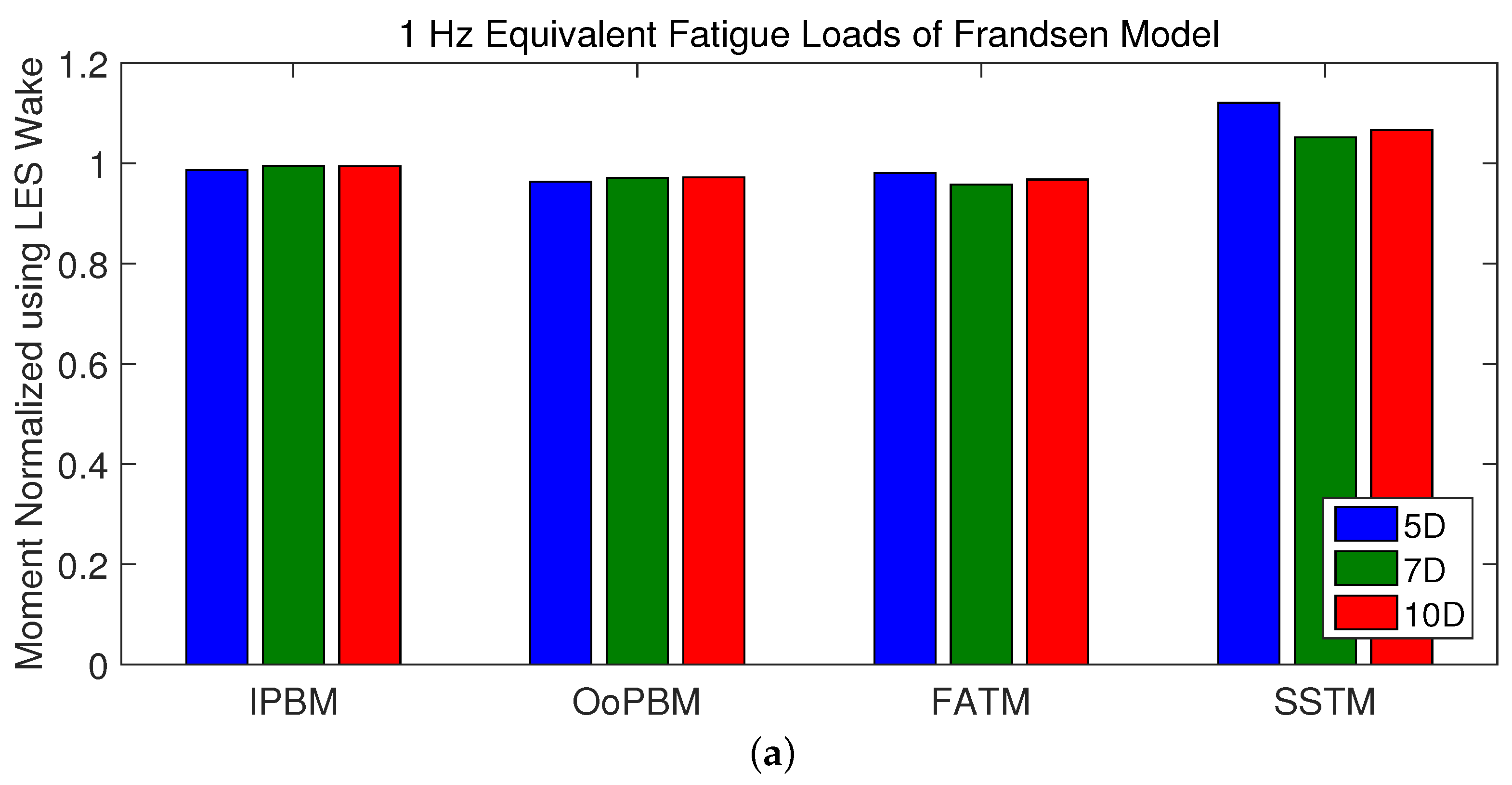
Figure 34 shows normalized 1-Hz EFL estimates for different turbine loads in the wake based on use of both the stochastic model for wake field simulation and the Frandsen model (normalization of the loads is relative to the LES-generated EFL estimate in each case). The bars represent ensemble-averaged values of EFL; the thin horizontal lines at the top indicate minimum and maximum values from 20 simulations. In this figure, all the normalized EFL estimates are close to unity and the variations are quite small. The 1-Hz EFL estimates with the Frandsen model also show a good match for both blade moments and tower moments. These results suggest that the stochastic wake model can reproduce the dynamic characteristics of the turbine loads from the LES-generated waked wind fields acceptably well.
5.3. Summary
We have analyzed stochastic parameters of wind fields downstream of a wake-generating wind turbine. We have developed and demonstrated the use of stochastic wake models using regression. Parameters for the stochastic model were estimated using LES-generated free-stream and waked wind fields. The wake stochastic parameters were related to free-stream stochastic parameters; estimation of the parameters was undertaken using MMLR. The estimation accounted for spatial variation in the mean, standard deviation, and PSD parameters in the wake. Sets of waked wind velocity fields were stochastically simulated using the regression results; these simulated waked wind fields were used in wind turbine load calculations and compared with LES-generated inflow fields and with the Frandsen model. The load analysis results showed that the stochastic wake model yielded wind turbine load statistics, power spectra, and fatigue loads that were comparable to those from LES-generated waked wind fields.
6. Concluding Remarks
This study was focused on the application of stochastic methods for wake modeling. Our interest was in establishing a framework for the stochastic modeling of waked flow fields for wind plants. In particular, we had the following main research objectives: (i) to analyze the dynamic characteristics of waked wind fields using a set of wind velocity time series, downwind of a wake-generating turbine, generated using LES for the estimation of wake stochastic parameters; and (ii) to propose a stochastic approach to simulate waked wind fields over a narrowly defined lateral spatial extent downwind of a wake-generating actuator line.
To generate a set of waked wind velocity time series, a two-step large eddy simulation (LES)—including an atmospheric boundary layer simulation and a waked wind field simulation—was performed. The atmospheric boundary layer with neutral stability conditions was first simulated over a computational domain of 3 km × 3 km × 1 km. A mean wind speed of 8 m/s at 80 m height was the target. Using wind fields from the atmospheric boundary layer simulation, a waked wind field simulation was performed. To simulate the effect of an upwind turbine, an actuator line model of the WindPACT 1.5-MW turbine was operated within the computational domain. From the simulation, a set of waked wind velocity time series at several different locations downwind of the wake-generating turbine was obtained.
We modeled stochastic parameters of the waked wind field using multivariate multiple linear regression (MMLR). The stochastic parameters were evaluated by comparing with associated free-stream field (inflow) parameters. A mean wind deficit and increases in turbulence standard deviation for all three components resulted around the top of the rotor as the free-stream field passed the turbine. Increases in energy of the waked wind field were not uniform at all frequencies. Estimated stochastic wake parameters were modeled with adjustments to free-stream parameters and accounting for location within the wake. To validate the stochastic wake model, a set of stochastically simulated wind velocity fields using IFFT methods were generated and applied in turbine loads simulations. Validation of the model resulted from comparing downstream turbine load statistics based on the stochastic simulation of waked wind fields versus those based directly on the LES wind fields and the wind fields generated using the Frandsen model.
From sets of waked wind fields, the proposed framework is shown to be able to provide a set of stochastic parameters that are associated with the inflow wind field and the wake. A set of wake-associated stochastic model parameters, defined in terms of both inflow wind parameters and turbine parameters, is designed using MMLR. The selected set of wake stochastic parameters is able to generate a set of waked wind velocity time series based on an IFFT approach. Such stochastically generated wind velocity time series capture dynamic characteristics of the wake field data employed reasonably well. Such a stochastic modeling framework could potentially provide waked wind velocity time series without running CFD computations for waked fields since Fourier-based stochastic simulation would require significantly lower computation cost.
This study only demonstrated the framework using a set of LES-generated wake data. The selected stochastic model parameters might not show a good match for wake fields in other inflow conditions because the model parameters developed are estimated from this single set of wake field data. Nevertheless, this framework may be generalized and made more versatile by employing providing multiple sets of wake field data since it is based on a regression scheme. Moreover, this stochastic modeling framework is able to utilize field data, if available. This framework is able to take complex data, experimental or computational, and generate models that are relatively simple and tractable. Ongoing studies are considering application of different wake data with the framework and are focused on improved stochastic parameters for the wake as well as greater spatial downstream coverage.
Acknowledgments
The first two authors gratefully acknowledge the financial support received from the U.S. Department of Energy by way of Subcontract No. AFC-4-42004-01 “Incorporating Wake Effects in Wind Plant Design Criteria” from the National Renewable Energy Laboratory (Prime Contract No. DE-AC36-08GO28308).
Author Contributions
Jae Sang Moon and Lance Manuel conceived of the problem, wrote first drafts of the manuscript, analyzed all the data and developed the stochastic models. Sang Lee and Matthew J. Churchfield defined the large-eddy simulation computational framework and carried out the simulations. Paul Veers contributed with insights, analysis, and additional ideas on presentation.
Conflicts of Interest
The authors declare no conflict of interest.
Abbreviations
The following abbreviations are used in this manuscript:
| EFL | Equivalent fatigue load |
| FATM | Fore-after bending moment at tower base |
| IFFT | Inverse fast fourier transform |
| IPBM | In-plane bending moment at blade root |
| LES | Large Eddy Simulation |
| MMLR | Multivariate Multiple Linear Regression |
| OoPBM | Out-of-plane bending moment at blade root |
| PSD | Power spectral density |
| SSTM | Side-to-side bending moment at tower base |
| D | Turbine diameter |
| Precursor-wake mean wind speed difference model, | |
| Precursor-wake wind speed standard deviation difference model | |
| Precursor-wake integral lengthscale difference model | |
| Precursor k component integral length scale | |
| k component power spectral density from LES | |
| Precursor k component power spectral density profile model | |
| Wake k component power spectral density model | |
| Precursor mean wind speed profile models | |
| Wake mean wind speed profile models | |
| Precursor mean wind speed at reference height | |
| k component, term regression parameter of wake mean wind speed model | |
| k component, term regression parameter of wake wind speed standard deviation model | |
| k component, term regression parameter of wake power spectral density model | |
| f | frequency |
| Longitudinal, lateral, and vertical wind velocity component | |
| Longitudinal, lateral, and vertical position from the tower base | |
| Reference height for precursor profiles model | |
| Gradient of precursor mean wind profile model | |
| Gradient of precursor wind speed standard deviation profile model | |
| k component mean wind speed from LES | |
| k component wind speed standard deviation from LES | |
| Precursor k component wind speed standard deviation profiles model | |
| Wake k component wind speed standard deviation profiles model | |
| Precursor k component wind speed standard deviation at reference height | |
| Precursor k component length scale characterization parameter |
References
- Tran, T.T.; Kim, D.H. A CFD study of coupled aerodynamic-hydrodynamic loads on a semisubmersible floating offshore wind turbine. Wind Energy 2017, 21, 70–85. [Google Scholar] [CrossRef]
- Sánchez Morales, V. Experimental and CFD Analysis of the Flow in the Wake of a Vertical axis Wind Turbine. Ph.D. Dissertation, Universitat Rovira i Virgili, Tarragona, Spain, 2017. [Google Scholar]
- Olivares Espinosa, H. Turbulence Modelling in Wind Turbine Wakes. Ph.D. Thesis, École de Technologie Supérieure, Montréal, QC, Canada, 2017. [Google Scholar]
- Chen, N.; Li, Y.; Xiang, H. A new simulation algorithm of multivariate short-term stochastic wind velocity field based on inverse fast Fourier transform. Eng. Struct. 2014, 80, 251–259. [Google Scholar] [CrossRef]
- Togbenou, K.; Li, Y.; Chen, N.; Liao, H. An efficient simulation method for vertically distributed stochastic wind velocity field based on approximate piecewise wind spectrum. J. Wind Eng. Ind. Aerodyn. 2016, 151, 48–59. [Google Scholar] [CrossRef]
- Frandsen, S. Turbulence and Turbulence-Generated Structural Loading in Wind Turbine Clusters; Technical Report Risø-R-1188; Risø National Laboratory and Technical University of Denmark: Roskilde, Denmark, 2007. [Google Scholar]
- Larsen, G.C.; Madsen, H.A.; Bingol, F.; Mann, J.; Ott, S.; Sørensen, J.N.; Okulov, V.; Troldborg, N.; Nielsen, M.; Thomsen, K.; et al. Dynamic Wake Meandering Modeling; Technical Report Risø-R-1607; Risø National Laboratory and Technical University of Denmark: Roskilde, Denmark, June 2007. [Google Scholar]
- Larsen, T.J.; Larsen, G.C.; Pedersen, M.M.; Enevoldsen, K.; Madsen, H. Validation of the Dynamic Wake Meander model with focus on tower loads. J. Phys. 2017, 854, 012027. [Google Scholar] [CrossRef]
- Larsen, G.C.; Larsen, T.J.; Hansen, K. Loads in wind farms under non-neutral ABL stability conditions—A full-scale validation study of the DWM model. In Proceedings of the International Conference on Future Technologies for Wind Energy WindTech 2017, Boulder CO, USA, 24–26 October 2017. [Google Scholar]
- Sørensen, J.N.; Shen, W.Z. Numerical modeling of wind turbine wakes. J. Fluids Eng. 2002, 124, 393–399. [Google Scholar] [CrossRef]
- Issa, R.I. Solution of the implicitly discretised fluid flow equations by operator-splitting. J. Comput. Phys. 1986, 62, 40–65. [Google Scholar] [CrossRef]
- Gray, D.D.; Giorgini, A. The validity of the Boussinesq approximation for liquids and gases. Int. J. Heat Mass Transf. 1976, 19, 545–551. [Google Scholar] [CrossRef]
- Smagorinsky, J. General circulation experiments with the primitive equations: I. The basic experiment. Mon. Weather Rev. 1963, 91, 99–164. [Google Scholar] [CrossRef]
- Churchfield, M.J.; Lee, S.; Moriarty, P.J.; Martinez, L.A.; Leonardi, S.; Vijayakumar, G.; Brasseur, J.G. A large-eddy simulation of wind-plant aerodynamics. AIAA Paper 2012, 537, 2012. [Google Scholar]
- Churchfield, M.J.; Lee, S.; Michalakes, J.; Moriarty, P.J. A numerical study of the effects of atmospheric and wake turbulence on wind turbine dynamics. J. Turbul. 2012, 13, N14. [Google Scholar] [CrossRef]
- International Electrotechnical Commission. Wind Turbines—Part 1: Design Requirements, IEC-61400-1, Edition 3.0, 2007. IEC 61400-1. Available online: http://www.homepages.ucl.ac.uk/~uceseug/Fluids2/Wind_Turbines/Codes_and_Manuals/BS_EN_61400-1_2005.pdf (accessed on 10 October 2017).
- Sagaut, P. Large Eddy Simulation for Incompressible Flows; Springer: New York, NY, USA, 2002. [Google Scholar]
- Kolmogorov, A. The local structure of turbulence in an incompressible viscous flow for very high reynolds numbers. Dokl. Akad. Nauk SSSR 1941, 30, 301–305. [Google Scholar]
- Solari, G.; Piccardo, G. Probabilistic 3-D turbulence modeling for gust buffeting of structures. Probab. Eng. Mech. 2001, 16, 73–86. [Google Scholar] [CrossRef]
- Kaimal, J.C.; Wyngaard, J.C.; Izumi, Y.; Coté, O.R. Spectral characteristics of surface-layer turbulence. Q. J. R. Meteorol. Soc. 1972, 98, 563–589. [Google Scholar] [CrossRef]
- Von Kármán, T. Progress in the statistical theory of turbulence. Proc. Natl. Acad. Sci. USA 1948, 34, 530. [Google Scholar] [CrossRef] [PubMed]
- Troldborg, N. Actuator Line Modeling of Wind Turbine Wakes. Ph.D. Thesis, Danish Technical University, Lyngby, Denmark, 2008. [Google Scholar]
- Espana, G.; Aubrun, S.; Loyer, S.; Devinant, P. Spatial study of the wake meandering using modelled wind turbines in a wind tunnel. Wind Energy 2011, 14, 923–937. [Google Scholar] [CrossRef]
- Stewart, G.W. Collinearity and least squares regression. Stat. Sci. 1987, 2, 68–84. [Google Scholar] [CrossRef]
- Belsley, D.A.; Kuh, E.; Welsch, R.E. Regression Diagnostics: Identifying Influential Data and Sources of Collinearity; John Wiley & Sons: New York, NY, USA, 2005; Volume 571. [Google Scholar]
- Hair, J.; Knapp, G. Multivariate Multiple Regression; Wiley StatsRef: Statistics Reference Online; John Wiley & Sons, Ltd.: Hoboken, NJ, USA, 2014. [Google Scholar]
- Hair, J.F.; Black, W.C.; Babin, B.J.; Anderson, R.E.; Tatham, R.L. Multivariate Data Analysis; Pearson Prentice Hall: Upper Saddle River, NJ, USA, 2006; Volume 6. [Google Scholar]
- Breiman, L.; Friedman, J.H. Predicting Multivariate Responses in Multiple Linear Regression. J. R. Stat. Soc. B 1997, 59, 3–54. [Google Scholar] [CrossRef]
- Clack, C.T. Modeling solar irradiance and solar PV power output to create a resource assessment using linear multiple multivariate regression. J. Appl. Meteorol. Climatol. 2017, 56, 109–125. [Google Scholar] [CrossRef]
- Valente, G.; Castellanos, A.L.; Vanacore, G.; Formisano, E. Multivariate linear regression of high-dimensional fMRI data with multiple target variables. Hum. Brain Mapp. 2014, 35, 2163–2177. [Google Scholar] [CrossRef] [PubMed]
- Malinverni, S.; Gennotte, A.F.; Schuster, M.; De Wit, S.; Mols, P.; Libois, A. Adherence to HIV post exposure prophylaxis: A multivariate regression analysis of a 5 years prospective cohort. J. Infect. 2017. [Google Scholar] [CrossRef] [PubMed]
- Veers, P. Three-Dimensional Wind Simulation; Technical Report SAND88-0152; Sandia National Laboratory: Albuquerque NM, USA, 1988. [Google Scholar]
- Malcolm, D.J.; Hansen, A.C. WindPACT Turbine Rotor Design Study: June 2000–June 2002 (Revised); No. NREL/SR-500-32495; National Renewable Energy Laboratory (NREL): Golden, CO, USA, 2006.
- Jonkman, J.M.; Buhl, M.L., Jr. FAST User’s Guide; Technical Report NREL/EL-500-38230; National Renewable Energy Laboratory: Golden, CO, USA, 2005.
- Thomsen, K.; Sørensen, P. Fatigue loads for wind turbines operating in wakes. J. Wind Eng. Ind. Aerodyn. 1999, 80, 121–136. [Google Scholar] [CrossRef]
- Frandsen, S.; Barthelmie, R.; Pryor, S.; Rathmann, O.; Larsen, S.; Højstrup, J.; Thøgersen, M. Analytical modelling of wind speed deficit in large offshore wind farms. Wind Energy 2006, 9, 39–53. [Google Scholar] [CrossRef]
Figure 1.
Dimensions of the computational domain.
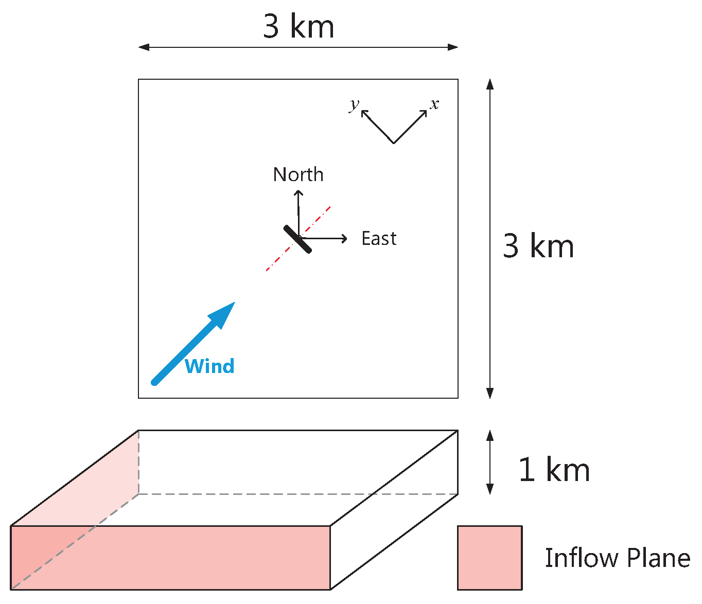
Figure 2.
A horizontal plane through the free-stream wind velocity field near the ground ( m).

Figure 3.
Variation in a vertical plane of the free-stream wind velocity mean and standard deviation.
Figure 3.
Variation in a vertical plane of the free-stream wind velocity mean and standard deviation.
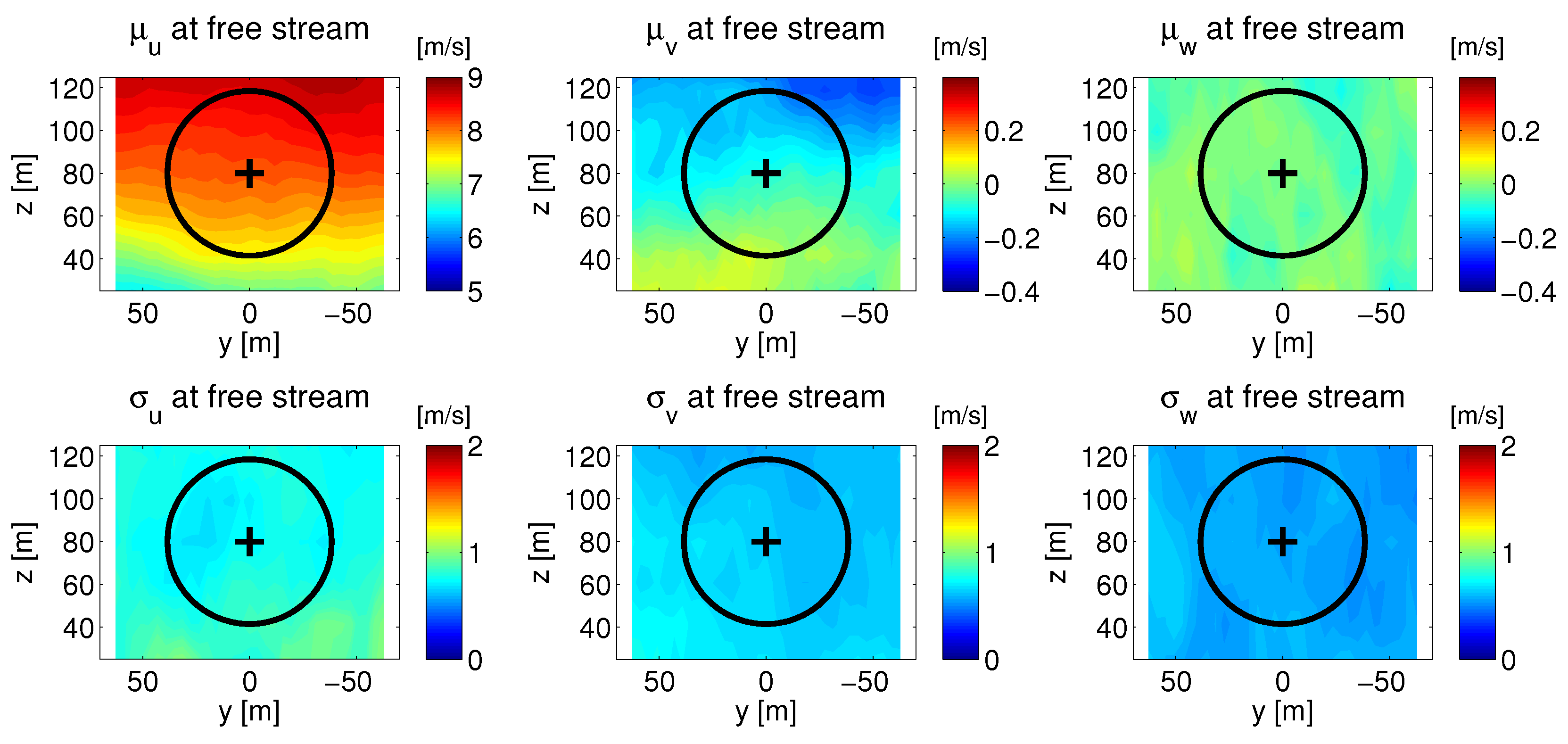
Figure 4.
Power spectra for the three free-stream turbulence components at different heights.

Figure 5.
Power spectra for the three free-stream turbulence components; different locations.
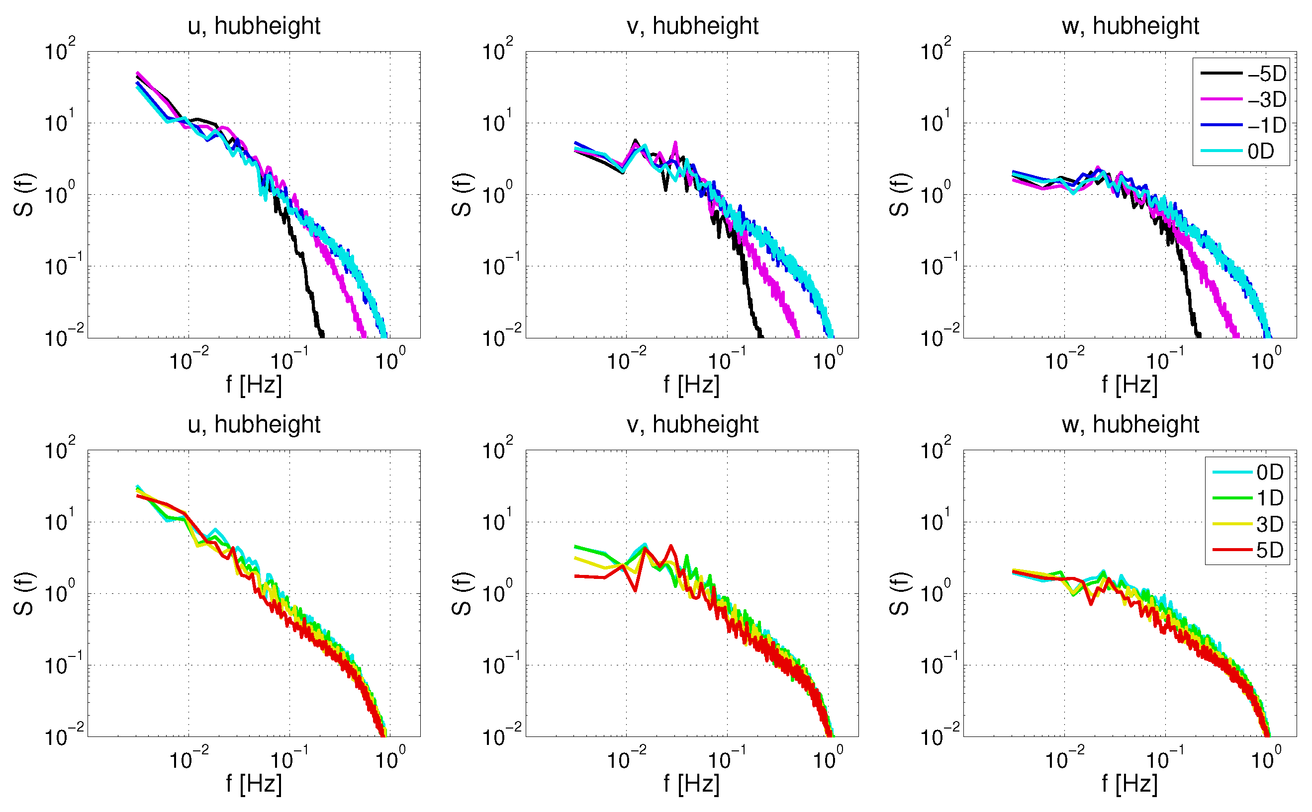
Figure 6.
Coherence functions for the three free-stream turbulence components with the same lateral separation (19.25 m) at different elevations.
Figure 6.
Coherence functions for the three free-stream turbulence components with the same lateral separation (19.25 m) at different elevations.
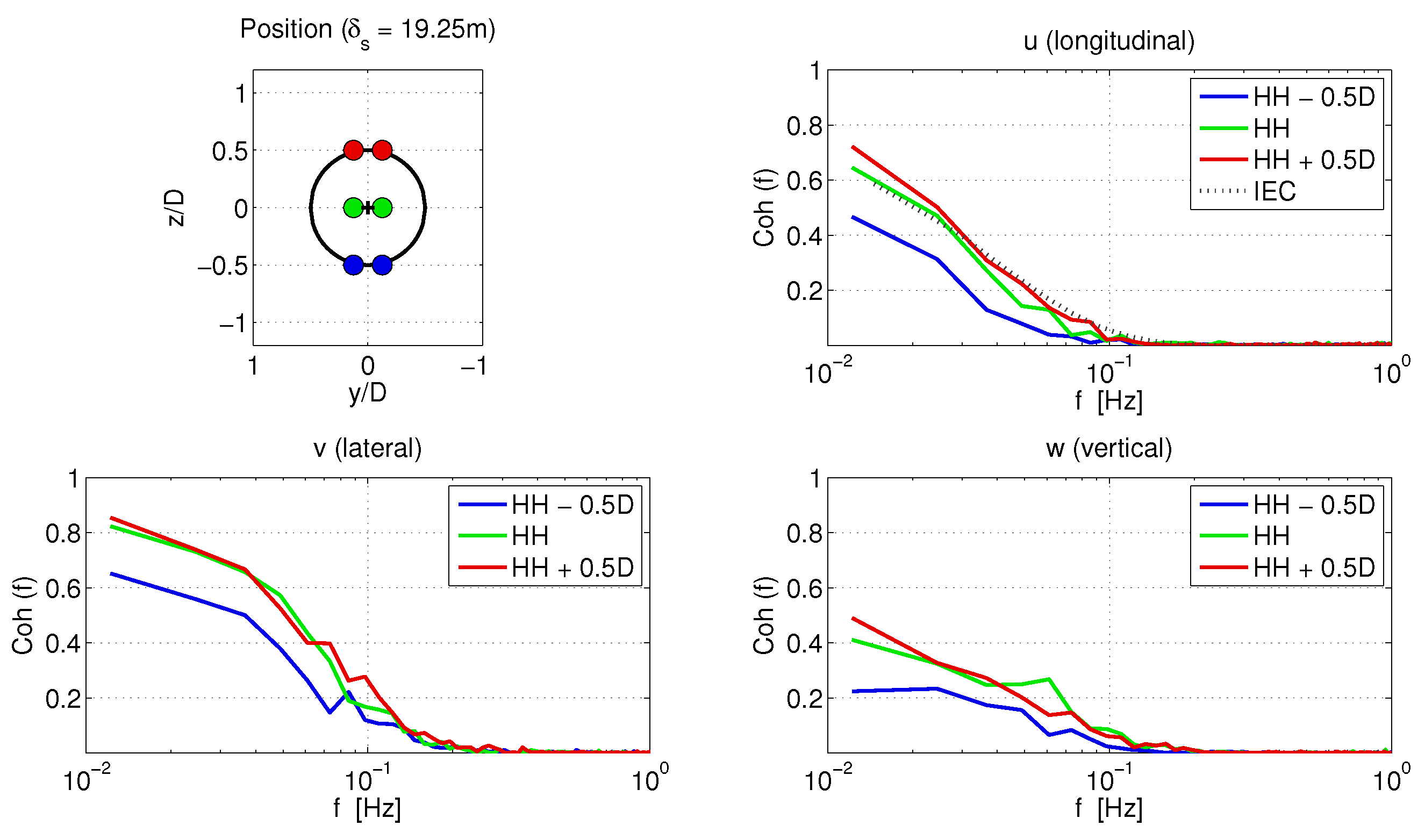
Figure 7.
Spatial variation in the waked field versus the free-stream field: (a) variation of in vertical planes; and (b) profile of .
Figure 7.
Spatial variation in the waked field versus the free-stream field: (a) variation of in vertical planes; and (b) profile of .
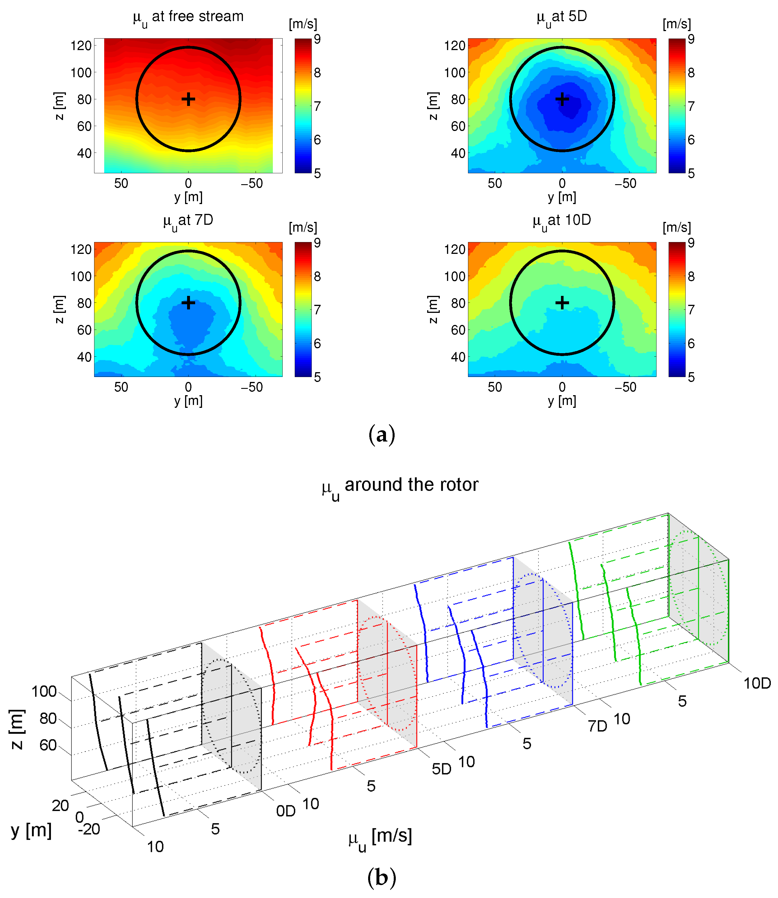
Figure 8.
Spatial variation in the waked field versus the free-stream field: (a) variation of in vertical planes; and (b) profile of .
Figure 8.
Spatial variation in the waked field versus the free-stream field: (a) variation of in vertical planes; and (b) profile of .

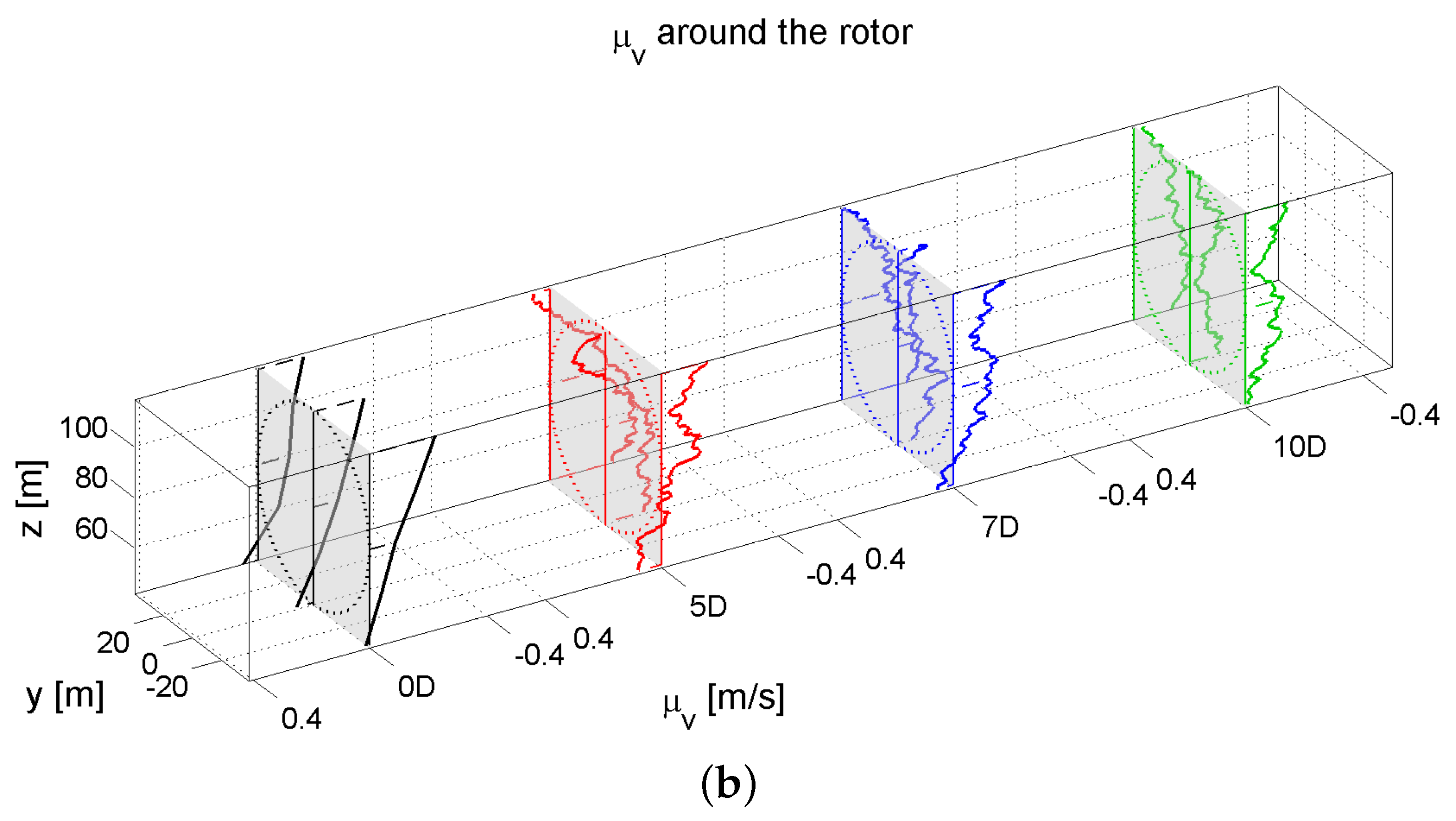
Figure 9.
Spatial variation in the waked field versus the free-stream field: (a) variation of in vertical planes; and (b) profile of .
Figure 9.
Spatial variation in the waked field versus the free-stream field: (a) variation of in vertical planes; and (b) profile of .

Figure 10.
Spatial variation in the waked field versus the free-stream field: (a) variation of in vertical planes; and (b) profile of .
Figure 10.
Spatial variation in the waked field versus the free-stream field: (a) variation of in vertical planes; and (b) profile of .

Figure 11.
Power spectral density functions of u at , 5D, 7D, and 10D: (a) lateral variation; and (b) vertical variation.
Figure 11.
Power spectral density functions of u at , 5D, 7D, and 10D: (a) lateral variation; and (b) vertical variation.

Figure 12.
Power spectral density functions of v at , 5D, 7D, and 10D: (a) lateral variation; and (b) vertical variation.
Figure 12.
Power spectral density functions of v at , 5D, 7D, and 10D: (a) lateral variation; and (b) vertical variation.
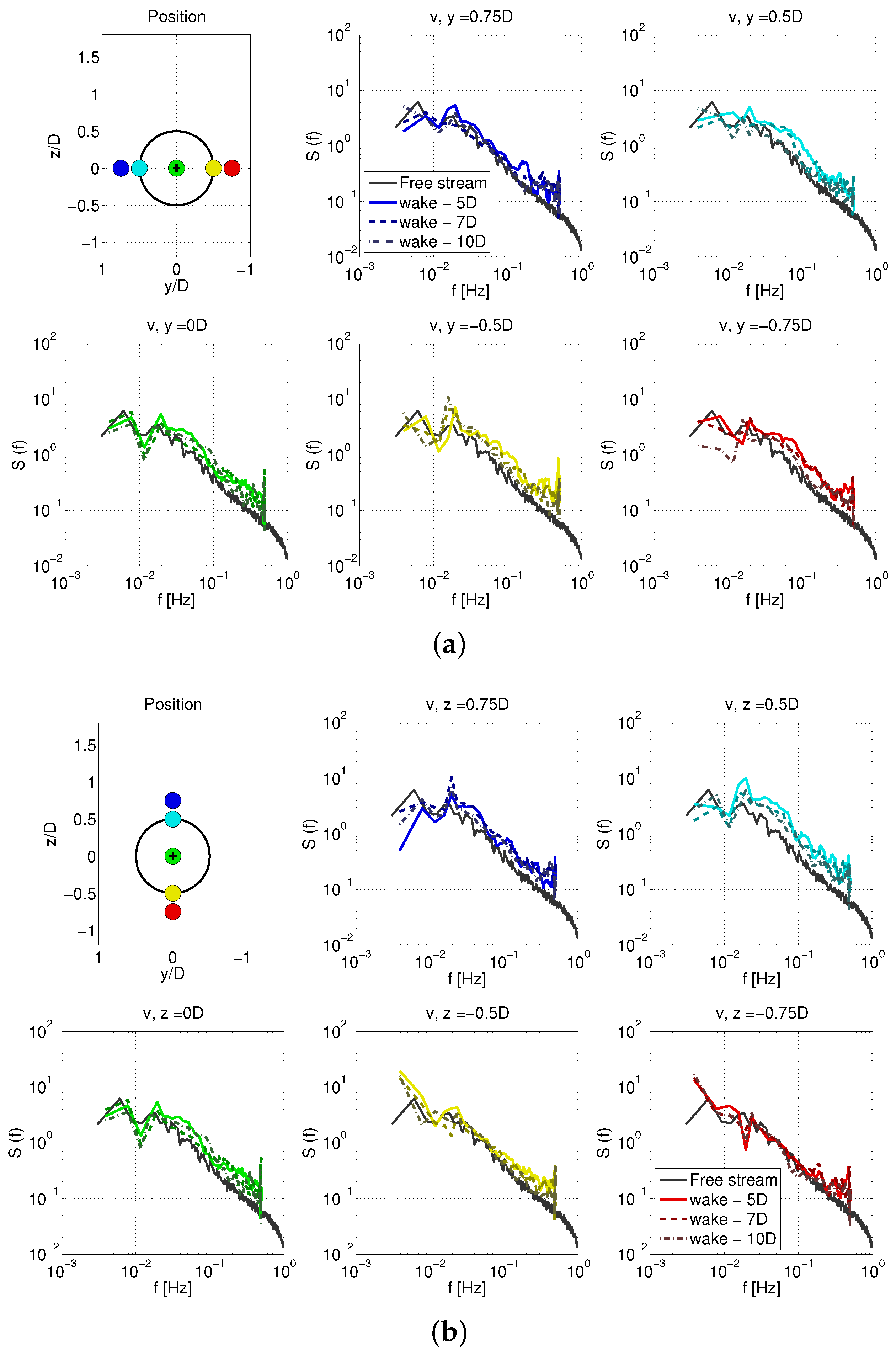
Figure 13.
Power spectral density functions of w at , 5D, 7D, and 10D: (a) lateral variation; and (b) vertical variation.
Figure 13.
Power spectral density functions of w at , 5D, 7D, and 10D: (a) lateral variation; and (b) vertical variation.
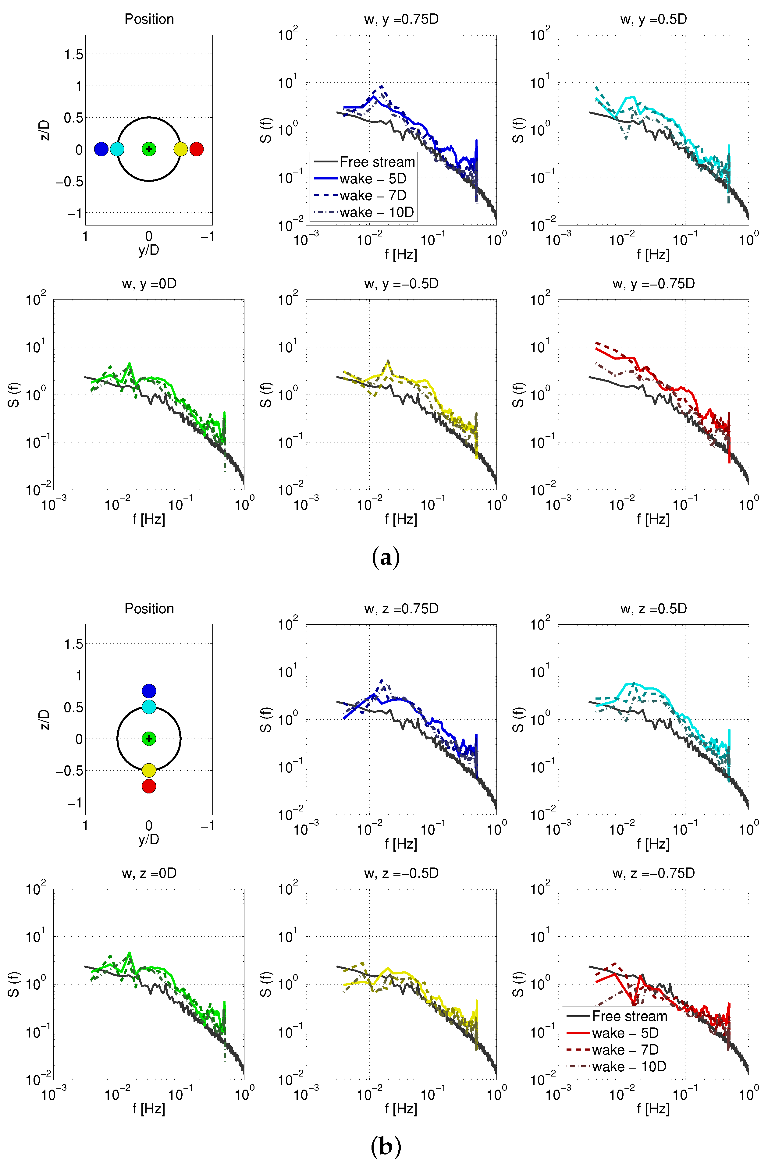
Figure 14.
Free-stream mean profiles: regression vs. Large-Eddy Simulation (LES) data: (a) free-stream u component mean profile; and (b) free-stream v component mean profile.
Figure 14.
Free-stream mean profiles: regression vs. Large-Eddy Simulation (LES) data: (a) free-stream u component mean profile; and (b) free-stream v component mean profile.

Figure 15.
Free-stream standard deviation profiles: regression vs. LES data.

Figure 16.
Free-stream PSD length scale profiles: regression vs. LES data.
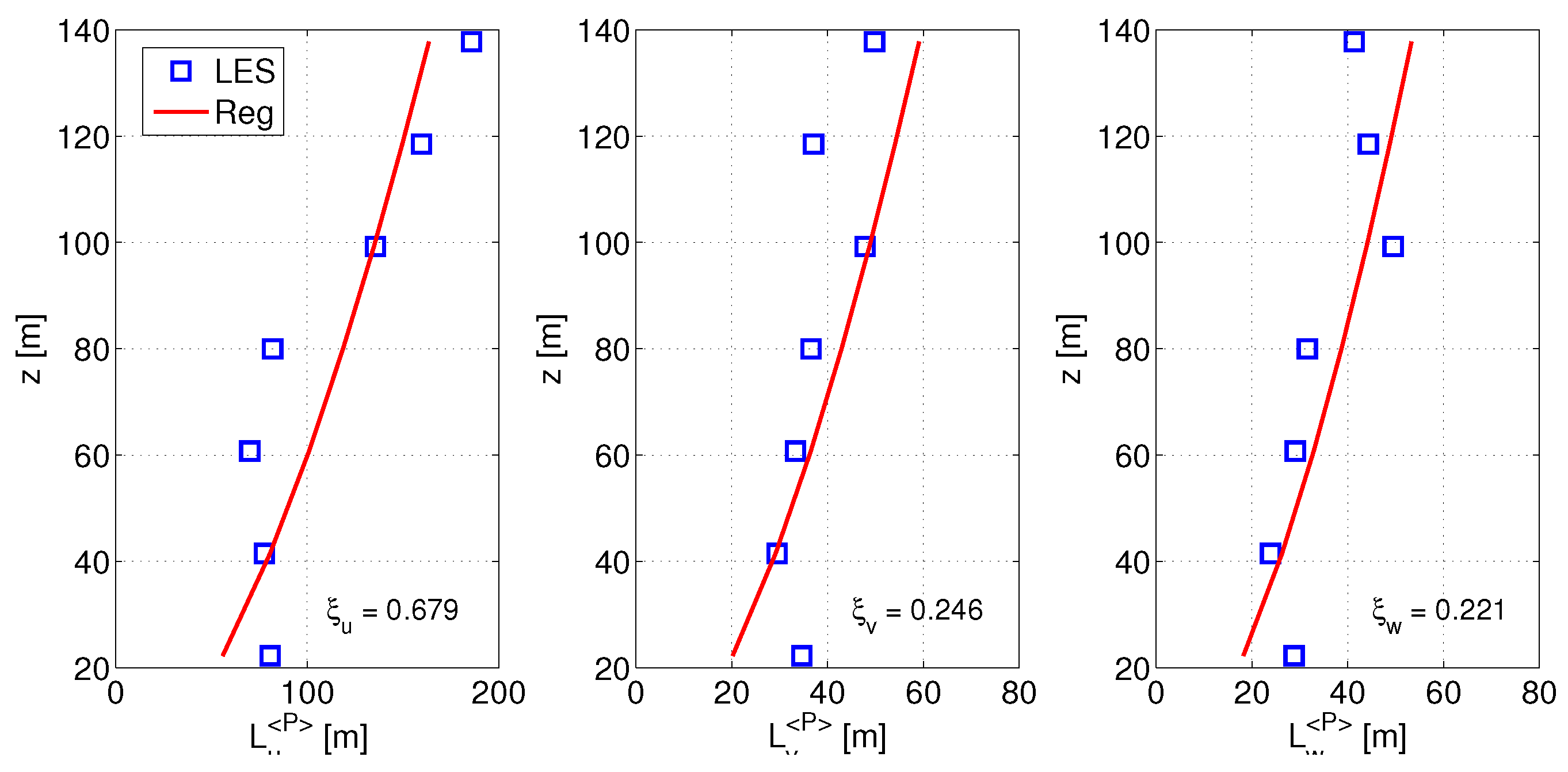
Figure 17.
Coordinate system definition for reference.

Figure 18.
Spatial variation of : LES versus regression-based estimation.

Figure 19.
Spatial variation of : LES versus regression-based estimation.

Figure 20.
Spatial variation of : LES versus regression-based estimation.

Figure 21.
Spatial variation of : LES versus regression-based estimation.

Figure 22.
Spatial variation of : LES versus regression-based estimation.

Figure 23.
Spatial variation of : LES versus regression-based estimation.
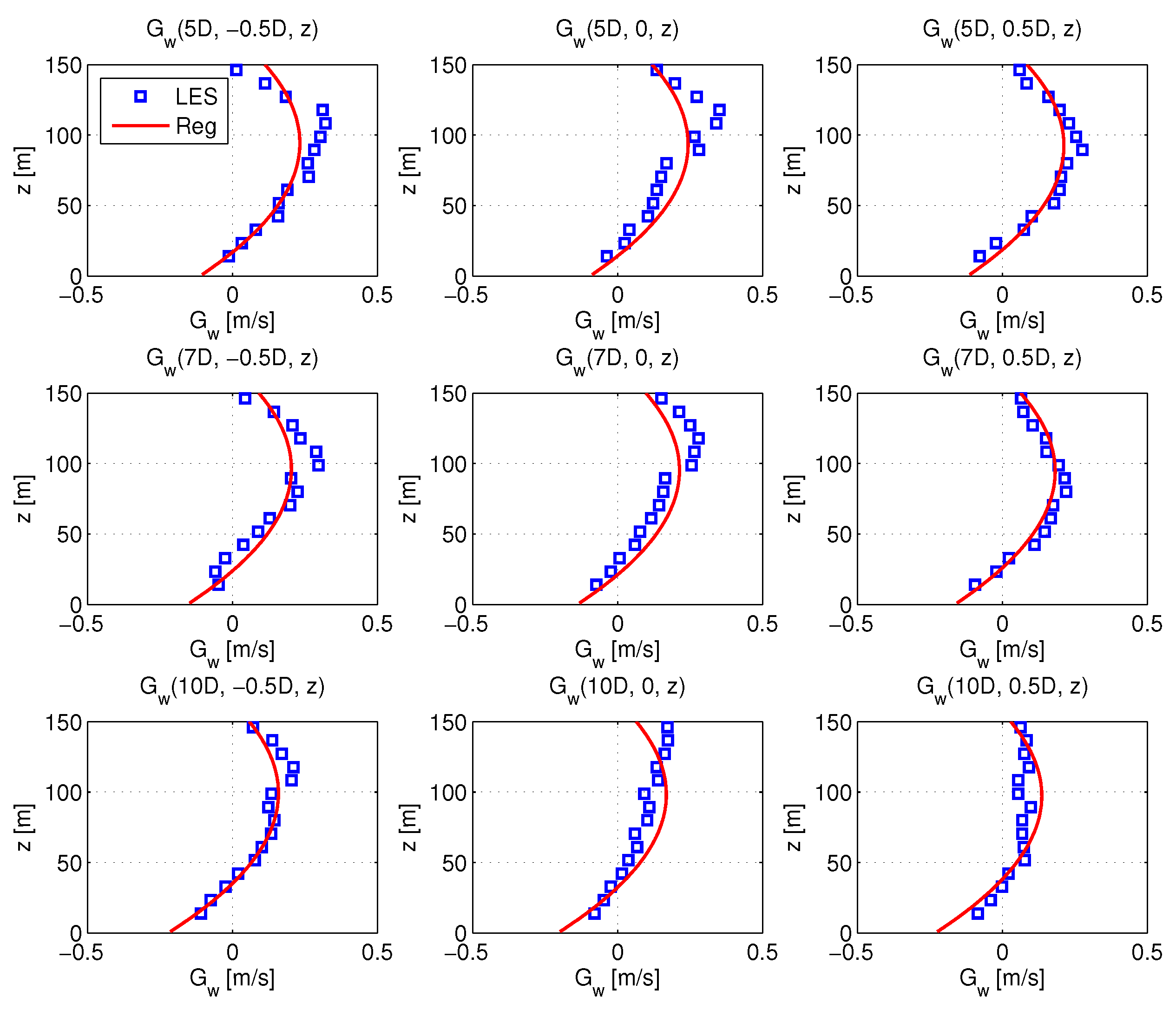
Figure 24.
Spatial variation of : LES versus regression-based estimation.
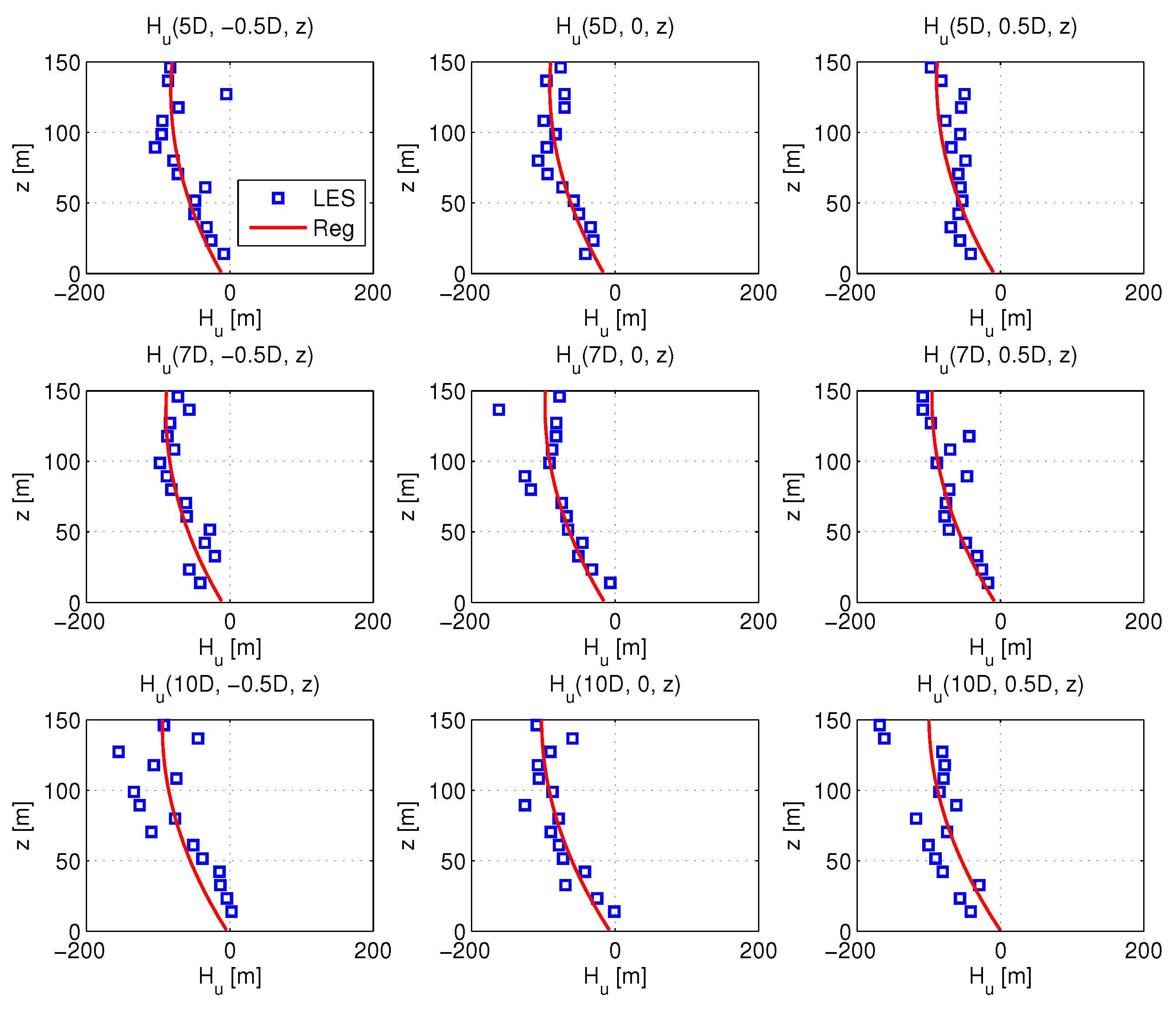
Figure 25.
Spatial variation of : LES versus regression-based estimation.
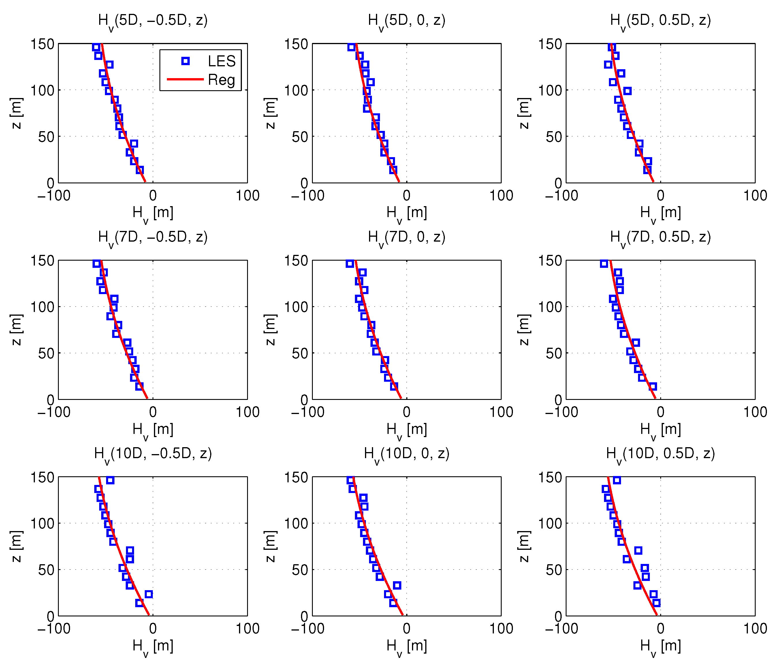
Figure 26.
Spatial variation of : LES versus regression-based estimation.

Figure 27.
Spectra of turbine loads from simulated free stream.
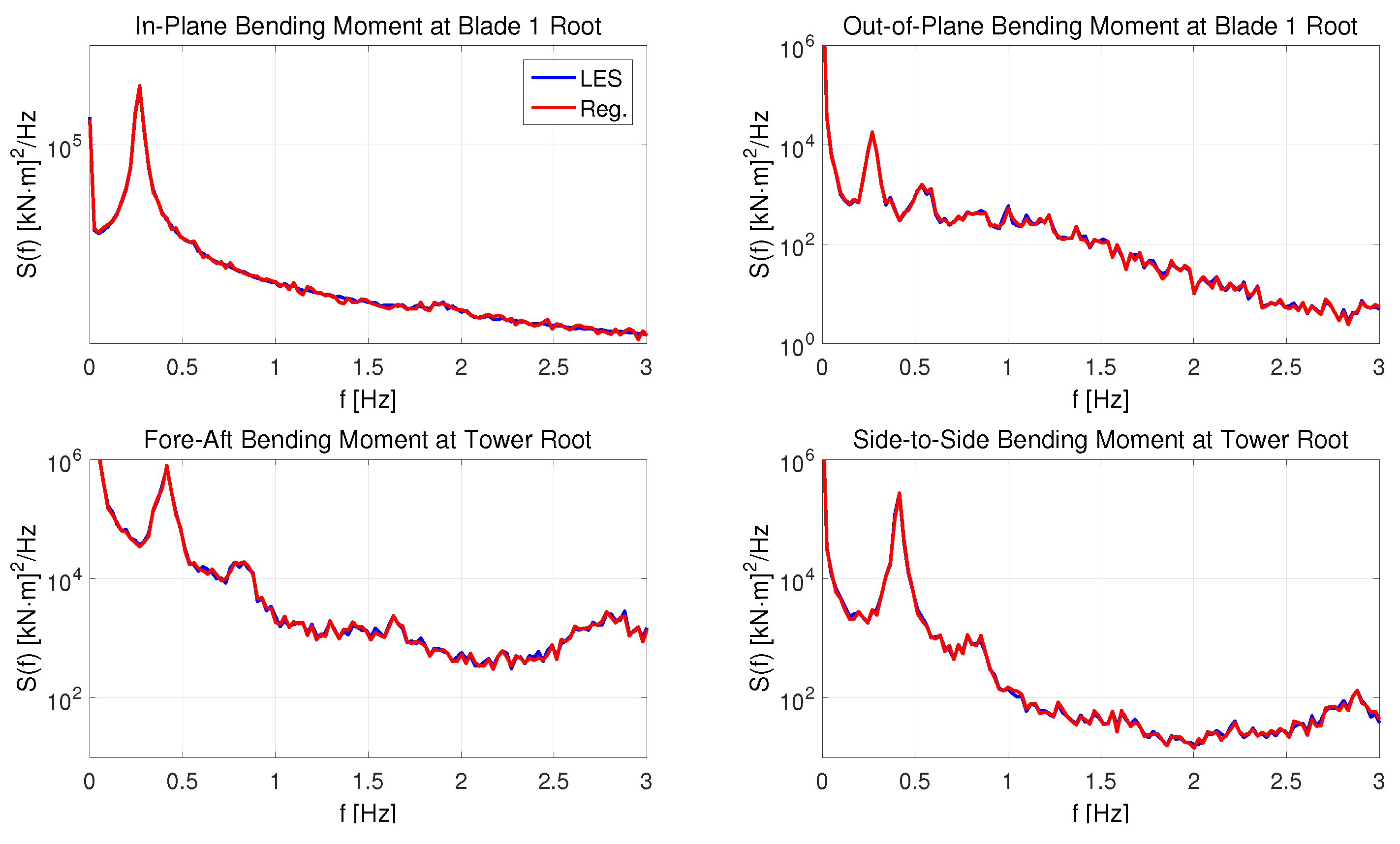
Figure 28.
1-Hz equivalent fatigue loads in the free stream based on LES and on stochastic simulation.
Figure 28.
1-Hz equivalent fatigue loads in the free stream based on LES and on stochastic simulation.
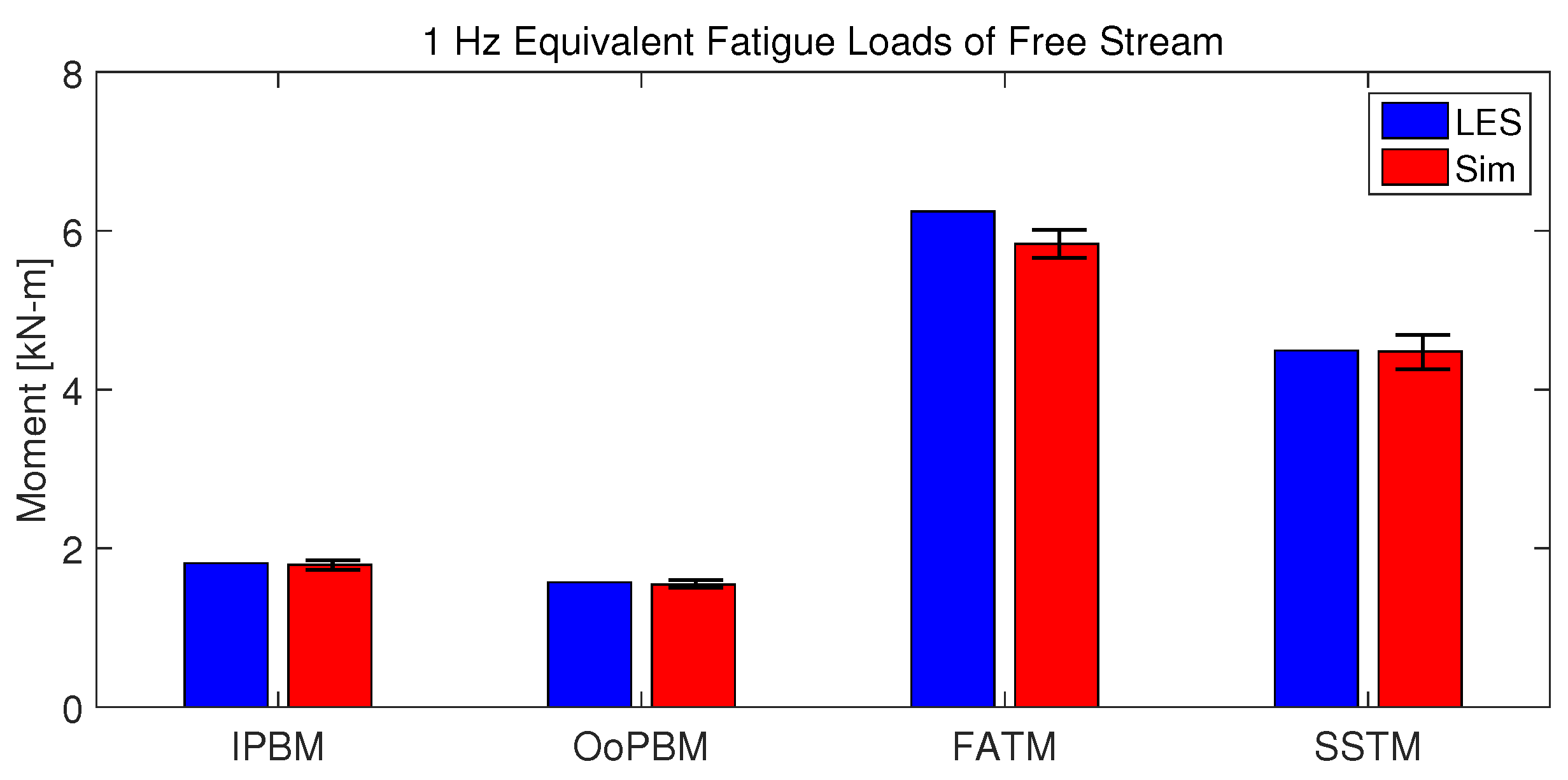
Figure 29.
Power spectra of turbine loads in the free stream and wake based on LES.
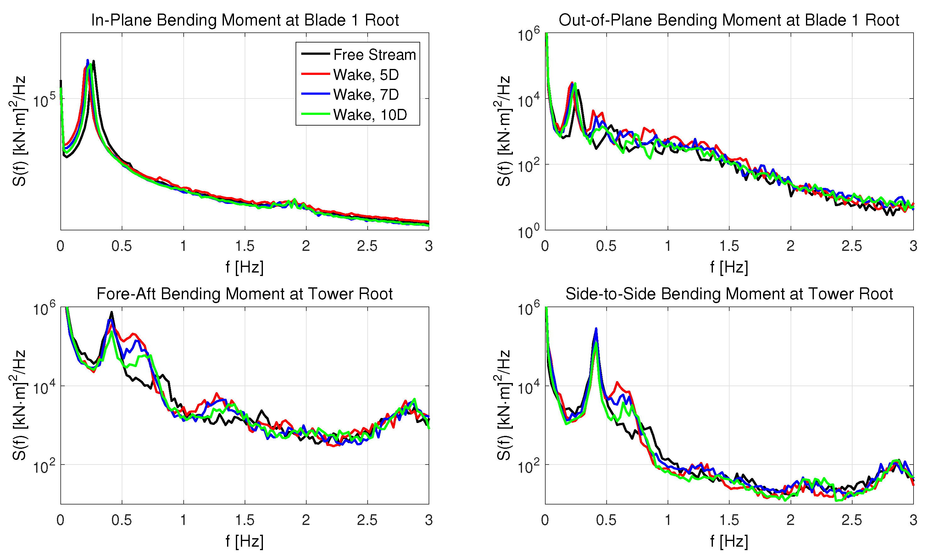
Figure 30.
Normalized 1 Hz equivalent fatigue loads of wake.

Figure 31.
Power spectra of turbine loads in the wake at based on LES and the stochastic model.

Figure 32.
Power spectra of turbine loads in the wake at based on LES and the stochastic model.
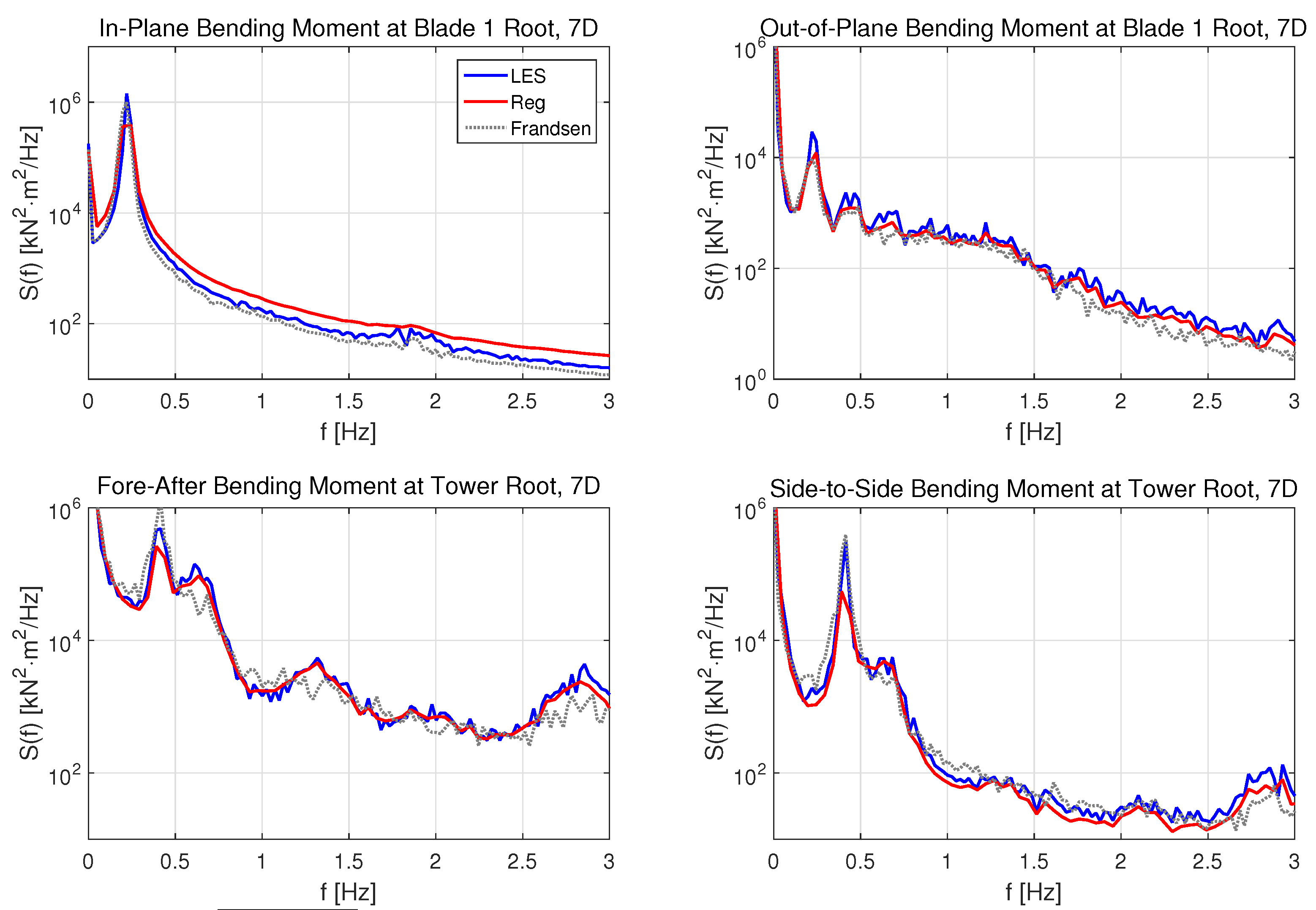
Figure 33.
Power spectra of turbine loads in the wake at based on LES and the stochastic model.

Figure 34.
Normalized 1-Hz equivalent fatigue loads. (a) stochastic simulation; (b) Frandsen model.

Table 1.
Free-stream mean profile regression results.
| Parameter | ||||||
|---|---|---|---|---|---|---|
| Value | 8.19 m/s | 80 m | 0.1489 | −0.088 m/s | 0.0276 | −0.019 m/s |
Table 2.
Free-stream standard deviation profile regression results.
| Parameter | ||||||
|---|---|---|---|---|---|---|
| Value | 0.8045 m/s | −0.0016 | 0.6447 m/s | −0.0016 | 0.5641 m/s | −0.0008 |
Table 3.
Free-stream length scale regression results.
| Parameter | ||||
|---|---|---|---|---|
| Value | 0.2 m | 0.679 m | 0.246 m | 0.221 m |
Table 4.
wake mean field regression results.
| 0.0790 | −0.0026 | −0.1905 | 1.1009 | 0.0245 | |
| −0.0240 | 0.0016 | −0.0941 | −0.0431 | 0.1624 | |
| 0.0038 | −0.0004 | 0.0113 | −0.1792 | −0.0479 | |
| 1.3002 | 0.0117 | −0.0070 | −0.0645 | 0.0176 | |
| 0.0163 | 0.0055 | −0.0018 | 0.2674 | −0.0117 | |
| −0.0789 | 0.0007 | 0.0045 | −0.0066 | 0.0047 |
Table 5.
Coefficients of determination for .
| 0.7772 | 0.7396 | 0.4393 |
Table 6.
Importance of variables in regression.
| p Value | |||||
| 0.1126 | 0.4325 | 0.0029 | 0 | 0.7032 | |
| 0.0548 | 0.0454 | 0 | 0 | 0 | |
| 0.7565 | 0.6171 | 0.4779 | 0 | 0.0028 | |
| 0 | 0.1633 | 0.4090 | 0.0462 | ||
| 0.0764 | 0.0084 | 0.3992 | 0 | ||
| 0 | 0.7447 | 0.1338 | 0.0006 |
Table 7.
wake standard deviation regression results.
| −0.0458 | 0.0012 | −0.0741 | −0.0815 | 0.2488 | |
| −0.0131 | 0.0001 | −0.0090 | −0.0827 | 0.1462 | |
| −0.0149 | −0.0001 | −0.0164 | −0.0859 | 0.0509 | |
| −0.0944 | 0.0030 | −0.0017 | 0.0026 | −0.0078 | |
| −0.0819 | 0.0009 | −0.0016 | −0.0154 | 0.0032 | |
| −0.2299 | -0.0004 | 0.0058 | −0.0037 | −0.0009 |
Table 8.
Coefficients of determination for .
| 0.7030 | 0.7426 | 0.7530 |
Table 9.
Importance of variables in regression.
| p-Value | |||||
| 0.0211 | 0.3517 | 0.0036 | 0 | 0 | |
| 0.1926 | 0.9211 | 0.4837 | 0 | 0 | |
| 0.1551 | 0.8967 | 0.2190 | 0 | 0.0002 | |
| 0 | 0.3690 | 0.6214 | 0 | ||
| 0 | 0.6132 | 0.3323 | 0.2079 | ||
| 0 | 0.8267 | 0.0011 | 0.1308 |
Table 10.
wake integral length scale regression results.
| −6.5286 | 0.3994 | −5.3498 | 22.2887 | −23.9192 | |
| 1.4229 | −0.0950 | 1.4318 | 0.9628 | −18.9324 | |
| −1.9086 | 0.1194 | 1.5593 | 0.8695 | −20.8400 | |
| 25.4228 | 0.4260 | −2.1783 | 18.9252 | −3.2913 | |
| 7.2252 | −0.0491 | −0.7312 | −0.3142 | 0.1277 | |
| 5.3847 | −0.2158 | −0.0998 | 2.1160 | −0.2827 |
Table 11.
Coefficients of determination for .
| 0.5005 | 0.8627 | 0.9121 |
Table 12.
Importance of variables in regression.
| p-Value | |||||
| 0.1789 | 0.2107 | 0.3892 | 0 | 0.0001 | |
| 0.1949 | 0.1880 | 0.3082 | 0.2279 | 0 | |
| 0.0115 | 0.0161 | 0.1065 | 0.1131 | 0 | |
| 0 | 0.6013 | 0.0083 | 0.0997 | ||
| 0 | 0.7902 | 0.0001 | 0.3839 | ||
| 0 | 0.0890 | 0.4347 | 0.9310 |
Table 13.
The WindPACT 1.5-MW wind turbine model.
| Parameter | Value |
|---|---|
| Configuration | 3 blades, upwind |
| Rotor diameter | 70 m |
| Hub height | 84 m |
| Drivetrain | High speed, multiple-stage gearbox |
| Control | Variable speed and pitch control |
| Max. rotor speed | 20.5 rpm |
| Rated wind speed | 11.8 m/s |
| Cut-out wind speed | 25 m/s |
| Tower nat. frequency | 0.387 Hz |
Table 14.
Turbine load statistics in the free stream: Large Eddy Simulation (LES) vs. stochastic model.
Table 14.
Turbine load statistics in the free stream: Large Eddy Simulation (LES) vs. stochastic model.
| Loads (LES/Sim) [kN-m] | IPBM | OoPBM | FATM | SSTM |
|---|---|---|---|---|
| Std.dev | 324/322 | 97/95 | 1042/1035 | 186/184 |
| Max | 594/592 | 1285/1263 | 14130/14088 | 1092/1087 |
Table 15.
Turbine load statistics in the wake: LES model.
| Loads [kN-m] | IPBM | OoPBM | FATM | SSTM | |
|---|---|---|---|---|---|
| Free Stream | Std.dev | 324 | 97 | 1142 | 186 |
| Max | 594 | 1285 | 14130 | 1092 | |
| 5D | Std.dev | 325 | 93 | 825 | 175 |
| Max | 578 | 988 | 9001 | 988 | |
| 7D | Std.dev | 324 | 92 | 964 | 183 |
| Max | 572 | 1008 | 9847 | 974 | |
| 10D | Std.dev | 325 | 93 | 971 | 175 |
| Max | 583 | 1063 | 10710 | 977 | |
Table 16.
Standard deviation and maximum of various turbine loads from stochastic vs. LES waked wind fields vs. Frandsen wake model.
Table 16.
Standard deviation and maximum of various turbine loads from stochastic vs. LES waked wind fields vs. Frandsen wake model.
| Loads (Sim/LES/Frandsen) | IPBM | OoPBM | FATM | SSTM | |
|---|---|---|---|---|---|
| 5D | Std.dev | 324/325/322 | 106/93/111 | 1005/825/1208 | 168/175/192 |
| Max | 568/578/561 | 985/988/917 | 9437/9001/9706 | 846/988/1061 | |
| 7D | Std.dev | 325/324/323 | 104/92/96 | 1064/ 964/1102 | 152/183/185 |
| Max | 566/572/567 | 1028/1008/1016 | 10210/9847/10760 | 816/974/958 | |
| 10D | Std.dev | 325/325/324 | 102/93/96 | 1088/971/1122 | 143/175/183 |
| Max | 569/583/571 | 1063/1063/1076 | 10807/10710/11060 | 826/977/958 | |
© 2017 by the authors. Licensee MDPI, Basel, Switzerland. This article is an open access article distributed under the terms and conditions of the Creative Commons Attribution (CC BY) license (http://creativecommons.org/licenses/by/4.0/).
Share and Cite
MDPI and ACS Style
Moon, J.S.; Manuel, L.; Churchfield, M.J.; Lee, S.; Veers, P.S. Toward Development of a Stochastic Wake Model: Validation Using LES and Turbine Loads. Energies 2018, 11, 53. https://doi.org/10.3390/en11010053
AMA Style
Moon JS, Manuel L, Churchfield MJ, Lee S, Veers PS. Toward Development of a Stochastic Wake Model: Validation Using LES and Turbine Loads. Energies. 2018; 11(1):53. https://doi.org/10.3390/en11010053
Chicago/Turabian StyleMoon, Jae Sang, Lance Manuel, Matthew J. Churchfield, Sang Lee, and Paul S. Veers. 2018. "Toward Development of a Stochastic Wake Model: Validation Using LES and Turbine Loads" Energies 11, no. 1: 53. https://doi.org/10.3390/en11010053
Note that from the first issue of 2016, this journal uses article numbers instead of page numbers. See further details here.