Improvement of Shade Resilience in Photovoltaic Modules Using Buck Converters in a Smart Module Architecture


Copernicus Institute, Utrecht University, Heidelberglaan 2, 3584 CS Utrecht, The Netherlands
*
Author to whom correspondence should be addressed.
Energies 2018, 11(1), 250; https://doi.org/10.3390/en11010250
Submission received: 13 December 2017
/
Revised: 16 January 2018
/
Accepted: 17 January 2018
/
Published: 19 January 2018
(This article belongs to the Special Issue PV System Design and Performance)
Abstract
:Partial shading has a nonlinear effect on the performance of photovoltaic (PV) modules. Different methods of optimizing energy harvesting under partial shading conditions have been suggested to mitigate this issue. In this paper, a smart PV module architecture is proposed for improvement of shade resilience in a PV module consisting of 60 silicon solar cells, which compensates the current drops caused by partial shading. The architecture consists of groups of series-connected solar cells in parallel to a DC-DC buck converter. The number of cell groups is optimized with respect to cell and converter specifications using a least-squares support vector machine method. A generic model is developed to simulate the behavior of the smart architecture under different shading patterns, using high time resolution irradiance data. In this research the shading patterns are a combination of random and pole shadows. To investigate the shade resilience, results for the smart architecture are compared with an ideal module, and also ordinary series and parallel connected architectures. Although the annual yield for the smart architecture is 79.5% of the yield of an ideal module, we show that the smart architecture outperforms a standard series connected module by 47%, and a parallel architecture by 13.4%.
1. Introduction
It is now commonly acknowledged that fossil fuel-based generation presents serious challenges to the environment, in terms of global warming, climate change, and society at large. It is also commonly acknowledged that renewable energy sources (RES) are viable, clean, and efficient alternatives. Amongst the RES, photovoltaic (PV) systems, which are maintenance and pollution free [1,2,3], have been increasingly used as the main source of power generation in both standalone and grid-connected residential and large-scale systems [3]. Every year the solar industry is breaking new records and the global PV market grew significantly to at least 74.4 GW in 2016 [4]. Moreover, in 2016 solar installations contributed 39% of all new electric generating capacity, for the first time more than all other technologies [5].
Energy harvesting from a PV module under uniform irradiation is simply possible by connecting it to an inverter that implements a maximum power point tracking (MPPT) algorithm along with a DC-AC converter. The most frequently used MPPT methods are gradient descent based methods such as perturb and observe (P&O) and incremental conductance (Inc. Cond); these conventional methods are also denoted as hill climbing algorithms [6]. MPPT algorithms are used to control the converter as an interface between the PV module and the grid and/or load. However, irradiation is not always uniform, and partial shading (PS) conditions lead to module mismatches, which is one of the main issues in urban PV installations due to adjacent obstacles in buildings. This will become even more relevant in building-integrated PV, in particular façade-based systems. Partial shading has a strongly non-linear effect on PV outputs [7]. For a series connected PV module system even with a highly efficient MPPT algorithm partial shading may lead to almost 70% of power loss [8]. Based on the module architecture and system topology, a power-voltage (P-V) curve as a PV module characteristic may change from a concave curve with one global maximum (GM) to a curve with multiple local maxima, of which one will be the global maximum. The main challenge for this partial shading condition is to find the GM for maximum performance. The aforementioned conventional MPPT algorithms may not perform well under PS conditions. It is possible for conventional algorithms to be trapped on a local maximum [9,10]. Many MPPT algorithms have been proposed for the PS condition [11,12,13,14,15], however they are complicated and/or require long tracking times.
An alternative way to mitigate the PS effects in a PV system is to change the configuration of the PV system depending on the variation of the shading pattern. PV system configurations have been suggested to be changed via different interconnections of individual PV modules, which are typically from one of the following configurations: (i) series-parallel (SP); (ii) total-cross-tied (TCT); and (iii) bridge-linked [9,16]. In [17] an electrical array reconfiguration is proposed, which uses a switching matrix for changing the position of the PV modules and find the best configuration between those. This method is at the module level and implemented to maximize the available DC power by grouping modules with similar shading patterns.
Dynamic reconfiguration methods that are implemented on the module level and depend on an optimization algorithm may be very complicated and may perform at a sluggish pace. As curves with multiple maxima occur because of the effect of bypass diodes (BPD), one way to mitigate PS effects is to divide the module into groups of a small number of cells, while we note that the best option is to have one diode for each cell. Although more BPDs lead to shade-resilient modules [18], increasing the number of BPDs increases the number of local maximum peaks and subsequently a more accurate and complicated MPPT algorithm is required to find the GM of the module. Moreover, the efficiency losses with the BPDs are still significant [19]. One way to overcome this problem is to replace the ordinary BPD with an active BPD, which in fact is an electrical circuit consisting of Metal-Oxide-Semiconductor Field-Effect Transistors (MOSFETs).
Different configurations for module integrated electronics can be categorized in the following groups: (i) Conventional systems, consisting of three BPDs per module and a central converter to change the output voltage level; (ii) Buck converters, to which normal PV modules are connected and thus the output current of the shaded module is to be controlled; (iii) Buck-Boost converters, in which configuration both current and voltage are to be controlled; and (iv) Voltage equalizers, which are a combination of different converter or even bidirectional converters to equalize the voltage by power processing [19,20,21].
In the present study a generic model is developed that can be used for various module configurations and is not limited to number of cells, for instance. It uniquely combines machine learning with system architecture design. In this paper, we employ the method for mitigating the PS condition using the following smart module architecture: a certain small number of solar cells are grouped and connected to a DC-DC buck converter. Connection of the buck converters then makes up the smart module. The converter is used to control the current level and also maximizes the harvested energy from the group of cells. To investigate the shade resilience different shading patterns are modeled. The performance of the smart module is tested under these shading patterns using a full year of measured irradiation data. To have a better understanding about the smart module performance the output of this module is compared with the following PV module architectures: (i) Series connected: an ordinary module with three groups of solar cells in series, there is one BPD for each group of cells to bypass the group in case of shading; (ii) Parallel connected: a module consists of three parallel strings where each string is ended with a blocking diode; (iii) Ideal module with one converter per cell, which is assumed as the ideal reference for comparison of the output of other modules. The model is developed in MATLAB (2017a, MathWorks, Natick, MA, USA). Shading patterns in the simulations contain two different varieties of shading, random and pole shading. To have an accurate understanding about the converter efficiency a least squares support vector machine (LS-SVM, v1.8, K.U. Leuven, Leuven, Belgium) as a machine learning method is implemented to find the exact value of efficiency with respect to input and output voltage and also output current. The same machine learning method is used to calculate the maximum extracted power at different times throughout the year. In all statistical analysis simulations, real data which is extracted from the Utrecht Photovoltaic Outdoor Test (UPOT) facility is used to make the result statistically tangible [22]. Generally, in the smart module architecture a buck converter in parallel with each group of cells controls the shaded groups’ current by leveling down the output voltage of the converter, which simply means that the output current flow in all converters are equal. This strategy helps the shaded groups to perform efficiently while shaded. The series architecture bypasses the shaded groups because of the implemented BPDs. In parallel architecture, the lowest rated voltage determines the voltage output of the whole array, which means wasting power. In both parallel and series architectures, a fraction of power is wasted because of mentioned reasons, but in the smart module architecture all cells, even shaded ones, are producing power efficiently and none of the cells is bypassed.
This paper is organized as follows: Section 2 discusses the principle structure of the smart module electronics including an optimization for the best value of output. Section 3 provides different shading patterns for the architectures under study. In Section 4, results from simulations in Section 3 are discussed. Finally, Section 5 summarizes the potential characteristics of the smart module in terms of shade resilience.
2. Smart PV Module Topology and Design
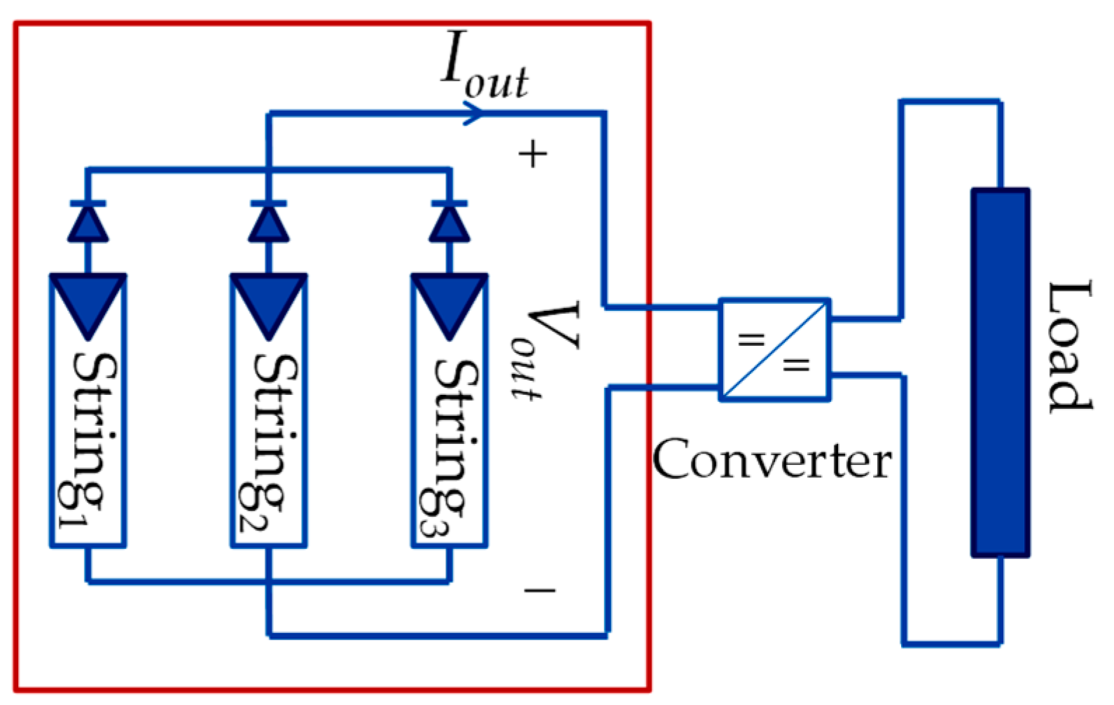
The proposed smart module architecture, as shown in Figure 1, consists of NG groups of cells with ng number of cells in each group.
The total number of cells in a module, N, is calculated as:
PV cells in each group are connected in series and connected to a buck converter. The DC-DC buck converter is controlled via an MPPT algorithm to ensure maximum power extraction from the group. Series connected buck converters in the output of the module is due to current control.
The test module for this simulation study consists of 60 monocrystalline silicon solar cells and we have access to each cell by two connection points for individual analysis. The characteristics at standard test conditions (STC is defined as 1000 W/m2 irradiance, 25 °C cell temperature, Air mass (AM) 1.5 solar spectrum) of the cells are: open circuit voltage (VOC) of 613 mV, short circuit current (ISC) of 7.92 A, maximum power (Pmax) of 3.7 W, and efficiency (η) of 15.4%.
In order to simulate a feasible system, many converters in the market have been studied and a comparison between the most appropriate ones is shown in Table 1. The most suitable converter chosen for the module in this work is the LTM4611 converter from Linear Technology Corporation designs (Milpitas, CA, USA), because of the following reasons: (i) its voltage and current specifications are matched to the small groups of cells in the module; (ii) it has a higher switching frequency compared with Texas Instruments converters, which leads to better performance of the MPPT algorithm; and (iii) no extra element is required for this converter besides the chip itself, which leads to higher efficiency in the complete converter circuit.
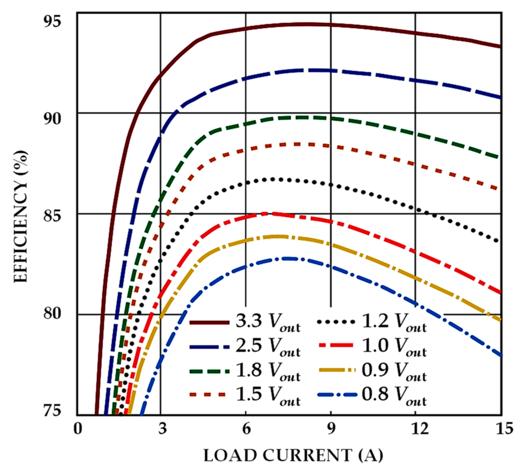
The converter efficiency depends on three different factors: input and output voltage, and output current. In Figure 2, the efficiency of the LTM4611 converter is depicted with these factors as parameters. The important problem is to find the optimum set of variables that lead to the maximum efficiency. To this end, the least squares support vector machine technique is implemented as a standard approach in regression analysis. This method allows to generalize the given data in the datasheet, Figure 2. Therefore, all possible combinations of variables which are necessary for designing are made available in the form of a look-up table. In the following subsection, first the aforementioned method will be introduced and then its implementation for this problem is discussed.
LS-SVM for Efficiency Optimization
The least squares support vector machine method is used to generalize the performance of the LTM4611 buck converter [23]. Let us assume the training set is a set of pre-determined data, where and is the number of elements in data set T. The training set is collected from the datasheet [24]. The LS-SVM uses the training data set to estimate the optimal nonlinear regression function , as shown in Equation (2):
where K represents a so-called kernel function and for this application, the Radial Basis Function (RBF) has been chosen as shown in Equation (3), following [23,25]:
where and the design parameters and b are obtained by solving the matrix-vector equation shown in Equation (4):
Here, represents the identity matrix and is a full matrix with computed elements from the training data as follows:
Parameters and in Equations (4) and (5) are tuning parameters, which can be calculated using different methods, such as k-fold cross-validation, leave one out cross-validation, etc. [23].
The next step in the analysis is to check the feasibility of grouping cells in relation to the converter specifications. Table 2 lists the options under study, showing the calculated voltage at maximum power point for different cases of grouping. From the LTM4611 specification (see Table 1), only case number 5, 6 and 7 are feasible, as the other groupings lead to voltages outside the converter specifications.
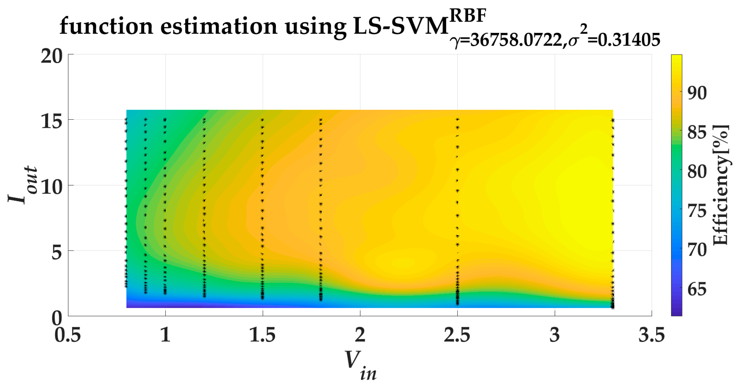
Using all different possible combinations of variables extracted from the buck converter datasheet [24] the efficiency is computed. For instance, Figure 3 depicts the efficiency for input voltage Vin = 5 V, and Figure 4 shows how LS-SVM generalizes the data from Figure 3 to cover all different combinations of and in order to allow computing the efficiency. For the three different case numbers 5, 6 and 7 (Table 2), more information is presented in Table 3.
While the variation in irradiance leads to considerable linear variation in the output current at MPP, it influences the voltage at MPP only slightly (~ln(Isc)). Therefore, as a simplification, the input voltage for buck converter is assumed to be constant having the value as mentioned in Table 3. Although for lower irradiation levels the PV output voltage level in case 7 may not be suitable for this converter specification, all three cases are taken into consideration for comparison. The input current according to the DC-DC buck converter basics is calculated with Equation (6):
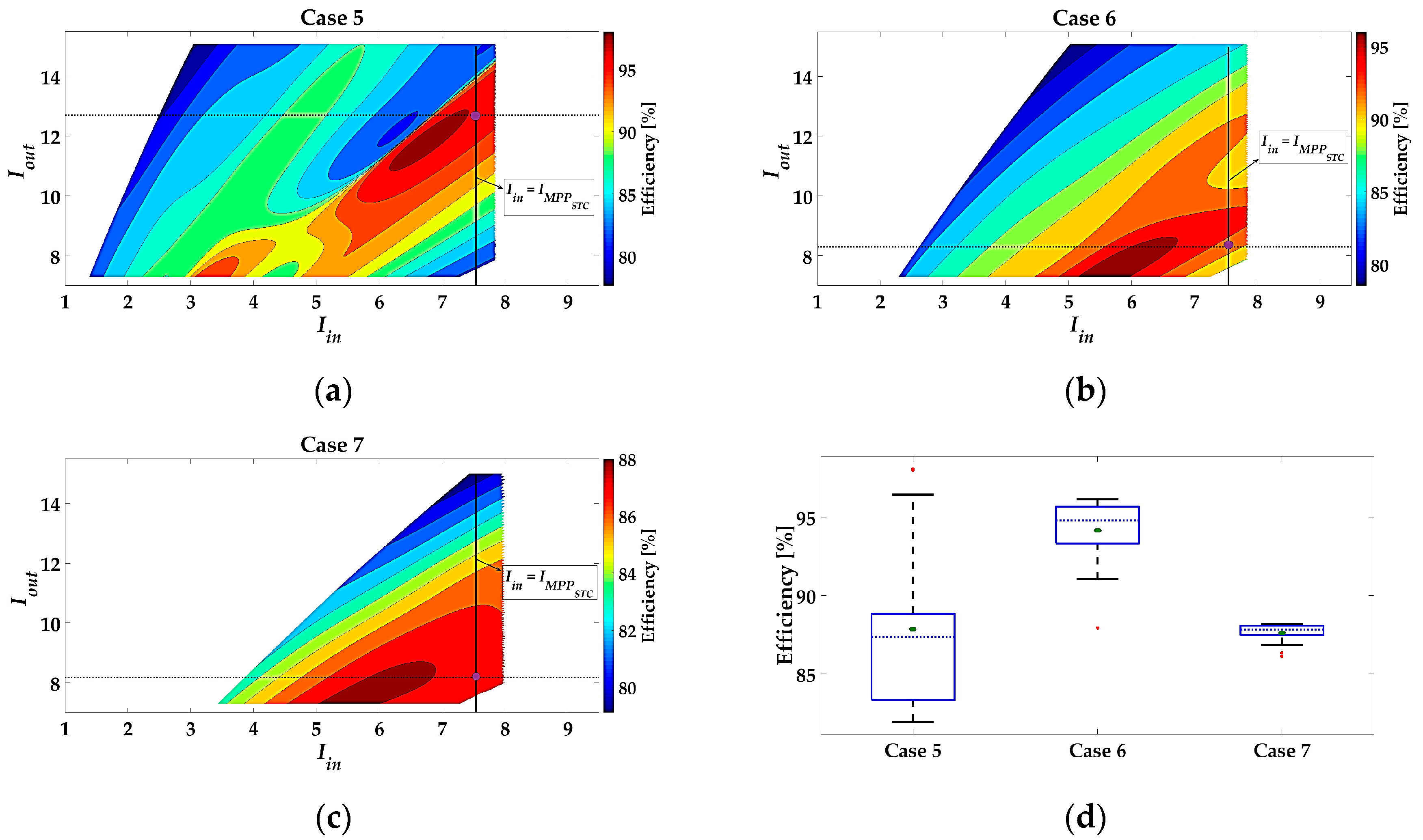
The above-described calculations lead to three contour graphs, one for each case, that are shown in Figure 5a–c. From those, the following can be extracted:
- Referring to the color bars, which are different per case, the highest maximum possible efficiency belongs to case 6, and the lowest maximum possible efficiency belongs to case 7.
- The line (where is the PV output current at STC) is depicted in all figures, thus the best possible efficiency for three cases can be found at intersections of these lines with the contour graphs. Therefore, the best possible efficiencies are 97.74% for case 5, 94.51% for case 6, and 87.69% for case 7.
- It is clear that the best output current should be in the range of 11–13 A for case number 5, where NG = 6, ng = 10, and it should be 8–9 A for case number 6 with NG = 10, ng = 6, and 7–9 A for case number 7 with NG = 15, ng = 4.
- To compare all three cases thoroughly, it is assumed that irradiation level is changed such that the PV output current changes by 50% (). Variation of efficiency in this situation is shown regarding the aforementioned converter output current range in Figure 5d. Although the maximum possible efficiency for case number 5 is higher, the range over which efficiency varies is wider. Also the average values for efficiency (shown in green dots in Figure 5d) indicate that the highest average value belongs to case number 6. That is the reason why case number 6 is chosen for the smart module grouping in this study.
3. Methodology
After designing the architecture and electrical topology of the smart module, let us discuss shading patterns and explain how the module is going to be modeled for this research. We consider the surface of the module to consist of 600 k pixels, which means that each cell has 10 k pixels (ignoring inter-cell distances for simplicity). The irradiation level on pixel p is called and Equation (7) gives the value of this variable:
where is the global horizontal irradiance (GHI) at the pixel and the irradiance at the pixel under the shaded condition.
To calculate the irradiation level on each cell Equation (8) is used, the equation is extracted based on experimental results in a research study by Sinapis et al. [26]:
where is the unshaded fraction of cell C, is the shaded fraction of cell C, NC = 10000 is the total number of pixels of cell C, Nshaded is the number of shaded pixel for cell C, is the global horizontal irradiance, is the diffuse irradiance at the cell C.
The most shaded cell in each group Ni determines the output current of that group Equation (9):
3.1. Different Shading Patterns in This Model
The performance of the smart PV module needs to be tested under realistic shading conditions. In this study two different shading conditions are considered: (1) Random shadow, which might result from the effect of dust, bird droppings, snow, etc.; and (2) pole shadow, which is caused by a static obstacle during daylight, and which is mostly caused by pole shapes, chimneys, dormers, or a part of the building on the roof. Also, these shading conditions can be combined. In the following both types of mentioned shading conditions and the methods for generating them in the model will be described:
- Random shape shading. The characteristics of this shading condition are: (i) probability of occurrence of this shading condition is equal for all surface pixels of the module; (ii) the shape of shading is arbitrary; (iii) random shadows are not necessarily made by solid objects and consequently a transparency factor () is defined as a random function, so that the shadow intensity is randomized; (iv) blur factor () defines how wiped out the shadow borders and edges are. This blur factor is a function of the ratio of diffuse to direct irradiation (); (v) shadow intensity is a function of both the transparency factor and irradiance, see Figure 6a,b.
- Pole shading with the following characteristics: (i) pole shadow position is moving depending on the time of day, which means that the angle of the pole shadow with the module’s x-axis is calculated as a function of time. The length of the pole itself is assumed to be very long so that always the pole shade covers the whole module; (ii) taking into consideration that pole shading occurs only during half of the day due to the sunlight angle, the shape of shading follows the shape of pole; (iii) shading intensity may vary depending on as the pole itself is a solid object; (iv) just as for random shading, the blur factor depends on the ratio of diffuse to direct irradiation, see Figure 6c,d.
The blur factor is a function of the ratio of diffuse to direct irradiation and is determined using a 2D-Gaussian filter, Equation (10):
where x and y are the distances from the origin in the vertical and horizontal axis, and is the standard deviation of the Gaussian distribution. In this model is a function of the ratio of diffuse to direct irradiation: . As an example, the output power for the ten different groups in the module is shown in Figure 6 relative to the power at STC for each iteration: .
3.2. Different Module Calculations
Total output power is computed regarding the module architecture and topology. In this section, the total output power for four different module architectures are mathematically formulated and details are discussed. The model simulates the formulated output power for all of the modules in order to allow for comparisons.
3.2.1. Smart Module
As shown in Figure 1, the smart module topology consists of some groups of PV cells connected in series and connected to a DC-DC buck converter. The DC-DC buck converter is used (i) to control the operating point on the MPP using an MPPT algorithm; and (ii) to control the output current flow. The series connection of buck converters on the output-side forces the converters to work with the same current flow in their output. The MPPT on the input-side of the buck converter controls the operating point to be located at MPP. The buck converter levels down the input voltage, so that the output current could be boosted for the shaded groups with the lower current flow, following Equation (11):
where is the converter efficiency. Total output power for the smart module is computed via
where NG is the number of groups of PV cells, is the maximum group output power at iteration i, and is the MPPT algorithm efficiency. Note that in this model we assume to be constant at 95%. The LS-SVM method is used to calculate by assigning where .
3.2.2. Parallel Strings with Blocking Diodes
The module with parallel-connected strings consists of three parallel strings where each string consists of 20 cells connected in series and ended with a blocking diode, see Figure 7. Normally this topology is implemented for strings of PV modules instead of PV cells. This module is controlled via a central converter with an MPPT algorithm to boost up the voltage level and control the operating point. Therefore, total output power is computed in Equation (13) [27]:
where is the efficiency of the central converter, is the MPPT algorithm efficiency, and the maximum output power at iteration i, is calculated in Equation (14):
Let us assume that the same MPPT algorithm is implemented for all PV module architectures, which has the same efficiency , as in the smart module architecture. The most appropriate converter topology which can be implemented for this module architecture is the boost converter to level up the voltage level, therefore for this study, a buck-boost converter, LT8390, is supposed to be implemented for both parallel and series connected architectures. Figure 8 depicts a variation of efficiency with respect to the input voltage and the output current (load current) for this very high-efficient converter [28]. The same LS-SVM method as mentioned for the LTM4611 is used to map the exact value of efficiency regarding the optimum module operating point.
3.2.3. Standard Module, Series Strings with BPD
The standard module with series-connected strings consists of three series groups of 20 cells, where each group is equipped with one BPD, is shown in Figure 9. Therefore, each group of cells which is shaded would be bypassed via the BPD for preventing cell damage and hot spots and prohibiting the cell to perform as a load instead of a source. Finally, all three groups are connected in series and a central converter may be used to control the operating point. Therefore, total output power is computed using Equation (15):
where the maximum output power at iteration i, is calculated from Equation (16):
where is the voltage of none-bypassed group of cells and is the forward voltage of diodes which bypasses the group of cells with lower current.
It is assumed that the same MPPT algorithm and the same central converter are used as for the parallel-connected architecture.
3.2.4. The Ideal Module Case Study
Let us assume an ideal module, as reference for comparisons. In this ideal module for each cell a DC-DC converter is responsible to level up the current for shaded cells, thus the drop current because of shading is compensated (Figure 10).
The output power from the module is calculated in Equation (17), which is a summation of extracted power from all cell-converter modules:
where is the maximum output power from cell k at iteration i, and are assumed to be 100% and 95%, respectively, for the ideal module architecture.
4. Results and Discussion
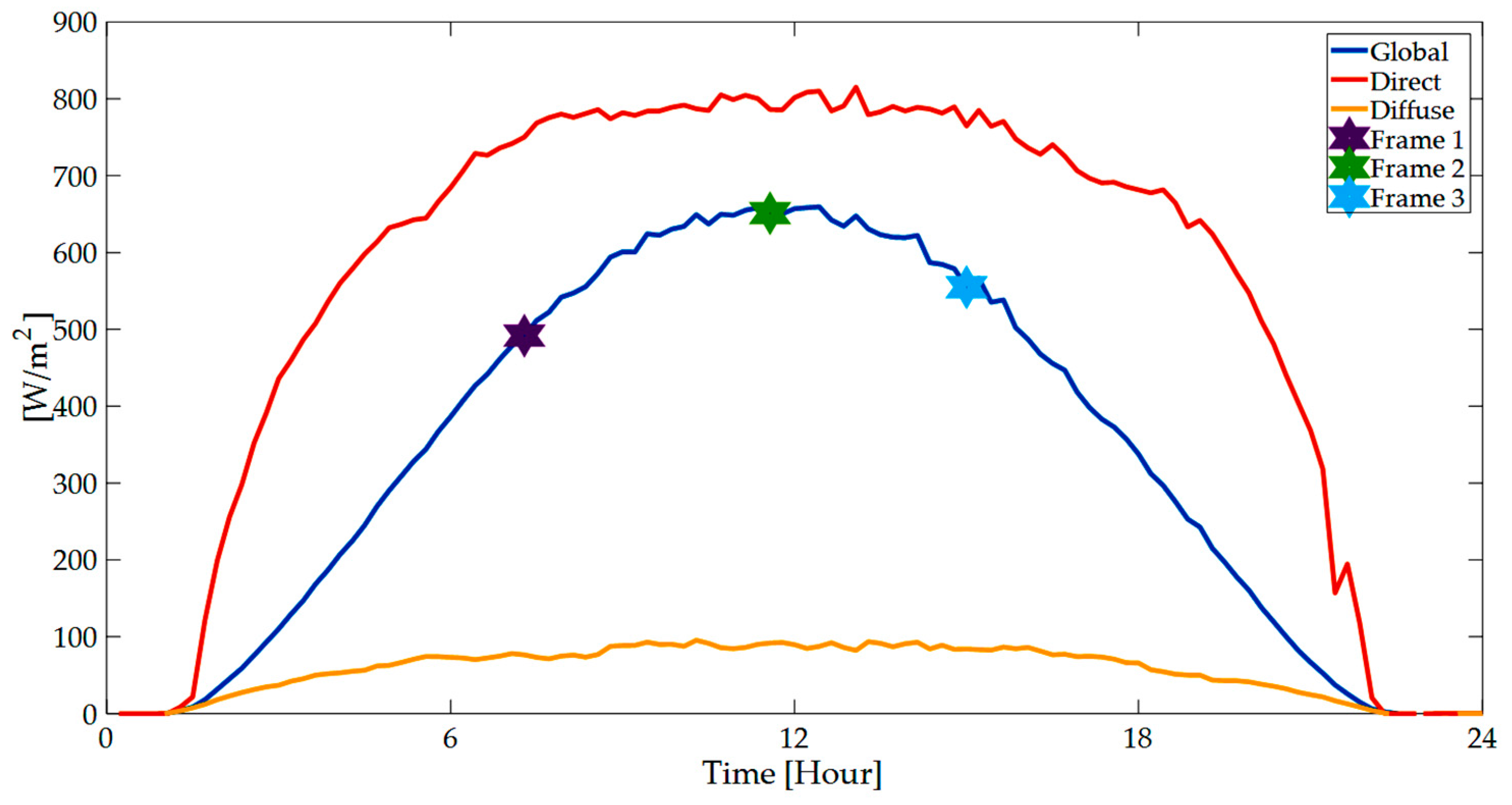
The described model is implemented to simulate the behavior of the smart module as well as the other described architectures under different shading patterns. To understand which architecture is more shade-resilient, the harvested energy during a certain period is computed and compared for all architectures. To this end, experimental irradiance data is used as our model input, which is acquired at the Utrecht Photovoltaic Outdoor Test facility (UPOT) at Utrecht University campus in the center of the Netherlands. Irradiation measurements are done using four EKO MS-802 pyranometers (EKO Instruments, Tokyo, Japan), one EKO MS-401 pyranometer and one EKO MS-56 pyrheliometer; the measurement time is dependent on light intensity and varies from 10 milliseconds to 5 seconds. With these facilities, many variables are being measured every day like irradiation, temperature, humidity, etc. [22,29,30].
For this research available data are (i) global irradiation level; (ii) direct irradiation level; and (iii) diffuse irradiation level for four months, i.e., January, March, June and September 2016. The following steps are followed in the analysis:
- Figure 11 shows recorded data from UPOT at 7 September 2016. Three different time frames of 15 min in length are chosen to be discussed in this section and are pointed out in the figure.
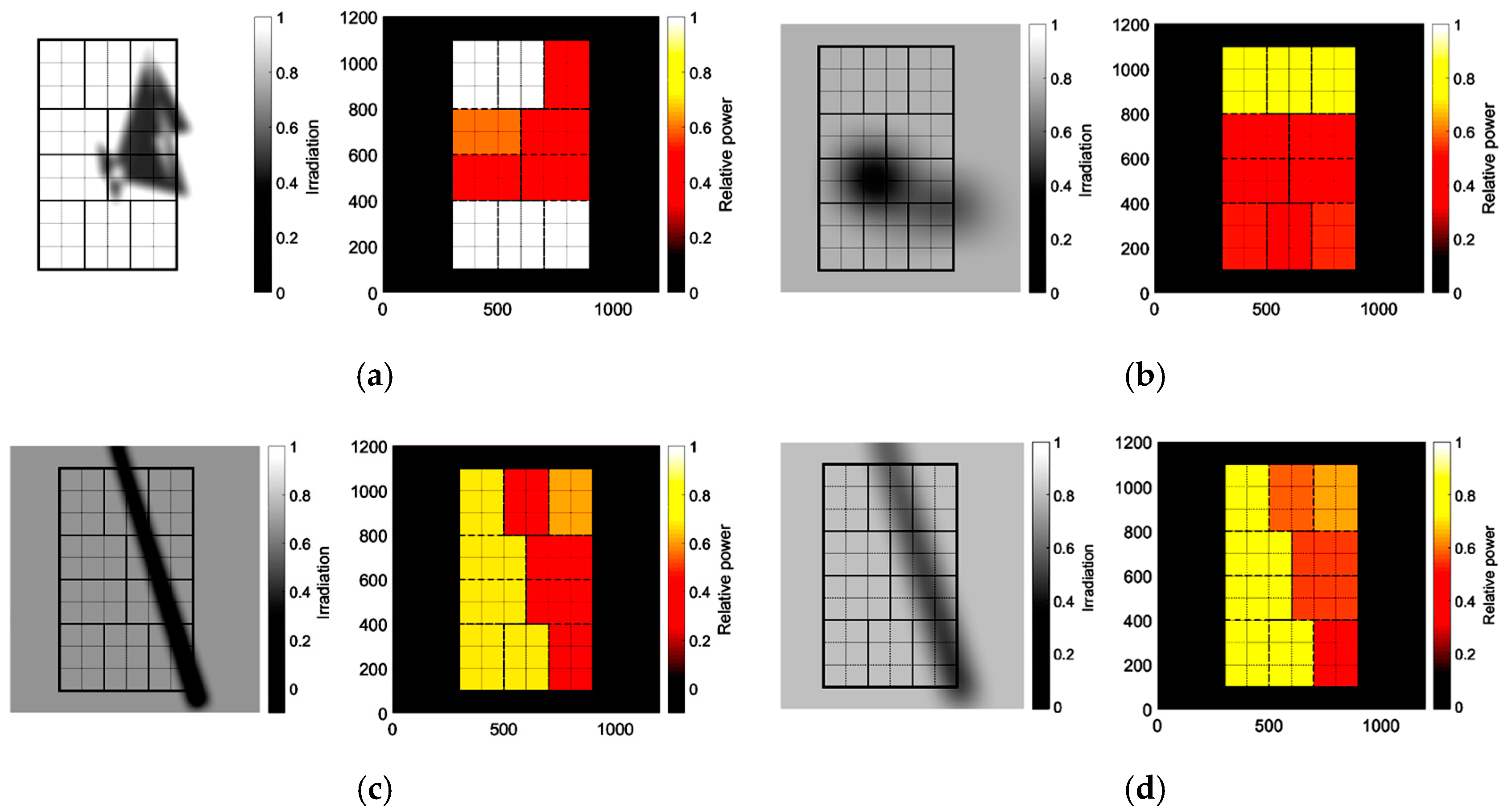
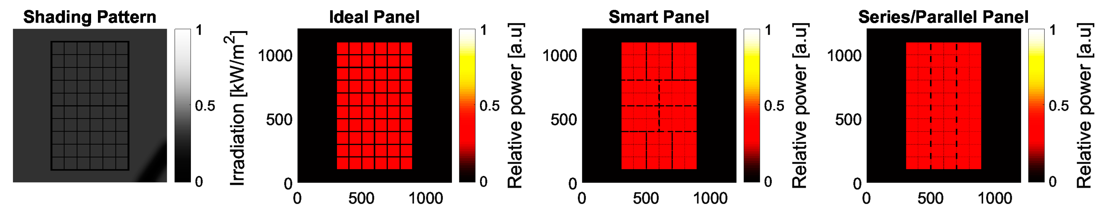
- Generate the shading patterns: following Section 3.1, two types of shadow must be generated depending on obstacles, , , and . Figure 12, Figure 13 and Figure 14 show different shading patterns and their effect on groups of PV cells for different architectures. Unlike in Figure 13 and Figure 14, which only have the effect of pole shadow, in Figure 12 a combination of both pole and random shadows is shown. To observe all shading patterns during this day please refer to Figure S1 in the supplementary section.
- Analysis of the effect of shading patterns on different architectures and cell groups. In this step the effective irradiation level for each group of cells in different architecture is computed precisely.
- Maximum output power at each time frame is calculated using Equations (12)–(17). The output power for three time frames as shown in Figure 12, Figure 13 and Figure 14 is given in Table 4. It is clearly shown that series connected architecture in time frame 1 performs very weak, that is the effect of BPDs in this architecture. The shade pattern in time frame 1 effects on both current and voltage significantly. The group of cells under much darker shadow are bypassed by BPD and current is very low because of the shading.
- Each time frame simulates 15 min of the real world with the assumption of having a constant value of irradiation variables.
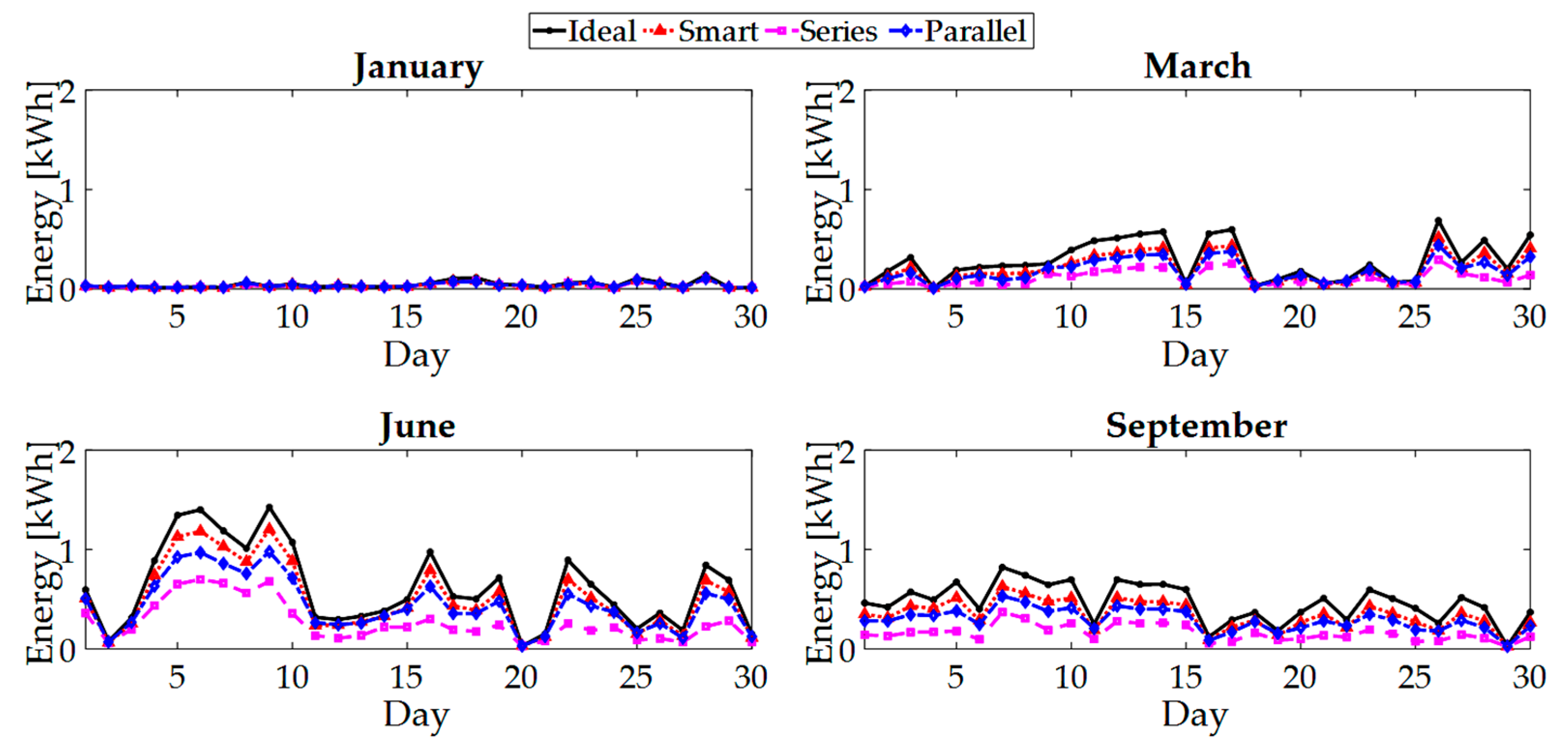
Figure 15 depicts the output energy from different module architectures for different months of the year 2016. The output energy in January is the lowest compared to the other three months. In all three other months, it is clearly shown that the ideal module outperforms all other modules, which is the effect of both the architecture and the 100% and 95% efficiency that is considered for the converter and MPPT algorithm, respectively. For all three months of March, June, and September the second-best performing module is the smart module, followed by the parallel connected and the series connected module. Generally, the drawback of the parallel-connected module is its very low voltage compared to the series-connected module. For designing a practical PV system voltage levels need to be boosted up with a central DC-DC converter and then be controlled to be compatible with the load specifications. In contrast, the series-connected module, which performs worst of all architectures, does not need the boost up the level between load, which thus makes the whole system design easier and more cost efficient.
Figure 16 shows the ratio of output energy from the modules with respect to the output from the ideal module, Equation (18):
Excluding January and the days with very low output energy the smart module performs much better compared to the rest of architectures excluding the ideal module. On the other hand, the series connected module for most of the time generates the lowest amount of energy.
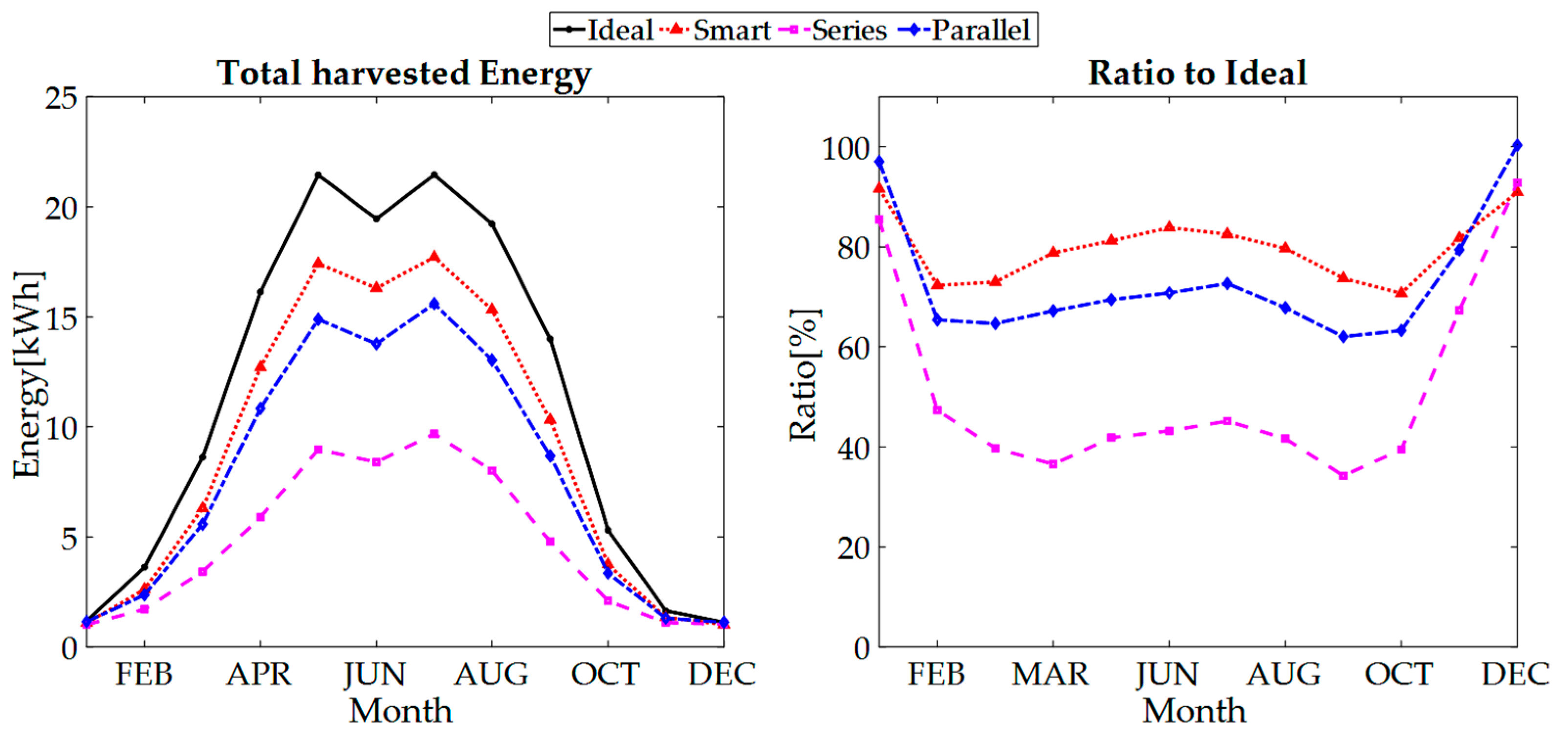
The summation of output energy and the average for the whole year 2016 are depicted in Figure 17. To sum up, the performance of the smart module outperforms all other architectures, except for the ideal module, for all months excluding winter time when the output energy in all types of architecture is almost zero. However, the series connected module as the most ordinary architecture implemented nowadays by most of the manufacturers is performing worst.
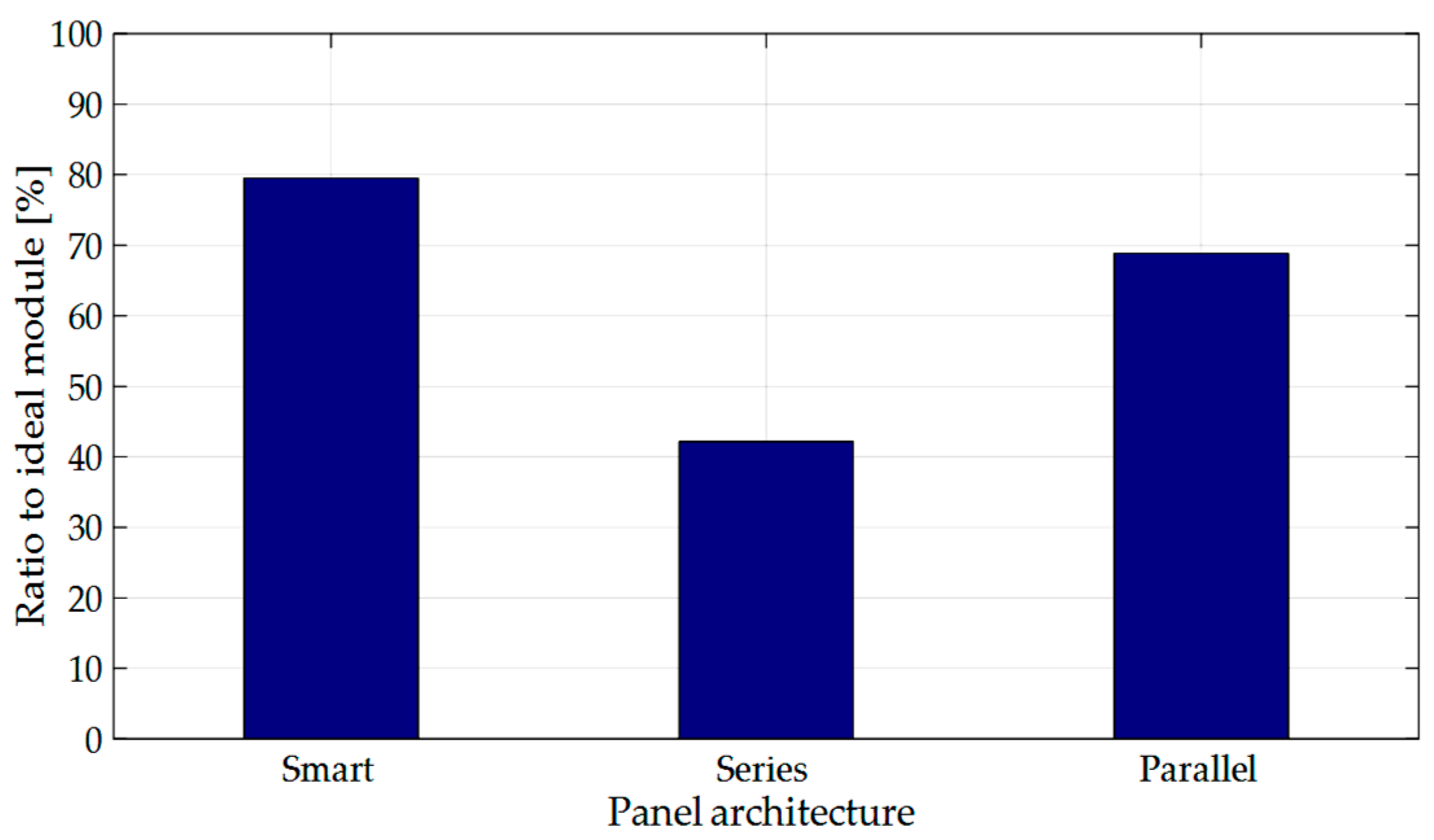
Figure 18 shows the ratio between total harvested energy from smart module, series and connected modules compared to the ideal module. It shows that the smart module harvested almost 79.5% of the energy that the ideal module harvests; the series connected harvested 42.2% and parallel connected yield 68.8% of total module capacity under the same shading patterns.
The method discussed and improved in this study is based on the fact that even small amounts of power which can be produced by cells should be harvested. In other feasible architectures, series and parallel, there are always some energy losses due to the electrical connections. In parallel connection, as the lowest voltage group always determines the module output voltage a fraction of power is lost. As shown in Figure 18 this energy loss is almost 31.2% of total capacity. For series connection, once the BPDs (used for safety reasons), are forward biased in anti-parallel position with shaded groups of cells those groups are bypassed and the module output voltage is decrease. This behavior of BPDs wastes some energy, and this loss is more than half of total capacity: 57.8%. For the smart module, although there is some loss in the electronic circuits due to converter efficiency the final loss compared to the other architectures is reasonably low. According to the results in Figure 18 only 20.5% of energy is lost compared to the ideal module. More importantly, the smart PV module performed 47% and 13.4% better, compared to the series connected and the parallel connected architectures, respectively. The energy loss for the smart module strongly depends on the following factors: (i) optimization of the grouping (number of cells in each group); (ii) converter choosing; and (iii) load current. It should be noted that the actual power rating of the modules, i.e., watt-peak determined under standard test conditions of 1000 W/m2 actually is the same (or very similar) for all three architectures. For unshaded conditions throughout the year, also the energy rating (kWh/kWp) would be the same (or similar). However, for shading conditions, the harvested amount of energy clearly differs. In fact, it could be recommended to develop new standards to test modules under standardized shading conditions.
The addition of electronic elements in a module will lead to additional cost, which should be offset with additional energy harvested under shading conditions. Let us consider the tradeoff between cost and harvested energy comparing both ordinary and smart modules. As the most commonly-used architecture in the market is the series connected architecture, we compare the series connected module with the proposed smart module. According to [31], a public awareness agency funded by the Dutch government, the price of buying a PV system is 1.5 €/W of which panel cost is about half. Thus, a typical panel of 220 W would costs about €170. For transforming an ordinary panel to a smart one we need to purchase 10 micro converters, a microprocessor, and some electronics elements. In this study the designed micro converter is LTM4611, which costs €16, the microprocessor is about €25 and the rest of elements costs roughly €35. To sum up, the final expenditure for a smart panel is about 1.66 times more than an ordinary panel, but as Figure 18 shows under the shading patterns, the annual harvested energy from smart module is 1.89 times more than the series connected. Thus, the economic payback time for a smart module compared to an ordinary series connected module (in shading conditions) is shorter. Note that cost of electronic components are based here on purchasing small amounts. It can be expected that large volume purchases lead to substantial limited additional costs for smart module architectures.
Finally, besides the increased resilience to shading effects, it can be expected that the occurrence of hot spots in smart modules will be limited as well. In a further experimental study, we will investigate that using Infrared (IR) thermography.
5. Conclusions
To mitigate partial shading effects on the performance of PV modules, a generic model is developed that is able to evaluate smart PV module architectures. In this paper the proposed architecture consisted of a number of PV cell groups, and a DC-DC buck converter for a group of PV cells is implemented to amplify the current of shaded groups. This converter was chosen after investigation of characteristics of appropriate micro-converters in the market with respect to the PV cell specifications. This resulted in the choice for the Linear Technology LTM4611 converter. The LS-SVM method was used (i) to generalize the behavior of the converter efficiency; and (ii) to optimize the group size of PV cells. In summary, the optimum grouping for the designed specifications was 10 groups of 6 cells.
After the smart module was designed, the effect of shading patterns was studied. A model for shading patterns was developed with two types of random and pole shadows based on actual measured irradiation data. Simulations demonstrated that the average amount of generated energy of the smart architecture was almost 79.5% of the energy generated by the ideal PV module. Compared with series connected and parallel connected architectures, the smart PV module performed 47% and 13.4% better, respectively. Moreover, the smart module economic payback time compared with the most commonly-used architecture in the market is expected to be shorter.
Supplementary Materials
The following are available online at www.mdpi.com/1996-1073/11/1/250/s1. Figure S1: Shading pattern and different architecture behaviors during the day 7 September 2016.
Acknowledgments
The authors gratefully acknowledge fruitful discussions with Rudi Jonkman and Robert van der Sanden (Heliox), Lenneke Sloof (ECN), and Hamed Yousefi Mesri (UMC). This work is partly financially supported by the Netherlands Enterprise Agency (RVO) within the framework of the Dutch Topsector Energy (project Scalable Shade Tolerant Modules, SSTM).
Author Contributions
S.Z.M.G. and A.C.d.W. conceived and designed the simulations, performed the experiments, and analyzed the data; S.Z.M.G. and W.G.J.H.M.v.S. wrote the paper; W.G.J.H.M.v.S. conceived the project.
Conflicts of Interest
The authors declare no conflict of interest. The funding organization had no role in the design of the study; in the collection, analyses, or interpretation of data; in the writing of the manuscript, and in the decision to publish the results.
Nomenclature
| AM | Air Mass |
| BPD | Bypass diode |
| GM | Global maximum |
| Inc. Cond | Incremental conductance |
| IR | Infrared |
| LS-SVM | Least square support vector machine |
| MPPT | Maximum power point tracker |
| P&O | Perturb and observe |
| PS | Partial shading |
| PV | Photovoltaic |
| P-V | Power-Voltage |
| RBF | Radial base function |
| RES | Renewable energy sources |
| SP | Series parallel |
| STC | Standard test condition |
| TCT | Total-cross-tied |
| UPOT | Utrecht photovoltaic outdoor test facility |
| C | Cell |
| Em | Harvested energy from module m (kWh) |
| Fbl | Blur factor |
| Fshaded | Shaded fraction of cells |
| Ftr | Transparency factor |
| Funshaded | Unshaded fraction of cells |
| GGHI | Global horizontal irradiation (W/m2) |
| Gp | Irradiation level of pixel p (W/m2) |
| Gs | Irradiation level under shadow (W/m2) |
| Iin | Converter input current (A) |
| IG | Output current of group G (A) |
| IMPP_STC | Current at Maximum power point in STC (A) |
| ISC | Short circuit current (A) |
| K | Kernel function |
| ƞ | Efficiency (%) |
| NC | Total number of pixels |
| NG | Number of groups of cells |
| ƞConv | Efficiency of converter (%) |
| ng | Number of cells in a group |
| ƞMPPT | Efficiency of MPPT algorithm (%) |
| Nshaded | Total number of shaded cells |
| p | Pixel |
| Pmax | Maximum output power (W) |
| PMPP | Output power at maximum power point (W) |
| Ptotal | Total output power (W) |
| Rdd | Ratio of diffuse to direct irradiation (%) |
| RE | Ratio of output energy to ideal module (%) |
| Vd_BP | Forward voltage of diode which bypassed group of cells (V) |
| Vin | Converter input voltage (V) |
| Vnon_BP | Voltage of group of cells which are not bypassed (V) |
| VOC | Open circuit voltage (V) |
| Vout | Output voltage (V) |
| σ | Standard deviation |
References
- Rahim, N.A.; Mekhilef, S. Implementation of three-phase grid connected inverter for photovoltaic solar power generation system. In Proceedings of the International Conference on Power System Technology, PowerCon 2002, Kunming, China, 13–17 October 2002; Volume 1, pp. 570–573. [Google Scholar]
- Elsaharty, M.A.; Ashour, H.A.; Rakhshani, E.; Pouresmaeil, E.; Catalão, J.P.S. A Novel DC-Bus Sensor-less MPPT Technique for Single-Stage PV Grid-Connected Inverters. Energies 2016, 9, 248. [Google Scholar] [CrossRef]
- Reinders, A.; van Sark, W.; Verlinden, P. Introduction. In Photovoltaic Solar Energy; John Wiley & Sons, Ltd.: Chichester, UK, 2017; pp. 1–12. [Google Scholar]
- IEA-PVPS. Snapshot of Global Photovoltaic Markets; International Energy Agency (IEA): Paris, France, 2016. [Google Scholar]
- Kreamer, N. SEIA Annual Report 10 Compelling Stories about Solar; Solar Energy Industries Association: Washington, DC, USA, 2016. [Google Scholar]
- Salas, V.; Olias, E.; Barrado, A.; Lazaro, A. Review of the maximum power point tracking algorithms for stand-alone photovoltaic systems. Sol. Energy Mater. Sol. Cells 2006, 90, 1555–1578. [Google Scholar] [CrossRef]
- Papathanassiou, S.A. Energy models for photovoltaic systems under partial shading conditions: A comprehensive review. IET Renew. Power Gener. 2015, 9, 340–349. [Google Scholar]
- Jeyaprabha, S.B.; Selvakumar, A.I. Model-Based MPPT for Shaded and Mismatched Modules of Photovoltaic Farm. IEEE Trans. Sustain. Energy 2017, 8, 1763–1771. [Google Scholar] [CrossRef]
- Bidram, A.; Davoudi, A.; Balog, R.S. Control and Circuit Techniques to Mitigate Partial Shading Effects in Photovoltaic Arrays. IEEE J. Photovolt. 2012, 2, 532–546. [Google Scholar] [CrossRef]
- Mirbagheri, S.Z.; Aldeen, M.; Saha, S. A PSO-based MPPT re-initialised by incremental conductance method for a standalone PV system. In Proceedings of the 2015 23th Mediterranean Conference on Control and Automation (MED), Torremolinos, Spain, 16–19 June 2015; pp. 298–303. [Google Scholar]
- Esram, T.; Chapman, P.L. Comparison of photovoltaic array maximum power point tracking techniques. IEEE Trans. Energy Convers. 2007, 22, 439–449. [Google Scholar] [CrossRef]
- Simoes, M.G.; Franceschetti, N.N.; Friedhofer, M. A fuzzy logic based photovoltaic peak power tracking control. In Proceedings of the IEEE International Symposium on Industrial Electronics, ISIE ’98, Pretoria, South Africa, 7–10 July 1998; Volume 1, pp. 300–305. [Google Scholar]
- Hiyama, T.; Kouzuma, S.; Imakubo, T. Identification of optimal operating point of PV modules using neural network for real time maximum power tracking control. IEEE Trans. Energy Convers. 1995, 10, 360–367. [Google Scholar] [CrossRef]
- Liu, Y.H.; Huang, S.C.; Huang, J.W.; Liang, W.C. A Particle Swarm Optimization-Based Maximum Power Point Tracking Algorithm for PV Systems Operating Under Partially Shaded Conditions. IEEE Trans. Energy Convers. 2012, 27, 1027–1035. [Google Scholar] [CrossRef]
- Mirhassani, S.M.; Golroodbari, S.Z.M.; Golroodbari, S.M.M.; Mekhilef, S. An improved particle swarm optimization based maximum power point tracking strategy with variable sampling time. Int. J. Electr. Power Energy Syst. 2015, 64, 761–770. [Google Scholar] [CrossRef]
- Karatepe, E.; Hiyama, T. Simple and high-efficiency photovoltaic system under non-uniform operating conditions. IET Renew. Power Gener. 2010, 4, 354–368. [Google Scholar] [CrossRef]
- Serna-Garcés, S.; Bastidas-Rodríguez, J.; Ramos-Paja, C. Reconfiguration of Urban Photovoltaic Arrays Using Commercial Devices. Energies 2016, 9, 2. [Google Scholar] [CrossRef]
- Pannebakker, B.B.; de Waal, A.C.; van Sark, W.G.J.H.M. Photovoltaics in the shade: One bypass diode per solar cell revisited. Prog. Photovolt. Res. Appl. 2017, 25, 836–849. [Google Scholar] [CrossRef]
- Olalla, C.; Clement, D.; Rodriguez, M.; Maksimovic, D. Architectures and Control of Submodule Integrated DC–DC Converters for Photovoltaic Applications. IEEE Trans. Power Electron. 2013, 28, 2980–2997. [Google Scholar] [CrossRef]
- Schmidt, H.; Rogalla, S.; Goeldi, B.; Burger, B. Module Integrated Electronics—An Overview. In Proceedings of the 25th European Photovoltaic Solar Energy Conference and Exhibition/5th World Conference on Photovoltaic Energy Conversion, Valencia, Spain, 6–10 September 2010; pp. 3700–3707. [Google Scholar]
- Uno, M.; Kukita, A. Current Sensorless Equalization Strategy for a Single-Switch Voltage Equalizer Using Multistacked Buck–Boost Converters for Photovoltaic Modules Under Partial Shading. IEEE Trans. Ind. Appl. 2017, 53, 420–429. [Google Scholar] [CrossRef]
- Van Sark, W.G.J.H.M.; Louwen, A.; de Waal, A.C.; Schropp, R.E.I. UPOT: The Utrecht Photovoltaic Outdoor Test Facility. In Proceedings of the 27th European Photovoltaic Solar Energy Conference and Exhibition, Frankfurt, Germany, 24–28 September 2012; pp. 3247–3249. [Google Scholar]
- Burges, C.J.C. A tutorial on support vector machines for pattern recognition. Data Min. Knowl. Discov. 1998, 2, 121–167. [Google Scholar] [CrossRef]
- Linear Technology. LTM4611/Typical Application Ultralow VIN, 15A DC/DC µModule Regulator; Linear Technology: Milpitas, CA, USA, 2017. [Google Scholar]
- Suykens, J.A.; Van Gestel, T.; De Brabanter, J.; De Moor, B.; Vandewalle, J. Least Squares Support Vector Machines; World Scientific: River Edge, NJ, USA, 2002; Volume 4. [Google Scholar]
- Sinapis, K.; Tzikas, C.; Litjens, G.; Van den Donker, M.; Folkerts, W.; van Sark, W.G.J.H.M.; Smets, A. A comprehensive study on partial shading response of c-Si modules and yield modeling of string inverter and module level power electronics. Sol. Energy 2016, 135, 731–741. [Google Scholar] [CrossRef]
- Mäki, A.; Valkealahti, S. Power Losses in Long String and Parallel-Connected Short Strings of Series-Connected Silicon-Based Photovoltaic Modules Due to Partial Shading Conditions. IEEE Trans. Energy Convers. 2012, 27, 173–183. [Google Scholar] [CrossRef]
- Linear Technology. 60V Synchronous 4-Switch Buck-Boost Controller with Spread Spectrum 98% Efficient 48W (12V 4A); Linear Technology: Milpitas, CA, USA, 2017. [Google Scholar]
- UPOT—System Layout. Available online: http://upot.nl/system.html (accessed on 7 November 2017).
- Louwen, A.; de Waal, A.C.; Schropp, R.E.I.; Faaij, A.P.C.; van Sark, W.G.J.H.M. Comprehensive characterisation and analysis of PV module performance under real operating conditions. Prog. Photovolt. Res. Appl. 2017, 25, 218–232. [Google Scholar] [CrossRef]
- Milieu Centraal, Prijs en Opbrengst Zonnepanelen—MilieuCentraal. Available online: https://www.milieucentraal.nl/energie-besparen/zonnepanelen/zonnepanelen-kopen/kosten-en-opbrengst-zonnepanelen/ (accessed on 10 January 2018).
Figure 1.
Smart module architecture with ng cells in NG groups with electronic circuits.
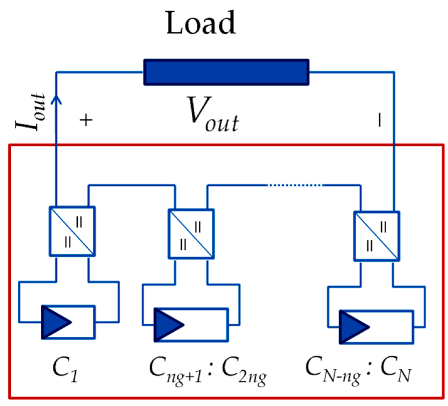
Figure 2.
Efficiency as a function of output (load) current for the LTM4611 converter.
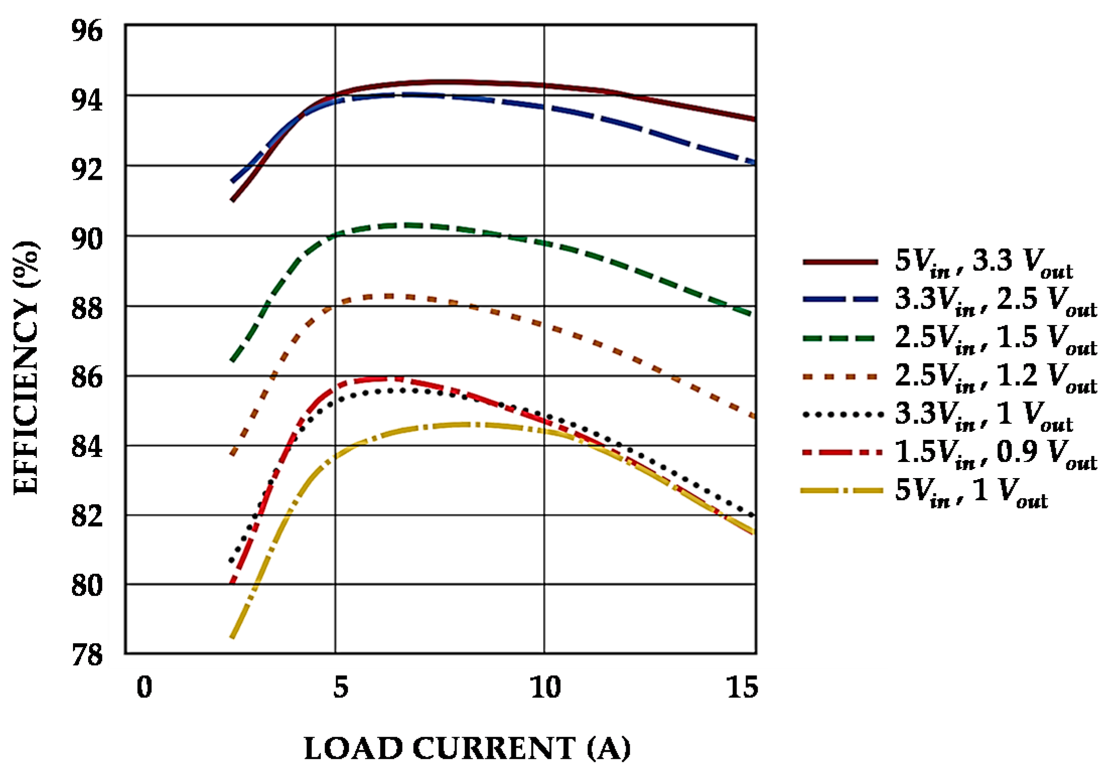
Figure 3.
Efficiency vs Load Current at Vin = 5 V.

Figure 4.
Efficiency for all values of Vin and Iout at Vout = 5 V.

Figure 5.
Contour plots of efficiency as a function of input and output current: (a) case number 5, (b) case number 6, (c) case number 7, (d) efficiency variation with decreasing converter input current for 50%.
Figure 5.
Contour plots of efficiency as a function of input and output current: (a) case number 5, (b) case number 6, (c) case number 7, (d) efficiency variation with decreasing converter input current for 50%.

Figure 6.
Examples of shading pattern, (a) Random shading for higher Rdd, (b) Random shading for lower Rdd, (c) Pole shading for higher Rdd, (d) Pole shading for lower Rdd.
Figure 6.
Examples of shading pattern, (a) Random shading for higher Rdd, (b) Random shading for lower Rdd, (c) Pole shading for higher Rdd, (d) Pole shading for lower Rdd.

Figure 7.
Parallel strings with blocking diode.

Figure 8.
Efficiency vs load current and input voltage for LT8390.
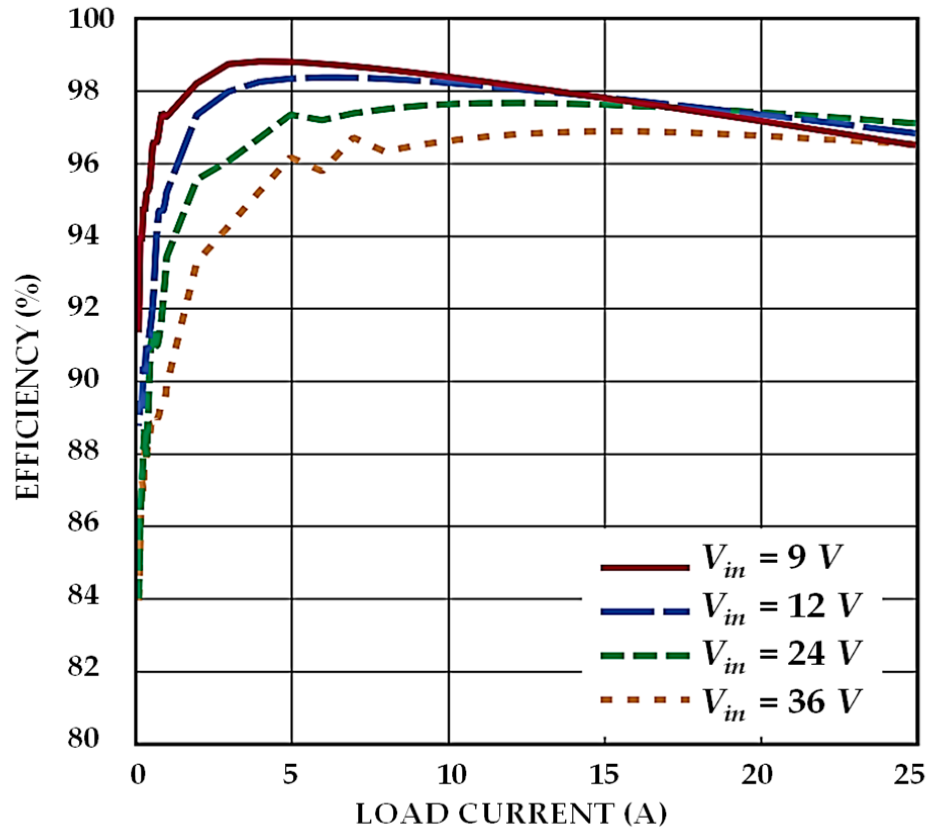
Figure 9.
Standard Module with three BPDs.
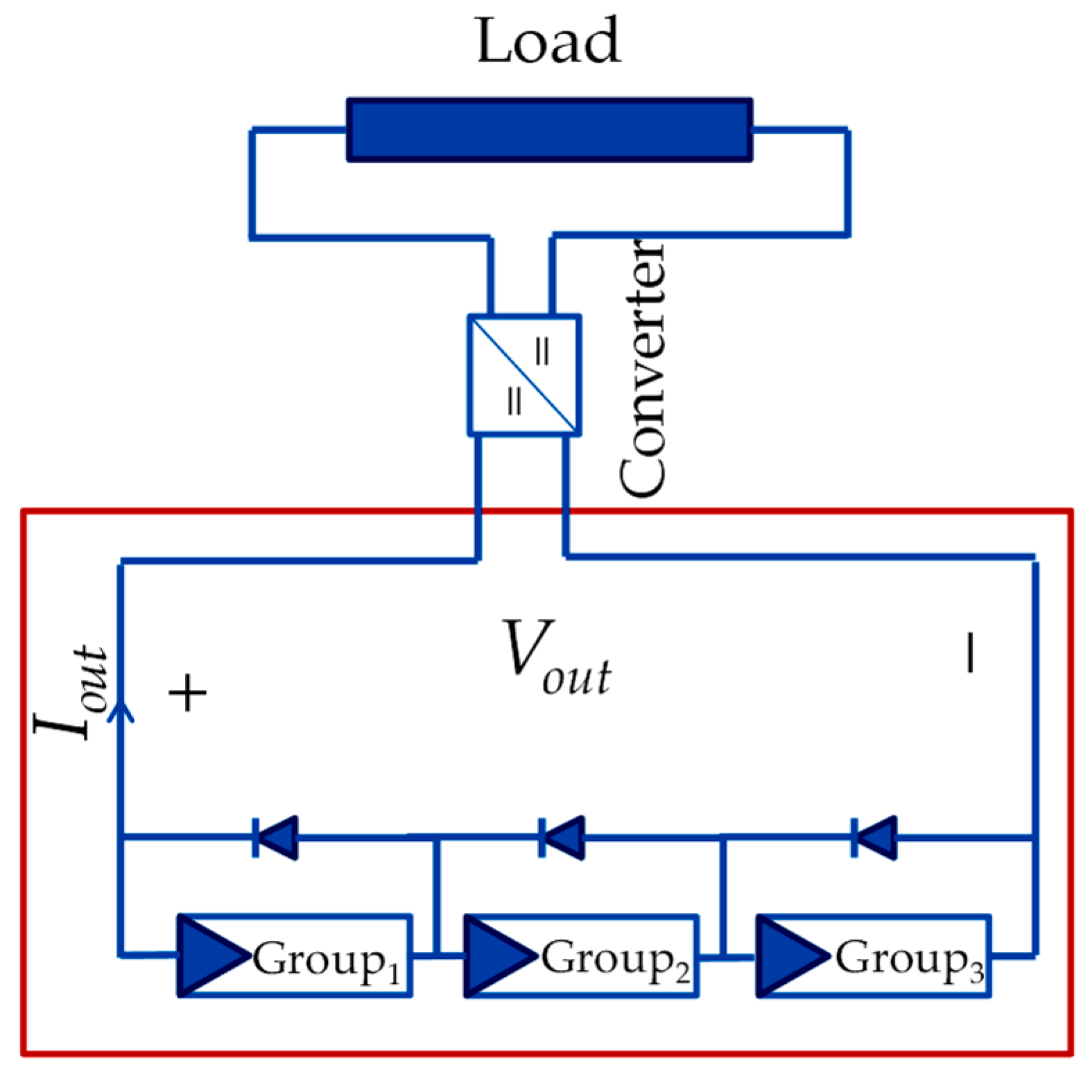
Figure 10.
The ideal module.
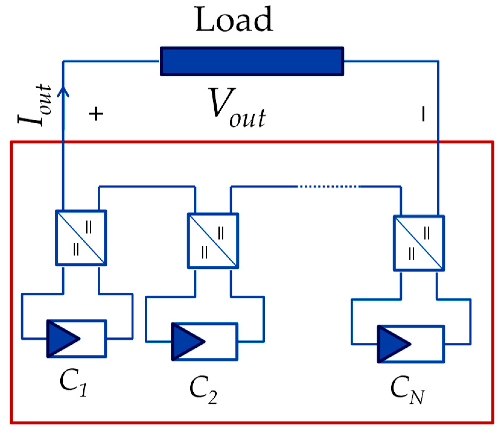
Figure 11.
Global, Direct and Diffuse irradiation levels on 7 September 2016.

Figure 12.
Combined pole and random shading pattern and effect of that on different architectures at time frame 1.
Figure 12.
Combined pole and random shading pattern and effect of that on different architectures at time frame 1.

Figure 13.
Pole shading pattern and effect of that on different architectures at time frame 2.
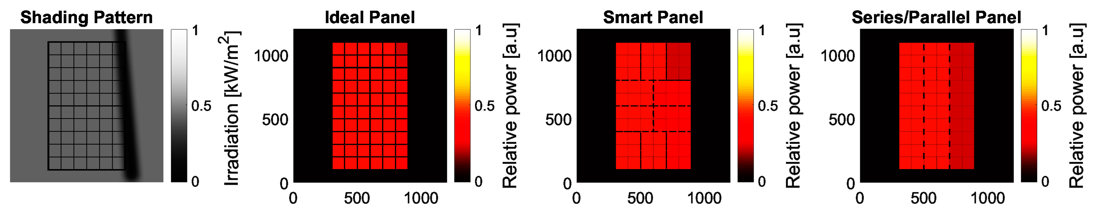
Figure 14.
Pole shading pattern and effect of that on different architectures at time frame 3. Note that the shade is not cast on the panel.
Figure 14.
Pole shading pattern and effect of that on different architectures at time frame 3. Note that the shade is not cast on the panel.

Figure 15.
Harvested energy at four different months of the year 2016.

Figure 16.
The ratio of harvested energy of different architecture compare to ideal module at four different months of the year 2016.
Figure 16.
The ratio of harvested energy of different architecture compare to ideal module at four different months of the year 2016.
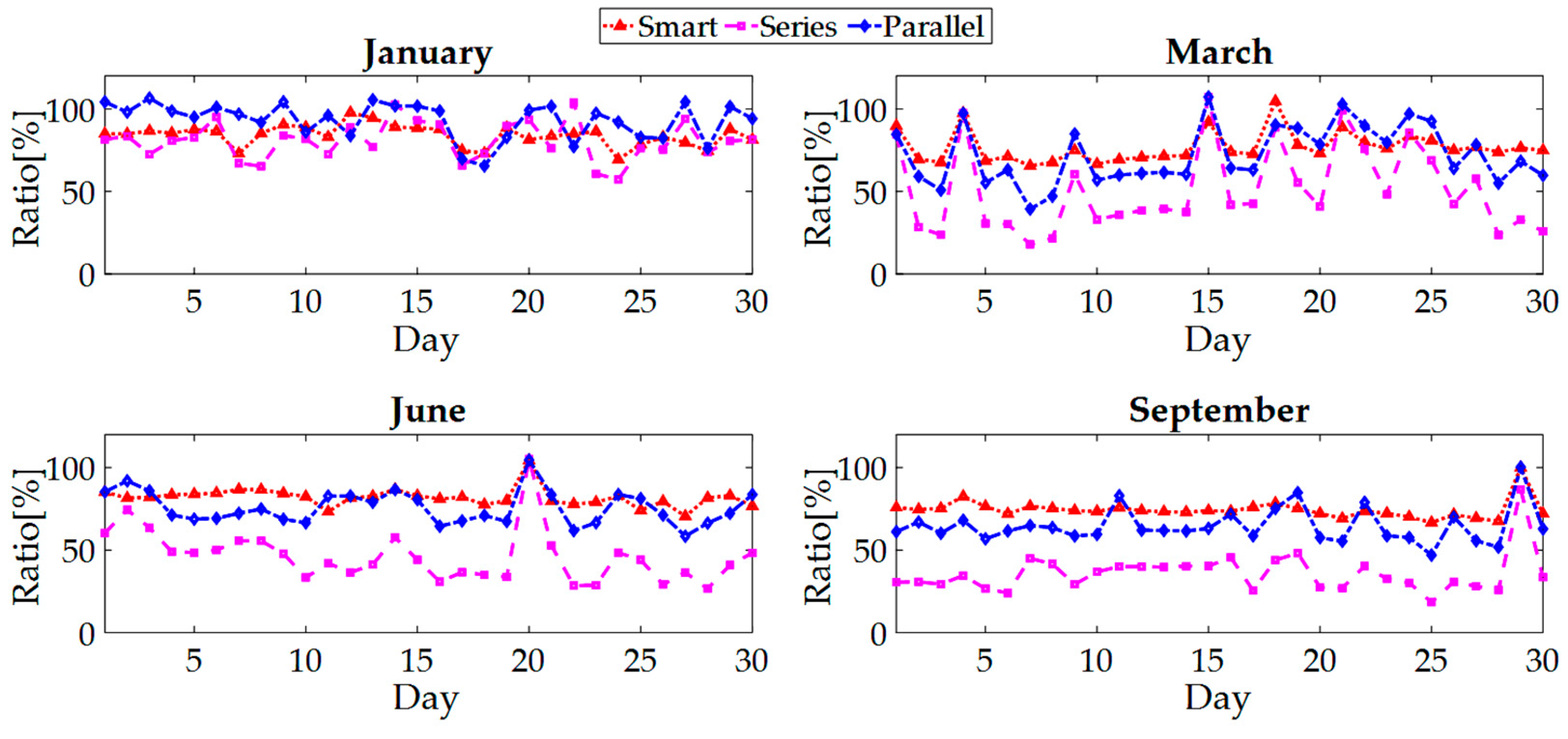
Figure 17.
Perspective of total harvested energy during different months in 2016.

Figure 18.
Ratio of total harvested energy from smart module, series and connected modules compared to the ideal module under shading patterns.
Figure 18.
Ratio of total harvested energy from smart module, series and connected modules compared to the ideal module under shading patterns.

Table 1.
Comparison of different buck converters for the smart module. The colored row indicates the chosen converter.
Table 1.
Comparison of different buck converters for the smart module. The colored row indicates the chosen converter.
| Model | Options | Manufacturer | ||||||
|---|---|---|---|---|---|---|---|---|
| LM2744 | 1 | 16 | 0.5 | 12.8 | 20 | 50 | Ext_Ref_Con 1 | TI 4 |
| LM2747 | 1 | 14 | 0.6 | 12 | 20 | 50 | PbStUp 2 & OpClk 3 | TI 4 |
| LM2745 | 1 | 14 | 0.6 | 12 | 20 | 250 | PbStUp 2 & OpClk 3 | TI 4 |
| LM2748 | 1 | 14 | 0.6 | 12 | 20 | 50 | PbStUp 2 | TI 4 |
| LTC3713 | 1.5 | 36 | 0.8 | 32.4 | 20 | 1500 | Ext_Ref_Con 1 | LT 5 |
| LTC3718 | 1.5 | 36 | 0.7 | 36 | 20 | 1500 | Ext_Ref_Con 1 | LT 5 |
| LTM4611 | 1.5 | 5.5 | 0.8 | 5 | 15 | 835 | Ext_Ref_Con 1 | LT 5 |
1 Ext_Ref_Con: External reference controller, 2 PbStUp: Pre-Bias startup, 3 OpClk: optional clock, 4 TI: Texas Instruments (Dallas, TX, USA).
Table 2.
Overview of cell grouping and buck converter specifications. The colored columns indicate the cases that are selected.
Table 2.
Overview of cell grouping and buck converter specifications. The colored columns indicate the cases that are selected.
| Case Number | 1 | 2 | 3 | 4 | 5 | 6 | 7 | 8 | 9 | 10 |
|---|---|---|---|---|---|---|---|---|---|---|
| # Cells (ng) | 60 | 30 | 20 | 15 | 10 | 6 | 4 | 3 | 2 | 1 |
| # Groups (NG) | 1 | 2 | 3 | 4 | 6 | 10 | 15 | 20 | 30 | 60 |
| Vmpp (mV) * | 29,412 | 14,706 | 9804 | 7356 | 4902 | 2941.2 | 1961.6 | 1471.2 | 980.8 | 490.4 |
| Feasibility | No | No | No | No | Yes | Yes | Yes | No | No | No |
* STC is considered as the highest reference.
Table 3.
Specifications for three cases of grouping at STC.
| Case Number | 5 | 6 | 7 |
|---|---|---|---|
| Number of Cells | 10 | 6 | 4 |
| Open Circuit Voltage (V) | 6.13 | 3.67 | 2.45 |
| Short Circuit Current (A) | 7.92 | 7.92 | 7.92 |
| Current at MPP (A) | 7.54 | 7.54 | 7.54 |
| Voltage at MPP (V) | 4.902 | 2.941 | 1.961 |
Table 4.
Output power in three time-frames.
| Architecture | Frame 1 | Frame 2 | Frame 3 |
|---|---|---|---|
| Ideal Architecture | 48.35 (W) | 84.23 (W) | 116.54 (W) |
| Smart Architecture | 18.49 (W) | 69.00 (W) | 108.85 (W) |
| Series Connected Architecture | 0.84 (W) | 30.95 (W) | 112.35 (W) |
| Parallel Connected Architecture | 4.51 (W) | 62.97 (W) | 113.42 (W) |
© 2018 by the authors. Licensee MDPI, Basel, Switzerland. This article is an open access article distributed under the terms and conditions of the Creative Commons Attribution (CC BY) license (http://creativecommons.org/licenses/by/4.0/).
Share and Cite
MDPI and ACS Style
Mirbagheri Golroodbari, S.Z.; De Waal, A.C.; Van Sark, W.G.J.H.M. Improvement of Shade Resilience in Photovoltaic Modules Using Buck Converters in a Smart Module Architecture. Energies 2018, 11, 250. https://doi.org/10.3390/en11010250
AMA Style
Mirbagheri Golroodbari SZ, De Waal AC, Van Sark WGJHM. Improvement of Shade Resilience in Photovoltaic Modules Using Buck Converters in a Smart Module Architecture. Energies. 2018; 11(1):250. https://doi.org/10.3390/en11010250
Chicago/Turabian StyleMirbagheri Golroodbari, S. Zahra, Arjen. C. De Waal, and Wilfried G. J. H. M. Van Sark. 2018. "Improvement of Shade Resilience in Photovoltaic Modules Using Buck Converters in a Smart Module Architecture" Energies 11, no. 1: 250. https://doi.org/10.3390/en11010250
Note that from the first issue of 2016, this journal uses article numbers instead of page numbers. See further details here.