Study of Time and Meteorological Characteristics of Wind Speed Correlation in Flat Terrains Based on Operation Data

Department of Electrical Engineering, Tongji University, Shanghai 200092, China
*
Author to whom correspondence should be addressed.
Energies 2018, 11(1), 219; https://doi.org/10.3390/en11010219
Submission received: 23 December 2017
/
Revised: 12 January 2018
/
Accepted: 15 January 2018
/
Published: 17 January 2018
(This article belongs to the Section F: Electrical Engineering)
Abstract
:The accurate calculation and characteristic analysis of wind speed correlation (WSC) is the basis of wind farm equivalent modeling, wind power prediction and other advanced applications. It is well known that the accurate calculation of WSC depends on the quality of the raw data, and the WSC of wind turbines is related to spatial, time and meteorological conditions. However, the researches on the statistical analysis of time/meteorological WSC characteristics and the original data quality improvement for WSC calculation are rarely carried out. This paper reviews and redefines the concept and connotation of spatial, time and meteorological WSC. On this basis, a general process is proposed for WSC calculation including data classification, extraction and cleaning. Then the WSC characteristics between wind turbines are analyzed from time and meteorological dimensions based on the actual operation data. In addition, the influence of time WSC and meteorological WSC on wind turbine equivalent modeling and wind power prediction was discussed. The results of case study shows that the proposed general WSC calculation process is feasible and effective; the WSC for different time scales, wind speed ranges and wind directions varies greatly; the spatial WSC cannot characterize the time variability and directionality of the WSC. And the time and meteorological WSC characteristics are of great engineering value to improve the wind turbine equivalent modeling and wind power prediction accuracy, the influence of time scale and meteorological conditions should be considered in the applications of WSC.
1. Introduction
With the rapid development of wind power technology, wind energy has been widely used in the world as a type of renewable energy that is environment-friendly and abundant as well, but its intrinsic properties such as uncertainty and random volatility have brought great challenges to the security and stability of the power system [1,2]. Related researches shows that normally there exists wind speed correlation (WSC) between wind farms or wind turbines with similar geographical locations [3,4]. Theoretically, the study of WSC is not only helpful to analyze the power generation output correlation, but also of great significance for the equivalent modeling of wind farms, wind power prediction, and wind farm cluster control. This can effectively reduce the uncertainty and ambiguity of wind power output and improve the safety and stability of power grid operation [4,5,6,7]. It is of great theoretical significance and engineering application value to carry out relevant research. The study of WSC between wind farms or wind turbines involves WSC calculation, WSC characteristics analysis and its advanced applications. The literature retrieval results show that the current WSC calculation mainly concentrates on mathematical models and methodology, the Pearson correlation coefficient method [8,9] and the optimal parameter Copula function analysis method [9,10] are proposed. When it comes to the characteristic study of WSC, current researches mainly focus on the influence of spatial factors, such as terrain, geomorphology and surface roughness. Literature [11,12] analyzed the WSC in different terrain conditions including hillsides, valleys, airports, pastures and houses, coasts, rugged terrain, the junction between grassland and forest, it is concluded that the WSC is stronger where the terrain is more flat with less obstacle, and the correlation is the strongest at the coast, the weakest in the mountains. Advanced application based on WSC is a research hotspot around the world, mainly researching its applications in wind turbine equivalent modeling [11,12,13], wind power prediction [14,15], power flow calculation [16,17] and wind power integration stability assessment [18,19], etc.
Theoretically, terrain, surface roughness and location, et al. spatial factors are almost constant in a short time [11], but the WSC will be variable and uncertain in different seasons, calendar hours because of the randomness of wind speed and direction [12]. So it is essential to study the influence of seasons, calendar hours and meteorology factors on WSC characteristics [20,21], but little research has been done on the time and meteorology characteristics analysis between wind turbines in a single wind farm.
Moreover, it is apparent that the accurate measure of WSC is the basis of statistical analysis for WSC characteristics and subsequent advanced applications. When analyzing the characteristics of time and meteorological WSC, we need to classify and extract wind speed time series data by time ranges and meteorological factors, which is different from the traditional spatial WSC analysis. The existing spatial WSC calculation process is based on full-time time series data, which cannot classify and extract data at different time and meteorology conditions. That is to say, a new WSC calculation process should be established for the statistical analysis of its time and meteorological characteristics.
In addition, the occurrence of dirty data or data loss in the raw data due to turbine shutdown, sensor failure or other factors will affect the authenticity and objectivity of the WSC. Thus, it’s necessary to exclude dirty data and improve the data quality. Currently, the wind speed data cleaning and its application mainly focus on wind turbine fault diagnosis, oscillation characteristic of wind time series and wind power curve analysis [22,23,24]. Nevertheless, the WSC statistical analysis is based on aligned time series wind speed data, but the wind speed data cleaning methods proposed in references cannot satisfy this requirement. In view of this, this paper proposes a systematic process for WSC calculation including data classification, extraction and cleaning. Then data samples of spatial adjacent wind turbines in flat terrain are selected for statistical analysis of WSC distribution characteristics under different time scales, wind speeds and wind directions. WSC and examples are presented to discuss the influence of time WSC and meteorological WSC on wind turbine equivalent modeling and wind power prediction. This work could supply reference for WSC calculation and its advanced applications.
2. General Calculation Process of WSC Coefficient
2.1. Description of WSC
The influence of spatial terrain, time scale and meteorological conditions should be fully considered when researching the distribution characteristics of WSC. Carrying out WSC research under different spatial, meteorological conditions and time scales has practical engineering value [11,12,13]. The spatial WSC refers to the correlation coefficient based on overall wind speed data, and it is calculated with distinctions of spatial factors; The time WSC is focused on the statistical regularity of correlation coefficient under different time scales, and the operational data should be classified and extracted by different seasons, months, dates and hours; The meteorological WSC reflects the influence of magnitude and direction of wind on the correlation coefficient, and the operational data should be classified and extracted by different wind speed ranges and directions.
The traditional WSC calculation method and process are mainly focused on the spatial correlation analysis, which do not involve the classification and extraction of operation data. Thus it’s not applicable to the statistical calculation of time and meteorological correlation. In view of this, this paper presents a data processing method and correlation coefficient calculation process for the WSC analysis of wind turbines to meet the needs of wind speed spatial, time and meteorological correlation analysis.
2.2. Classification, Extraction and Cleaning & Sorting for Wind Speed Operation Data
Currently, the spatial WSC research is based on overall historical operation data without distinctions of specific factors, which cannot meet the data structure requirements of time and meteorological correlation analysis. In order to describe the differences of wind turbine correlations in different time scales and meteorological conditions, the operational data should be classified and extracted to establish multi-dimension data sets according to specific factors such as seasons, months, dates, hours, wind directions and magnitudes. In addition, it is worth noting that while a wind farm is operating, there must be some dirty data or occurrence of data loss due to wind energy fluctuation, sensor failure, turbine shutdown, or some human factors [25]. The raw data cannot reflect the true operating status of wind turbines and the input-output characteristics between them. Therefore, something must be done with the raw data before analysis.
Obviously, the operation data processing is based on the accurate retrieval of abnormal data. Theoretically, wind speed can be used as a retrieval value to quickly remove the missing data caused by turbine fault or shut down. But when the wind speed is too small or too large, the wind turbines are shut down, in which case there is no engineering application significance to analyze the WSC. In our opinion, statistical analysis of the WSC under the normal power generation state is of practical engineering value for wind farm cluster control and the reducing the influence of wind power integration on the safety and stability of power grid. According to the working principle of wind turbines and the wind farm operation & maintenance regulations, when the input wind speed of a turbine is small (or large), it fails to reach the cut-in wind speed (or reaches the cut-out wind speed), and the output power of the turbine is zero. The output power is also zero when the wind turbine is faulty or shuts down for maintenance. When the wind turbine is in the working state, its output power is greater than zero. Researchers agree that statistical analysis of the WSC between wind turbines in the normal power generation state is of practical engineering value for wind farm cluster control, grid wind power reduction, and power grid security. Therefore, this paper selects the output power of the wind turbine as the retrieval variable of data cleaning, and realizes the cleaning and sorting of the wind speed data. The process is shown in Figure 1.
The output power P being the retrieval mark, we set the rules, as in Equation (1).
where P(t) is the output power at different points of time. If P(t) is greater than zero, the tag value is one; Otherwise, the tag value is zero. Data with a tag value of one are reserved, and those with a tag value of zero are removed.
The steps for wind speed data cleaning are as follows:
• Classification and extraction of operation data
Collect original wind speed and power time series data from the supervisory control and data acquisition (SCADA) system. Next, establish multi-dimensional data sets with distinctions according to the demands of time and meteorological correlation research, such as seasons, months, dates, hours, wind directions and magnitudes, and then extract wind speed data according to the dimensions of the correlation analysis. Wind speed data vacancy filling and time alignment.
There might be data loss caused by turbine shut down or sensor failure in the extracted data. The sampling points with no values are all interpolated with 0 zeros, and the data of different wind turbines complete time alignment. The specific method is as follows:
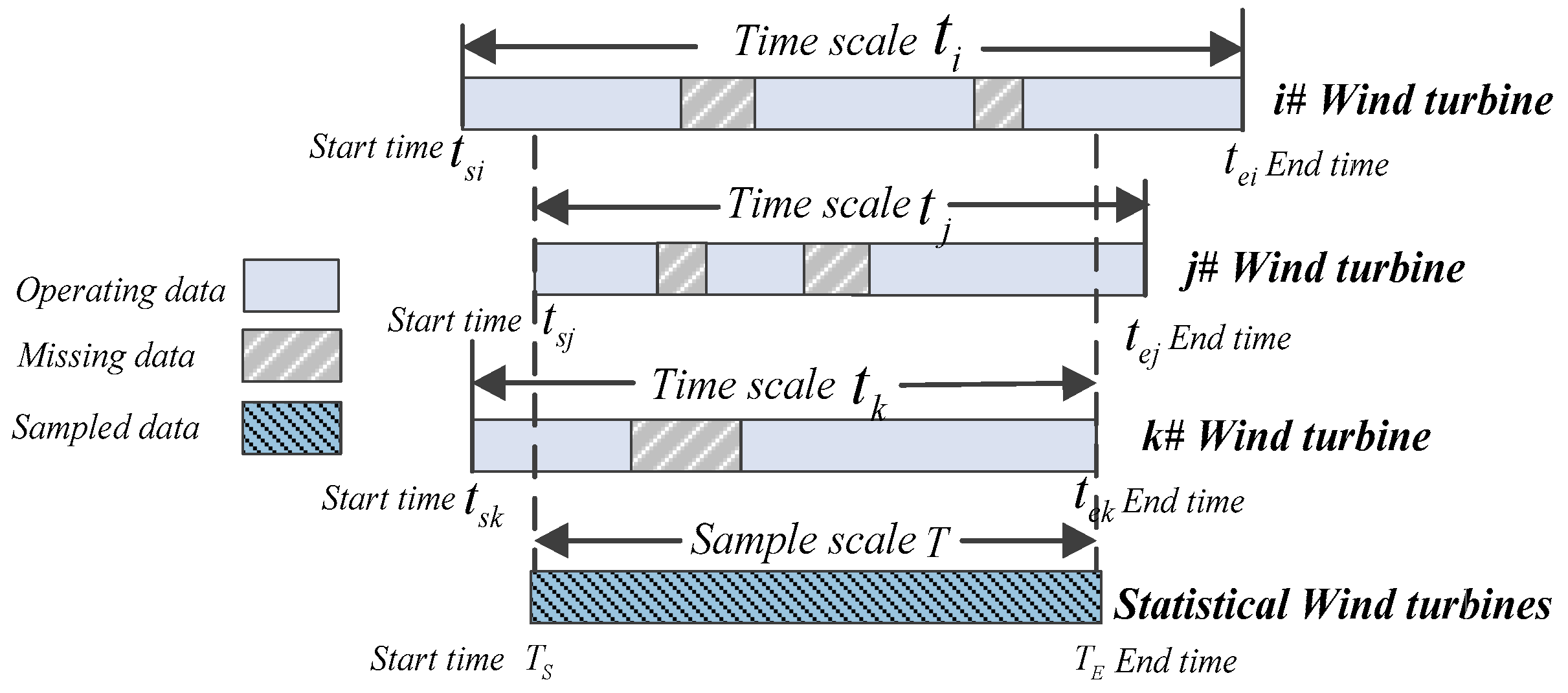
Set wind speed data sampling interval as, the start sampling time is TS and the end time is TE. If there are n wind turbines in a wind farm, the sample time scale selection rule is shown in Figure 2.
It can be seen that the start time TS is the maximum value of all the start times and the end time TE is the minimum value of all the end times, so the common period of wind speed sequence from all wind turbines is selected for correlation analysis. The start time and end time of the selected data sets are calculated as shown in Equation (2). During the sampling period TS~TE, the number of theoretical sampling points for each turbine is shown in Equation (3).
where tsi indicates the start time of the ith wind turbine, tei indicates the end time of the ith wind turbine.
Therefore, the wind speed data sets for correlation analysis can be expressed by a n × m matrix, represented by V, as shown in Equation (4). Similarly, the power output of wind turbines at the corresponding time can also be expressed by a n × m matrix, represented by P, as shown in Equation (5).
where vij is the jth wind speed sampling value of the ith wind turbine, Pij is the power output value of the ith wind turbine at the jth sampling time, in which i = 1, 2 ... n, j = 1, 2 ... m.
Next, the wind speed matrix V and the power output matrix P are assigned. It is firstly judged whether the sampling time t of each turbine belongs to the sampling period [Ts, Te], data over that range are deleted. Then, take the sampling time as the time axis. Fill in the original values of wind speed vij and power output Pij at the corresponding time, and the sampling points with no values are interpolated with 0 zeros. After traversing all the wind turbines, the elements in wind speed sampling matrix V and power output matrix P are all assigned, and wind speed data vacancy filling and time alignment are completed.
• Construction and correction of retrieval matrix for data cleaning and setting
The retrieval and mark rules based on power output time series is established to retrieve the wind speed sequence, in order to obtain the retrieval matrix of each wind turbine. The retrieval rules based on the power output P are as follows: when the power output is greater than zero, the corresponding retrieval value is marked asone in the retrieval matrix; and when the power output is less than or equal to zero, the corresponding retrieval value is marked as zero. Then the data marked one is reserved and the data marked 0 needs to be removed.
If there are n wind turbines in the wind farm and the number of data points collected during the sample period is m, then the power output time series of the ith turbine can be expressed by matrix Pi, as shown in Equation (6). According to the retrieval and mark rules, the retrieval matrix of the ith turbine could be obtained and be expressed by matrix Bi, as shown in Equation (7).
where Pij is the power output value of the ith wind turbine at the jth sampling time, Bij is the jth retrieval value of the ith wind turbine, in which i = 1, 2 ... n, j = 1, 2 ... m.
The modified retrieval matrix is obtained by comprehensive calculation of the retrieval matrix of each wind turbine. For the retrieval matrix Bi of all the wind turbines, the modified retrieval matrix B is obtained by the calculation shown in Equation (8).
where indicates quadrature operation, bj is the jth retrieval value, in which i = 1, 2 ... n, j = 1, 2 ... m.
• Wind speed data cleaning & sorting
According to the modified retrieval matrix, all the sample times marked with 0 in matrix B could be obtained. Sort out and remove the data in wind speed matrix V corresponding to this time series, move up the subsequent data accordingly to fill in the removed sampling points and achieve automatic time alignment, then the wind speed time series can be obtained after data cleaning.
2.3. Calculation Flow of WSC between Wind Turbines
As is known above, the most notable difference between spatial, time and meteorological correlation analysis is the data sets used in the calculation. Spatial correlation analysis is based on overall wind speed data and does not involve data classification and extraction. Dissimilarly, the data for time and meteorological correlation analyze need to be classified and extracted with distinctions of time or meteorological factors. In view of this, a general calculation process is proposed for WSC distribution characteristics analysis. The calculation process of spatial, time and meteorological correlation are unified by the selection of data classification and extraction methods, as is shown in Figure 3.
For the first step, data collection and cleaning. Based on the data of wind speed, wind direction and wind power from the turbine’s SCADA system, construct a data matrix according to time series. An retrieve matrix is constructed with the output power as the retrieve parameter, and abnormal data points are selected by matrix operations. Remove wind speed singular points and complete the automatic time alignment. Then, we obtain the clean and high quality wind speed data after tuning.
For the second step, wind speed series data classification and extraction. The WSC analysis of wind turbines, according to different demands, can be divided into spatial correlation statistics, time and meteorological correlation analysis. While analyzing time and meteorological WSC characteristics, multi-dimensional stratification of the wind speed data is necessary, considering different time periods, wind directions and wind speed ranges. Multi-dimensional wind speed data sets are established in order to provide first-hand data for WSC calculation.
For the third step, WSC calculation. Based on the wind speed data sets after stratification, the WSC between different wind turbines is calculated bases on selected algorithm and the WSC between wind turbines is evaluated quantitatively.
3. Case Analysis
3.1. Wind Speed Data Samples and Their Cleaning & Sorting
In order to ensure the objectivity and accuracy of the statistical analysis results and eliminate the influence of spatial characteristics on time and meteorological correlation analysis, the sample data selection should follow the following principles: (i) The data samples are derived from flat terrains with abundant wind energy resources; (ii) The data samples should have a certain time span, which can reflect the diversity of seasons and meteorological conditions; (iii) The actual operating data should be a preferential selection for the data sample; (iv) Selected wind turbines with high spatial correlation.
Based on the above conditions, the actual operation data of T32 and T33 wind turbines in a wind farm in zhangbei wind power base will be analyzed. Zhangbei wind power base is located in the connecting zone of the North China Plain and the Inner Mongolia Plateau, with flat terrain and abundant wind energy resource. And it is one of the eight million kilowatt class wind power bases in China’s plan. The samples were taken from 1 June 2013 through 1 March 2014, at a 5-min interval. Data book show that both T32 and T33 are SE8215-L3/1500kW type wind turbines, with its cut-in and cut-out wind speeds being 3 m/s and 25 m/s, respectively. Geographically, T32 and T33 are located at the same latitude, and T32 is upstream of T33, with a distance of 700 m apart. Figure 4 shows the wind speed data series of 1000 sampling points (before and after data cleaning) of T32 and T33 in June 2013.
By comparing Figure 4a,b, it can be seen that the sampling points with the wind speed less than 3 m/s are removed after data cleaning and sorting. For sampling points set to be zero in the rough wind speed time series, human interference in the data correlation analysis is avoided through time alignment. Therefore, data cleaning is necessary, and the wind speed series cleaning method and process proposed in this paper are valid, providing objective and accurate data for statistical analysis.
As motioned in above, the Pearson correlation coefficient method and the Copula function theory based method have been proposed to calculate WSC coefficient. Among, the Pearson correlation coefficient, due to its simple calculation and reliability, has obtained extensive applications in describe linear correlation. The Copula function theory, due to its strong nonlinear correlation analysis, is suitable for multivariate coupling correlation description [26]. Considering the WSC distribution has nonlinear properties, the advantages of Copula function calculation method, and the calculation method of the correlation coefficient is not the focus, therefore, the paper calculated WSC coefficient by the Copula function theory based method.
Using spatial WSC to calculate the wind speed data of the sample turbines, it is found that their WSC coefficients before and after cleaning are 0.8697 and 0.9542, respectively. According to correlation judgment criteria, the wind speeds between T32 and T33 are highly correlated, and their correlation after cleaning is obviously better than that before cleaning. The cleaning of wind power data helps to improve the calculation accuracy of the WSC of wind turbines. It can be clearly seen that data cleaning and sorting is necessary for the statistical analysis of WSC distribution characteristics.
3.2. Time and Meteorological WSC Calculation and Characteristic Analysis
As we all know, the wind speed has some other attributes in addition to its magnitude, such as wind time series and wind direction. It is clear that the wind spatial speed correlation statistics can only reflect the magnitude of the wind speed but cannot describe the wind time series and wind direction. However, the subsequent applications and analysis of WSC are based on its time series distribution and meteorological distribution properties. Therefore, it is of great engineering significance to understand the influence of wind energy’s time variability and directionality on the characteristics of wind turbines with different wind speeds, wind directions and time periods [19,20,21]. In view of this, this section will analyze the time and meteorological characteristics of WSC between turbines from multiple dimensions—different months, days, hours and different wind speed ranges and wind direction zones. A comparison will also be made between spatial WSC and time and meteorological WSC to find their differences and impacts on wind farm equivalent modeling and wind power prediction.
3.2.1. WSC at the Monthly Time Scale
The correlation statistics at the monthly time scale are based on the monthly sampling. We examine the monthly WSC coefficients from 1:00 to 4:00 during the period of June 2013 through February 2014. The results are shown in Figure 5.
It can be seen that between June 2013 and December 2013, the WSC coefficient decreased gradually with the month, from 0.95 to 0.55, while it began to climb starting from January 2014.
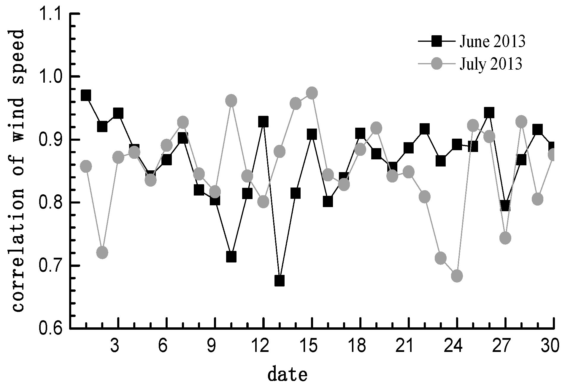
3.2.2. WSC at the Daily Time Scale
In this part, data stratification and analysis are based on the daily sampling. We examine the wind speed series correlation coefficients in June and July 2013, as shown in Figure 6.
It is obvious to see from the figure that the wind speeds of the two wind turbines were highly correlated, but their correlation fluctuated greatly with the date, with a maximum fluctuation of 0.3.
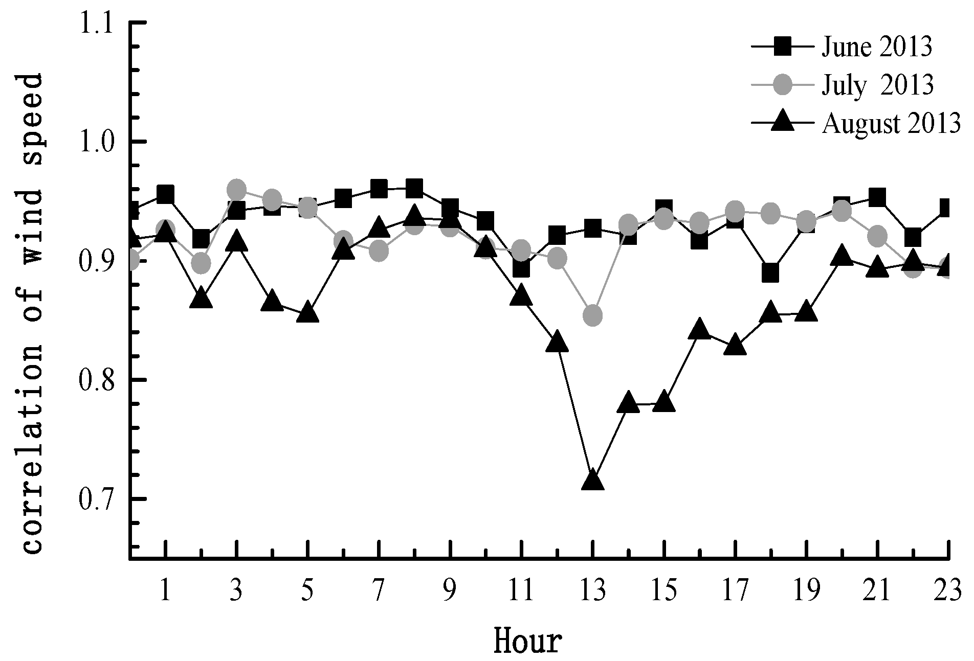
3.2.3. WSC at the Hourly Time Scale
This part mainly analyzes the correlation characteristics of the wind speeds in different periods of time of the day. The wind speed data of the target wind turbines during June through August 2013 are extracted for statistical calculation. The data are calculated on an hourly basis from midnight to 23:00. The results are shown in Figure 7.
As can be seen, for most parts of the day, the WSC coefficient between the two wind turbines stayed above 0.9, with a minimum of 0.7. That is to say, there was strong correlation between the wind speeds of the turbines. But between 11:00 and 13:00, the correlation decreased sharply.
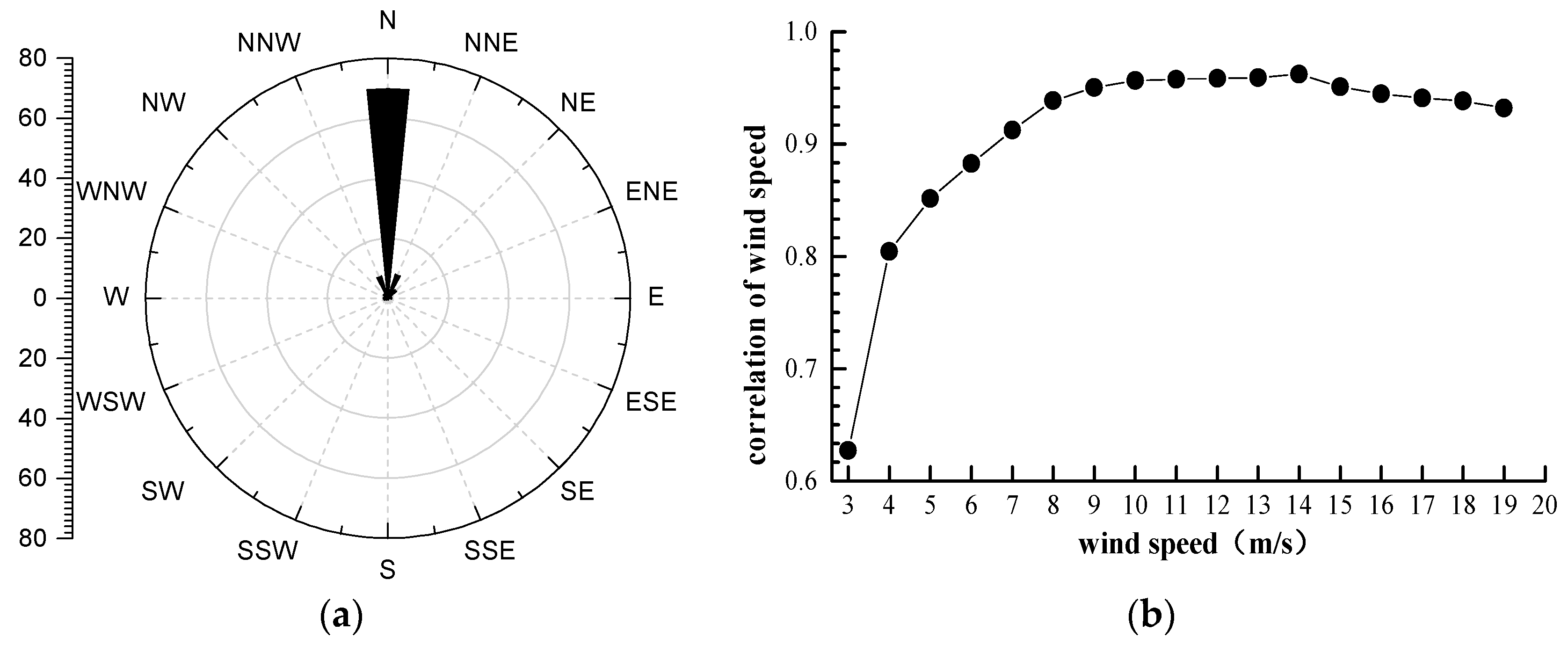
3.2.4. WSC of Different Wind Speed Ranges
Wind speed is a direct manifestation of the wind farm meteorological condition. In this part, the influence of wind speed magnitude on wind speed consistency between the wind turbines is analyzed. Calculations are performed based on the wind speed data in June 2013, which are grouped by the magnitude of wind speed, with an increment of 1 m/s. The results of correlation are shown in Figure 8b. In order to avoid the possible influence of the wind zones on WSC statistics, the wind rose of the month is drawn, as shown in Figure 8a. The wind was mainly in the north wind zone, and the wind direction had no obvious change.
The correlation coefficient shows a steady upward trend. In the case of a small wind speed, the correlation is low, with a minimum of 0.62, but the correlation coefficient increases with the wind speed. If the wind speed is relatively large, say, 8 m/s or beyond, the correlation becomes very strong and stable, reaching approximately 0.94. From this, it can be seen that the WSC between wind turbines is directly related to the magnitude of wind speed.
3.2.5. WSC of Different Wind Direction Zones
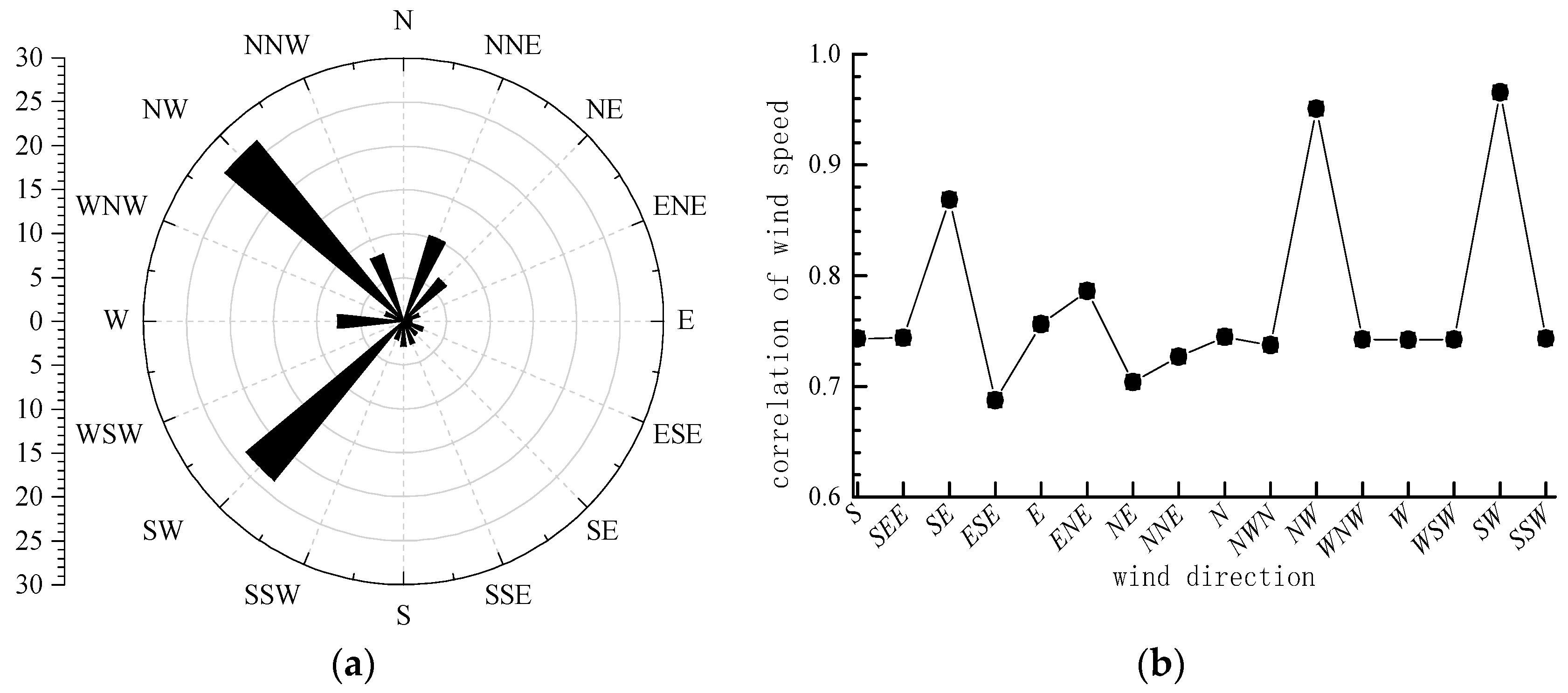
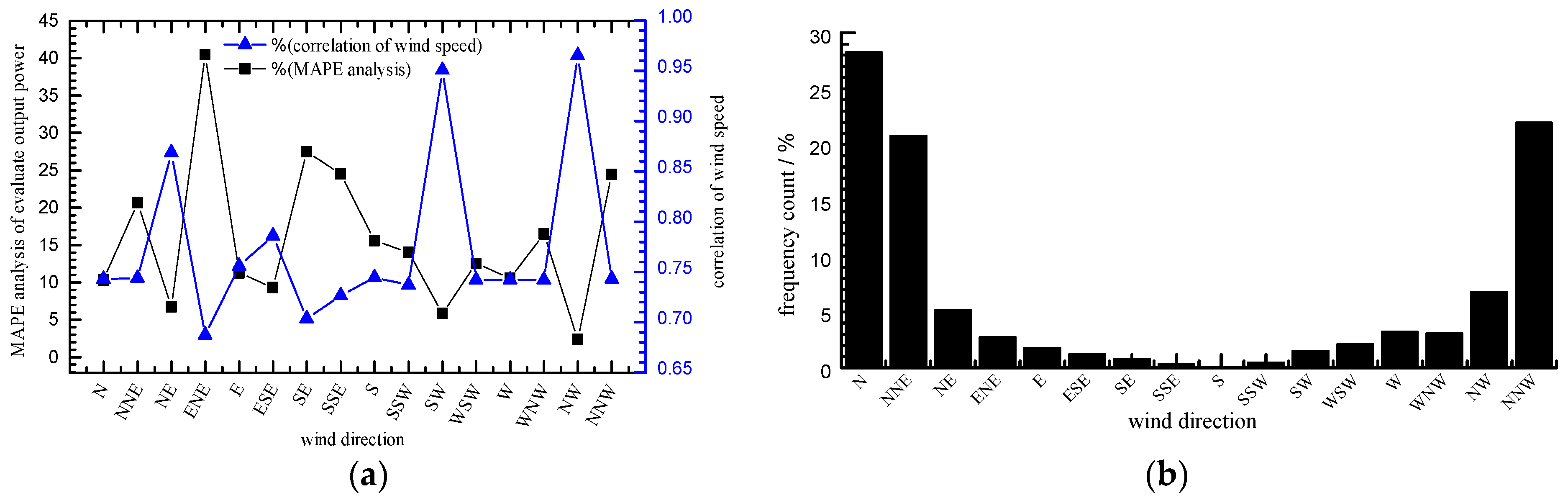
Wind speed and wind direction are closely meteorological related to each other, so it is necessary to analyze the impacts of wind direction on WSC. According to the wind direction division rules of the wind power industry, wind direction is divided into 16 zones, each being 22.5°. Analysis is made of the consistency correlation between wind turbines within each wind direction zone, and the results are given in Figure 9.
It is clear that the WSC in the southwest and northwest wind direction zones is significantly higher than that in other zones, with a correlation coefficient of up to 0.95 and a minimum of 0.65. Draw its wind roses of historical moments, and it is found that wind turbines are most widely distributed in the southwest and northwest wind direction zones. Therefore, the WSC of wind turbines is related to the wind direction zone and is most affected by the dominant wind direction.
4. Discussion and Outlook
The statistical analysis of time and meteorological WSC between wind turbines of a wind farm in Zhangbei wind power base suggests that the WSC has the following characteristics:
- The WSC shows an obvious seasonal trend. In Figure 5 of the case analysis part, the correlation coefficient between wind turbines decreased from 0.9 to 0.6 in the second half of the year and rose to 0.85 in the first half of the year;
- The WSC at the daily time scale shows dynamic fluctuations, and in some periods of the day it changes considerably. As presented in Figure 6, the correlation coefficient has a fluctuation of up to 0.3 on different dates of the month, and the correlation coefficient of two wind turbines can reach more than 0.3 on the same date in different months;
- The WSC between wind turbines is largely affected by wind speed and wind direction. As shown in Figure 7, for wind speeds of over 8 m/s, the correlation coefficient of wind turbines can be up to 0.94, and it might be as low as 0.7 for a low wind speed. In Figure 8, the southwest and northwest wind direction zones have an obviously higher WSC coefficient than other wind direction zones, reaching 0.95. For the dominant wind direction and medium-high wind speeds (8~18 m/s), wind turbines show strong consistency.
The seasonal variation, wind speed zone difference, and wind directionality contribute to the change of WSC between wind turbines. Different time periods, wind speeds and wind directions cause the correlation to vary. These factors, theoretically, affect the accuracy and reliability of wind farm equivalent modeling and wind power prediction based on WSC. In this paper, the T32 and T33 wind turbines have been used as an example for correlation equivalence and power prediction error check analysis.
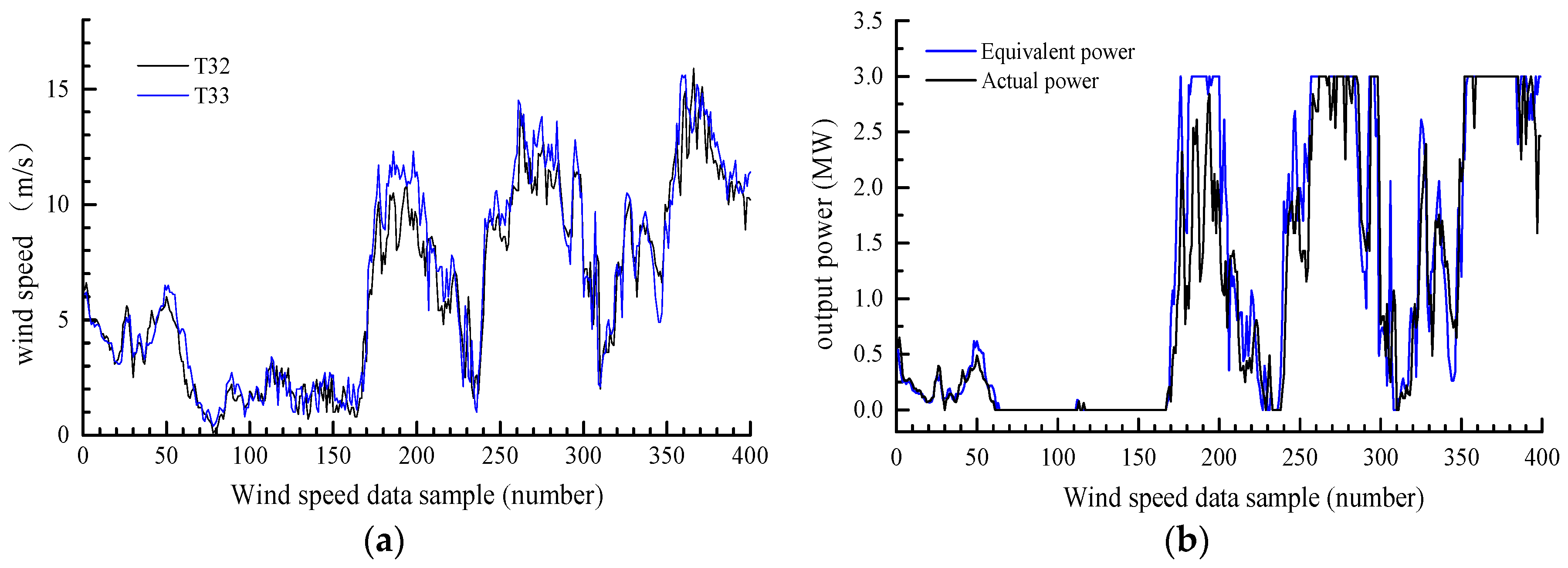
Shown in Figure 10 are the equivalent power curve and the actual power curve based on 400 sampling points from the operation data the two wind turbines in the case analysis. (The global WSC of the selected sampling points is 0.875, and therefore they are highly correlated.) The equivalent power curve is twice the power generation curve of T32, and it is used to simulate T32 and T33 in equivalent modeling simulation calculation. The actual power curve is the combined output power of T32 and T33 in simulated modeling.
It can be seen from Figure 9 that when the wind speed is too low to reach the cut-in speed, its output power is zero. The ultra-low wind speeds have been removed during the data cleaning stage, and has no effect on the output power equivalence of the wind turbines. When the wind speed value reaches the rated value or above, the correlation between the two turbines is high and stable. A comparison with the actual output power shows that both turbines are operating at the rated power. In theory, equivalent turbines are used for simplicity while achieving accuracy. For medium-high wind speeds, there is a rather big difference between the turbine’s equivalent output power and its actual power, with great fluctuations. In the strong WSC range, the error between the turbine’s equivalent power and actual power is small, and the error increases noticeably in the weak correlation range.
Figure 11 shows the output power equivalent error proportional distribution statistics of the two wind turbines in different wind speed ranges. It can be seen that the equivalent error of the output power at different wind speeds is approximately normal distribution. The higher the correlation between the wind turbines (higher wind speeds), the more concentrated the error distribution of the output power, and the smaller the error. When the WSC is high, the output power error is between 5~10%, while the error can reach 20~30% when the WSC is relatively weak (lower wind speeds).
Obviously, there are some limitations of wind turbines’ equivalent simplifying & modeling and wind power prediction based on the global WSC index. In some cases, equivalent wind turbines with strong global correlation might be in the low wind speed range or non-dominant wind direction zone, the equivalence and prediction errors caused by global calculation might be great. Therefore, it is necessary to study the influence of WSC on turbine equivalence and prediction accuracy by the time period, wind speed range and wind direction zone.
Based on the same turbines of T32 and T33 above, their historical operation data from June 2013 to February 2014 were analyzed, the time and meteorological WSC equivalence/prediction error analysis was carried out. The results are as follows.
• Analysis of the influence of WSC at different time scales
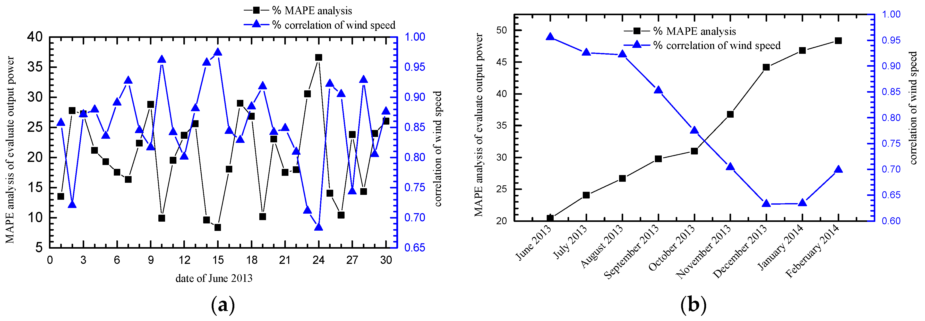
Figure 12 shows the equivalent power error curves of T32 and T33 from January 2013 to February 2014 at monthly and daily time scales, respectively.
It can be seen that there is a significant negative correlation between the WSC coefficient and the equivalent error. That is, the stronger the WSC between the turbines, the higher the equivalence accuracy. The error is less than 10%, which meets the modeling and power prediction requirements. When the WSC decreases to moderate correlation or below, the equivalent error will increase significantly to 20% or more, which is not suitable for equivalence reduction In addition, the seasonal characteristics of WSC also indicate that in turbine equivalence and power prediction we should distinguish the month and dynamic grouping equivalent in order to improve the equivalence accuracy.
• Analysis of the influence of WSC in different wind speed ranges
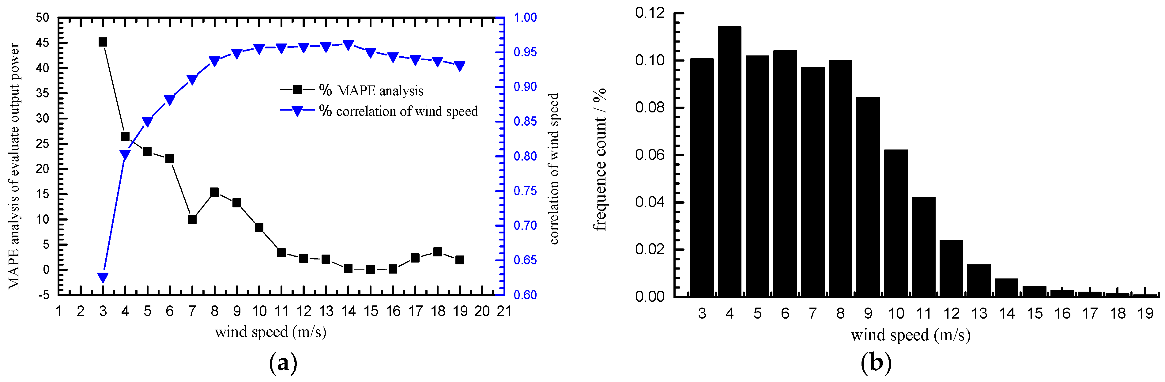
The error distribution of wind turbine equivalence in different wind speed ranges is shown in Figure 13. Apparently, in the medium and high wind speed ranges, the turbine equivalence accuracy and power prediction accuracy are both high, with an error of below 5%. However, the global equivalent error calculated by using the global WSC is 25%. To figure out why this happens, let us draw the wind speed-frequency histogram of the wind turbine.
It is obvious that the actual wind speed of the wind turbine is in Weibull distribution. The medium and low wind speeds account for more than 80%, resulting in a relatively large prediction error of global equivalence. The wind speed variability due to WSC directly affects the accuracy of turbine equivalence. The correlation test in different wind speed ranges and the dynamic grouping equivalence can reduce the error of equivalent prediction dramatically. Theoretically, the equivalent error can be reduced to 10%.
• Analysis of the influence of WSC in different wind direction zones
Figure 14 shows the equivalent error analysis of T32 and T33 in different wind direction zones, whose division is based on the international standard rule.
It can be seen that the wind turbine has good equivalence in some wind direction zones, with the power output error being less than 5%. But according to the wind rose, the wind direction zones with high WSC account for only 3% of the total. Its excellent equivalent effect is overwhelmed by most of the wind direction zones with poor equivalent effect, leading to the equivalent error calculated by using the global WSC being up to 25%. The equivalence of the wind turbine and its power prediction should be made with the directionality of the WSC in mind, and dynamic equivalent modeling should be carried out according to specific wind direction zones in order to make the equivalent modeling of wind farms more accurate and scientific.
In view of the time variability, wind speed difference, and directionality of the WSC between wind turbines, together with the multi-dimensional equivalent error analysis results, the author recommends the following basic strategies in wind farm equivalent modeling and wind speed/wind power prediction.
- For different follow-up applications of WSC, it is necessary to calculate the correlation between wind turbines under different dimensions.
- Wind turbines should be grouped dynamically according to the WSC coefficients at different time scales. While making wind speed/wind power predictions, we need to distinguish between low and high wind speeds, dominant and non-dominant wind directions.
5. Conclusions
The proposed data cleaning method for WSC can effectively eliminate dirty data and improve the data quality. And the proposed WSC calculation process is proved to be effective in correlation calculation for wind speed spatial, time and meteorological correlation between the wind turbines. The results of case study show that the time WSC is time-varying and displays significant differences for different seasons, time periods, wind speeds, and wind directions; The WSC is high and stable when the wind turbine is under the circumstance of dominant wind direction or middle/high wind speed; By contrast, the spatial WSC cannot illustrate these differences and variances, it has limitations. Differentiating the spatial, time, meteorological WSC can reduce the error of wind farm equivalent modeling and wind power forecasting. The quantitative analysis of the impacts of WSC between wind turbines under different time/meteorological conditions and strategies for coping with them are of great engineering value.
Author Contributions
Xiaojun Shen led the research scheme; Chongcheng Zhou performed the experiments; and analyzed the data; Chongcheng Zhou and Xuejiao Fu wrote and revised the paper.
Conflicts of Interest
The authors declare no conflicts of interest.
References
- Guo, Y.; Gao, H.; Wu, Q. A Combined Reliability Model of VSC-HVDC connected Offshore Wind Farms Considering Wind Speed Correlation. IEEE Trans. Sustain. Energy 2017, 8, 1637–1646. [Google Scholar] [CrossRef]
- Ding, Y.; Singh, C.; Goel, L.; Ostergaard, J.; Wang, P. Short-Term and Medium-Term Reliability Evaluation for Power Systems with High Penetration of Wind Power. IEEE Trans. Sustain. Energy 2014, 5, 896–906. [Google Scholar] [CrossRef]
- Yang, T.; Wang, J.; Song, S.S.; Liu, C.X. Dynamic Economic Dispatch of Power System Considering the Correlation of the Wind Speed. Trans. China Electrotech. Soc. 2016, 31, 189–197. [Google Scholar]
- Bechrakis, D.A.; Sparis, P.D. Correlation of wind speed between neighboring measuring stations. IEEE Trans. Energy Convers. 2004, 19, 400–406. [Google Scholar] [CrossRef]
- Peng, X.; Zheng, W.; Zhang, D.; Liu, Y.; Lu, D.; Lin, L. A novel probabilistic wind speed forecasting based on combination of the adaptive ensemble of on-line sequential ORELM (Outlier Robust Extreme Learning Machine) and TVMCF (time-varying mixture copula function). Energy Convers. Manag. 2017, 138, 587–602. [Google Scholar] [CrossRef]
- Ye, L.; Zhao, Y.; Zeng, C.; Zhang, C. Short-term wind power prediction based on spatial model. Renew. Energy 2017, 101, 1067–1074. [Google Scholar] [CrossRef]
- Qin, Z.; Li, W.; Xiong, X. Generation system reliability evaluation incorporating correlations of wind speeds with different distributions. IEEE Trans. Power Syst. 2013, 28, 551–558. [Google Scholar] [CrossRef]
- Chen, N.; Qian, Z.; Meng, X. Multi-step Ahead Speed Forecasting Model Based on Spatial Correlation and Support Vector Machine. Trans. China Electrotech. Soc. 2013, 28, 15–21. [Google Scholar]
- Chen, F.; Li, F.; Wei, Z.; Sun, G.; Li, J. Reliability models of wind farms considering wind speed correlation WSC and WTG outage. Electr. Power Syst. Res. 2015, 119, 385–392. [Google Scholar] [CrossRef]
- Xie, M.; Xiong, J.; Liu, M. Modeling of multi wind farm output correlation based on Copula and its application in power system economic dispatch. Power Syst. Technol. 2016, 40, 1100–1106. [Google Scholar]
- Zhou, Y.; Smith, S.J. Spatial and time patterns of global onshore wind speed distribution. Environ. Res. Lett. 2013, 8, 034029. [Google Scholar] [CrossRef]
- Salmon, J.R.; Walmsley, J.L. A two-site correlation model for wind speed, direction and energy estimates. J. Wind Eng. Ind. Aerodyn. 1999, 79, 233–268. [Google Scholar] [CrossRef]
- Li, Y.; Xie, K.; Hu, B. A Copula function-based dependent model for multivariate wind speed time series and its application in reliability assessment. Power Syst. Technol. 2013, 37, 840–846. [Google Scholar]
- Li, P.; Guan, X.; Wu, J.; Zhou, X. Modeling Dynamic Spatial Correlations of Geographically Distributed Wind Farms and Constructing Ellipsoidal Uncertainty Sets for Optimization-Based Generation Scheduling. IEEE Trans. Sustain. Energy 2015, 6, 1594–1605. [Google Scholar] [CrossRef]
- Damousis, I.G.; Alexiadis, M.C.; Theocharis, J.B.; Dokopoulos, P.S. A fuzzy model for wind speed prediction and power generation in wind parks using spatial correlation. IEEE Trans. Energy Convers. 2004, 19, 352–361. [Google Scholar] [CrossRef]
- Li, Y.; Li, W.; Yan, W.; Yu, J.; Zhao, X. Probabilistic optimal power flow considering correlations of wind speeds following different distributions. IEEE Trans. Power Syst. 2014, 29, 1847–1854. [Google Scholar] [CrossRef]
- Fan, R.; Chen, J.; Duan, X.; Li, H.; Yao, M. Impact of wind speed correlation on probabilistic load flow. Autom. Electr. Power Syst. 2011, 35, 18–22. [Google Scholar]
- Xie, K.; Billinton, R. Considering wind speed correlation of WECS in reliability evaluation using the time-shifting technique. Electr. Power Syst. Res. 2009, 79, 687–693. [Google Scholar] [CrossRef]
- Qin, Z.; Li, W.; Xiong, X. Reliability assessment of composite generation and transmission system considering wind speed correlation. Autom. Electr. Power Syst. 2013, 37, 47–52. [Google Scholar]
- Xue, Y.; Chen, N.; Wang, S.M.; Wen, F.S.; Lin, Z.Z.; Wang, Z. Review on Wind Speed Prediction Based on Spatial Correlation. Autom. Electr. Power Syst. 2017, 41, 161–169. [Google Scholar]
- Chen, N.; Xue, Y.; Ding, J.; Chen, Z.L.; Wang, X.Z.; Wang, N.B. Ultra-short Term Wind Speed Prediction Using Spatial Correlation. Autom. Electr. Power Syst. 2017, 41, 124–130. [Google Scholar]
- Zhang, S.M.; Dong, M.; Wang, B.Y. Application of Big Data Processing Technology in Fault Diagnosis and Early Warning of Wind Turbine Gearbox. Autom. Electr. Power Syst. 2016, 40, 129–134. [Google Scholar]
- Li, C.; Shen, Z.; Meng, K.F.; Yin, S.; Yan, M. Filter Method of Fitting Data of Wind Turbine Power Curve based on Skewness Index. In Proceedings of the 2013 China Electrical Engineering Society Annual Meeting, Chengdu, China, 21 November 2013; pp. 1–5. [Google Scholar]
- Chang, T.P.; Liu, F.J.; Ko, H.H.; Huang, M.C. Oscillation characteristic study of wind speed, global solar radiation and air temperature using wavelet analysis. Appl. Energy 2017, 190, 650–657. [Google Scholar] [CrossRef]
- Lin, Q.; Wang, J. Vertically Correlated Echelon Model for the Interpolation of Missing Wind Speed Data. IEEE Trans. Sustain. Energy 2014, 5, 804–812. [Google Scholar] [CrossRef]
- Sun, C.; Bie, Z.; Xie, M.; Jiang, J. Fuzzy Copula model for wind speed correlation and its application in wind curtailment evaluation. Renew. Energy 2016, 93, 68–76. [Google Scholar] [CrossRef]
Figure 1.
Flow diagram of wind speed operation data cleaning and sorting.
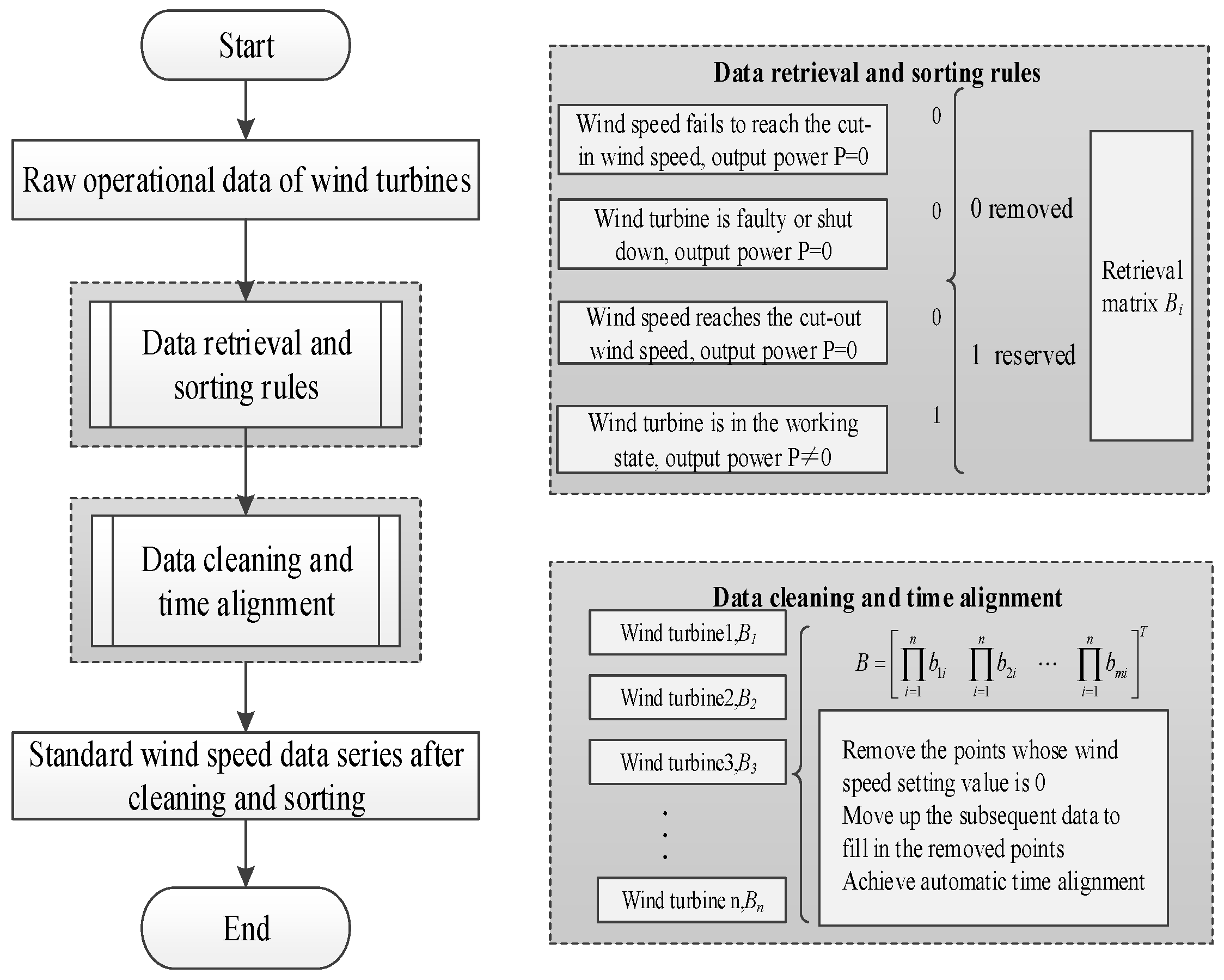
Figure 2.
Diagram of wind speed sampling period selection rule.

Figure 3.
Calculation flow of wind speed correlation.
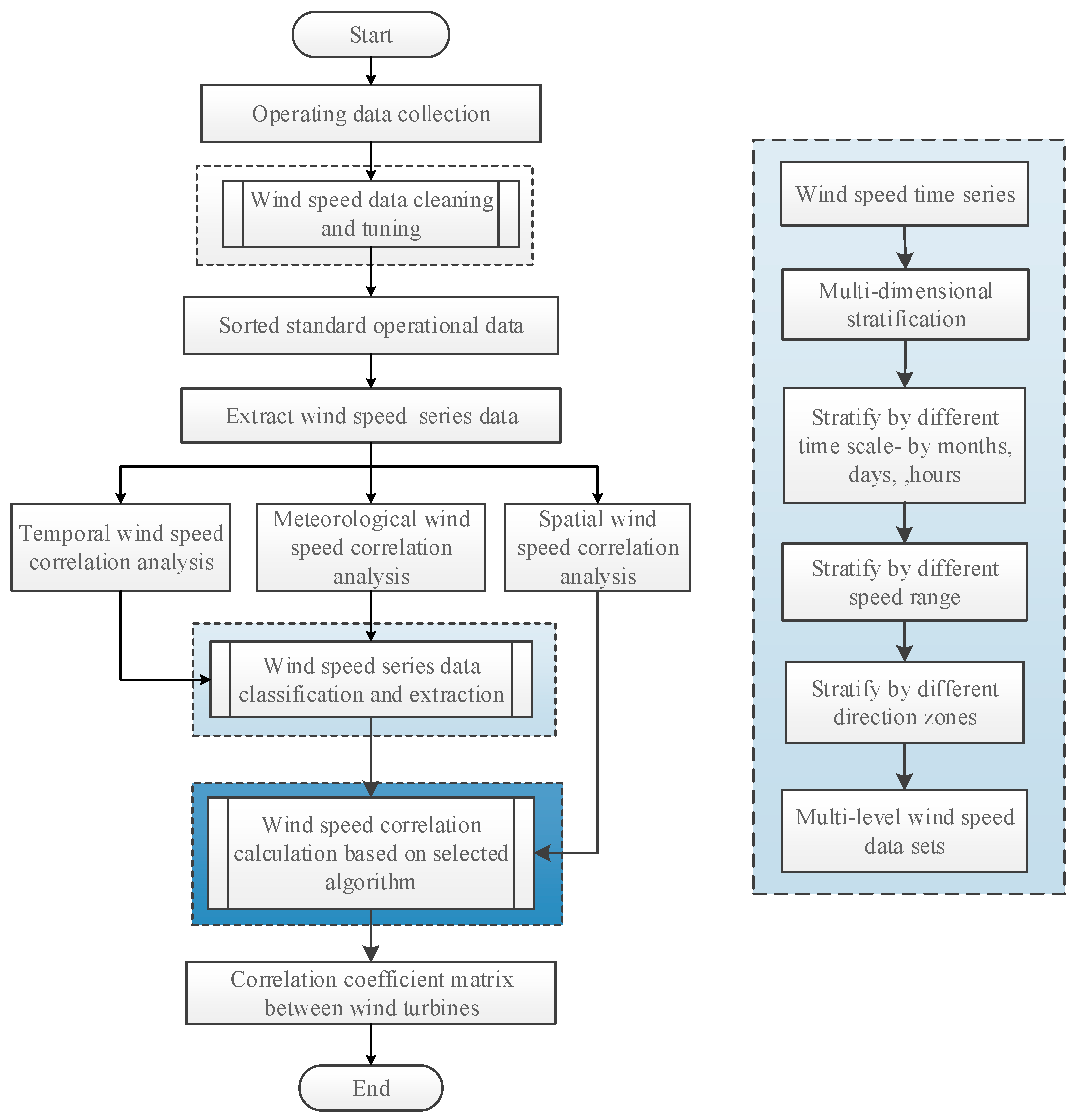
Figure 4.
Original wind speed data and cleaned wind speed data; (a) original data; (b) cleaned and sorted data.
Figure 4.
Original wind speed data and cleaned wind speed data; (a) original data; (b) cleaned and sorted data.
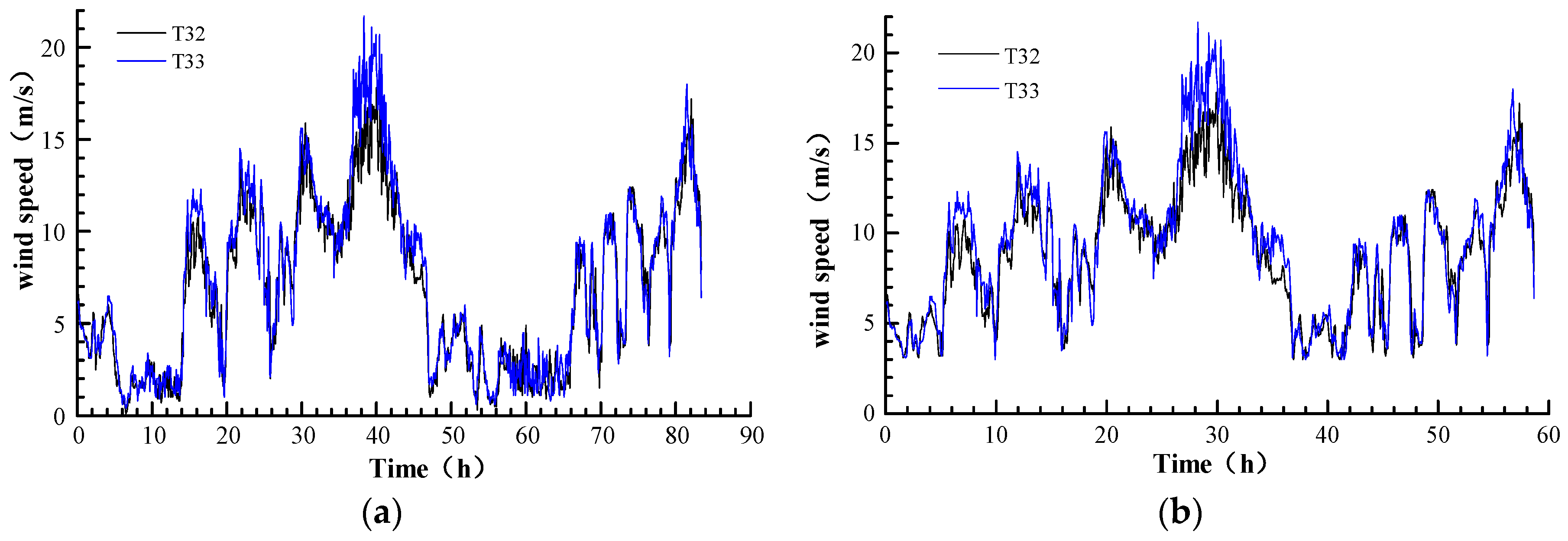
Figure 5.
Statistical curve of WSC coefficient in different month.

Figure 6.
Statistical curve of WSC coefficient in different day.

Figure 7.
Statistical curve of WSC coefficient in different hours.

Figure 8.
Statistical curve of WSC coefficient under different wind speed segment; (a) Wind rose; (b) Statistical curve of WSC coefficient under different wind speed segment.
Figure 8.
Statistical curve of WSC coefficient under different wind speed segment; (a) Wind rose; (b) Statistical curve of WSC coefficient under different wind speed segment.

Figure 9.
Statistical curve of WSC coefficient under different wind directions zone; (a) Wind rose; (b) Statistical curve of WSC coefficient under different wind directions zones.
Figure 9.
Statistical curve of WSC coefficient under different wind directions zone; (a) Wind rose; (b) Statistical curve of WSC coefficient under different wind directions zones.

Figure 10.
Comparison curve of equivalent power and actual power; (a) Actual wind speed curves; (b) Equivalent power curve and actual power curve.
Figure 10.
Comparison curve of equivalent power and actual power; (a) Actual wind speed curves; (b) Equivalent power curve and actual power curve.

Figure 11.
Error distribution of output power under different wind speed.

Figure 12.
WSC coefficient and equivalent power error at different time scales; (a) Equivalent error at daily time scale; (b) Equivalent error at monthly time scale.
Figure 12.
WSC coefficient and equivalent power error at different time scales; (a) Equivalent error at daily time scale; (b) Equivalent error at monthly time scale.

Figure 13.
Equivalent error distribution in different wind speed ranges; (a) Equivalent error in different wind speed ranges; (b) Wind speed-frequency histogram.
Figure 13.
Equivalent error distribution in different wind speed ranges; (a) Equivalent error in different wind speed ranges; (b) Wind speed-frequency histogram.

Figure 14.
Equivalent error distribution in different wind direction zones; (a) Equivalent error in different wind direction zones; (b) Wind speed-frequency histogram.
Figure 14.
Equivalent error distribution in different wind direction zones; (a) Equivalent error in different wind direction zones; (b) Wind speed-frequency histogram.

© 2018 by the authors. Licensee MDPI, Basel, Switzerland. This article is an open access article distributed under the terms and conditions of the Creative Commons Attribution (CC BY) license (http://creativecommons.org/licenses/by/4.0/).
Share and Cite
MDPI and ACS Style
Shen, X.; Zhou, C.; Fu, X. Study of Time and Meteorological Characteristics of Wind Speed Correlation in Flat Terrains Based on Operation Data. Energies 2018, 11, 219. https://doi.org/10.3390/en11010219
AMA Style
Shen X, Zhou C, Fu X. Study of Time and Meteorological Characteristics of Wind Speed Correlation in Flat Terrains Based on Operation Data. Energies. 2018; 11(1):219. https://doi.org/10.3390/en11010219
Chicago/Turabian StyleShen, Xiaojun, Chongcheng Zhou, and Xuejiao Fu. 2018. "Study of Time and Meteorological Characteristics of Wind Speed Correlation in Flat Terrains Based on Operation Data" Energies 11, no. 1: 219. https://doi.org/10.3390/en11010219
Note that from the first issue of 2016, this journal uses article numbers instead of page numbers. See further details here.