Modeling the Risk of Commercial Failure for Hydraulic Fracturing Projects Due to Reservoir Heterogeneity


1
School of Science, Engineering and Design, Teesside University, Middleborough TS1 3BA, UK
2
Department of Petroleum Engineering, Petroleum, Gas and Petrochemical Faculty, Persian Gulf University, Bushehr 75169-13817, Iran
*
Author to whom correspondence should be addressed.
Energies 2018, 11(1), 218; https://doi.org/10.3390/en11010218
Submission received: 16 November 2017
/
Revised: 23 December 2017
/
Accepted: 12 January 2018
/
Published: 17 January 2018
(This article belongs to the Section L: Energy Sources)
Abstract
:Hydraulic fracturing technologies play a major role in the global energy supply and affect oil pricing. The current oil price fluctuations within 40 to 55 USD per barrel have caused diminished economical margins for hydraulic fracturing projects. Hence, successful decision making the for execution of hydraulic fracturing projects requires a higher level of integration of technical, commercial, and uncertainty analyses. However, the complexity of hydraulic fracturing modeling, and the sensitivity and the effects of uncertainty of reservoir heterogeneity on well performance renders the integration of such studies rather impractical. The impact of reservoir heterogeneity on hydraulic fracturing performance has been quantified by the introduction of Heterogeneity Impact Factor (HIF) and formulas have been developed to forecast well performance using HIF. These advances provide a platform for introducing a practical approach for introducing the Risk of Commercial Failure (RCF) due to reservoir heterogeneity in hydraulic fracturing projects. This paper defines such a parameter and the methodology to calculate it in a time-efficient manner. The proposed approach has been exercised on a real project in which a RCF of 20% is computed. The analysis also covers the sensitivity on Capital Expenditure (CAPEX), Operational Expenditure (OPEX), gas price, HIF and discount rate.
1. Introduction
The high energy prices from 2007 to 2014 led to the exploitation of more hydrocarbons from oil and gas reservoirs around the globe. However, with the production decline of conventional reserves, the petroleum industry has shifted more towards the development and production of unconventional hydrocarbon resources. In this sense, improving gas recovery from unconventional gas resources such as shale gas [1,2,3,4] and tight gas [5,6,7] reservoirs using the hydraulic fracturing technology has proved to be effective in supplying a part of the increasing global energy demand. Some examples of hydraulic fracturing applications have been reported all around the world [8,9,10,11,12]. Although the fracturing technique is now considered an essential part of the reservoir management backbone in tight/shale gas field developments, the complexities associated with the hydraulic fracturing dictate some degree of uncertainty in successful economic applications [6,13,14,15,16]. Some prominent characteristics of these reservoirs, such as very low permeability and high initial gas flow rate followed by a sharp decline, cause the economic evaluation of the process to be usually accompanied with significant difficulties. Quantification and understanding the associated risk and uncertainty provides grounds for determining whether a particular hydraulic fracturing job can be commercially feasible or not [17,18,19,20].
The chance of achieving commercial production is the main uncertainty in development of unconventional play. In this regard, Harding argued that a deterministic solution cannot account for the uncertainty of input assumptions. He presented a stochastic approach to evaluate several commercial realizations in which the risk of failure and uncertainty of success for different stages of the process was calculated [21]. There have also been suggestions on a stochastic approach based on multi-disciplinary participation and iterative modeling in unconventional project evaluation [22]. Williams-Kovacs and Clarkson developed tools that incorporate pre-drill screening, exploration, pilot, and commercial demonstration to quantify the risk and uncertainty in shale gas prospecting and development. This method employs production data analysis and forecasting approaches to compare shale gas prospects in a stochastic manner [23].
More recently, Liang et al. proposed a workflow in which an in-house uncertainty quantification package is jointed to hydraulic fracturing modeling and reservoir simulation. In this process, several parameters including permeability of the matrix, completion information, and fracture properties were incorporated. The proposed methodology utilized a top-down concept and can proceed the model from a big 3D model to pad-scale and single well models. This integrated approached has been applied to an unconventional reservoir factory-model development in the Permian Basin [24].
As can be inferred from the literature, despite the considerable number of fracking projects applied, relatively limited approaches are available in modeling and quantifying uncertainty and risk in successful application of massive hydraulic fracturing techniques. However, numerous investigations on uncertainty/risk analysis and optimization in reservoir simulation jobs have been reported. Therefore, from the decision-making point of view, a logical way to evaluate an unconventional asset can be achieved through incorporation of some characteristic features into these models. Among different approaches in this area, Thiele and Batycky have recently introduced a new methodology, called EVOLVE, to quantify the reservoir uncertainty [25]. This linear workflow is comprised of four key stages from screening and model selection to Net Present Value (NPV) calculation. Their work got use of streamline class of simulators, since streamline simulators have unique feature of capturing injector-producer connectivity [26,27,28]. As a main characteristic, EVOLVE deploys a distance-based generalizes sensitivity. They claim that this is a unique and powerful workflow that covers different aspects from geological and simulation parameters and forecast scenarios to economic evaluation [25]. Although this approach and the others which fall in such a category can result in a detailed characterization of different aspects of the reservoir, they would be extremely tedious and time consuming in case of heterogeneous reservoirs. There are other parameters that can be potentially incorporated into the sensitivity workflow, such as impact of geomechanically induced heterogeneity (porosity, permeability, and Net to Gross; NTG) in the reservoir either analytically [29] or numerically on reservoir scale [26]. Since heterogeneity is one of the main concerns in evaluating a hydraulic fracturing job in an unconventional gas reservoir, seeking a new quick method to account for the heterogeneity impact seems inevitable.
In this paper, following our previously-suggested formulas [30] for production forecasting of multi-fractured horizontal wells in heterogeneous tight gas reservoir (the main focus of this study), a highly time-efficient workflow is proposed from which the Risk of Commercial Failure (RCF) due to the impact of reservoir heterogeneity can be evaluated. To achieve this, our suggested gas flow model (decline curve using heterogeneity impact factor, DCH) was incorporated in an economic evaluation platform from which NPV of a hydraulic fracturing job could be calculated for a range of realizations. The sensitivity analysis included the reservoir heterogeneity in terms of Heterogeneity Impact Factor (HIF) as the main influencing parameter. In addition, the sensitivity of the other parameters such as Capital Expenditure (CAPEX), Operational Expenditure (OPEX), gas price, and discount rate to NPV was also reported. The output of the proposed approach was the computation of RCF.
2. Theoretical Background
2.1. Heterogeniety Impact Factor Determination
The hydraulic fracturing modeling can be linked to well test interpretation to quantify the effect of reservoir heterogeneity on the hydraulic fracture performance. In this sense, the HIF parameter was introduced in our previous works [30,31] to account for the degree of the connectivity of fracked wells to more permeable rocks or natural fractures. To define HIF, first, a measurable parameter called Surface Conductivity (SC) was defined, using facture properties, as:
where xf is the hydraulic fracture half length, hf is the fracture height, Kf is the fracture permeability, and w is the fracture width.
The state of art in definition of SC is the integration of all fracture properties in a single parameter. SC can be calculated for both well test analysis (WTA) and net pressure match (NPM) represented by SCWTA and SCNPM, respectively. HIF is then defined as the ratio of WTA and NPM surface conductivities:
This ratio is then used to adjust the fracture conductivity in the dynamic simulation model. HIF is related to the results of the observed data where both the production period and the aerial extent of reservoir properties are considered to compare with the performance expected from the fracking job. An HIF value of unity (or 100%) means that the well behaves as it has been modelled. HIF values greater than 1 show that the well outperforms the model, and HIF values less than 1 are indicative of under-performance of the well compared to the model.
2.2. Cumulative Gas Production Calculation
The gas production from a hydraulically fractured well in a heterogeneous reservoir can be calculated from the following empirical DCH model [30]:
where is the gas flow rate of well in a heterogeneous reservoir, is the production time, is the decline exponent, and are the initial rate and decline constant modified to account for HIF, respectively. The unit of is the reciprocal of time. Based on the history match analysis in our previous work [30], the initial production rate, and the decline constant, were suggested to be corrected for HIF using the following rules:
- (1)
- for HIF < 1: and
- (2)
- for HIF > 1: and
To calculate the produced cumulative gas from a well, Equation (3) should be integrated from the start of production to a specified time:
Evaluating the integral from zero to a time gives the following expression for cumulative gas production:
where must be in 1/day unit.
2.3. Economic Evaluation
There are different profitability indicators to evaluate the feasibility of a project from the economic standpoint. Here, the future production of a fractured well was economically evaluated through NPV calculation. NPV criterion is a robust economic evaluation tool and has been widely used in different petroleum industry projects [31,32,33]. The initial stage of NPV evaluation is to determine the proper parameters that encompass the objectivity of the whole process. In this way, the cash flow associated with the produced gas was calculated on the basis of expected CAPEX/OPEX and considering the economic variables such as gas price, discount rate, etc. The produced hydrocarbon selling price, CAPEX and discount rate were supposed to be the most important parameters in any gas development project. For a given CAPEX, required for drilling and stimulating a well, an income (or a revenue stream) of from gas selling was expected from which the following expression can be written for NPV calculation:
where i is the discount rate, OPEX is the annual operative expenditures, and is the years of production for which the process should be assessed. The annual revenue is obtained by:
where is the gas price and is the annual cumulative produced gas. was calculated from Equation (5) based on the difference of gas production values from time to .
2.4. Definition of Risk Due to Heterogeneity
We propose a definition of commercial failure due to reservoir heterogeneity as the probability of having NPV = 0 considering the uncertainty of HIF. To achieve this, a uniform distribution in lack of a large data set for the heterogeneity parameter was suggested. This can be tuned based on observations of off-set well production behaviour.
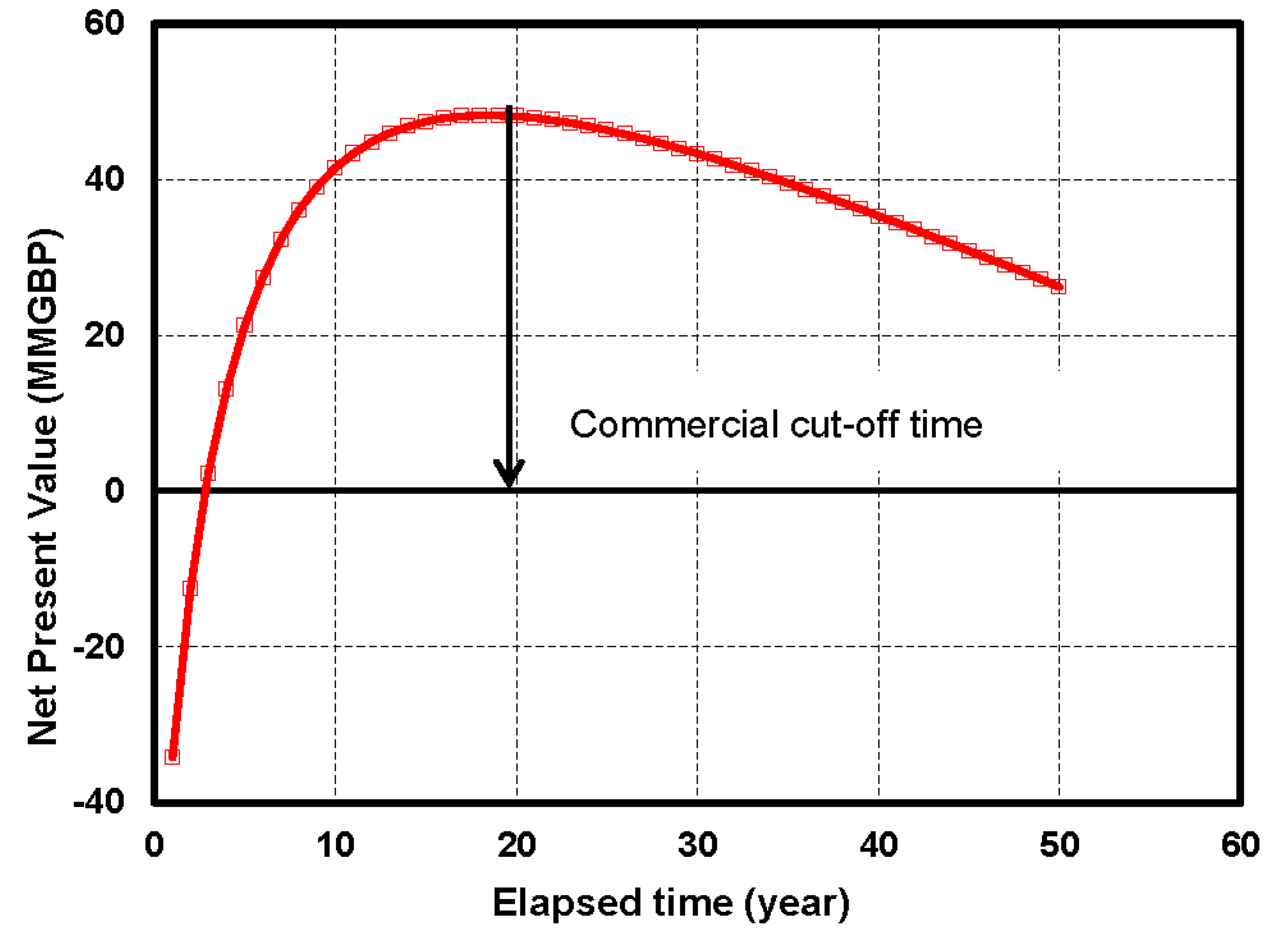
Given the appropriate values for CAPEX, OPEX, discount rate, and years of production, the NPV for a specified degree of heterogeneity was calculated on the annual basis. Having constructed the plot of NPV versus time for each value of HIF, the commercial cut off or operational stopping point was selected to be the maximum NPV. This process is schematically shown in Figure 1 which has been generated using the procedure described below:
- (1)
- Set a value for HIF; i.e., for any HIF an individual NPV history is achieved.
- (2)
- Calculate the modified flow rate and the decline constant considering the set HIF value.
- (3)
- Quantify the annual cumulative gas production from Equation (5) based on the difference of gas production values from to successive time intervals of n and n + 1.
- (4)
- Multiply the value obtained in step 3 by the gas price to calculate the annual revenue.
- (5)
- Discount the annual revenue for OPEX and discount rate on an annual base.
- (6)
- Subtract the discounted income resulted in step 6 from CAPEX.
- (7)
- Repeat the above steps for subsequent years of production and construct the NPV versus time plot.
Finally, the cumulative distribution plot for NPV (maximum over production time) was generated and the RCF for a hydraulic fracturing project was read from the value of zero for NPV.
3. Results and Discussion
3.1. Economical Model
In this section, the results of the economical modelling including sensitivity analysis for uncertain parameters are reported.
3.1.1. Assumption of Model Variables
Heterogeneity Impact Factor (HIF)
To have a reasonable corresponding range for HIF, we refer to our recent investigation [34] in which the impact of heterogeneity on hydraulic fracturing performance was discussed. In this regard, the HIF determination framework discussed in Section 2.1 was applied for available real field information from fracked wells drilled in a Southern North Sea reservoir. The obtained values for HIF were in the range of 0.35 to 1.73. Therefore, this interval was selected for NPV calculation in the following sections.
Cost and Income Issues
The capital and operating expenditures, gas price and discount rate are four main parameters in determining the profitability of a hydraulic fracturing job. The CAPEX is mainly the cost of the well construction (including drilling and completion activities), fracking fluids preparation, pipe line and pumping facilities, and proppants. Whether a well was drilled from an offshore platform or not affects the CAPEX to a significant extent. Based on recent commercial activities in North Sea [35], a representative range for CAPEX was selected to be 30–60 MMGBP with mid value of 45 MMGBP. In addition, a fraction of annual income must be consumed as OPEX (1–4 MMGBP per year). As another effective parameter, the gas price depends on different factors such as global/local demands and types and/or issues of contracts. It can be interrelated to the crude oil prices and changes with the increase/decrease in global oil price. However, the situation of no relation between oil and gas price was also encountered. Although the prediction of gas price is complicated, the economic evaluation of hydraulic fracturing is linked to cash flow resulted from the selling price of the produced gas. Therefore, one must estimate the price upper and lower bound to account for the commercial risk to some extent. Different gas prices reported for North Sea in recent years imply that a range of 4–6 GBP per MMSCF can be considered. The discount rate reveals the decrease in the value of future income. Some aspects such as the inflation and interest rate were taken into account by this parameter. For our case, in an optimistic low risk condition for investments, the discount rate was supposed to be 0.05. In the high risk environment, this value was allowed to be raised up to 0.15. Table 1 summarizes the uncertainty ranges for the economic parameters discussed above.
3.1.2. Sensitivity Analysis
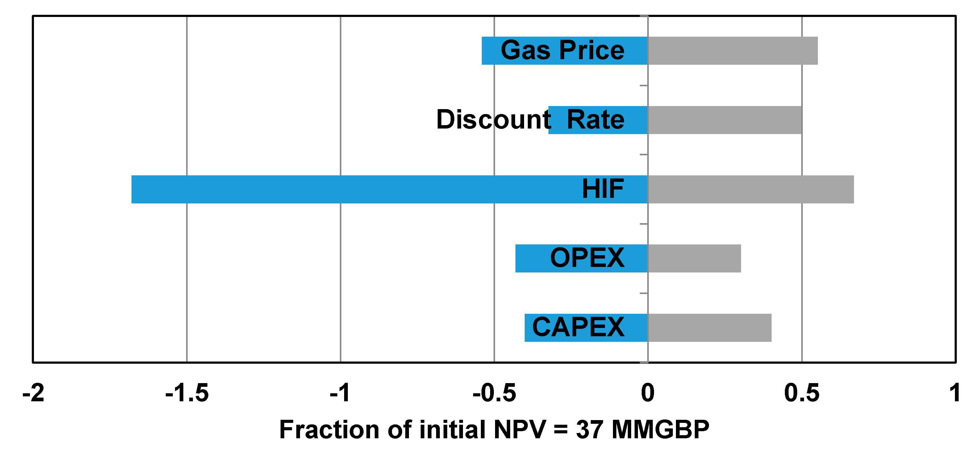
As discussed earlier, the values of economic parameters were subject to a degree of uncertainty in a reasonably pre-specified domain. Therefore, the dependence of the model response, i.e., NPV, on change in parameter values should be clarified. In this regard, a sensitivity analysis stage was performed through so called one-at-a-time approach. A given parameter was set to its lower and upper bound values when the rest of variables took their midpoint or base values. The results were emerged as a famous tornado chart. The related plots are shown in Figure 2 in which the effect of the four discussed economic variables as well as the heterogeneity impact (HIF) was explored. To better understand the significance of each parameter, the change in maximum NPV was normalized according to the base NPV value (considering the mid values for parameters). Indeed, the reported NPV in Figure 2 shows the fraction of increase/decrease in initial NPV due to change in a given parameter.
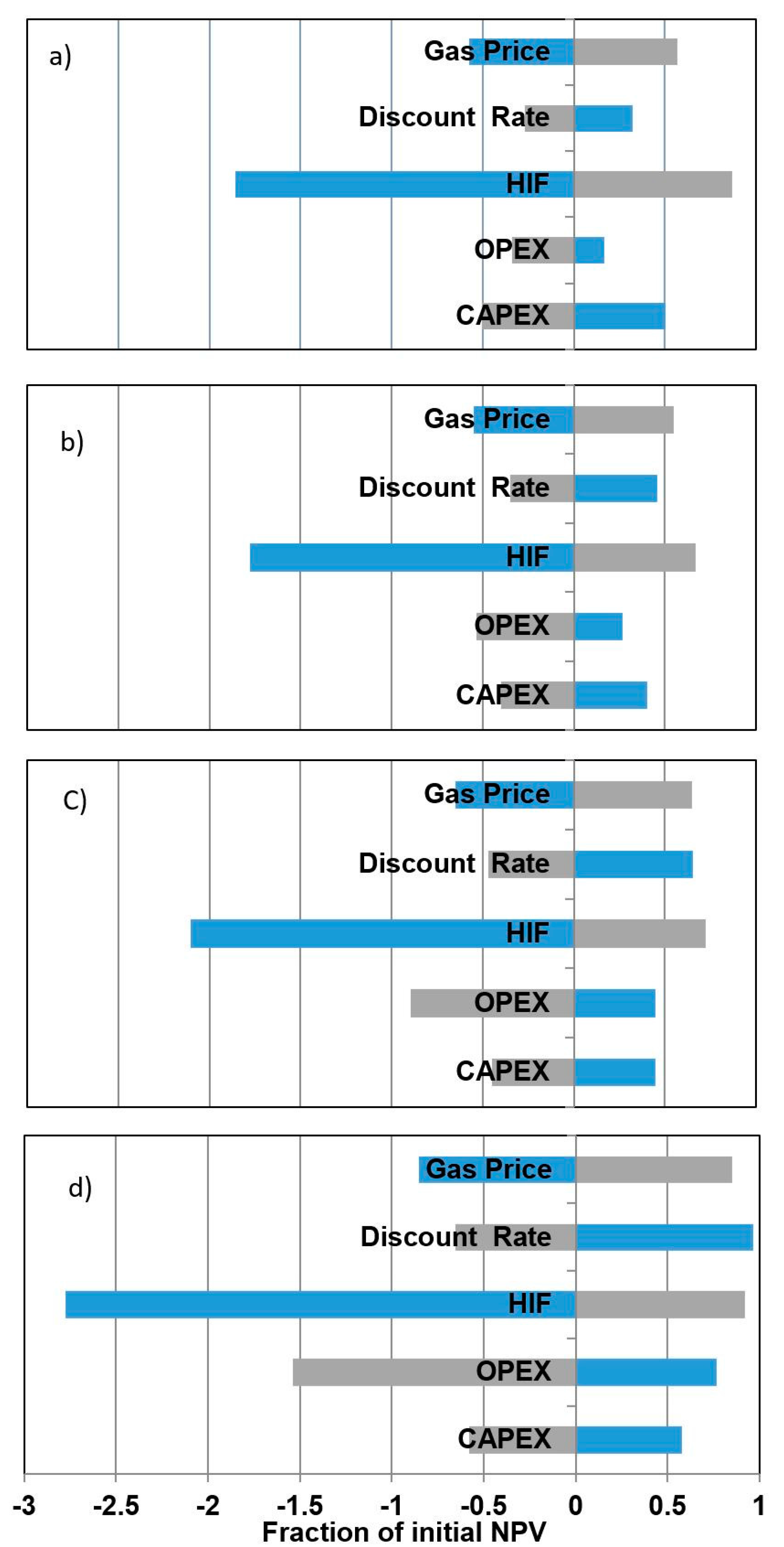
Although the whole project should be evaluated based on the maximum NPV, tracking the NPV history (i.e., the change in NPV over the production life of a given well) could lead to valuable insight into the individual role of contributing parameters. To achieve this goal, the sensitivity of NPV on different parameters was illustrated at the end of the 5th, 10th, 15th, and 20th years of production. Since the CAPEX is a constant cost paid at the initial stage of project, the variation of NPV due to the change in CAPEX did not depend on the time, and the tornado chart, in this case, showed approximately no variation.
The minor change in CAPEX around ±0.5 was due to change in the base NPV at the end of each specified time interval. The OPEX and discount rate were defined on an annual basis and so they did affect the NPV over time. Gas price was not assumed a time dependent variable but it impressed the NPV history due to increase in the cash flow related. The tremendous impact of HIF on the NPV change with time was undeniable but the situation was more remarkable as the HIF was not a transient variable. Dealing with the positive effect of parameters on NPV, one could find that the effects of different parameters tend to be somehow comparable. However, the negative effect was more pronounced in the case of HIF. Strictly speaking, the HIF was a time-independent parameter that influenced the profitability of the hydraulic fracturing project during the whole life time of the well/reservoir. The evaluation also demonstrated the significant role of heterogeneity on maximum NPV.
3.2. Single Field Case Study
3.2.1. Field Description
Babbage Field was discovered 80 km offshore off the UK in the North Sea by drilling the 48/2-2 well in 1988. The well flowed at a rate of 3.8 MMscf/d and was considered uneconomical for development for 18 years. A second well, 48/2a-4, was drilled onto the crest of the structure in 2006 which achieved a flow rate of 11 MMscf/d on test, establishing the presence of a significant gas accumulation. The geological history of the field has resulted in an illitised sandstone pay zone with a low permeability of about 0.1 mD and occasional higher permeability streaks (1 inch of 200 mD streaks observed on the core) and limited natural fractures. Such a wide range of permeability (from the reservoir rock tight matrix to high permeability streaks and the natural fracture system) explains the highly heterogenous nature of this field. This heterogeneity is reflected in the HIF analysis as an attempt to simplify the physics and quantify the heterogeneity impact on hydraulic fracturing. An HIF value of 1 represents the base tight formation with no better or worse properties. HIF < 1 indicates a more severe level of rock quality downgrade such as illitisation. HIF > 1 demonstrates the impact of high permeability streaks and/or natural fracture contributions. These approaches are already validated by well test and net-pressure matches of the fracs and references are provided. The calculated range of HIF 0.35 to 1.73 demonstrates how severe heterogeneity impact is on this field.
Since the illitisation has deteriorated the permeability of the field, the development required the hydraulic fracturing to make the project economically feasible. Babbage has undergone two phases of development well drilling to date. In Phase 1, between 2008 and 2010, three horizontal, multi-fracked wells (B1, B2z and B3) were drilled and successfully stimulated. First gas was achieved in August 2010. Phase 2 comprised the drilling of two horizontal, multi-fracked wells (B4 and B5y) from the platform in 2012–2013, with resultant first gas in October 2013 [35].
3.2.2. Modelling
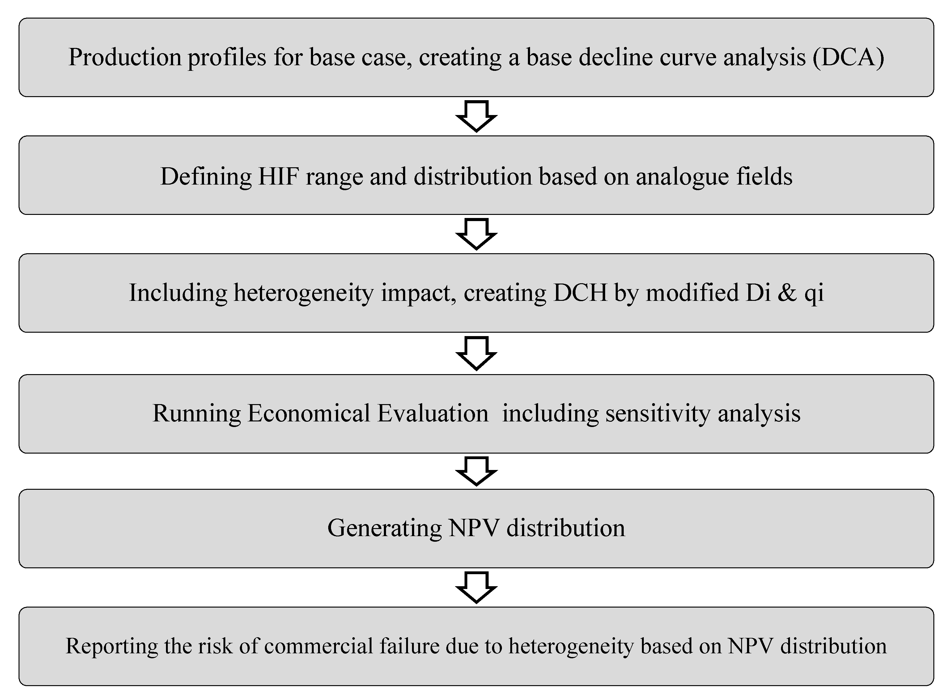
To model the RCF associated with a hydraulic fracturing project considering the heterogeneity of the gas reservoir, the workflow presented in Figure 4 was followed.
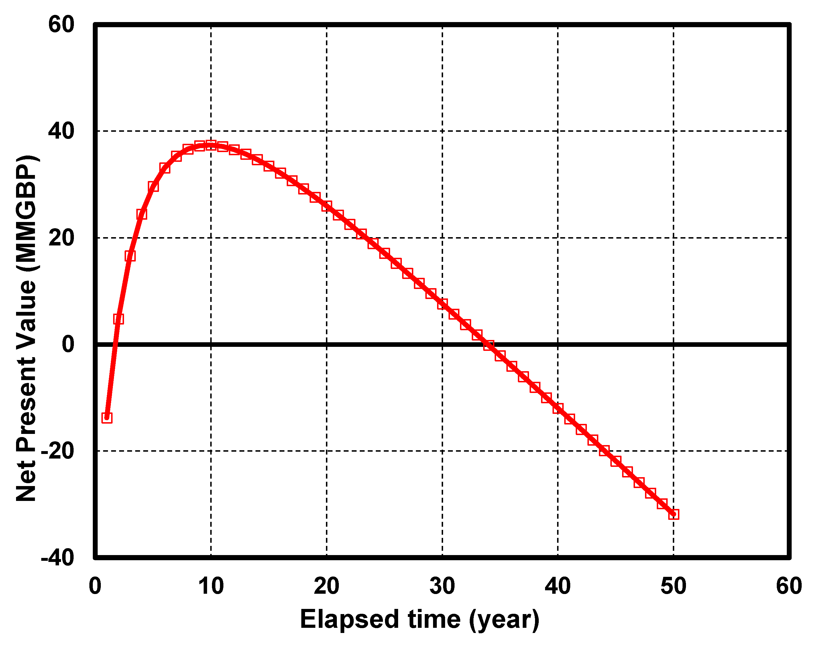
Using Babbage data, and observed range of HIF from 0.35 to 1.75 for Babbage wells, the model has been set up for 100 realisations of uniform HIF distribution with mid value assumptions of Table 1. The NPV versus time for each scenario has been calculated. Figure 5 demonstrates NPV versus time for the base case. This figure clearly demonstrates the very positive value of the project by year 10 which is the commercial cut-off for this scenario.
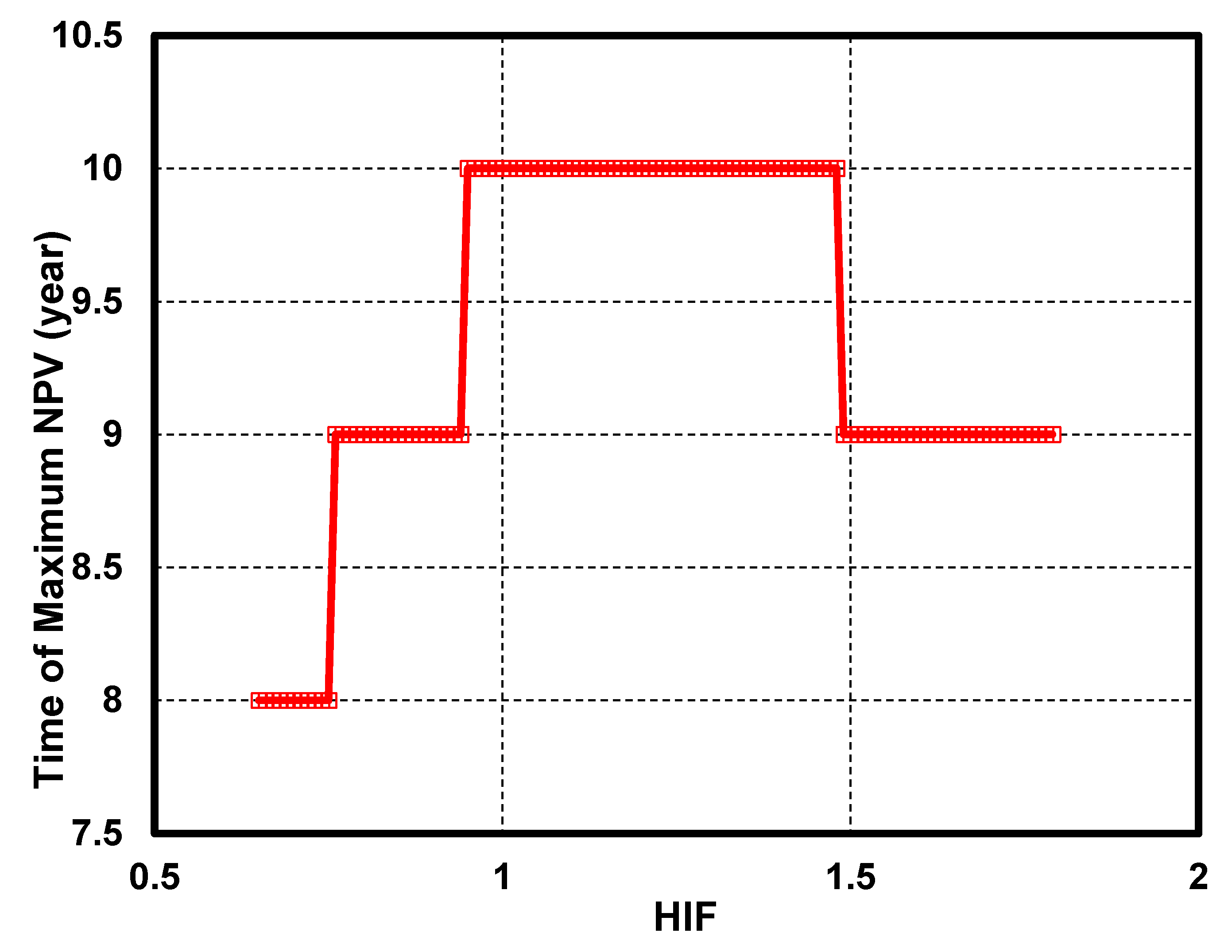
The commercial cut-off of each realization was calculated and reported for positive NPVs (8 to 10 years) versus HIF (Figure 6).
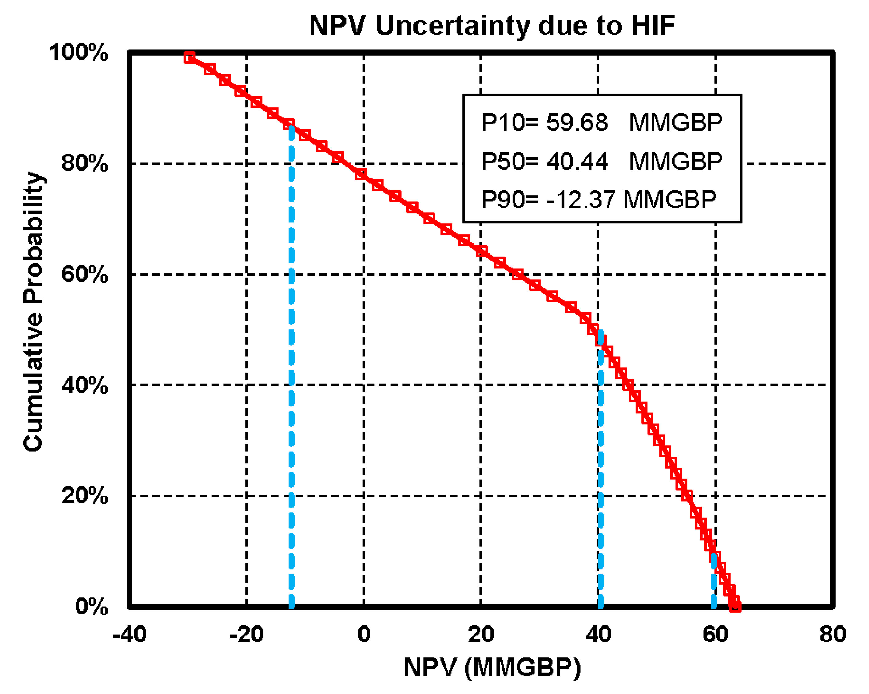
Finally, the cumulative probability of NPV was calculated using 100 realisations and P10, P50, P90 were reported as 60, 40 and −12 million GBP (Figure 7). The proposed term for the risk of commercial failure for this hydraulic fracturing project due to heterogeneity is 1 min the intersection of NPV = 0 and the cumulative NPV probability, i.e., 20%.
3.3. Validation
To evaluate the validity of RCF for a real case, we refer to the Babbage field. As discussed before, the field has five multi-fracked horizontal production wells. The NPV per well has been calculated to demonstrate any commercial failure of well development due to heterogeneity which is the only differentiator in this case. The cost and forecast assumptions are given in Table 3.
Having analyzed the well production data, the corresponding DCH have been developed which in turn led to the HIF matching per well as presented in Table 4.
The corresponding values of parameters utilized to calculate the gas production from these five hydraulically fractured wells were then evaluated as shown in Table 5.
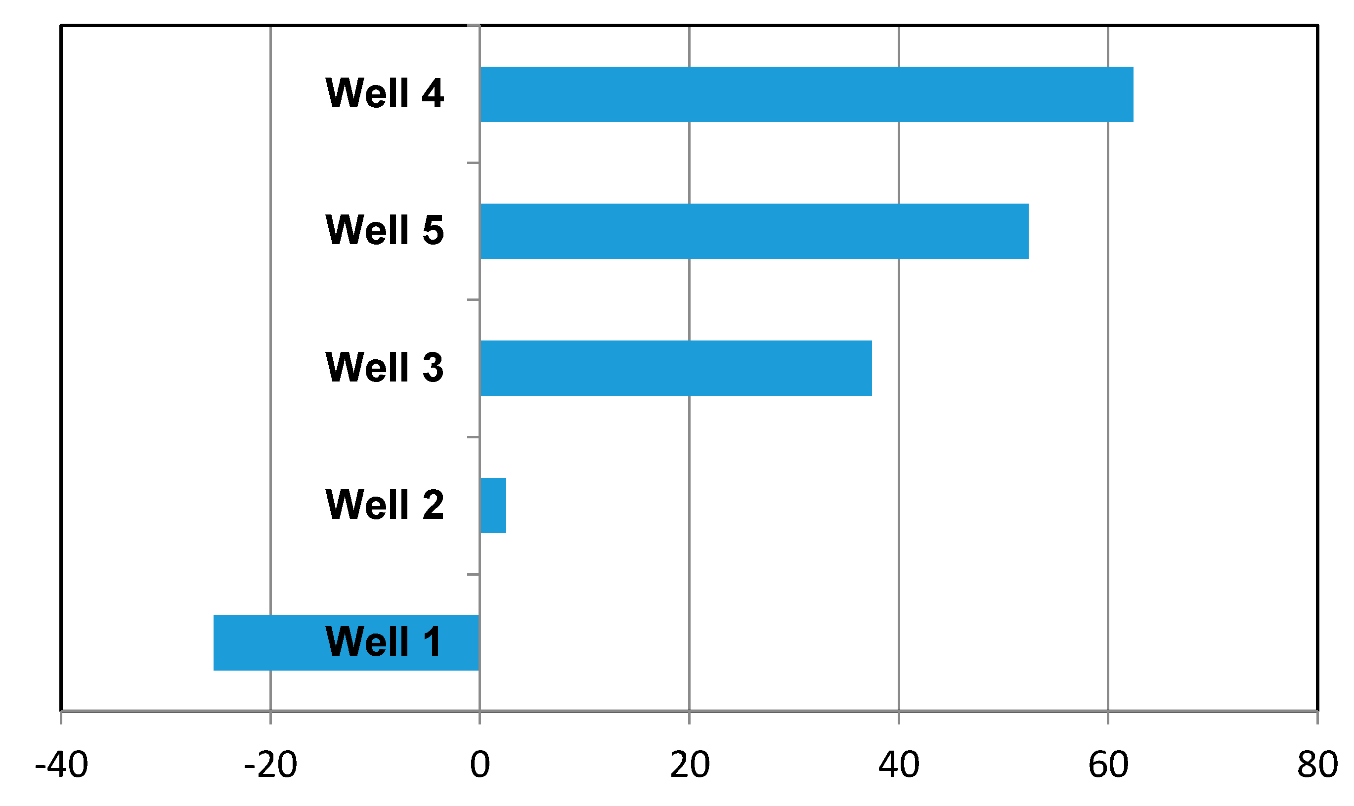
The economic evaluation based on the values given in Table 3 resulted in maximum NPV values of −25.4, 2.5, 37.4, 62.4, and 52.4 MMGBP for well 1 to 5, respectively (Figure 8).
Considering the positive value of NPV as the project successfulness criterion, one well out of five failed to be commercial due to heterogeneity as the design of the wells were almost identical. This corresponded to the value of 20% for RCF obtained in the previous section.
4. Conclusions
Hydraulic fracturing economical evaluation at the low energy price era is more complicated and an appropriate decision-making process for such projects requires integration of technical forecasting including uncertainty analysis with economical models. Such models are very time consuming to implement if they include three-dimensional reservoir property variation.
An empirical approach was suggested to capture the heterogeneity using well-test analysis and net-pressure-match interpretations (HIF). Then a new set of decline curve analysis formulas linked HIF to forecasting. This paper proposed a time-efficient workflow to capture the uncertainty of HIF using real data from a tight field in the Southern North Sea, a set of formulas for NPV calculation including commercial cut-off and calculation of NPV probability distribution, and, finally, a new insightful parameter called the Risk of Commercial Failure (RCF) due to heterogeneity for hydraulic fracturing projects. RCF represents the risk of the project due to heterogeneity. RCF has been calculated as 20% for the next phase development of a real field case.
Author Contributions
Sina Rezaei Gomari, and Farhad Nabhani were directors of the project. Hadi Parvizi was responsible to build the models and write the first draft of this paper. Abolfazl Dehghan Monfared was also responsible for some constructive suggestions for the economic models.
Conflicts of Interest
The authors declare no conflicts of interest.
References
- Arthur, J.D.; Bohm, B.K.; Coughlin, B.J.; Layne, M.A.; Cornue, D. Evaluating the Environmental Implications of Hydraulic Fracturing in Shale Gas Reservoirs. In Proceedings of the SPE Americas E&P Environmental and Safety Conference, San Antonio, TX, USA, 23–25 March 2009. [Google Scholar]
- Phatak, A.; Kresse, O.; Nevvonen, O.V.; Abad, C.; Cohen, C.-E.; Lafitte, V.; Abivin, P.; Weng, X.; England, K.W. Optimum Fluid and Proppant Selection for Hydraulic Fracturing in Shale Gas Reservoirs: A Parametric Study Based on Fracturing-to-Production Simulations. In Proceedings of the SPE Hydraulic Fracturing Technology Conference, The Woodlands, TX, USA, 4–6 February 2013. [Google Scholar]
- Denney, D. Evaluating Implications of Hydraulic Fracturing in Shale-Gas Reservoirs. Petroleum Technol. 2009, 61, 53–54. [Google Scholar] [CrossRef]
- Tan, P.; Jin, Y.; Han, K.; Hou, B.; Chen, M.; Guo, X.; Gao, J. Analysis of hydraulic fracture initiation and vertical propagation behavior in laminated shale formation. Fuel 2017, 206, 482–493. [Google Scholar] [CrossRef]
- Xu, C.; Li, P.; Lu, D. Production performance of horizontal wells with dendritic-like hydraulic fractures in tight gas reservoirs. J. Pet. Sci. Eng. 2017, 148, 64–72. [Google Scholar] [CrossRef]
- Lai, F.; Li, Z.; Wang, Y. Impact of water blocking in fractures on the performance of hydraulically fractured horizontal wells in tight gas reservoir. J. Pet. Sci. Eng. 2017, 156, 134–141. [Google Scholar] [CrossRef]
- Murtaza, M.; Al Naeim, S.; Waleed, A. Design and Evaluation of Hydraulic Fracturing in Tight Gas Reservoirs. In Proceedings of the SPE Saudi Arabia Section Technical Symposium and Exhibition, Al-Khobar, Saudi Arabia, 19–22 May 2013. [Google Scholar]
- Vos, B.; Shaoul, J.R.; de Koning, K.J. Southern North Sea Tight-Gas Field Development Planning Using Hydraulic Fracturing. In Proceedings of the EUROPEC/EAGE Conference and Exhibition, Amsterdam, The Netherlands, 8–11 June 2009. [Google Scholar]
- Antoci, J.C.; Anaya, L.A. First Massive Hydraulic Fracturing Treatment in Argentina. In Proceedings of the SPE Latin American and Caribbean Petroleum Engineering Conference, Buenos Aires, Argentina, 25–28 March 2001. [Google Scholar]
- Shaoul, J.R.; Ross, M.J.; Spitzer, W.J.; Wheaton, S.R.; Mayland, P.J.; Singh, A.P. Massive Hydraulic Fracturing Unlocks Deep Tight Gas Reserves in India. In Proceedings of the European Formation Damage Conference, Scheveningen, The Netherlands, 30 May–1 June 2007. [Google Scholar]
- Parvizi, H.; Rezaei-Gomari, S.; Nabhani, F.; Dastkhan, Z.; Feng, W.C. A Practical Workflow for Offshore Hydraulic Fracturing Modelling: Focusing on Southern North Sea. In Proceedings of the EUROPEC 2015, Madrid, Spain, 1–4 June 2015. [Google Scholar]
- Al-zarouni, A.Y.A.A.; Ghedan, S.G. Paving the Road for the First Hydraulic Fracturing in Tight Gas Reservoirs in Offshore Abu Dhabi. In Proceedings of the SPE Middle East Unconventional Gas Conference and Exhibition, Abu Dhabi, UAE, 23–25 January 2012. [Google Scholar]
- Rodgerson, J.L. Impact of Natural Fractures in Hydraulic Fracturing of Tight Gas Sands. In Proceedings of the SPE Permian Basin Oil and Gas Recovery Conference, Midland, TX, USA, 21–23 March 2000. [Google Scholar]
- Maxwell, S.C. Assessing the Impact of Microseismic Location Uncertainties on Interpreted Hydraulic Fracture Geometries. In Proceedings of the SPE Annual Technical Conference and Exhibition, New Orleans, LA, USA, 4–7 October 2009. [Google Scholar]
- Bahrami, H.; Rezaee, R.; Clennell, B. Water blocking damage in hydraulically fractured tight sand gas reservoirs: An example from Perth Basin, Western Australia. J. Pet. Sci. Eng. 2012, 88, 100–106. [Google Scholar] [CrossRef]
- Parvizi, H.; Rezaei-Gomari, S.; Nabhani, F.; Turner, A.; Feng, W.C. Hydraulic Fracturing Performance Evaluation in Tight Sand Gas Reservoirs with High Perm Streaks and Natural Fractures. In Proceedings of the EUROPEC 2015, Madrid, Spain, 1–4 June 2015. [Google Scholar]
- Westwood, R.F.; Toon, S.M.; Cassidy, N.J. A sensitivity analysis of the effect of pumping parameters on hydraulic fracture networks and local stresses during shale gas operations. Fuel 2017, 203, 843–852. [Google Scholar] [CrossRef]
- Wilson, A. Hydraulic-Fracture Design: Optimization under Uncertainty. J. Pet. Technol. 2015, 67. [Google Scholar] [CrossRef]
- Bai, M. Risk and Uncertainties in Determining Fracture Gradient and Closure Pressure. In Proceedings of the 45th U.S. Rock Mechanics/Geomechanics Symposium, San Francisco, CA, USA, 26–29 June 2011. [Google Scholar]
- Durant, B.; Abualfaraj, N.; Olson, M.S.; Gurian, P.L. Assessing dermal exposure risk to workers from flowback water during shale gas hydraulic fracturing activity. J. Nat. Gas Sci. Eng. 2016, 34, 969–978. [Google Scholar] [CrossRef]
- Harding, N.R. Application of Stochastic Prospect Analysis for Shale Gas Reservoirs. In Proceedings of the SPE Russian Oil and Gas Technical Conference and Exhibition, Moscow, Russia, 28–30 October 2008. [Google Scholar]
- Willigers, B.J.; Bratvold, R.B.; Bickel, J.E. Maximizing the Value of Unconventional Reservoirs by Choosing the Optimal Appraisal Strategy. SPE Reserv. Eval. Eng. 2017, 20. [Google Scholar] [CrossRef]
- Williams-kovacs, J.; Clarkson, C.R. Using Stochastic Simulation to Quantify Risk and Uncertainty in Shale Gas Prospecting and Development. In Proceedings of the Canadian Unconventional Resources Conference, Calgary, AB, Canada, 15–17 November 2011. [Google Scholar]
- Liang, B.; Khan, S.; Puspita, S.D.; Tran, T.; Du, S.; Blair, E.; Rives, S. Improving Unconventional Reservoir Factory-Model Development by an Integrated Workflow with Earth Model, Hydraulic Fracturing, Reservoir Simulation and Uncertainty Analysis. In Proceedings of the Unconventional Resources Technology Conference (URTEC), San Antonio, TX, USA, 1–3 August 2016. [Google Scholar]
- Thiele, M.R.; Batycky, R.P. Evolve: A Linear Workflow for Quantifying Reservoir Uncertainty. In Proceedings of the SPE Annual Technical Conference and Exhibition, Dubai, UAE, 26–28 September 2016. [Google Scholar]
- Hosseini, B.K.; Chalaturnyk, R.J. Streamline-Based Reservoir Geomechanics Coupling Strategies for Full Field Simulations. In Proceedings of the 14th European Conference on the Mathematics of Oil Recovery, Catania, Italy, 8–11 September 2014. [Google Scholar]
- Thiele, T.M.R.; Batycky, R.P. Using Streamline-Derived Injection Efficiencies for Improved Waterflood Management. SPE Reserv. Eval. Eng. 2006, 9, 187–196. [Google Scholar] [CrossRef]
- Jesmani, M.; Hosseini, B.K.; Chalaturnyk, R.J. Use of Streamlines in Development and Application of a Linearized Reduced-Order Reservoir Model. In Proceedings of the 9th International Geostatistics Congress, Oslo, Norway, 11–15 June 2012. [Google Scholar]
- Hosseini, B.K.; Chalaturnyk, R.J. A Domain Splitting-Based Analytical Approach for Assessing Hydro-thermo-geomechanical Responses of Heavy Oil Reservoirs. SPE J. 2016, 22. [Google Scholar] [CrossRef]
- Parvizi, H.; Rezaei-Gomari, S.; Nabhani, F. Robust and Flexible Hydrocarbon Production Forecasting Considering the Heterogeneity Impact for Hydraulically Fractured Wells. Energy Fuels 2017, 31, 8481–8488. [Google Scholar] [CrossRef]
- Parvizi, H.; Rezaei-Gomari, S.; Nabhani, F.; Turner, A. Evaluation of heterogeneity impact on hydraulic fracturing performance. J. Pet. Sci. Eng. 2017, 154, 344–353. [Google Scholar] [CrossRef]
- Jonsbråten, T.W. Oil field optimization under price uncertainty. J. Oper. Res. Soc. 1998, 49, 811–818. [Google Scholar] [CrossRef]
- Goel, V.; Grossmann, I.E. A stochastic programming approach to planning of offshore gas field developments under uncertainty in reserves. Comput. Chem. Eng. 2004, 28, 1409–1429. [Google Scholar] [CrossRef]
- Ozdogan, U.; Horne, R.N. Optimization of Well Placement under Time-Dependent Uncertainty. SPE Reserv. Eval. Eng. 2006, 9. [Google Scholar] [CrossRef]
- PremierOil, Proposed acquisition of the EPUK Group Circular to Shareholders and Notice of General Meeting. Available online: http://www.premier-oil.com/premieroil/dlibrary/panda/Eva-FINAL-CIRCULAR.pdf (accessed on 20 July 2017).
Figure 1.
Selection of commercial cut off for a pre-specified value of Heterogeneity Impact Factor (HIF).
Figure 1.
Selection of commercial cut off for a pre-specified value of Heterogeneity Impact Factor (HIF).

Figure 2.
Variation of net present value (NPV) over time for change in different economic parameters and HIF. (a) End of the 5th year of production; (b) End of the 10th year of production; (c) End of the 15th year of production; (d) End of the 20th year of production.
Figure 2.
Variation of net present value (NPV) over time for change in different economic parameters and HIF. (a) End of the 5th year of production; (b) End of the 10th year of production; (c) End of the 15th year of production; (d) End of the 20th year of production.

Figure 3.
NPV sensitivity analysis showing the significant role of HIF parameter.

Figure 4.
Workflow of Risk of Commercial Failure (RCF) calculation.

Figure 5.
NPV versus production time for base case (HIF = 1).

Figure 6.
Commercial cut-off years after production versus Heterogeneity Impact Factor.

Figure 7.
Cumulative probability distribution of NPV.

Figure 8.
Maximum NPV for five wells drilled in Babbage Field.


Table 1.
The uncertainty range for the sensitivity analysis.
| Input Parameter | Low Value | Mid Value | High Value | Unit |
|---|---|---|---|---|
| Capital Expenditure (CAPEX) | 30 | 45 | 60 | MMGBP |
| Operational Expenditure (OPEX) | 1 | 2 | 4 | MMGBP/Year |
| HIF | 0.35 | 1 | 1.75 | - |
| I (discount rate) | 0.05 | 0.1 | 0.15 | Yearly |
| GBPg (gas price) | 4 | 5 | 6 | GBP/MSCF |
Table 2.
Sensitivity analysis results. Different values are color coded with colors ranging from red (representing the lowest NPV value) to dark green (representing the highest NPV value).
Table 2.
Sensitivity analysis results. Different values are color coded with colors ranging from red (representing the lowest NPV value) to dark green (representing the highest NPV value).
| Parameters | Maximum NPV [MMGBP] | ||
|---|---|---|---|
| Low Value | Mid Value | High Value | |
| HIF | −25.4 | 37.4 | 62.4 |
| GBP_g (gas price) | 17.2 | 37.4 | 58 |
| I (Discount Rate) | 25.3 | 37.4 | 56 |
| CAPEX | 22.4 | 37.4 | 52.4 |
| OPEX | 21.3 | 37.4 | 48.7 |
Table 3.
Economical and forecasting assumptions.
| INPUT Parameter | Value | Unit |
|---|---|---|
| CAPEX per well | 45 | MMGBP |
| OPEX per well in this field | 2 | MMGBP |
| qi | 25,000 | MSCF/d |
| GBP_g (gas price) | 5 | GBP/MSCF |
| I (Discount rate) | 0.1 | Yearly |
| D | 4.2 | % Monthly |
Table 4.
Matched HIF per well.
| Well No | HIF |
|---|---|
| 1 | 0.35 |
| 2 | 0.65 |
| 3 | 1 |
| 4 | 1.75 |
| 5 | 1.4 |
Table 5.
Values of different parameters utilized to calculate gas production.
| Well No | HIF | qmi | Dmi | b |
|---|---|---|---|---|
| 1 | 0.35 | 8750 | 4.2 | 0.7 |
| 2 | 0.65 | 16,250 | 4.2 | 0.7 |
| 3 | 1 | 25,000 | 4.2 | 0.7 |
| 4 | 1.75 | 43,750 | 7.35 | 0.7 |
| 5 | 1.4 | 35,000 | 1.95 | 0.7 |
© 2018 by the authors. Licensee MDPI, Basel, Switzerland. This article is an open access article distributed under the terms and conditions of the Creative Commons Attribution (CC BY) license (http://creativecommons.org/licenses/by/4.0/).
Share and Cite
MDPI and ACS Style
Parvizi, H.; Rezaei Gomari, S.; Nabhani, F.; Dehghan Monfared, A. Modeling the Risk of Commercial Failure for Hydraulic Fracturing Projects Due to Reservoir Heterogeneity. Energies 2018, 11, 218. https://doi.org/10.3390/en11010218
AMA Style
Parvizi H, Rezaei Gomari S, Nabhani F, Dehghan Monfared A. Modeling the Risk of Commercial Failure for Hydraulic Fracturing Projects Due to Reservoir Heterogeneity. Energies. 2018; 11(1):218. https://doi.org/10.3390/en11010218
Chicago/Turabian StyleParvizi, Hadi, Sina Rezaei Gomari, Farhad Nabhani, and Abolfazl Dehghan Monfared. 2018. "Modeling the Risk of Commercial Failure for Hydraulic Fracturing Projects Due to Reservoir Heterogeneity" Energies 11, no. 1: 218. https://doi.org/10.3390/en11010218
Note that from the first issue of 2016, this journal uses article numbers instead of page numbers. See further details here.