Article

Electric Arc Furnace Modeling with Artificial Neural Networks and Arc Length with Variable Voltage Gradient

by
Raul Garcia-Segura
1,
Javier Vázquez Castillo
1,*,
Fernando Martell-Chavez
2,
Omar Longoria-Gandara
3 and
Jaime Ortegón Aguilar
1
1
Deparment of Engineering, University of Quintana Roo, Chetumal 77019, Mexico
2
Research Center in Optics, Aguascalientes 20200, Mexico
3
Department of Electronics, Systems and IT, ITESO, Tlaquepaque 45604, Mexico
*
Author to whom correspondence should be addressed.
Energies 2017, 10(9), 1424; https://doi.org/10.3390/en10091424
Submission received: 13 June 2017 / Revised: 3 August 2017 / Accepted: 3 August 2017 / Published: 16 September 2017
(This article belongs to the Section F: Electrical Engineering)

Abstract

:
Electric arc furnaces (EAFs) contribute to almost one third of the global steel production. Arc furnaces use a large amount of electrical energy to process scrap or reduced iron and are relevant to study because small improvements in their efficiency account for significant energy savings. Optimal controllers need to be designed and proposed to enhance both process performance and energy consumption. Due to the random and chaotic nature of the electric arcs, neural networks and other soft computing techniques have been used for modeling EAFs. This study proposes a methodology for modeling EAFs that considers the time varying arc length as a relevant input parameter to the arc furnace model. Based on actual voltages and current measurements taken from an arc furnace, it was possible to estimate an arc length suitable for modeling the arc furnace using neural networks. The obtained results show that the model reproduces not only the stable arc conditions but also the unstable arc conditions, which are difficult to identify in a real heat process. The presented model can be applied for the development and testing of control systems to improve furnace energy efficiency and productivity.

1. Introduction

An electric arc furnace (EAF) [1] is an industrial device used for steel production and other important applications (e.g., [2]). The actual energy used in EAFs depends on the quality and conditions of the charge materials (scrap, direct reduced iron (DRI), and others), the amount of slag, and the total time of the heat. EAF facilities contribute to a great proportion (estimated to be 31%) of the world’s steel production [3]. EAFs work in very large electrical loads ranging from several megavolt amperes (MVA) to 250 MVA in modern facilities, which means that small improvements in efficiency represent significant electrical energy savings. In this sense, many researchers have been focusing their efforts on improving the efficiency in EAFs; for example, Trejo et al. [4] analyzed the components that decrease furnace efficiency and introduced a novel estimation of electrical and cooling losses in EAFs. Kirschen et al. [5] presented a model of EAF energy efficiency which is based on closed mass and energy balance of the EAF melting process, and Hocine et al. [6] presents an improvement of EAF operation with appropriate models and discusses all the factors that play a role in the melting process. In [7], the effect of voltage flicker on the systems with EAF, random, and sinusoidal voltage flickers are studied, which made it possible to introduce a new more realistic time domain model for EAFs.
On the other hand, in alternating current (AC) furnaces, the power system consists of a power transformer with variable tap and sometimes a series reactor on the primary side to increase the system reactance. The electric arcs are controlled by electrode displacement. The arc regulation system drives the electrodes up and down to control a desired current or impedance per each phase. In the heat process, the harmonic distortion of the voltage and current signals varies from higher total harmonic distortion (THD) at initial bore-down and early melting to a final lowest THD value during the refining and heating stages. The amount of harmonic generation is therefore dependent on the stage of the melting process [6,8,9].
In this sense, an EAF is then a stochastic process which has a certain aperiodicity level that changes cycle by cycle, which greatly increases the voltage and current distortion in magnitude, phase, and frequency. There are several reasons why the electrical measurement of voltage and currents yields time-varying values even in the root mean square (RMS) values; one involves the changes in the high-power transformer and reactor tap, the second has to do with the continuous movement of the electrodes, and the third and most significant reason is due to the changing process conditions (i.e., the dynamic change in the arc atmosphere that is influenced mainly by the melting process). It may be very chaotic in the presence of scrap, and tends to be more stable during the heat stage called flat bath.
Today, there are several studies in the open literature addressing the problem of modeling EAFs with an artificial neural network (ANN) [10,11,12,13,14,15]. In this sense, inputs of interest are passed through an ANN and transformed by using activation functions to produce outputs. For example, in [10], the electric arc furnace parameters of a selected EAF model are computed and estimated via ANNs. In [11,12], the modeling and prediction of EAF based on ANN and chaos theory is presented with a radial basis function neural network used to predict the arc voltage of the EAF. Chang et al. [13] presents an accurate neural-network-based method for modeling the highly nonlinear voltage–current characteristics of the EAF. In [14], the modeling of electrical energy consumption in an EAF is presented using artificial neural networks. The multilayer perceptron architecture 5-5-1 with a hyperbolic tangent function in the hidden layer and a linear function in the output layer was used as an optimal neural network model. Baumert et al. [15] presents one of the first studies for carrying out the dynamic modeling of the electric arc furnace process using artificial neural networks.
In this paper, a new methodology for modeling EAFs is presented which considers time-varying arc lengths as relevant input parameters for the arc furnace model for the generation of voltage and current waveforms. Based on actual voltages and current measurements taken from an arc furnace, it was possible to estimate an arc length suitable for modeling the arc furnace using neural networks. Moreover, the inclusion of the varying arc length by means of a variable voltage gradient makes it possible to capture the dynamic behavior of the system, allowing for a more real and accurate waveform reproduction of the EAF system model.
The EAF model proposed in this study is relevant since it can be used to reproduce the behavior of the arc furnace process variables in simulation schemes such as hardware in the loop (HIL), where the real control system can be tested with a simulated process. In this sense, advanced control techniques and strategies applying energy efficiency criteria could be developed and tested using the present EAF model prior to their implementation in a real furnace.
The rest of the paper is organized as follows: Section 2 presents the background related to the ANN and the EAF modeling. The introduced methodology is analyzed in Section 3. Section 4 presents the ANN-EAF model simulation results, and Section 5 discusses the EAF modeling in the context of widely-used ANN-EAF implementations. Finally, the conclusion is presented in Section 6.

2. Background

2.1. Electric Arc Furnace (EAF) Model

Today, several approaches for modeling EAF subsystems have been studied and reported in the literature. For example, Figure 1 shows the electrical circuit of the EAF which is modeled with reactance and resistance elements within a three-phase system that includes an embedded transformer. This transformer is fed with high voltage, which delivers energy to the electrodes. Each electrode is connected to one phase having its own resistance and inductance values corresponding to the materials of the conductor. As seen in Figure 1, the load (e.g., the electric arcs) is represented as variable resistances in the EAF model. In order to keep the electric arcs burning, the electrodes’ currents need to be controlled by means of an electrode control system.

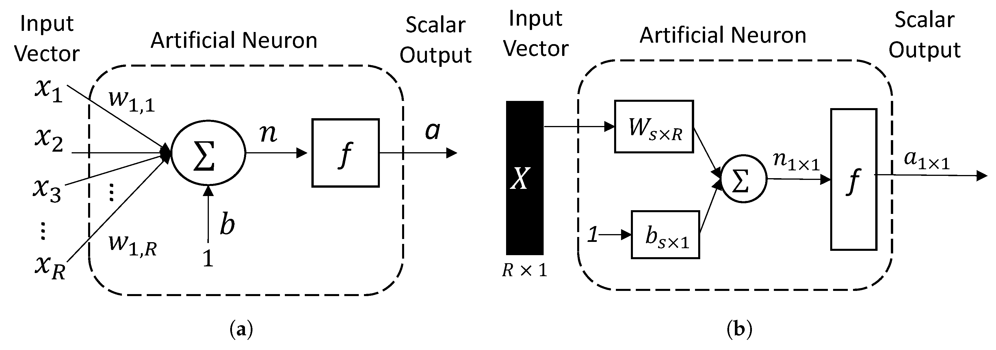
2.2. Artificial Neural Network

An ANN is a system that allows inputs x and outputs y of interest to be related via a mathematical function [16]. The simplest element in an ANN is a neuron; for example, Figure 2 shows a basic neural network that consists of inputs and outputs, where the inputs are weighted, added, and activated to generate the outputs. In this sense, a neuron can be mathematically represented as follows:
a = f i = 1 n x i w i + b ,
where x i are the inputs, w i are the weights, b is a bias, and f · represents the activation function; additionally, it is possible to classify the neurons as the input, hidden, and output layers. All the layers are interconnected, and the weights are optimally computed using a cost function. In general, the sum-squared error is minimized in the optimization process or ANN training (see [17] for more details about ANNs).

2.3. ANN Training Algorithm

There are two ways to train an ANN: incremental and batch training. In incremental training, the weights and biases of the network are updated as an input is presented (updated) to the ANN. In batch training, the weights and biases are only updated after all the inputs are presented. Depending on the application, the style of training is chosen; usually, incremental training is used for adaptive filter applications; however, batch training is the most commonly used. Among the training algorithms in batch mode, the backpropagation algorithm is the principal method used for computing the weights, where the optimization scheme moves from the highest layer to the lowest of the ANN in opposition to the neuron activation through the network (see [17] for more details about ANN training algorithms).

2.4. Theoretical Arc Length Calculation

For modeling purposes, the arc length is the signal preferred to be chosen as the input for the model, since the electrode control system modifies the electrode displacement, and therefore the arc length. To obtain the arc length, it is necessary to calculate the arc voltage by solving the electric circuit of the EAF shown in Figure 1. After that, the effective or root mean square (RMS) value of the arc voltage is calculated per each phase according to:
l a r c = E V a r c 40 k
where l a r c is the arc length, E V a r c is the RMS voltage of the arc, and k is the gradient value [18]. According to the open literature, the k value is fixed at 11.5 Volts/cm, which is often assumed to remain constant in all stages of the melting process (stationary behavior). On the other hand, as can be seen in Equation (2), the arc length depends almost exclusively on the arc voltage, appearing to be almost independent of the current. In this paper, the use of variable voltage gradients is proposed for calculating the arc lengths allowing the simulation of the most realistic EAF models and waveform generation of the melting process. The modeling can be benefited by considering the voltage gradient as a variable parameter within a certain range. In this way, most of the randomness of the voltage-current relationship can be attributed to the voltage gradient, and the arc length can have a more linear relationship with the arc voltage.

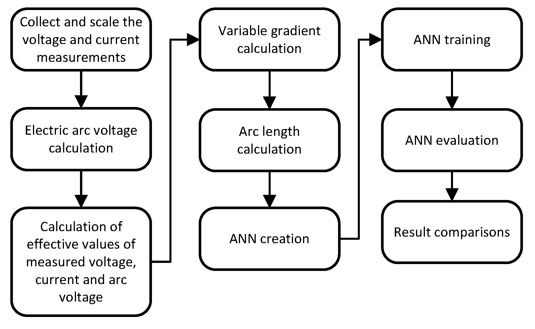
3. Proposed Methodology

The proposed methodology for modeling the EAF using ANNs is presented in Figure 3, which consists of nine stages. In order to corroborate the accuracy of the proposed methodology, a case study was carried out according to the following configuration parameters: the voltage and current measurements were gathered from the secondary side of the transformer using a digital acquisition system (National Instruments Compact RIO) with a sampling period of 60 μ s in an operating EAF of 120 tons.
It is important to note that the calculated RMS values need be decimated in order to reduce the quantity of data to work with; then, a cycle per each seven and a half cycles (2048 samples) is selected for processing. The principal stages of the methodology are described in the following subsections.

3.1. Arc Voltage Calculation

In this stage, the electric circuit of the EAF is solved (Figure 1), in order to obtain the arc voltage ( v a r c ) per phase, as follows:
v a r c R = v R N v E A F R
where v R N is the R phase voltage to neutral, and v E A F R is the voltage of the EAF electric circuit in the R phase. The arc volage ( v a r c ) in the S phase ( v a r c S ) and the T phase ( v a r c T ) can be calculated using the same procedure. The EAF electric circuit is represented as an inductor and a resistance of the conductor cables of Figure 1. Thus, Equation (3) is rewritten as:
v a r c R = v R N L d i d t i R = v R N X L ω d i d t i R
where the inductance L = X L / ω , ω is the frequency in radians, and X L is the short circuit reactance, which usually has values in the range from 3 to 4 Ω , and the resistance R has values in the range from 0.4 to 0.5 Ω . Furthermore, X L and R generally maintain a relation from 1 to 10 or 1 to 12. In this sense, the arc voltage can be reformulated as:
v a r c R = v R N 3.6 377 d i d t i ( 0.45 )
Equations (3)–(5) are to obtain the values of phase R; equivalent expressions apply to phases T and S. For the calculations of voltages v R N , v S N , and v S N , it is necessary to obtain the v N G (neutral to ground voltage), which according to theory must be zero for balanced circuits; nevertheless, in this case, this voltage has a magnitude different from zero.

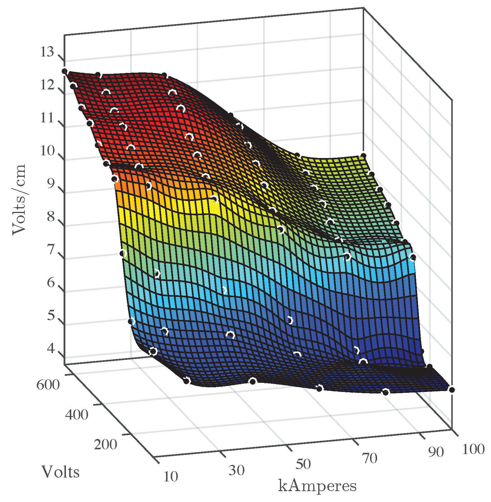
3.2. Arc Length Calculation via Variable Voltage Gradients

In order to compute the arc length in Equation (2), in this study, the effective voltage E V a r c is computed per semi cycle and the dynamic behavior in the EAF model is incorporated by a variable voltage gradient in the arc length calculation. However, in the EAF modeling, some relations about the voltage gradient must be established in terms of voltages and currents.
One problem that arises in the modeling is that the voltage gradient changes almost every heating cycle , and behaves with high variance during initial bore down and early melting. More stationary values are present during late melting and refining. Figure 4 shows the voltage gradients of the introduced case study, which depend on the voltage and current RMS values. The gradient variable represents the non-stationary behavior during the fusion process in the arc model. In this sense, the parameter k in Equation (2) needs to be updated each semi-cycle. The values were fitted and adjusted using data from experimental measurements reported in [9]. The data shown in Figure 4 can be interpolated (e.g., using a piecewise polynomial approximation technique) and represented as a surface function that can generate a voltage gradient (Volts/cm) corresponding to a value per each volt-ampere combination.

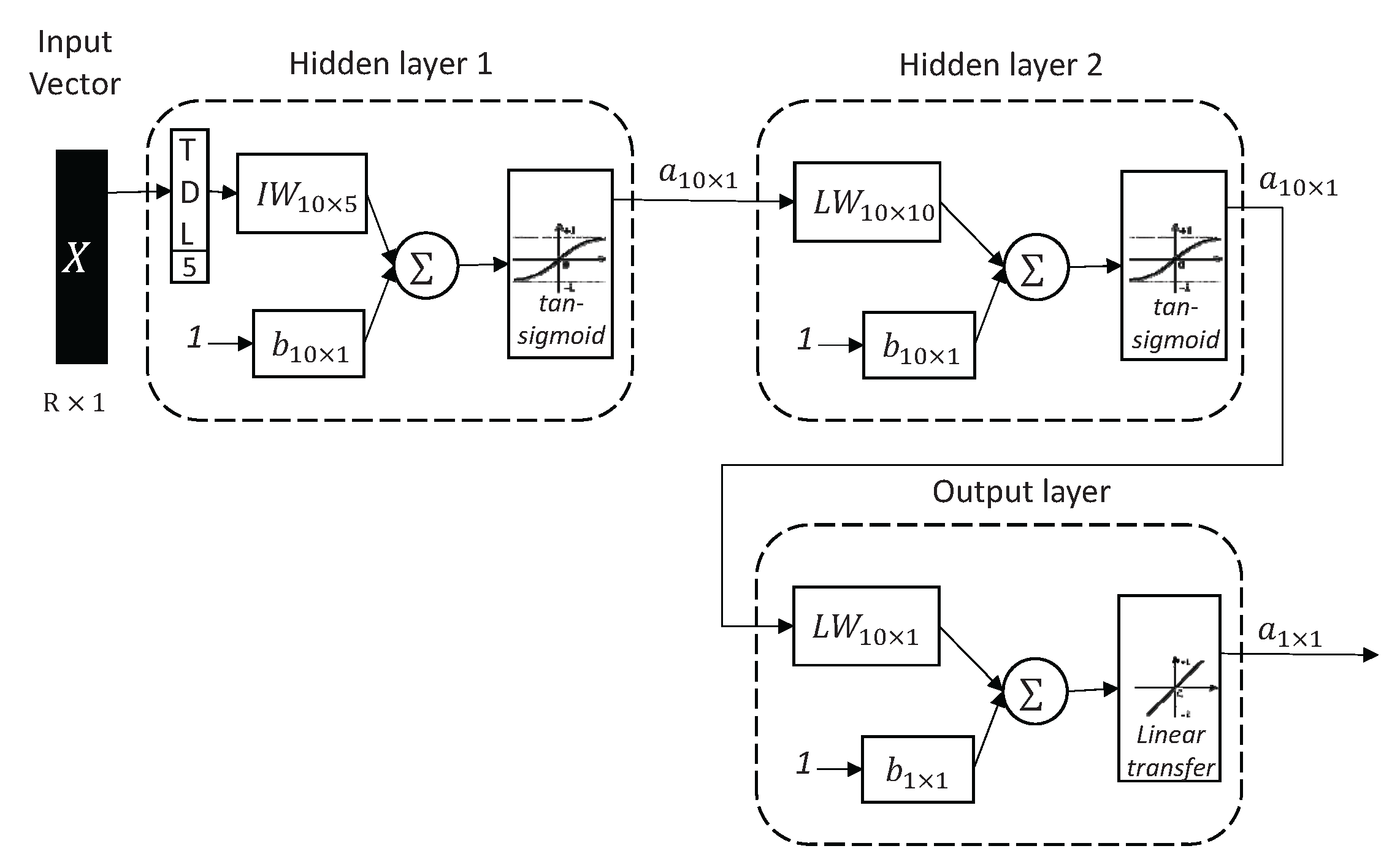
3.3. Proposed ANN Architecture

In order to reproduce the melting process behavior in the EAF, several tests were carried out with different ANN structures. The study of the ANN structures was carried out considering the training error as the mean square error, and using different configurations of the hidden layers (1, 2, and 3), as well as different numbers of neurons per layer (5, 10, 15, and 20). After an analysis of the ANN’s performance, it was decided to work with a feedforward dynamic neural network focused on delays at the inputs. This ANN belongs to a general category of focused networks, where the dynamic behavior only appears in the input layer (see [17] for more details).
The ANN structure used in the study case is shown in Figure 5, and it considers a delay of five samples. The ANN is composed of two hidden layers with ten neurons using tan-sigmoid transfer functions. The output layer embeds one neuron, which uses a linear transfer function. The ANN was implemented in Matlab, using the Neural Net Toolbox; moreover, it was trained using the Levenberg-Marquardt (LM) algorithm [17]. The input vector is built using the arc length with a tapped delay line with delays from 1 to 5; the output value is the voltage or current, depending on the experiment. There are six neural nets, corresponding to the three stages with current or voltage as the output value. For each neural net, the data was divided in training, validation, and test set, with 70, 15, and 15%, respectively. The data consist of 2048 samples per stage. These data belong to a representative section of the corresponding stage.

4. ANN Experimental Results

Once the RMS values per semi-cycle of the voltage and current waveform measurements in the melting process are computed (see Figure 6a,b for phase R), three main stages of the melting process are identified: unstable, intermediate, and stable stage. The unstable stage is defined from 0 to 800 s; the intermediate stage—where the current grows continuously—from 801 to 1400 s. Finally, the stable stage is defined from 1401 s to the end of the melting.
Figure 7 shows the arc length estimations using the introduced variable gradient values. As can be seen, the length of the electric arc changes as time passes and the voltages and currents vary.
As was mentioned in the introduced modeling strategy, the arc length was chosen as an input parameter in the ANN structure in order to generate voltage and current waveforms. The comparison results of the EAF modeling are shown in Figure 8. As can be seen, the identification achieved with the ANN structure (gray dotted line) approaches the real measurements (black line). It is important to mention that one advantage of this model is that implementation could be relatively easy to develop on hardware in terms of memory resources. The ANN used in this study consists of 181 values distributed over 160 weights, 21 biases, and 2 kinds of transfer functions. The transfer functions can be designed via piecewise polynomial approximation techniques [19,20].
In order to corroborate the precision of the ANN-EAF model, a goodness of fit test was carried out [21]. This test considered the comparison between the estimated output and the desired output (see Figure 8); in this sense, the fitness level reached during the unstable stage was 95.5% and 98.5% for the voltage and current outputs, respectively. In the intermediate stage, the adjustment level reached was 99.8% for the voltage output and 99.7% for the current output. Finally, 97.1% and 99.76% of adjustment levels were reached in the stable stage (voltage and current, respectively). In this sense, by having analyzed the performance of the ANNs in terms of voltage and current outputs, and because variable voltage gradients were used to carry out the proposed methodology, it is possible to conclude that the ANN model can generate voltage and current waveforms which converge with the desired outputs accurately, allowing the modeling of EAF systems.
On the other hand, it must be mentioned that a direct comparison among the different ANN structures that have been proposed for modeling the EAF is difficult to carry out. As was seen in Section 1, the EAF models are analyzed with different methods, techniques, and focuses; however, the common point is that all the models have tried to capture the realistic behavior of the EAF via the inclusion of important variables in the models such as arc length, position of electrodes, and topology of the external circuits, among others.

5. Discussion

This paper proposes the generation of voltage and current waveforms via the use of ANNs. In addition, a new computing strategy for calculating the arc lengths is introduced in Section 3.2, where it serves as input for the ANN system model. The arc lengths computed via Equation (2) embed the non-stationary voltage-current behavior persistent in real EAF systems, which allows more real waveforms to be generated for use in EAF simulators. The arc length computation depends on the voltage gradients (dynamic behavior) impacting the ANN output toward a more real and accurate voltage-current waveform generation. In their work , López et al. [10] computed the arc lengths using nonlinear differential equations, which is a fixed structure with current input parameters. Once the arc length is obtained, it is passed to a new model in order to compute the electric arc voltage. Finally, the parameters of the blocks for obtaining the arc length and the electric arc voltage are approximated via a feedforward ANN structure. The voltage generation methodology presented in [10] differs from our proposal in the sense that we are using variable voltage gradients for calculating the arc lengths (a new dynamic formula), which can be used in EAF systems to simulate real electric arc voltage in order to implement EAF control strategies. In [11,12], an ANN was used to estimate the arc length voltage in an EAF system, which can be used to estimate the future state of arc furnaces for control purposes. The methodology used considers the use of chaotic time series via an embedding theorem. Basically, the ANN is used for mapping (radial basis function networks) or carrying out a function transformation. This methodology can produce accurate arc voltages; however, this methodology does not compute the EAF arc length. In the same topic, Chang et al. [13] present a method based on ANN for modeling the highly nonlinear voltage-current characteristics of an EAF. In this study, a radial basis function ANN (RBFANN) is used to perform curve fitting by using a family of basis function to relate the inputs and outputs. For this aim, a RBFANN and lookup tables (LUTs) are used to describe the relation between the EAF current and the voltage. In this case, the RBFANN is used for expanding the stochastic process and the LUTs allocate the parameters related to the dynamic characteristics of the EAF current-voltage waveforms. In our methodology, the dynamic current-voltage is computed via Equation (2), which lets us avoid the use of additional hardware/software resources to achieve accuracy in the EAF waveform reproduction. In the case of [14], the paper reports the importance of the charge material in the EAF, which impacts the electrical energy consumed. In this respect, the ANN relates the effect of the content of carbon, chromium, nickel, silicon, and iron (ANN inputs) with respect to the EAF’s electrical energy consumption (ANN output). Finally, Baumert et al. [15] describes an ANN model for predicting electrical energy consumption, which differs from our proposal. After analyzing the different state-of-the-art ANN-EAF applications (widely cited in the open literature), it is possible to conclude that many ANN structures have been used for tackling different issues in EAF modeling, which makes it difficult to carry out a direct comparison among ANN-EAF models.

6. Conclusions

In this paper a new methodology was presented for modeling an EAF via ANNs and arc length. This introduced methodology considers the time variation of the arc length in the arc furnace model as an input parameter, which is calculated using variable voltage gradients. The convergence of the system model obtained was corroborated by carrying out a case study and using measurements gathered from an EAF under operation during the whole melting process (unstable, intermediate, and stable stages). Comparison results show that the ANNs can generate voltage and current waveforms which converge with outputs gathered from the EAF. The inclusion of the varying arc length by means of a variable voltage gradient makes it possible to capture the dynamic behavior of the system and generate a more real and accurate waveform in the EAF system model. The model presented here is useful for developing and testing control techniques for the power control and the arc regulation systems required by the electric arc furnace, and in this way it improves the furnace energy efficiency and productivity.
.

Author Contributions

Fernando Martell-Chavez and Omar Longoria-Gandara conceived and designed the experiments; Fernando Martell-Chavez performed the data acquisition and Omar Longoria-Gandara preprocessed the data; Fernando Martell-Chavez and Javier Vázquez Castillo conceived the arc length calculation via variable voltage gradients and propose the use or neural nets; Raul Garcia-Segura and Jaime Ortegón Aguilar designed the neural nets and analyzed the results; Javier Vázquez Castillo validated the results

Conflicts of Interest

The authors declare no conflict of interest.

References

  1. Jones, J. Electric Arc Furnace Steelmaking. Available online: http://www.steel.org/making-steel/how-itsmade/processes/processes-info/electric-arc-furnace-steelmaking.aspx (accessed on 7 July 2017).
  2. Lecompte, S.; Oyewunmi, O.A.; Markides, C.N.; Lazova, M.; Kaya, A.; van den Broek, M.; De Paepe, M. Case study of an organic rankine cycle (ORC) for waste heat recovery from an electric arc furnace (EAF). Energies 2017, 10, 649. [Google Scholar] [CrossRef]
  3. Peter, M. Wordsteel Association. Available online: http://www.worldsteel.org/media-centre/About-steel.html (accessed on 7 July 2017).
  4. Trejo, E.; Martell, F.; Micheloud, O.; Teng, L.; Llamas, A.; Montesinos-Castellanos, A. A novel estimation of electrical and cooling losses in electric arc furnaces. Energy 2012, 42, 446–456. [Google Scholar] [CrossRef]
  5. Kirschen, M.; Badr, K.; Pfeifer, H. Influence of direct reduced iron on the energy balance of the electric arc furnace in steel industry. Energy 2011, 36, 6146–6155. [Google Scholar] [CrossRef]
  6. Hocine, L.; Yacine, D.; Kamel, B.; Samira, K.M. Improvement of electrical arc furnace operation with an appropriate model. Energy 2009, 34, 1207–1214. [Google Scholar] [CrossRef]
  7. Hooshmand, R.; Banejad, M.; Esfahani, M.T. A new time domain model for electric arc furnace. J. Electr. Eng. 2008, 59, 195–202. [Google Scholar]
  8. Burch, R.F. Thoughts on improving the electric arc furnace model. In Proceedings of the 2008 IEEE Power and Energy Society General Meeting—Conversion and Delivery of Electrical Energy in the 21st Century, Pittsburgh, PA, USA, 20–27 July 2008; pp. 1–5. [Google Scholar]
  9. Bowman, B.; Krüger, K. Arc Furnace Physics; Stahleisen Communications; Verlag Stahleisen: Düsseldorf, Germany, 2009. [Google Scholar]
  10. López, M.A.; Baena, C.H.; Durango, J.M. Calibración de los Parámetros de un Modelo de Horno de Arco Eléctrico Empleando Simulación y Redes Neuronales; Revista EIA (Escuela de Ingeniería de Antioquia): Antioquia, Columbia, 2014; Volume 11, pp. 39–50. [Google Scholar]
  11. Wang, F.; Jin, Z.; Zhu, Z. Modeling and prediction of electric arc furnace based on neural network and chaos theory. In Advances in Neural Networks—ISNN 2005, Proceedings of the Second International Symposium on Neural Networks, Chongqing, China, 30 May–1 June 2005; Wang, J., Liao, X.F., Yi, Z., Eds.; Springer: Berlin/Heidelberg, Germany, 2005; pp. 819–826. [Google Scholar]
  12. Wang, F.; Jin, Z.; Zhu, Z.; Wang, X. Modeling the DC electric arc furnace based on chaos theory and neural network. In Proceedings of the IEEE Power Engineering Society General Meeting, San Francisco, CA, USA, 16 June 2005; Volume 3, pp. 2503–2508. [Google Scholar]
  13. Chang, G.W.; Chen, C.I.; Liu, Y.J. A Neural-network-based method of modeling electric arc furnace load for power engineering study. IEEE Trans. Power Syst. 2010, 25, 138–146. [Google Scholar] [CrossRef]
  14. Gajic, D.; Savic-Gajic, I.; Savic, I.; Georgieva, O.; Gennaro, S.D. Modelling of electrical energy consumption in an electric arc furnace using artificial neural networks. Energy 2016, 108, 132–139. [Google Scholar] [CrossRef]
  15. Baumert, J.-C.; Engel, R.; Weiler, C. Dynamic modelling of the electric arc furnace process using artificial neural networks. Rev. Metall. Paris Int. J. Metall. 2002, 99, 839–849. [Google Scholar] [CrossRef]
  16. Rana, M.; Koprinska, I. Neural network ensemble based approach for 2D-interval prediction of solar photovoltaic power. Energies 2016, 9, 829. [Google Scholar] [CrossRef]
  17. Beale, M.; Hagan, M.; Demuth, H. Neural Network Toolbox: User’s Guide; Matlab, Inc.: Asheboro, NC, USA, 2017. [Google Scholar]
  18. Miller, T.J.E. Reactive Power Control in Electric Systems, 1st ed.; Wiley-Interscience: Hoboken, NJ, USA, 1982; p. 381. [Google Scholar]
  19. Muller, J.M. Elementary Functions: Algorithms and Implementation, 2nd ed.; Birkhauser: Basel, Switzerland, 2005. [Google Scholar]
  20. Trejo-Arellano, J.M.; Vázquez-Castillo, J.; Longoria-Gandara, O.; Gutiérrez, C.A.; Carrasco-Alvarez, R.; Castillo-Atoche, A. A novel function segmentation methodology for implementing affordable channel emulators. In Proceedings of the 2016 IEEE MTT-S Latin America Microwave Conference (LAMC), Puerto Vallarta, Mexico, 12–14 December 2016; pp. 1–4. [Google Scholar]
  21. Papoulis, A.; Pillai, S.U. Probability, Random Variables and Stochastic Processes, 4th ed.; McGraw-Hill Europe: New York, NY, USA, 2002. [Google Scholar]
Figure 1. Electric circuit of an electric arc furnace (EAF).
Energies 10 01424 g001
Figure 2. Basic artificial neuron structure: (a) detailed representation; (b) abbreviated representation.
Energies 10 01424 g002
Figure 3. Schematic diagram of the implemented methodology flow. (ANN: artificial neural network).
Energies 10 01424 g003
Figure 4. Mesh plot of the proposed gradient values corresponding to the voltage–current pairs.
Energies 10 01424 g004
Figure 5. Structure of feedforward multilayer ANN focused on delays at input.
Energies 10 01424 g005
Figure 6. Root mean square (RMS) values per semi cycle of the (a) voltage and (b) current waveform measurements in the melting process.
Energies 10 01424 g006
Figure 7. Arc length computed values.
Energies 10 01424 g007
Figure 8. Comparison results of the EAF modeling. (a) Voltage output waveform comparison: unstable stage; (b) Current output waveform comparison: unstable stage; (c) Voltage output waveform comparison: intermediate stage; (d) Current output waveform comparison: intermediate stage; (e) Voltage output waveform comparison: stable stage; (f) Current output waveform comparison: stable stage.
Energies 10 01424 g008

