Economic and Technical Efficiency of the Biomass Industry in China: A Network Data Envelopment Analysis Model Involving Externalities


 and
and 
Abstract
:1. Introduction
2. Development of Biomass Energy Generation in China
3. Methodology
3.1. Biomass-Agriculture System
3.2. Biomass Production Technology
- A1 (inactivity): , and , (note that the zero vectors have respective dimensions here and in further notations);
- A2 (null-jointness): and , ;
- A3 (strong disposability): if , and , then (similar strong disposability assumptions for output vectors are also imposed on biomass power generation industry technology as well);
- A4 (weak disposability): if , , then (Similar weak disposability assumptions for input vectors are also imposed on biomass power generation industry technology as well);
- A5: both and are bounded;
- A6: both and are convex and closed.
3.3. Relationship between Property Rights and the Profitability in the Bio-AG System
3.4. Efficiency Decomposition
4. Empirical Analysis
4.1. Data
4.2. Empirical Results and Discussion
5. Conclusions
Acknowledgments
Author Contributions
Conflicts of Interest
References
- Watson, R.T. Climate change: The political situation. Science 2003, 302, 1925–1926. [Google Scholar] [CrossRef] [PubMed]
- Walther, G.R.; Post, E.; Convey, P.; Menzel, A.; Parmesan, C.; Beebee, T.J.C.; Fromentin, J.M.; Hoegh-Guldberg, O.; Bairlein, F. Ecological responses to recent climate change. Nature 2002, 416, 389–395. [Google Scholar] [CrossRef] [PubMed]
- Kumar, A.; Jain, V.; Kumar, S. A comprehensive environment friendly approach for supplier selection. Omega 2014, 42, 109–123. [Google Scholar] [CrossRef]
- Wei, Y.M.; Mi, Z.F.; Huang, Z. Climate policy modeling: An online SCI-e and SSCI based literature review. Omega 2014, 57, 70–84. [Google Scholar] [CrossRef]
- Stocker, T.F. Climate change: Models change their tune. Nature 2004, 430, 737–738. [Google Scholar] [CrossRef] [PubMed]
- United Nations. Development and International Cooperation: Environment. In Report of theWorld Commission on Environment and Development: Our Common Future; Distr. General. A/42/427, Forty-Second Session; The United Nations: New York, NY, USA, 1987. [Google Scholar]
- Dirzyte, A.; Rakauskiene, O.G. Green Consumption: The gap between attitudes and behaviours. Transform. Bus. Econ. 2016, 15, 523–538. [Google Scholar]
- Fuinhas, J.A.; Marques, A.C.; Almeida, P.; Nogueira, D.; Branco, T. Two centuries of economic growth: international evidence on deepness and steepness. Transform. Bus. Econ. 2016, 15, 192–206. [Google Scholar]
- Liobikiene, G.; Mandravickaite, J.; Krepstuliene, D.; Bernatoniene, J.; Savickas, A. Lithuanian achievements in terms of CO2 emissions based on production side in the context of the EU-27. Technol. Econ. Dev. Econ. 2017, 23, 483–503. [Google Scholar] [CrossRef]
- Noori, H.; Chen, C. Applying scenario-driven strategy to integrate environmental management and product design. Prod. Oper. Manag. 2003, 12, 353–368. [Google Scholar] [CrossRef]
- Hwang, S.-N.; Chen, C.; Chen, Y.; Lee, H.-S.; Shen, P.-D. Sustainable design performance evaluation with applications in the automobile industry: Focusing on inefficiency by undesirable factors. Omega 2013, 41, 553–558. [Google Scholar] [CrossRef]
- Zhou, P.; Ang, B.W.; Poh, K.L. Slacks-based efficiency measures for modeling environmental performance. J. Econ. 2006, 60, 111–118. [Google Scholar] [CrossRef]
- Chen, C. Design for the environment: A quality-based model for green product development. Manag. Sci. 2001, 47, 250–263. [Google Scholar] [CrossRef]
- Zhang, D.; Wang, J.; Lin, Y.; Si, Y.; Huang, C. Present situation and future prospect of renewable energy in China. Renew. Sustain. Energy Rev. 2017, 76, 865–871. [Google Scholar] [CrossRef]
- Chang, Y.C.; Wang, N. Legal system for the development of marine renewable energy in China. Renew. Sustain. Energy Rev. 2017, 75, 192–196. [Google Scholar] [CrossRef]
- Yang, X.J.; Hu, H.; Tan, T.; Li, J. China’s renewable energy goals by 2050. Environ. Dev. 2016, 20, 83–90. [Google Scholar] [CrossRef]
- Renewable Energy Law of the People’s Republic of China. Available online: http://english.mofcom.gov.cn/ article/policyrelease/questions/201312/20131200432160.shtml (accessed on 13 September 2017).
- Zhang, P.D.; Yang, Y.L.; Shi, J.; Zheng, Y.H.; Wang, L.S.; Li, X.R. Opportunities and challenges for renewable energy policy in China. Renew. Sustain. Energy Rev. 2009, 13, 439–449. [Google Scholar]
- Lin, D. The development and prospective of bioenergy technology in China. Biomass Bioenergy 1998, 15, 181–186. [Google Scholar] [CrossRef]
- Kahrl, F.; Su, Y.; Tennigkeit, T.; Yang, Y.; Xu, J. Large or small? Rethinking China’s forest bioenergy policies. Biomass Bioenergy 2013, 59, 84–91. [Google Scholar] [CrossRef]
- Li, X.; Huang, Y.; Gong, J.; Zhang, X. A study of the development of bio-energy resources and the status of eco-society in China. Energy 2010, 35, 4451–4456. [Google Scholar] [CrossRef]
- Zhou, X.; Fang, W.; Hu, H.; Yang, L.; Guo, P.; Bo, X. Assessment of sustainable biomass resource for energy use in China. Biomass Bioenergy 2011, 35, 1–11. [Google Scholar] [CrossRef]
- Zhao, Z.Y.; Zuo, J.; Wu, P.H.; Yan, H.; Zillante, G. Competitiveness assessment of the biomass power generation industry in China: A five forces model study. Renew. Energy 2016, 89, 144–153. [Google Scholar] [CrossRef]
- Zhou, P.; Ang, B.W.; Poh, K.L. A survey of data envelopment analysis in energy and environmental study. Eur. J. Oper. Res. 2008, 189, 1–18. [Google Scholar] [CrossRef]
- Sueyoshi, T.; Yuan, Y.; Goto, M. A literature study for DEA applied to energy and environment. Energy Econ. 2017, 62, 104–124. [Google Scholar] [CrossRef]
- Färe, R.; Grosskopf, S.; Logan, J. The relative performance of publicly-owned and privately-owned electric utilities. J. Public Econ. 1985, 26, 89–106. [Google Scholar] [CrossRef]
- Färe, R.; Grosskopf, S.; Logan, J. The relative efficiency of Illinois electric utilities. Resour. Energy 1983, 5, 349–367. [Google Scholar] [CrossRef]
- Edvardsen, D.F.; Førsund, F.R. International benchmarking of electricity distribution utilities. Resour. Energy Econ. 2003, 25, 353–371. [Google Scholar] [CrossRef]
- Førsund, F.R.; Kittelsen, S. Productivity development of Norwegian electricity distribution utilities. Resour. Energy Econ. 1998, 20, 207–224. [Google Scholar] [CrossRef]
- Färe, R.; Grosskopf, S.; Hernandez-Sancho, F. Environmental performance: an index number approach. Ecol. Econ. 2004, 26, 343–352. [Google Scholar] [CrossRef]
- Chang, Y.T.; Zhang, N.; Danao, D.; Zhang, N. Environmental efficiency analysis of transportation system in China: A non-radial DEA approach. Energy Policy 2013, 58, 277–283. [Google Scholar] [CrossRef]
- Song, M.; Yang, L.; Wu, J.; Wendong, Lv. Energy saving in China: Analysis on the energy efficiency via bootstrap-DEA approach. Energy Policy 2013, 57, 1–6. [Google Scholar] [CrossRef]
- Bi, G.B.; Song, W.; Zhou, P.; Liang, L. Does environmental regulation affect energy efficiency in China’s thermal power generation? Empirical evidence from a slacks-based DEA model. Energy Policy 2014, 66, 537–546. [Google Scholar] [CrossRef]
- Charnes, A.; Cooper, W.W.; Rhodes, E. Measuring the efficiency of decision making units. Eur. J. Oper. Res. 1978, 2, 429–444. [Google Scholar] [CrossRef]
- Emrouznejad, A.; Parker, B.R.; Tavares, G. Evaluation of research in efficiency and productivity: A survey and analysis of the first 30 years of scholarly literature in DEA. Soc.-Econ. Plan. Sci. 2008, 42, 151–157. [Google Scholar] [CrossRef]
- Cook, W.D.; Seiford, L.M. Data envelopment analysis DEA—Thirty years on. Eur. J. Oper. Res. 2009, 192, 1–17. [Google Scholar] [CrossRef]
- Seiford, L.M.; Zhu, J. Profitability and marketability of the top 55 U.S. commercial banks. Manag. Sci. 1999, 45, 1270–1288. [Google Scholar] [CrossRef]
- Zhu, J. Multi-factor performance measure model with an application to fortune 500 companies. Eur. J. Oper. Res. 2000, 123, 105–124. [Google Scholar] [CrossRef]
- Cook, W.D.; Liang, L.; Zhu, J. Measuring performance of two-stage network structures by dea: A review and future perspective. Omega 2010, 38, 423–430. [Google Scholar] [CrossRef]
- Kao, C. Network data envelopment analysis: A review. J. Oper. Res. 2014, 239, 1–16. [Google Scholar] [CrossRef]
- Chen, Y.; Cook, W.D.; Zhu, J. Deriving the dea frontier for two-stage processes. Eur. J. Oper. Res. 2010, 202, 138–142. [Google Scholar] [CrossRef]
- Chen, Y.; Zhu, J. Measuring information technology’s indirect impact on firm performance. Inf. Technol. Manag. 2001, 5, 9–22. [Google Scholar] [CrossRef]
- Chen, Y.; Cook, W.D.; Kao, C.; Zhu, J. Network DEA pitfalls: Divisional efficiency and frontier projection under general network structures. Eur. J. Oper. Res. 2013, 226, 507–515. [Google Scholar] [CrossRef]
- Tone, K.; Tsutsui, M. Network DEA: A slacks-based measure approach. Eur. J. Oper. Res. 2007, 7, 243–252. [Google Scholar] [CrossRef]
- Chen, C.; Zhu, J.; Yu, J.-Y.; Noori, H. A new methodology for evaluating sustainable product design performance with two-stage network data envelopment analysis. Eur. J. Oper. Res. 2012, 221, 348–359. [Google Scholar] [CrossRef]
- Du, J.; Liang, L.; Chen, Y.; Cook, W.D.; Zhu, J. A bargaining game model for measuring performance of two-stage network structures. Eur. J. Oper. Res. 2011, 210, 390–397. [Google Scholar] [CrossRef]
- Wei, Q.L.; Chang, T.S. Optimal system design series-network DEA models. J. Oper. Res. Soc. 2011, 62, 1109–1119. [Google Scholar] [CrossRef]
- Premachandra, I.M.; Zhu, J.; Watson, J.; Galagedera, D.U.A. Best-performing us mutual fund families from 1993 to 2008: Evidence from a novel two-stage dea model for efficiency decomposition. J. Bank. Financ. 2012, 36, 3302–3317. [Google Scholar] [CrossRef]
- Park, K.S.; Park, K. Measurement of multiperiod aggregative efficiency. Eur. J. Oper. Res. 2009, 193, 567–580. [Google Scholar] [CrossRef]
- Färe, R.; Grabowski, R.; Grosskopf, S.; Kraft, S. Efficiency of a fixed but allocatable input: A non-parametric approach. Econ. Lett. 1997, 56, 187–193. [Google Scholar] [CrossRef]
- Färe, R.; Grosskopf, S. Intertemporal production frontiers: With dynamic DEA. J. Oper. Res. Soc. 1997, 48, 656. [Google Scholar] [CrossRef]
- National Bureau of Statistics of China. China Statistical Yearbook; China Statistics Press: Beijing, China, 2013.
- National Bureau of Statistics of China. China Energy Statistical Yearbook; China Statistics Press: Beijing, China, 2013.
- Chinese Renewable Energy Society. Chinese New Energy and Renewable Energy Almanac 2013; Chinese Renewable Energy Society: Beijing, China, 2014. [Google Scholar]
- Coase, R. The problem of social cost. J. Law Econ. 1960, 3, 1–44. [Google Scholar] [CrossRef]
- Färe, R.; Grosskopf, S. New directions: Efficiency and productivity. Stud. Product. Effic. 2003, 17, 979–995. [Google Scholar]
- Färe, R. Fundamentals of Production Theory; Springer: Geneva, Switzerland, 1988. [Google Scholar]
- Koopmans, T.C. Analysis of production as an efficient combination of activities. Org. Agric. 1951, 13, 33–37. [Google Scholar]
- Debreu, G. The coefficient of resource utilization. Econ. J. Econ. Soc. 1951, 19, 273–292. [Google Scholar] [CrossRef]
- Farrell, M.J. The measurement of productive efficiency. J. R. Stat. Soc. Ser. A (Gen.) 1957, 120, 253–290. [Google Scholar] [CrossRef]
- Førsund, F.R.; Lovell, C.A. Knox and Schmidt, Peter A survey of frontier production functions and of their relationship to efficiency measurement. J. Econ. 1980, 13, 5–25. [Google Scholar] [CrossRef]
- Nerlove, M. Estimation and Identification of Cobb-Douglas Production Functions; Rand McNally Company: Skokie, IL, USA, 1965. [Google Scholar]
- Portela, M.C.A.S.; Thanassoulis, E. Developing a decomposable measure of profit efficiency using DEA. J. Oper. Res. Soc. 2006, 58, 481–490. [Google Scholar] [CrossRef]
- Sahoo, B.K.; Zhu, J.; Tone, K.; Klemen, B.M. Decomposing technical efficiency and scale elasticity in two-stage network DEA. Eur. J. Oper. Res. 2014, 233, 584–594. [Google Scholar] [CrossRef]
- Cooper, W.W.; Pastor, J.T.; Aparicio, J.; Borras, F. Decomposing profit inefficiency in DEA through the weighted additive model. Eur. J. Oper. Res. 2011, 212, 411–416. [Google Scholar] [CrossRef]
- Shephard, R.W. Cost and Production Functions; Princeton University Press: Princeton, NJ, USA, 1953. [Google Scholar]
- Shephard, R.W. Theory of Cost and Production Functions; Princeton University Press: Princeton, NJ, USA, 1970. [Google Scholar]
- Chambers, R.G.; Chung, Y.; Färe, R. Profit, directional distance functions, and Nerlovian efficiency. J. Optim. Theory Appl. 1998, 98, 351–364. [Google Scholar] [CrossRef]

| Province | Installed Capacity (MW) | Province | Installed Capacity (MW) |
|---|---|---|---|
| Shandong | 1089 | Guangdong | 442 |
| Henan | 640 | Anhui | 388 |
| Jiangsu | 554 | Hebei | 367 |
| Heilongjiang | 524 | Inner Mongolia | 320 |
| Hubei | 475 | Zhejiang | 290 |
| Type of Variable | Industry | Variable | Description (Dimension) |
|---|---|---|---|
| Inputs (exogenous) | Biomass power generation | Operation cost (OC) | Capital costs for building biomass power plants, wages, financial costs and management costs (RMB) |
| Forest residues (FR) | Residues released together with wood production and processing (t) | ||
| Organic waste (OW) | Biomass released after human material use (t) | ||
| Agriculture | Rural power produced by other resources (RPO) | Rural power produced by coal, hydropower, wind, nuclear power, photovoltaic power etc. (biomass power is excluded) (kWh) | |
| Fertilizers (F) | Fertilizers used in agriculture (t) | ||
| Agricultural machinery (AM) | Agricultural machinery used in agriculture, such as agricultural tractors, agricultural diesel engines (kWh) | ||
| Outputs (exogenous) | Biomass power generation | Commercial and residential power (CRP) | Electric power generated by biomass power plants for commercial use and residential use (kWh) |
| Agriculture | Agricultural production (AP) | Agricultural products include rice, wheat, corn, grains, beans, tubers, oil crops, cotton, hemp etc. (RMB) | |
| Carry-overs | From biomass power generation to agriculture | Rural power produced by biomass resources (RPB) | Rural power produced by biomass resources (kWh) |
| Straw residues (SR) | Residues released during the process of biomass power generation (t) | ||
| Pollutants (P) | Pollutants produced by biomass power plants, such as SO2, NOX, CO, CO2, cinder, waste water etc. (t) | ||
| From agriculture to biomass power generation | Agricultural residues (AR) | Residues released together with food production and processing (t) |
| Sector | Case 1 | Case 2 | Case 3 |
|---|---|---|---|
| Biomass industry | 3597.1 | 4000.3 | 2120.5 |
| Agriculture | 218,224.42 | 247,890 | 251,980 |
| Province | Observed Profit | Case 1 | Case 2 | Case 3 | ||||
|---|---|---|---|---|---|---|---|---|
| Profit (Bio) | Profit (AG) | Difference (Bio) | Difference (AG) | Difference (Bio) | Difference (AG) | Difference (Bio) | Difference (AG) | |
| Beijing | 121.73 | 12,434.99 | 3475.37 | 205,725.01 | 3878.57 | 235,455.01 | 1998.77 | 239,545.01 |
| Tianjin | 148.92 | 10,098.68 | 3448.18 | 208,061.32 | 3851.38 | 237,791.32 | 1971.58 | 241,881.32 |
| Hebei | 485.32 | 136,924.93 | 3111.78 | 81,235.08 | 3514.98 | 110,965.07 | 1635.18 | 115,055.07 |
| Shanxi | −165.95 | 34,593.85 | 3763.05 | 183,566.15 | 4166.25 | 213,296.15 | 2286.45 | 217,386.15 |
| Inner Mongolia | −679.68 | 62,302.29 | 4276.78 | 155,857.71 | 4679.98 | 185,587.71 | 2800.18 | 189,677.71 |
| Liaoning | 424.42 | 110,400.94 | 3172.68 | 107,759.06 | 3575.88 | 137,489.06 | 1696.08 | 141,579.06 |
| Jilin | 1173.09 | 72,707.24 | 2424.01 | 145,452.76 | 2827.21 | 175,182.76 | 947.41 | 179,272.76 |
| Heilongjiang | 1086.72 | 155,865.68 | 2510.38 | 62,294.33 | 2913.58 | 92,024.33 | 1033.78 | 96,114.33 |
| Shanghai | 59.06 | 14,386.8 | 3538.04 | 203,773.2 | 3941.24 | 233,503.2 | 2061.44 | 237,593.2 |
| Jiangsu | 3597.13 | 218,224.42 | 0 | 0 | 403.17 | 29,665.58 | −1476.63 | 33,755.58 |
| Zhejiang | 1437.5 | 79,167.42 | 2159.6 | 138,992.58 | 2562.8 | 168,722.58 | 683 | 172,812.58 |
| Anhui | 1611.94 | 88,010.71 | 1985.16 | 130,149.29 | 2388.36 | 159,879.29 | 508.56 | 163,969.29 |
| Fujian | 443.84 | 102,800.2 | 3153.26 | 115,359.8 | 3556.46 | 145,089.8 | 1676.66 | 149,179.8 |
| Jiangxi | 429.08 | 25,800.39 | 3168.02 | 192,359.61 | 3571.22 | 222,089.61 | 1691.42 | 226,179.61 |
| Shandong | 2940.84 | 192,049.74 | 656.26 | 26,110.26 | 1059.46 | 55,840.26 | −820.34 | 59,930.26 |
| Henan | 1905.13 | 212,392.42 | 1691.97 | 5767.58 | 2095.17 | 35,497.58 | 215.37 | 39,587.58 |
| Hubei | 1143.09 | 181,663.43 | 2454.01 | 36,496.57 | 2857.21 | 66,226.57 | 977.41 | 70,316.57 |
| Hunan | 61.15 | 179,246.03 | 3535.95 | 38,913.97 | 3939.15 | 68,643.97 | 2059.35 | 72,733.97 |
| Guangdong | 1171.48 | 174,777.61 | 2425.62 | 43,382.39 | 2828.82 | 73,112.39 | 949.02 | 77,202.39 |
| Guangxi | −392.37 | 117,587.2 | 3989.47 | 100,572.8 | 4392.67 | 130,302.8 | 2512.87 | 134,392.8 |
| Hainan | 41.12 | 37,685.53 | 3555.98 | 180,474.47 | 3959.18 | 210,204.47 | 2079.38 | 214,294.47 |
| Chongqing | 98.15 | 63,949.74 | 3498.95 | 154,210.26 | 3902.15 | 183,940.26 | 2022.35 | 188,030.26 |
| Sichuan | −452.17 | 213,517.17 | 4049.27 | 4642.83 | 4452.47 | 34,372.83 | 2572.67 | 38,462.83 |
| Guizhou | −153.92 | 51,626.73 | 3751.02 | 166,533.27 | 4154.22 | 196,263.27 | 2274.42 | 200,353.27 |
| Yunnan | −776.64 | 90,730.87 | 4373.74 | 127,429.13 | 4776.94 | 157,159.13 | 2897.14 | 161,249.13 |
| Xizang | −472.55 | −1979.77 | 4069.65 | 220,139.77 | 4472.85 | 249,869.77 | 2593.05 | 253,959.77 |
| Shaanxi | 37.27 | 111,004.03 | 3559.83 | 107,155.97 | 3963.03 | 136,885.97 | 2083.23 | 140,975.97 |
| Gansu | −180.53 | 61,035.34 | 3777.63 | 157,124.66 | 4180.83 | 186,854.66 | 2301.03 | 190,944.66 |
| Qinghai | −78.66 | 4756 | 3675.76 | 213,404 | 4078.96 | 243,134 | 2199.16 | 247,224 |
| Ningxia | 81.44 | 10,992.94 | 3515.66 | 207,167.06 | 3918.86 | 236,897.06 | 2039.06 | 240,987.06 |
| Xinjiang | −69.52 | 132,806.33 | 3666.62 | 85,353.68 | 4069.82 | 115,083.68 | 2190.02 | 119,173.68 |
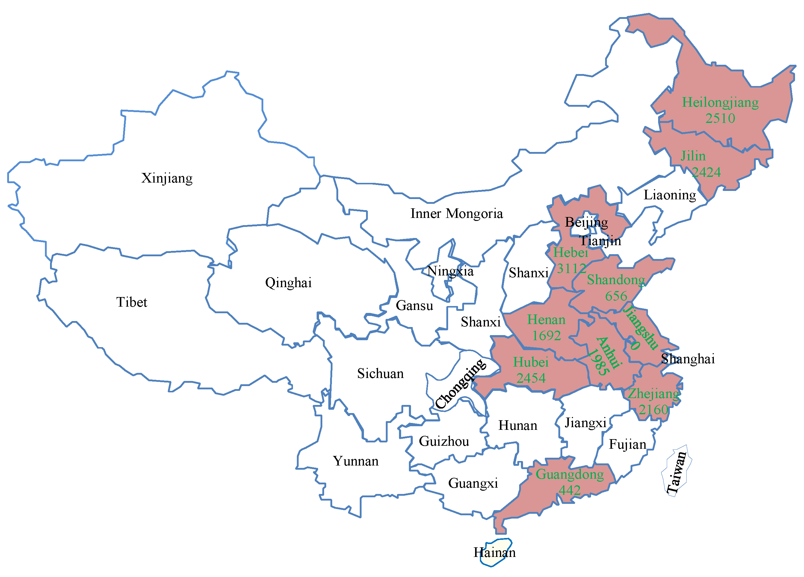
| Province | Difference (Bio), Million RMB | Technology | Location |
|---|---|---|---|
| Jiangsu | 0 | Straw combustion | Southeast |
| Shandong | 656.26 | Straw combustion | East |
| Henan | 1691.97 | Straw combustion | Middle |
| Anhui | 1985.16 | Straw combustion | Southeast |
| Zhejiang | 2159.6 | MSW incineration | Southeast |
| Jilin | 2424.01 | Straw combustion | Northeast |
| Guangdong | 2425.62 | MSW incineration | South |
| Hubei | 2454.01 | Straw combustion | Southeast |
| Heilongjiang | 2510.38 | Straw combustion | North |
| Hebei | 3111.78 | MSW incineration | Middle |
| Province | Biomass industry | Agriculture | ||||
|---|---|---|---|---|---|---|
| PE | TE | AE | PE | TE | AE | |
| Beijing | 21.59 | 0.95 | 20.64 | 205,725.01 | 0 | 205,725.01 |
| Tianjin | 21.42 | 0 | 21.42 | 208,061.32 | 0.19 | 208,061.13 |
| Hebei | 19.33 | 1.44 | 17.89 | 81,235.07 | 3.24 | 81,231.83 |
| Shanxi | 23.37 | 0.07 | 23.3 | 183,566.15 | 1.13 | 183,565.01 |
| Inner Mongolia | 26.56 | 0.28 | 26.29 | 155,857.71 | 1.84 | 155,855.87 |
| Liaoning | 19.71 | 0.56 | 19.15 | 107,759.06 | 1.42 | 107,757.65 |
| Jilin | 15.06 | 1.15 | 13.91 | 145,452.76 | 2.02 | 145,450.74 |
| Heilongjiang | 15.59 | 0.54 | 15.05 | 62,294.32 | 2.35 | 62,291.97 |
| Shanghai | 21.98 | 0 | 21.98 | 203,773.2 | 0 | 203,773.2 |
| Jiangsu | 0 | 0 | 0 | 0 | 0 | 0 |
| Zhejiang | 13.41 | 5.86 | 7.55 | 138,992.58 | 0.87 | 138,991.71 |
| Anhui | 12.33 | 0.95 | 11.38 | 130,149.29 | 3.29 | 130,146.01 |
| Fujian | 19.59 | 2.21 | 17.38 | 115,359.8 | 1.16 | 115,358.64 |
| Jiangxi | 19.68 | 0.09 | 19.59 | 192,359.61 | 1.36 | 192,358.25 |
| Shandong | 4.08 | 2.86 | 1.22 | 26,110.26 | 4.71 | 26,105.55 |
| Henan | 10.51 | 1.05 | 9.46 | 5767.58 | 6.79 | 5760.79 |
| Hubei | 15.24 | 2.17 | 13.07 | 36,496.57 | 3.5 | 36,493.07 |
| Hunan | 21.96 | 0.24 | 21.72 | 38,913.97 | 2.44 | 38,911.53 |
| Guangdong | 15.07 | 5.52 | 9.55 | 43,382.39 | 2.4 | 43,379.98 |
| Guangxi | 24.78 | 0 | 24.78 | 100,572.8 | 2.44 | 100,570.36 |
| Hainan | 22.09 | 0 | 22.09 | 180,474.47 | 0.41 | 180,474.07 |
| Chongqing | 21.73 | 1.12 | 20.61 | 154,210.26 | 0.91 | 154,209.35 |
| Sichuan | 25.15 | 0.27 | 24.88 | 4642.83 | 2.48 | 4640.35 |
| Guizhou | 23.3 | 0 | 23.3 | 166,533.27 | 0.93 | 166,532.34 |
| Yunnan | 27.17 | 0.27 | 26.9 | 127,429.13 | 2.05 | 127,427.08 |
| Xizang | 25.28 | 0 | 25.28 | 220,139.77 | 0 | 220,139.77 |
| Shaanxi | 22.11 | 0.08 | 22.03 | 107,155.97 | 2.35 | 107,153.62 |
| Gansu | 23.46 | 0.17 | 23.3 | 157,124.66 | 0.87 | 157,123.78 |
| Qinghai | 22.83 | 0 | 22.83 | 213,404 | 0 | 213,404 |
| Ningxia | 21.84 | 0 | 21.84 | 207,167.06 | 0.34 | 207,166.72 |
| Xinjiang | 22.77 | 0.01 | 22.76 | 85,353.68 | 1.88 | 85,351.8 |
© 2017 by the authors. Licensee MDPI, Basel, Switzerland. This article is an open access article distributed under the terms and conditions of the Creative Commons Attribution (CC BY) license (http://creativecommons.org/licenses/by/4.0/).
Share and Cite
Yan, Q.; Wan, Y.; Yuan, J.; Yin, J.; Baležentis, T.; Streimikiene, D. Economic and Technical Efficiency of the Biomass Industry in China: A Network Data Envelopment Analysis Model Involving Externalities. Energies 2017, 10, 1418. https://doi.org/10.3390/en10091418
Yan Q, Wan Y, Yuan J, Yin J, Baležentis T, Streimikiene D. Economic and Technical Efficiency of the Biomass Industry in China: A Network Data Envelopment Analysis Model Involving Externalities. Energies. 2017; 10(9):1418. https://doi.org/10.3390/en10091418
Chicago/Turabian StyleYan, Qingyou, Youwei Wan, Jingye Yuan, Jieting Yin, Tomas Baležentis, and Dalia Streimikiene. 2017. "Economic and Technical Efficiency of the Biomass Industry in China: A Network Data Envelopment Analysis Model Involving Externalities" Energies 10, no. 9: 1418. https://doi.org/10.3390/en10091418