Backflow Power Optimization Control for Dual Active Bridge DC-DC Converters


School of Electrical Engineering, Beijing Jiaotong University, Haidian District, Beijing 100044, China
*
Author to whom correspondence should be addressed.
Energies 2017, 10(9), 1403; https://doi.org/10.3390/en10091403
Submission received: 10 August 2017
/
Revised: 2 September 2017
/
Accepted: 6 September 2017
/
Published: 14 September 2017
(This article belongs to the Section F: Electrical Engineering)
Abstract
:This paper proposes optimized control methods for global minimum backflow power based on a triple-phase-shift (TPS) control strategy. Three global optimized methods are derived to minimize the backflow power on the primary side, on the secondary side and on both sides, respectively. Backflow power transmission is just a portion of non-active power transmission in a dual active bridge (DAB) converter. Non-active power transmission time is proposed in this paper, which unifies zero power transmission and backflow power transmission. Based on the proposed index, an optimized control method is derived to achieve both the maximum effective power transmission time and minimum current stress of DAB at the same time. A comparative analysis is performed to show the limitations of the minimum backflow power optimization method. Finally, a prototype is built to verify the effectiveness of our theoretical analysis and the proposed control methods by experimental results.
1. Introduction
In recent years, dual active bridge (DAB) dc-dc converter is an attractive application with the advantages of bidirectional power flow, electrical isolation, high power density, and high transfer efficiency. DAB converter is suitable for the applications in the areas of renewable energy power generation and power electronics applications, such as the battery energy storage systems, and electric vehicles, solid-state transformers [1,2,3,4,5,6].
The traditional single-phase-shift (SPS) control method [2] only uses one degree of freedom of DAB. As a result, SPS control is easy to implement on-chip. However, SPS control only provides high operation efficiency when the voltage conversion ratio d is close to 1. The current stress and current rms for SPS control will increase a lot and the range of soft-switching will decrease when the voltage conversion ratio d is far from 1. Therefore, SPS control is not highly efficient under wide voltage variation conditions.
In order to improve the performance of DAB, various optimization methods have been proposed based on the optimal objectives of current stress and current rms. In [7,8], the extended-phase-shift (EPS) control and the dual-phase-shift control are proposed to reduce the current stress for DAB. Two degrees of freedom are utilized for optimization in EPS and DPS control. In order to obtain the minimum current stress for DAB, the global optimal method for current stress is derived in [9] based on the triple-phase-shift (TPS) control method. Similar to the optimized methods for current stress, a numerical method is used to find the optimal control parameters for minimum rms of transformer current in [10]. In [11,12], the analytical expressions of the optimal control parameters are derived for minimum rms of transformer current. As a result, the optimal control method can be implemented by on-line and on-chip calculation. These optimal methods above all take the current as the optimal objectives for DAB.
In addition to current, many other optimal objectives also have been studied in the existing literature. Like the definition of reactive power in sinusoidal ac circuit, the reactive power is defined and minimized for a DAB converter in [13,14,15]. However, it is too complex to obtain the analytical expressions of the control parameters based on the optimal objective of reactive power. Only numerical solutions can be found for the optimal objective of reactive power in [13,14,15]. Furthermore, the physical significance for the reactive power in DAB is not clear enough. Therefore, this kind of optimal method has low practicability.
Minimization of backflow power is another common optimal objective for DAB. The delivery direction of backflow power is contrary to the delivery direction of average power transmission in DAB. Thus, the backflow power indeed reduces the power transmission efficiency in DAB. In [16,17], a novel extended-single-phase shift (ESPS) control method and an easy-to-implement control method are proposed, respectively. These two control methods can eliminate (to zero) the backflow power on both sides of the DAB converter. However, these two references do not take all operation modes of DAB into consideration and no global optimal results are derived for the whole load range. As a result, these two control methods are just local optimal results and they can only be implemented under light and medium load range conditions. Reference [18] derives the dual-phase-shift control method to eliminate the backflow power in the input side of DAB. Reference [19] proposes a zero circulating current (ZCC) control method to eliminate the backflow power on the output side of DAB. These two control methods only use two degrees of freedom for optimization of backflow power, leading to local optimal results rather than global optimal results. Moreover, these two control methods eliminate the backflow power just on one side of DAB and the backflow power on both sides cannot be optimized at the same time. In [20], the sum of backflow power on both sides is minimized, so the backflow power on both sides can be reduced at the same time, however, the optimized control parameters are derived just when the voltage conversion ratio is equal to 1. Therefore, no global and complete control methods for backflow power are derived in existing research. Furthermore, the optimization performance of various optimized objectives of backflow power mentioned above (i.e., the backflow power on the primary side, the secondary side and on both sides) have not been compared to each other.
In [21,22], the circulating current is defined as the transformer current during the period of time when no active power is transmitted on the output side of DAB. In [22], the circulating current is the transformer current during the period of time when backflow power and zero power (caused by vcd = 0) are transmitted on the output side of DAB. The optimal objective in [21,22] is to minimize the rms value of circulating current. Only the circulating current on the output side is considered in [21,22]. In [23], the concept of non-active power which is proposed in [24] is utilized to define a new optimization objective, i.e., non-active power loss. In [24], the non-active current is defined just for the SPS control method to be the result of backflow power transmission. However, the non-active current caused by zero power transmission is not considered in [23,24]. Similar to the optimized methods in [7,8,9,10,11,12], these optimized control methods in [21,22,23,24] are essentially still for current. In fact, the backflow power is just a portion of the non-active power transmission in DAB and the limitations of the backflow power control method are not presented. The complete non-active power transmission in DAB is supposed to be defined for the performance optimization.
Firstly, this paper proposes optimized control methods for global minimum backflow power based on triple-phase-shift (TPS) control strategy. Three global optimized methods are derived to minimize the backflow power on the primary side, on the secondary side and on both sides, respectively. Compared to the existing backflow power optimization methods in the published literature, the backflow power is minimized by the three proposed control methods. A comparative analysis is carried out to evaluate the performance differences among these three control methods and SPS control. The comparative analysis results show however that the power transmission efficiency may not be improved in some cases by the backflow power optimization methods. Therefore, the concept of maximum non-active power transmission time is proposed in this paper and it unifies the zero power transmission and the backflow power transmission together. Then, a new optimal objective is defined as the maximization of the effective power transmission time ratio in the DAB converter. The derived optimized control method achieves both the maximum effective power transmission time and minimum current stress of DAB at the same time. A comparative analysis is performed to show that the minimum non-active power optimization method has the best optimization performance and also explain the limitations of the minimum backflow power optimization method. Finally, a prototype is built to verify the effectiveness of the theoretical analysis and the proposed control methods by experimental results.
2. Operation Principles
2.1. DAB Converter
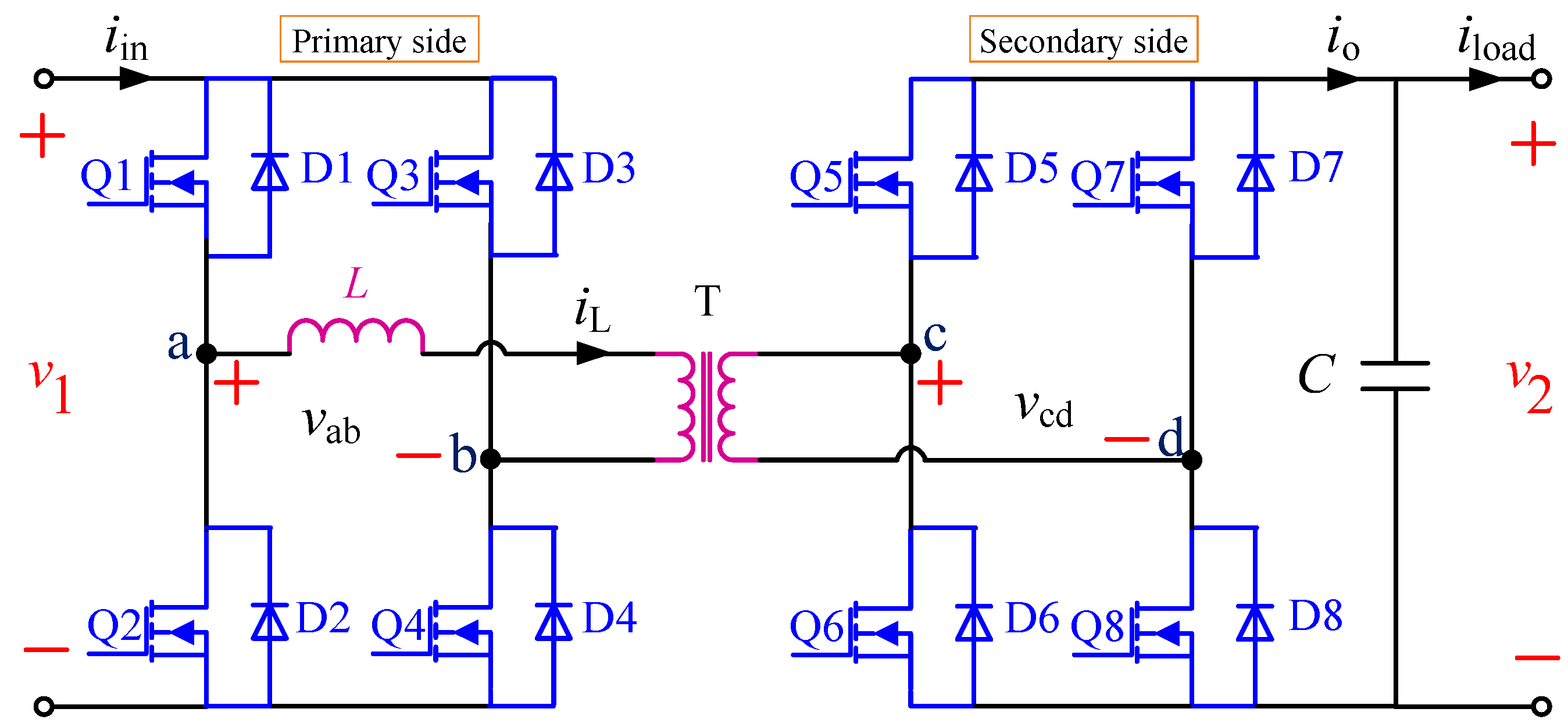
The DAB converter is shown in Figure 1. A high-frequency transformer T connects the primary H-bridge (Q1 to Q4) and the secondary H-bridge (Q5 to Q8). The inductance L is the value which has been reflected to the primary side. L includes the leakage inductance of transformer T and the additional complementary inductance. V1 is the dc-bus voltage on the primary side (input voltage). V2 is the dc-bus voltage on the secondary side (output voltage), respectively. The turns ratio n is set to 1 to simplify the analysis process. The electric quantities on the secondary side can be reflected to the primary side when n ≠ 1. As a result, the analysis process is similar to the situation when n = 1.
2.2. Selected Operating Modes of Triple Phase Shift Control
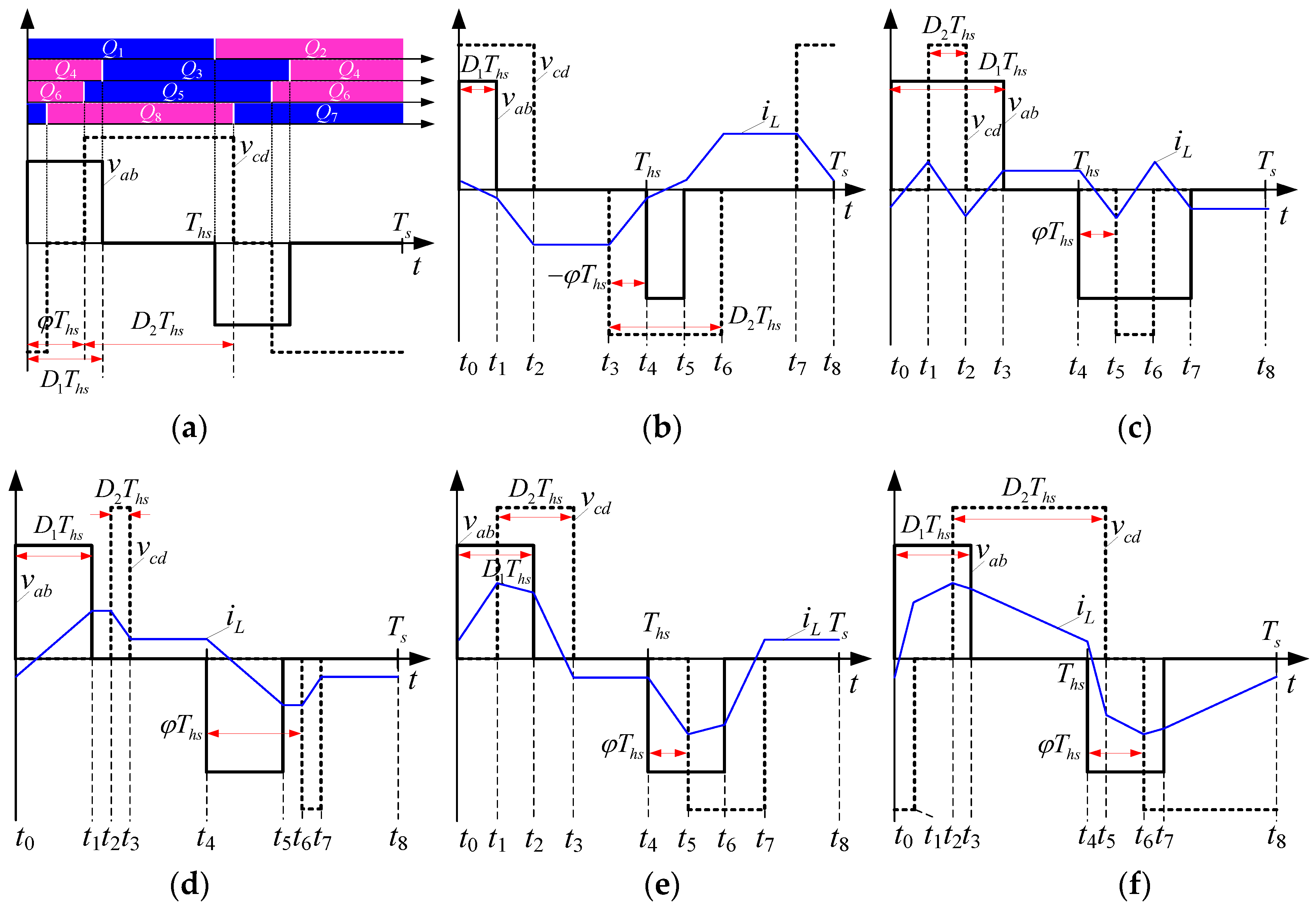
Due to the symmetry of DAB, the analysis based on positive power flow is enough, and analysis methods are similar to the situation when negative power flow is engaged. In [25], the operating modes of TPS are divided into twelve types. Only eight operating modes have the ability for positive power transmission, as presented in [25].The mode 1 and mode 1′ in [25] have the same transmission power capability. However, the backflow power in mode 1′ is apparently larger than mode 1 due to the opposite polarity between vab and vcd in mode 1′. It means that the power cannot be transferred from the primary side to the secondary side and from the secondary side to the load side at the same time in mode 1′. Similar conclusions can be drawn for mode 2′ and mode 4, respectively. The backflow power in mode 2′ is obviously larger than in mode 2, while the backflow power in mode 4 is obviously larger than in mode 5. The rest of the operating modes in [25], i.e., mode 3′, mode 4′, mode 5′, and mode 6′, can only transfer negative power. As a result, only five types of operating modes are selected to achieve both positive transmission power from the primary side to the secondary side and small backflow power. These five modes are depicted in Figure 2. Based on these five modes, an optimized control strategy could be derived in Section 3 to minimize the backflow power in a DAB converter when the transmission power is positive.
In Figure 2a, φ is defined as the outer phase shift ratio between the drive signals of Q1 (or Q2) and Q5 (or Q6). When the drive signal of Q1 is ahead of Q5, φ is positive. Otherwise, when the drive signal of Q1 lags behind Q5, φ is negative. D1 is defined as the inner phase shift ratio in the primary H-bridge between the drive signals of Q1 (or Q2) and Q3 (or Q4). D2 is defined as the inner phase shift ratio in the secondary H-bridge between the drive signals of Q5 (or Q6) and Q7 (or Q8). The operation constraints and transmission power of these five modes are listed in Table 1. K is denoted as the normalized transmission power to the reference value AV1V2, i.e., k = PDAB/(AV1V2). A is the constant coefficient Ths/(2L).The voltage conversion ratio d is defined as d = V2/V1. The maximum transmission power of DAB is k = 0.5 when D1 = 1, D2 = 1 and φ = 0.5. As shown in Figure 2, understeady-state conditions, the waveforms of vab, vcd and iL are symmetric in an adjacent half switching period. Therefore, the following mathematical analysis is carried out only in half a switching period for simplification.
3. Global Minimum Backflow Power Control
3.1. Backflow Power Under SPS Control
Figure 3 shows the operation waveforms of DAB under a single-phase-shift (SPS) control strategy. The phase shift time between the voltage vab and vcd is defined as φ∙Ths, where Ths is a half switching period. The phase shift ratio between vab and vcd is φ. iin and io are the input current on the primary side and the output current on the secondary side, respectively.
For simplification, only the positive power flow from the primary side to the secondary side is analyzed in this paper. As can be seen in Figure 3, the transmission power of DAB flows back to the primary side (i.e., power supply) from the DAB during t0 to t01′ and t2 to t23′ while the transmission power of the DAB flows back to the DAB from the load side during t01′ to t1 and t23′ to t3. The transmission power during these periods is defined in this paper as the backflow power. Backflow power is one type of the non-active power in DAB and it will reduce the power transmission efficiency in DAB. In Figure 3, the backflow power on the primary side and secondary side are defined by Equations (1) and (2), respectively.
where both Qp and Qs are positive values.
3.2. Minimum Backflow Power Conrtrol (MBPC) at Low Power Level
Mode 1 to mode 4 in Figure 2 are the operating modes at low power level. Moreover, both the backflow power on the primary side (i.e., Qp) and these secondary side (i.e., Qs) can be eliminated simultaneously to zero in mode 1 to mode 4. Therefore, these modes have the minimum backflow power on both sides. Optimized control parameters in each operating mode can be derived as below based on the optimal object Qp = Qs = 0.
MBPC in mode 1. In order to eliminate Qp and Qs, the current conditions iL(t0) ≥ 0, iL(t1) ≥ 0, iL(t2) = 0 and iL(t3) = 0 should be satisfied to obtain:
Substituting Equation (3) into the expression of transmission power in Table 1, the optimized control parameters with its constraints in mode 1 can be solved:
Based on the constraints of mode 1 in Table 1, the maximum transmission power is:
MBPC in mode 2. Solving the current conditions iL(t0) = 0, iL(t1) ≥ 0, iL(t2) ≥ 0 and iL(t3) = 0 for the elimination of Qp and Qs we obtain:
Substituting Equation (6) into the expression of transmission power in Table 1, the optimized control parameters with its constraints in mode 2 can be solved:
According to the constraints of mode 2 in Table 1, the maximum transmission power is:
MBPC in mode 3. Solving the current conditions iL(t0) = 0, iL(t1) ≥ 0, iL(t2) ≥ 0 and iL(t3) = 0 for the elimination of Qp and Qs we can obtain:
This indicates that the elimination of backflow power in mode 3 is only determined by D1 and D2. The outer phase shift ratio φ has no effect on it. However, in order to reduce the root-mean-square (RMS) current of iL as much as possible, φ is supposed to be D1 in this mode. Therefore, the period of time t1 to t2 can be eliminated to zero and RMS current can be reduced, as shown in Figure 2d.
Substituting Equation (9) into the expression of transmission power in Table 1, the optimized control parameters of mode 3 can be calculated:
The maximum transmission power in mode 3 is:
MBPC in mode 4. Solve the current conditions iL(t0) = 0, iL(t1) ≥ 0, iL(t2) ≥ 0 and iL(t3) = 0 to eliminate Qp and Qs:
Substituting Equation (12) into the expression of transmission power in Table 1 to obtain:
According to the quadratic curving relationship in Equation (13), it can be obtained that:
Therefore, the maximum transmission power in mode 4 is:
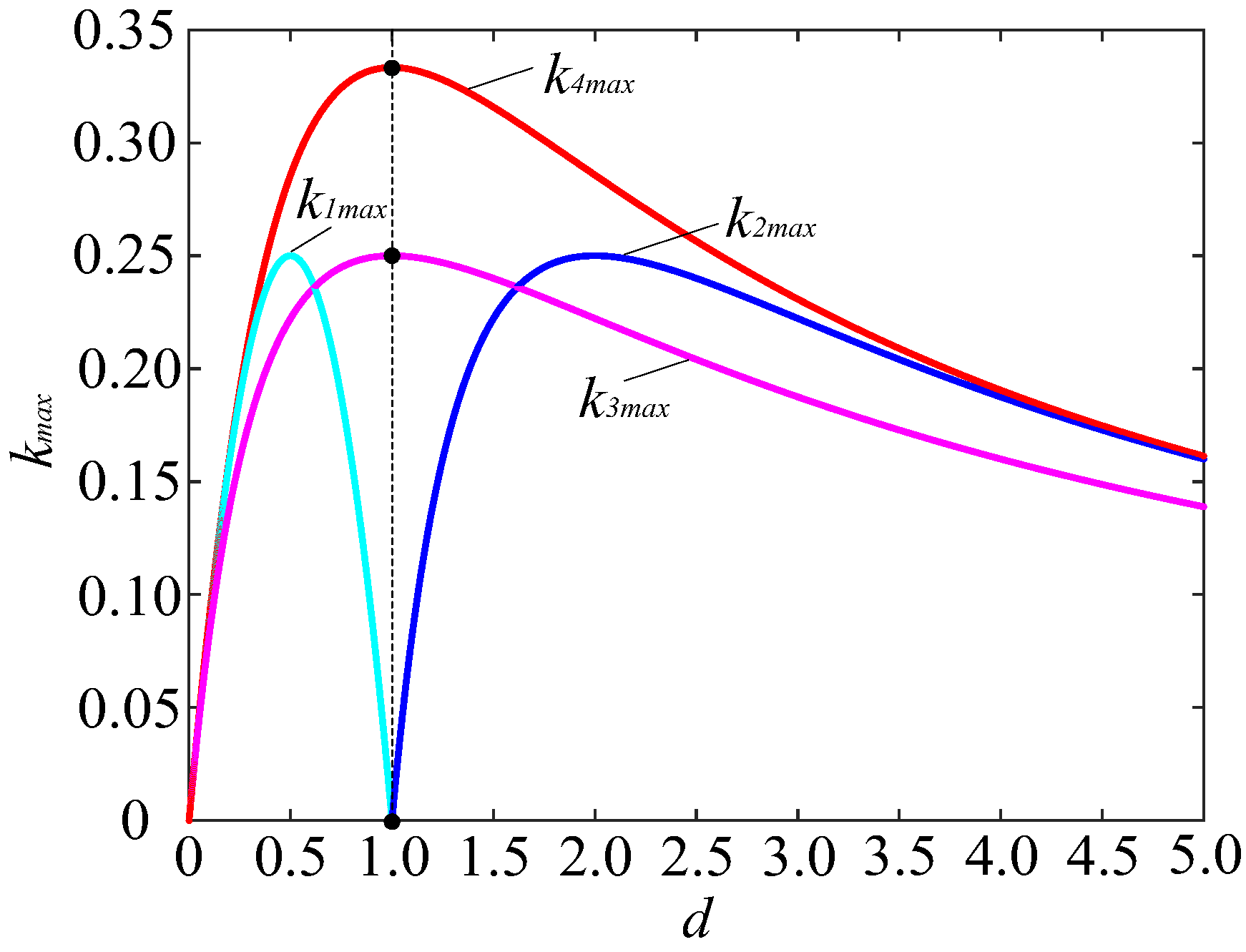
Figure 4 presents the curves of kmax versus d for mode 1 to mode 4 according to Equations (5), (8), (11) and (15). From Figure 4, we can conclude that k4max is larger than the other three modes under different d. Especially when d is equal to 1, mode 1 and mode 2 will not be effective anymore while k4max reaches its maximum value. This indicates that mode 4 has the widest power range for zero backflow power on both the primary side and secondary side. As a result, mode 4 is the optimized operating mode at low power level.
Similar to the backflow power in mode 3, the elimination of backflow power in mode 4 is only dependent on D1 and D2. The outer phase shift ratio φ has no effect on it. For simplicity, φ is designed to be a linear relationship with D1 or D2 as shown below:
The optimized control parameters of mode 4 can be solved as:
3.3. Minimum Backflow Power Conrtrol at Medium Power Level
If the transmission power exceeds k4max, the DAB converter will operate in mode 5. However, Qp and Qs cannot be eliminated at the same time in mode 5 when k is larger than k4max. Mode 5 can be further subdivided into five operating modes based on the current conditions of iL. Due to the symmetry of vab, vcd and iL in the adjacent half switching period, only the current values in a half period are presented:
- (1)
- Mode 5A. When iL(t0) ≥ 0, iL(t1) ≥ 0, iL(t2) ≥ 0, and iL(t3) ≥ 0, Qp can be eliminated to zero, while Qs cannot be eliminated, as shown in Figure 5a.
- (2)
- Mode 5B. When iL(t0) < 0, iL(t1) ≤ 0, iL(t2) ≥ 0, and iL(t3) ≥ 0, Qs can be eliminated to zero, while Qp cannot be eliminated, as shown in Figure 5b.
- (3)
- Mode 5C. When iL(t0) ≤ 0, iL(t1) ≥ 0, iL(t2) ≥ 0, both Qp and Qs cannot be eliminated to zero. However, it is the only operating mode to reach the maximum transmission power of DAB, i.e., k = 0.5 when D1 = 1, D2 = 1 and φ = 0.5, as shown in Figure 5c.
- (4)
- Mode 5D. When iL(t0) ≥ 0, iL(t1) ≥ 0, iL(t2) ≥ 0, and iL(t3) ≤ 0, both Qp and Qs are larger than that in mode 5A under certain k. Therefore, this mode is not selected to be optimized below.
- (5)
- Mode 5E. When iL(t0) ≤ 0, iL(t1) ≤ 0, iL(t2)≤ 0, and iL(t3) ≥ 0, both Qp and Qs are larger than that in mode 5B under certain k. Therefore, this mode is also not selected to be optimized below.
As analyzed above, only mode 5A, mode 5B and mode 5C are selected to be optimized as below. There are two common optimal objectives in mode 5, i.e., Qp = 0 or Qs = 0, to eliminate the backflow power on the primary side and secondary side, respectively. Based on the two objectives, only two control degrees of freedom are considered in [18,19].
In this section, the two optimized objectives are modified to obtain a smaller backflow power on both sides with three control degrees of freedom. The optimized control parameters at medium power level are derived based on two modified objectives respectively as below:
Objective 1: The objective 1 at medium power level is to eliminate the primary backflow power Qp with minimum secondary backflow power Qs:
The optimized objective in Equation (18) not only achieves zero backflow on the primary side, but also gives consideration to the reduction of backflow power on the secondary side. Moreover, when iL(t0), iL(t1), iL(t2), and iL(t3) are not smaller than zero, Qp can be eliminated to zero. Therefore, the optimized mode for objective 1 is mode 5A, as shown in Figure 5a. The secondary backflow power Qs in this case is:
where A is the constant coefficient Ths/(2L).
It can be seen from Equation (19) that Qs cannot be eliminated to zero when Qp is zero. However, the value of Qs can still be minimized based on appropriate control parameters. According to Equations (18), (19) and the transmission power in Table 1, the optimized control parameters are derived in Equation (20) (the detailed derivation process is presented in Appendix A).
The optimized results indicate that the value of iL(t0) is exactly equal to zero. That is to say, the optimized control parameters in Equation (20) are actually located at the boundary of mode 5A and mode 5C. The maximum transmission power is reached when α1 in Equation (20) is equal to zero:
Objective 2: The objective 2 at medium power level is to eliminate the secondary backflow power Qs with minimum primary backflow power Qp
As long as the current conditions iL(t0) ≤ 0, iL(t1) ≤ 0, iL(t2) ≥ 0, and iL(t3) ≥ 0 are met, Qs can be eliminated to zero, as shown in Figure 5b. The primary backflow power Qp in this case is:
It can be seen from Equation (23) that Qp cannot be eliminated to zero when Qs is zero. However, the value of Qs can still be minimized based on appropriate control parameters. Based on Equations (22), (23) and the transmission power in Table 1, the optimized control parameters can be derived as below:
Under the optimized control parameters in Equation (24), the value of iL(t1) is exactly equal to zero. Therefore, the optimized control method by in Equation (24) is actually located at the boundary of mode 5B and mode 5C.
The maximum transmission power is reached when α2 in Equation (24) is equal to zero:
3.4. Minimum Backflow Power Conrtrol at High Power Level
Along with the increase of transmission power, k will exceed k5Amax or k5Bmax. In this case, the current value of iL(t0) is smaller than zero while the current value of iL(t1) is larger than zero. The DAB converter will operate in mode 5C, as shown in Figure 5c. The backflow power on both sides needs to be recalculated by Equations (26) and (27):
Objective 1: Objective 1 at high power level is to eliminate the primary backflow power Qp:
Substituting the expression of transmission power in Table 1 into Equation (26) to eliminate the variable φ, the optimized control parameters can be derived:
Objective 2: Objective 2 at high power level is to eliminate the secondary backflow power Qs:
Similarly, the optimized control parameters can be derived as:
As can be seen in Equations (28) to (31), whether objective 1 or objective 2 is selected to be optimized, three control degrees of freedom are needed. It indicates that only single-side backflow power (i.e., Qp or Qs) can be optimized at high power level.
Equations (17), (20) and (29) constitute the “global minimum primary backflow power control method (GMPBPC)”, while the Equations (17), (24) and (31) constitute the “global minimum secondary backflow power control method (GMSBPC)”.
3.5. Comparative Analysis of Global Minimum Backflow Power Control
3.5.1. Backflow Power
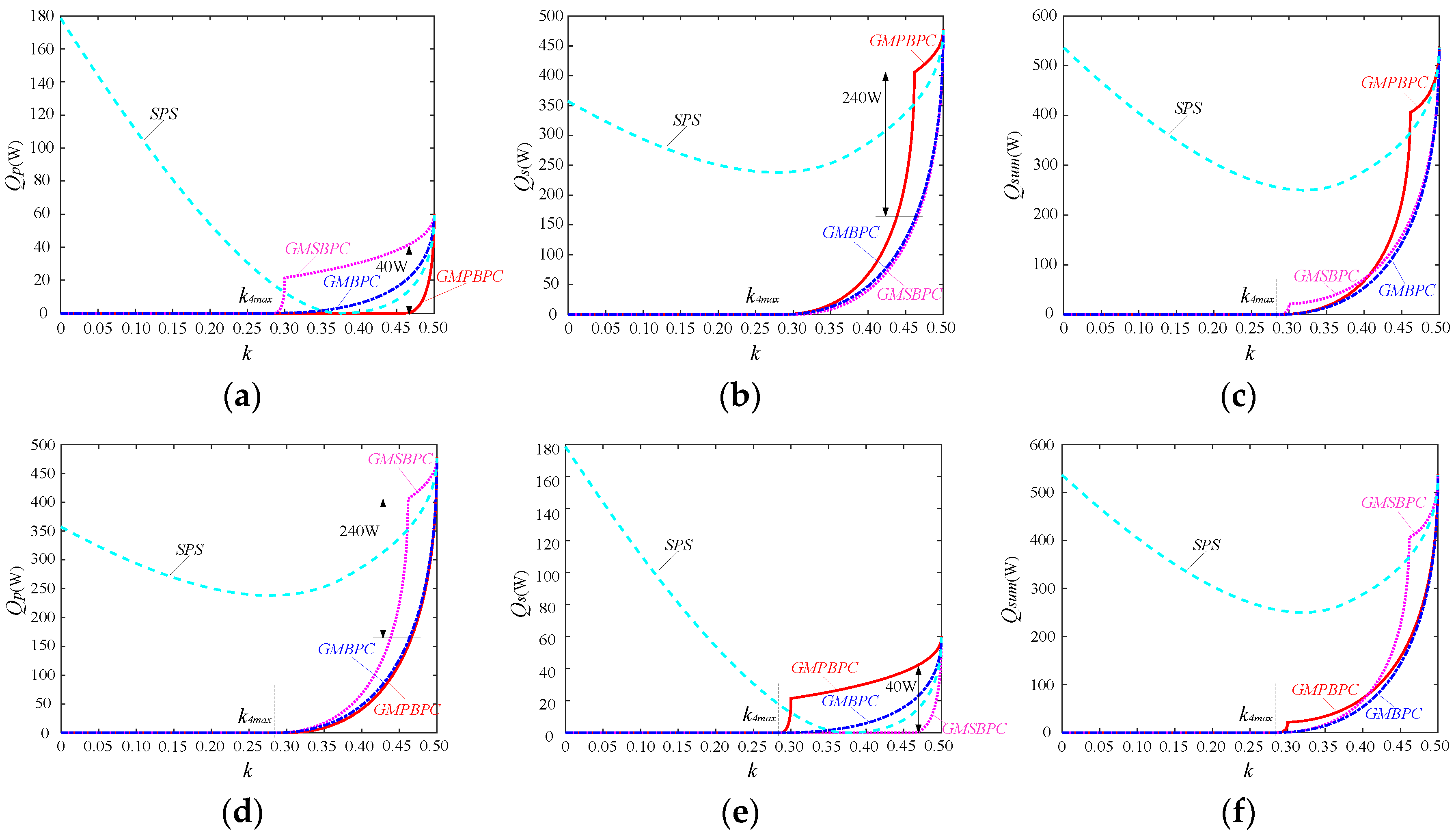
The backflow power of GMPBPC, GMSBPC and the traditional SPS control method are depicted in Figure 6. It can be seen in Figure 6a,b that GMPBPC and GMSBPC achieve minimum Qp and minimum Qs, respectively, as expected. Compared to the SPS control method, these two optimized methods can reduce backflow power effectively, especially at lower power level. However, at higher power level, the backflow power of optimized methods may be even larger than the backflow power of the SPS control method.
Under the condition when d = 2 (V1 = 60 V, V2 = 120 V), Qs of GMPBPC is much larger than Qs of other methods at higher power level. The maximum difference of Qs between GMPBPC and GMSBPC is about 240 W, as shown in Figure 6b. However, the maximum difference of Qp between GMSBPC and GMPBPC is only about 40 W, as shown in Figure 6a. As a result, GMPBPC has worse optimized results in comparison to GMSBPC when d is larger than 1. Similarly, GMSBPC has worse optimized results in comparison to GMPBPC when d is smaller than 1, as shown in Figure 6d,e.
As analyzed above, the control method should be switched to GMPBPC when d is larger than 1 and switched to GMSBPC when d is smaller than 1, in order to ensure good optimized performance of DAB under different voltage conversion ratio d. However, the mode switching increases the complexity of the implementation in digital controller.
In order to optimize the backflow power in both sides under arbitrary voltage conversion ratio d but without mode switching, an alternative optimal objective is to minimize the sum of backflow power in both sides as below.
Objective 3: The objective 3 is to minimize the sum of primary and secondary backflow power, i.e., Qsum:
At low power level, the optimized control parameters has been derived in Section 3.2, i.e., mode 4, and Qsum is reduced to zero. At medium power level, Equations (18) and (22) are essentially equivalent to the optimal objectives “minimum Qsum” in mode 5A and mode 5B, respectively. The optimized results are located at the boundary of mode 5C. At high power level, only mode 5C has the ability to reach the maximum power transmission of DAB. As a consequence, the global minimum Qsum can only be derived in mode 5C when transmission power k is larger than k4max. The optimized control parameters are derived based on Equations (26), (27) and (32) as shown below:
The control method which consists of Equations (17) and (33), is called as “global minimum backflow power control (GMBPC)” in this paper.
As can be seen in Figure 6a,b, the values of Qp and Qs in GMBPC are always between the values in GMPBPC and GMSBPC. It indicates that the optimal objective in Equation (32) is essentially a tradeoff between minimum Qp and minimum Qs. Moreover, as shown in Figure 6b, the optimized results of GMBPC are closer to the optimized results of GMSBPC when d = 2. This is because Qs accounts for the largest portion of Qsum (i.e., Qs >> Qp) at higher power level when d = 2, GMBPC is prone to reduce Qs when d is larger than 1. Figure 6d–f show Qp, Qs, and Qsum at d = 0.5 (V1 = 120 V, V2 = 60 V) respectively. The optimized results in Figure 6d–f show the symmetry with respect to the optimized results when d = 2 (V1 = 60 V, V2 = 120 V) in Figure 6a–c. Therefore, GMBPC is prone to reduce Qp when d is smaller than 1. As a result, the optimized performance of GMBPC is similar to the optimized performance of mode switching between GMPBPC and GMSBPC. The mode switching can be avoided.
In conclusion, GMBPC not only has nearly the same optimized performance as GMPBPC when d is smaller than 1 or as GMSBPC when d is larger than 1 without mode switching, but also has smaller Qsum than other methods. Therefore, GMBPC is supposed to have better performance than other two optimized methods. The optimized control parameters and the power range of the three derived methods above are listed in Table 2.
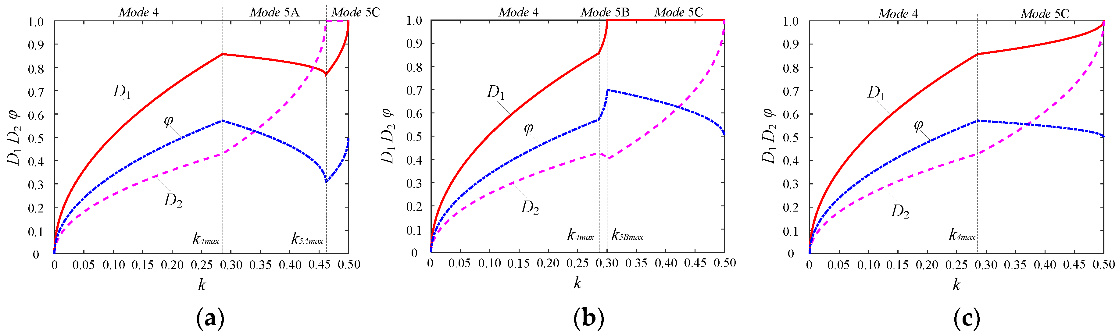
3.5.2. Control Parameters
According to Table 2, the optimized control parameters D1, D2, and φ versus k are depicted in Figure 7 when d = 2 (V1 = 60 V, V2 = 120 V). As can be seen in Figure 7, the control parameters of all these three control methods are piecewise continuous function of k. Only two subsections (i.e., low and high power level) exist in GMBPC, while three subsections (i.e., low, medium and high power level) are in GMPBPC and GMSBPC. Moreover, D1 and D2 change monotonically in GMBPC. Therefore, GMBPC is easier to be implemented compared to other two methods.
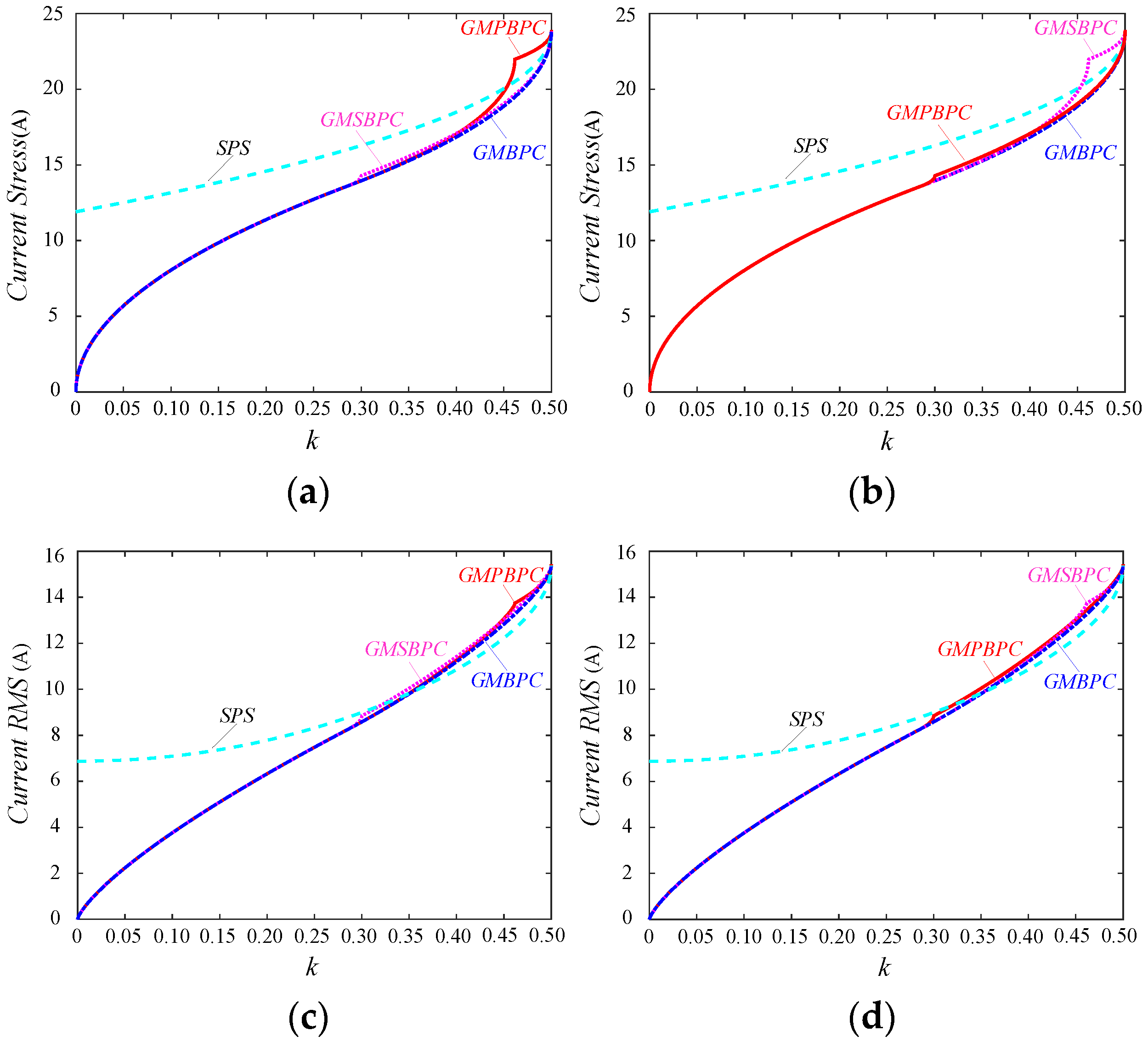
3.5.3. Current Stress and Current rms
In order to further study the performance differences of the three optimized methods, the current stress and the current rms value of iL are compared in Figure 8. Compared to the traditional SPS control method, the current stress and current rms can be reduced effectively by all the three optimized methods especially at lower power level. However, as shown in Figure 8a, the current stress of GMPBPC becomes larger than with other control methods (even than SPS control method) at higher power level when d is larger than 1. Similar situations can also be seen in Figure 8b where the current stress of GMSBPC becomes larger than other methods when d is smaller than 1. A similar phenomenon has been seen and analyzed in Figure 6 in regard to backflow power Qp and Qs. As a result, the same conclusion can be drawn that GMPBPC has worse performance when d is larger than 1 while GMSBPC has worse performance when d is smaller than 1.
As shown in Figure 8c,d, the differences of current rms are smaller than the differences of current stress among the three optimized methods. However, current rms of the three optimized methods all becomes slightly larger than with the SPS control method at higher power level, which means larger conduction losses arise in a higher power operation range by the optimized methods.
In general, GMBPC has the best current performance compared to the other two optimized control methods.
3.5.4. Switching Characteristics
Neglecting the resonance process during switching transition, the soft-switching is generally determined by the polarity of the current at the switching moment. At low power level, all the optimized methods operate in mode 4 and the current satisfies the condition when iL(t0) = 0, iL(t1) ≥ 0, iL(t2) ≥ 0 and iL(t3) = 0. Therefore, Q3, Q4, Q5 and Q6 are turned on at zero-voltage-switching (ZVS) while Q1, Q2, Q7 and Q8 are turned off at zero-current-switching (ZCS) in mode 4. All the switching devices can achieve soft-switching at low power level.
At medium power level, the GMPBPC method requires that iL(t0) = 0, iL(t1) > 0, iL(t2) > 0 and iL(t3) > 0. Therefore, Q3, Q4, Q5, Q6, Q7 and Q8 are turned on at ZVS while Q1 and Q2 are turned off at ZCS in mode 5. Similarly, Q1, Q2, Q3, Q4, Q5 and Q6 are turned on at ZVS while Q7 and Q8 are turned off at ZCS in mode 5 for the GMSBPC method. Thus, all the switching devices can achieve soft-switching at medium power level.
At high power level, all three optimized control methods operate in mode 5C under the conditions when iL(t0) < 0, iL(t1) > 0, iL(t2) > 0 and iL(t3) > 0. As a result, all the switching devices can be turned on at ZVS at high power level.
In conclusion, based on the comparative analysis above, GMBPC is a preferable choice to be a tradeoff between min Qp by GMPBPC and min Qs by GMSBPC. Compared to GMPBPC and GMSBPC, GMBPC allows smaller current stress, smaller current rms value, easier implementation method and wider ZVS range.
4. Non-Active Power Transmission in DAB Converter
4.1. Non-Active Power Transmission Time in DAB Converter
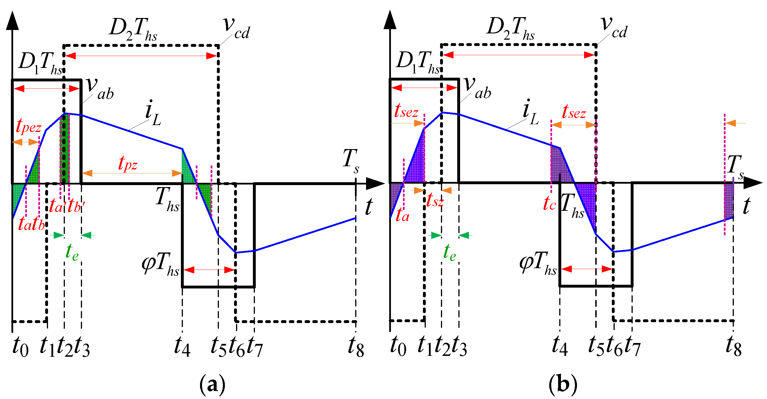
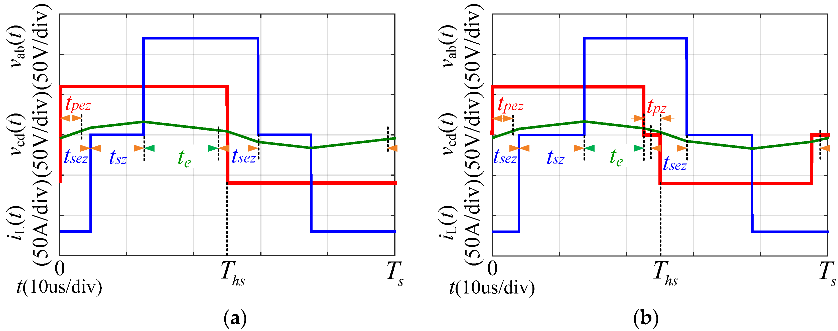
The global minimum backflow power optimization methods are derived in Section 3. However, the backflow power transmission is just a portion of the non-active power transmission in a DAB converter. The ideal maximum power transmission efficiency in DAB occurs when positive power is transmitted from the primary side to the secondary side while positive power is also transmitted from the secondary side to the load side at the same time, e.g., the period of t2 to t3 in Figure 9. However, as shown in Figure 9a, the practical situation on the primary side of DAB is that transmission power flows back to the primary side during t0 to ta and transmission power is zero on the primary side during t3 to t4. Therefore, non-active power transmission time on the primary side contains two portions during t0 to ta (i.e., the backflow power) and t3 to t4 (i.e., the zero power) respectively. A similar situation can also be seen on the secondary side of the DAB, as shown in Figure 9b.
However, the factor of zero power transmission is not considered in Section 3 with the optimal objective of backflow power. Although backflow power is minimized by the methods derived in Section 3, the time of zero power transmission may increase. As a result, the power transmission efficiency may not be improved by the optimization of backflow power.
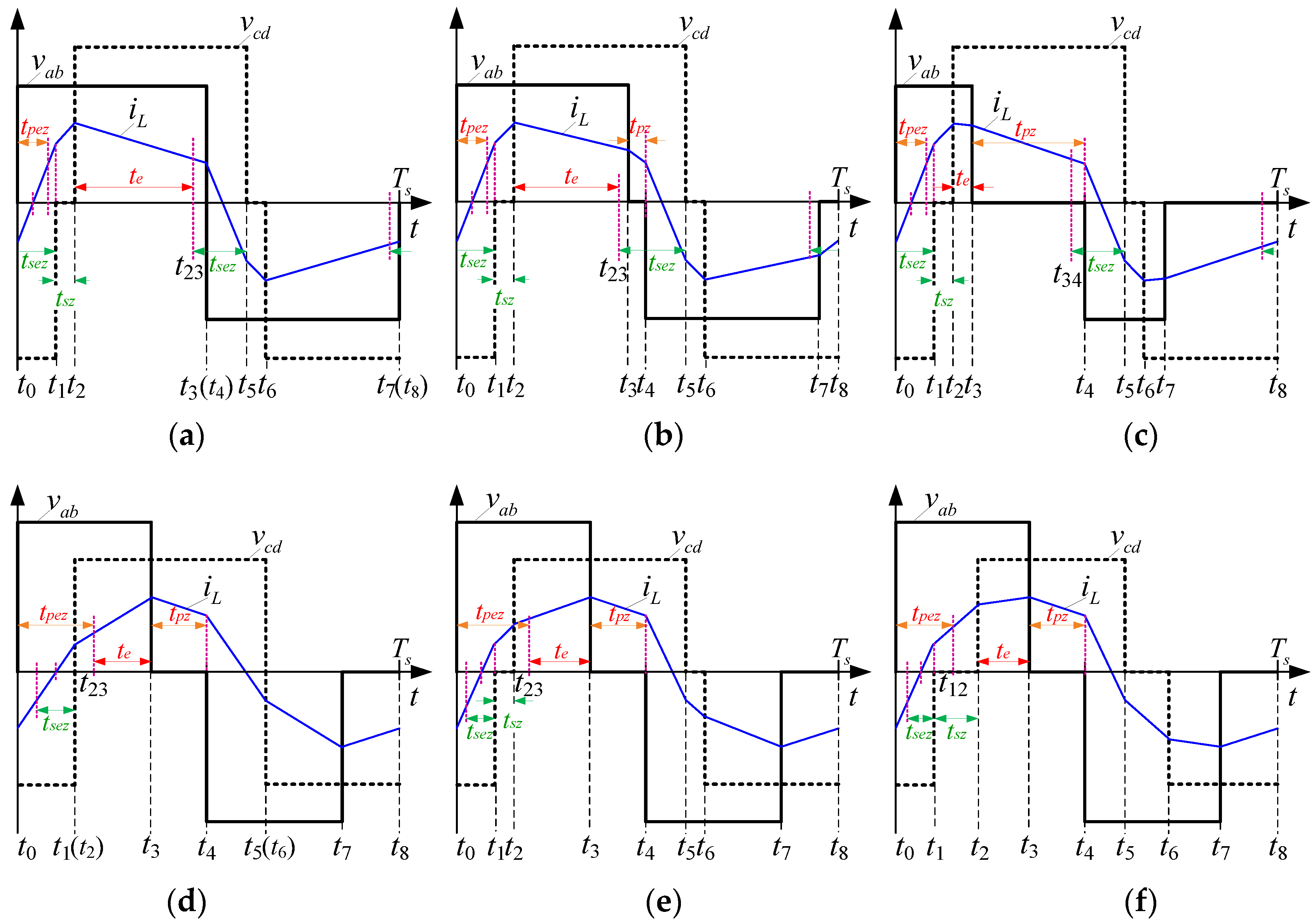
In order to optimize the non-active power transmission in DAB, the concept of maximum non-active power transmission time is proposed in this section. Taking the operation mode in Figure 9 as an example, zero power transmission on the primary side occurs during t3 to t4. The duration of t3 to t4 is denoted as tpz. The backflow power Qp is transmitted back to the primary side during t0 to ta. The same amount of power which is also equal to Qp, can be transmitted from the primary side to the secondary side during ta to tb. Therefore, the average power during t0 to tb is zero. The period of t0 to tb can be called the equivalent zero power transmission time, just like the zero power transmission during t3 to t4. However, the same amount of power which is equal to Qp, can also be transmitted from the primary side to the secondary side during other different time intervals, e.g., during ta′ to tb′ in Figure 9a. The duration of ta to tb is longer than the duration of ta′ to tb′ due to the smaller average current during ta to tb. Therefore, t0 to tb is the maximum equivalent zero power transmission time on the primary side caused by backflow power Qp. The duration of t0 to tb is denoted as tpez. As a consequence, the maximum non-active power transmission time on the primary side, i.e., tpna, can be defined to be the sum of tpz and tpez as given below:
The non-active power transmission time ratio (NTR) on the primary side is defined as γp. γp is the percentage of tpna to Ths. Therefore, the effective power transmission time ratio (ETR) on the primary side can be defined as δp = 1 − γp:
Similarly, as shown in Figure 9b, the non-active power transmission time ratio on the secondary side, i.e., γs, is the percentage of tsna to Ths. The ETR on the secondary side can be defined as δs = 1 − γs. Nonactive power transmission time unifies the zero power transmission and the backflow power transmission together. The backflow power is converted to zero power transmission time equivalently. Therefore, δp indicates the active power transmission time efficiency on the primary side while δs indicates the active power transmission time efficiency on the secondary side. The active power transmission time efficiency for DAB is limited by the minimum transmission time efficiency either on the primary side δp or on the secondary side δs, i.e., min (δp, δs). As a result, the active power transmission time efficiency for a DAB converter on both sides cannot be just denoted as the tradeoff between δp and δs, e.g., the summation of δp and δs.
The effective power transmission time te for a DAB converter can be denoted as the time during which no non-active power on the primary side or on the secondary side is transmitted. In Figure 9, the period of t2 to t3 is the effective power transmission time. Therefore, it makes sense for te to indicate the power transmission time efficiency for DAB. For the purpose of minimizing the non-active power transmission time on both sides for DAB, a new optimal objective can be constructed in Equation (36) to maximize the effective power transmission time ratio (δe = te/Ths):
max δe
4.2. Minimum Non-Active Power Transmission Time Control (MNPC) at Low Power Level
At low power level, GMPBPC, GMSBPC and GMBPC are all in mode 4 with the control parameters shown in Table 2. The time tpna, tsna and te can be calculated as:
In this case, when D1 and D2 are selected to be their maximum values, γp and γs can be minimized. Moreover, as can be seen in Equation (37), the optimal objective “max δe” is equivalent to the objectives “min γp” and “min γs” at the same time. Therefore, the effective power transmission time te can be maximized while the non-active power transmission time can be minimized in the meantime. The maximum values of D1 and D2 can be obtained based on the limitation condition of φ in Equation (12). Optimized results show that the MNPC method in mode 4 is located at the boundary of mode 1 and mode 4 when d < 1 or the boundary of mode 2 and mode 4 when d > 1. Moreover, it can be demonstrated that the control parameters of MNPC in mode 1 and mode 2 are the same as the results in Equations (4) and (7), respectively.
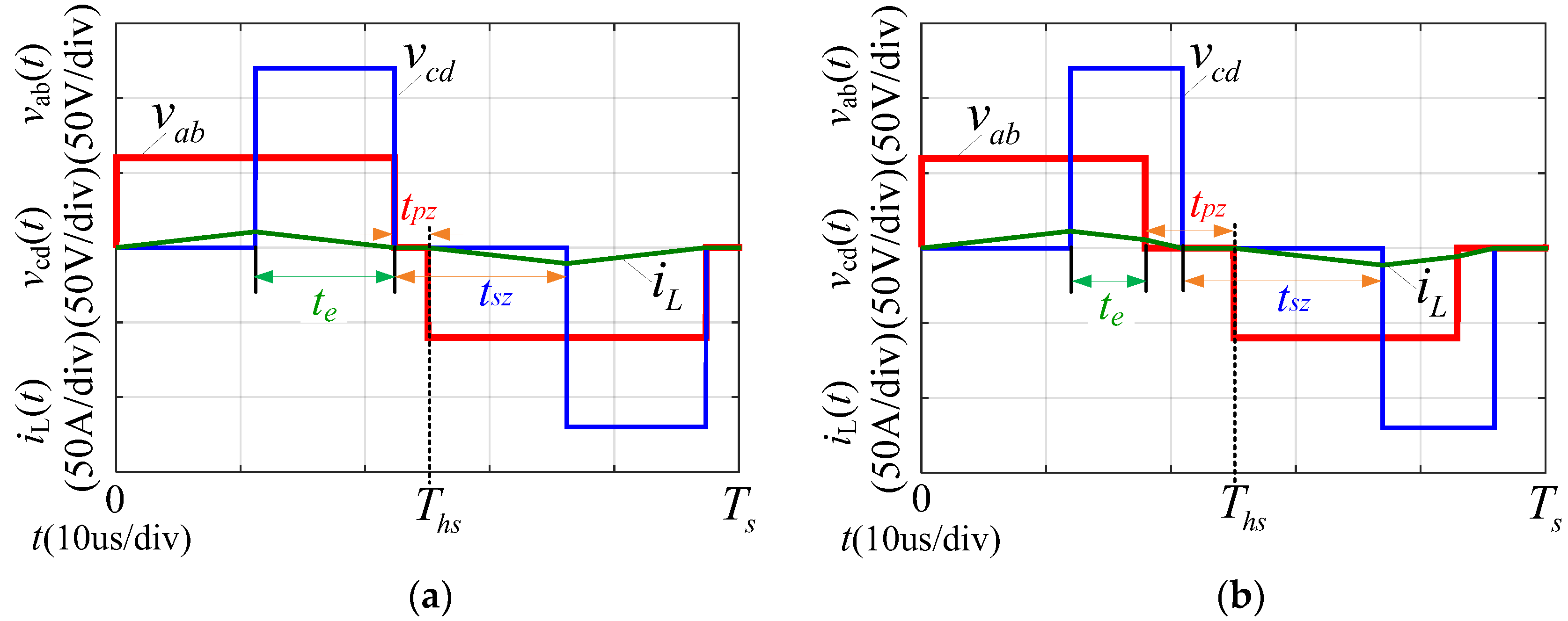
Figure 10a,b show the simulation waveforms of MNPC and GMBPC at low power level respectively when d = 2. Although the backflow power in these two control methods is zero, the non-active power transmission time is different. Under certain transmission power k = 0.2, δp, δs, and δe of MNPC are 89.4%, 44.7%, and 44.7%, respectively, while δp, δs, and δe of GMBPC are 71.7%, 35.9%, and 23.9%, respectively. Apparently, the effective power transmission time ratio δp, δs, and δe of MNPC are all larger than that of GMBPC. As a result, the optimized performance of MNPC is supposed to be better than optimized performance of GMBPC at low power level.
4.3. Minimum Non-Active Power Transmission Time Control at High Power Level
At high power level, the optimized control strategy will work in mode 5C. Based on the numerical optimization results in Appendix B, the minimum non-active power transmission time is always reached in mode 5Ca when d > 1 or in mode 5Cd when d < 1.
In mode 5Ca, the tpna, tsna and te can be calculated as:
As shown in Figure A1a, tsna is larger than tpna in mode 5Ca. Therefore, the ETR on the secondary side (i.e., δs) is smaller than the ETR on the primary side (i.e., δp). Moreover, as can be seen in Equation (38), the maximization of δe is equivalent to the minimization of γs. Therefore, the minimization of min (δp, δs) and the maximization of δe can be reached at the same time. The optimized control parameters are derived as below:
In mode 5Cd, the tpna, tsna and te can be calculated as:
Similar to the derivation process in mode 5Ca, the optimized control parameters in mode 5Cd can be derived as below:
Figure 11a,b show the simulation waveforms of MNPC and GMBPC at high power level, respectively, when d = 2. Under certain transmission power k = 0.4, δp, δs, and δe of MNPC are 87.8%, 42.4%, and 42.4%, respectively, while δp, δs, and δe of GMBPC are 79.7%, 39.3%, and 35.4%, respectively. Both the zero power transmission time and the equivalent zero power transmission time caused by backflow power of MNPC are smaller than that of GMBPC. As a result, power is transmitted more efficiently in MNPC than in GMBPC at high power level.
Equations (4) and (41) constitute the control parameters of MNPC when d is smaller than 1 while Equations (7) and (39) constitute the control parameters of MNPC when d is larger than 1. Similar to the GMBPC, MNPC also has only two subsections (i.e., low and high power level). The control parameters are piecewise continuous function with k. More than that, according to the optimized control parameters in Equations (4), (7), (39) and (41), MNPC method is exactly the same as the UTPS control method to minimize the current stress in whole load range in [9]. In other words, the minimum current stress and the minimum non-active transmission time can be reached at the same time.
4.4. Comparative Analysis of Minimum Nonactive Power Transmission Time Control
The overall performance of MNPC, GMBPC and SPS is compared as follows.
4.4.1. Backflow Power
The backflow power of MNPC, GMBPC and SPS versus k is plotted in Figure 12. The backflow power in MNPC is slightly larger than that in GMBPC. Moreover, the backflow power of MNPC and GMBPC is much smaller than the backflow power of SPS control especially at lower power level. In general, GMBPC has a better performance than MNPC on the reduction of backflow power.
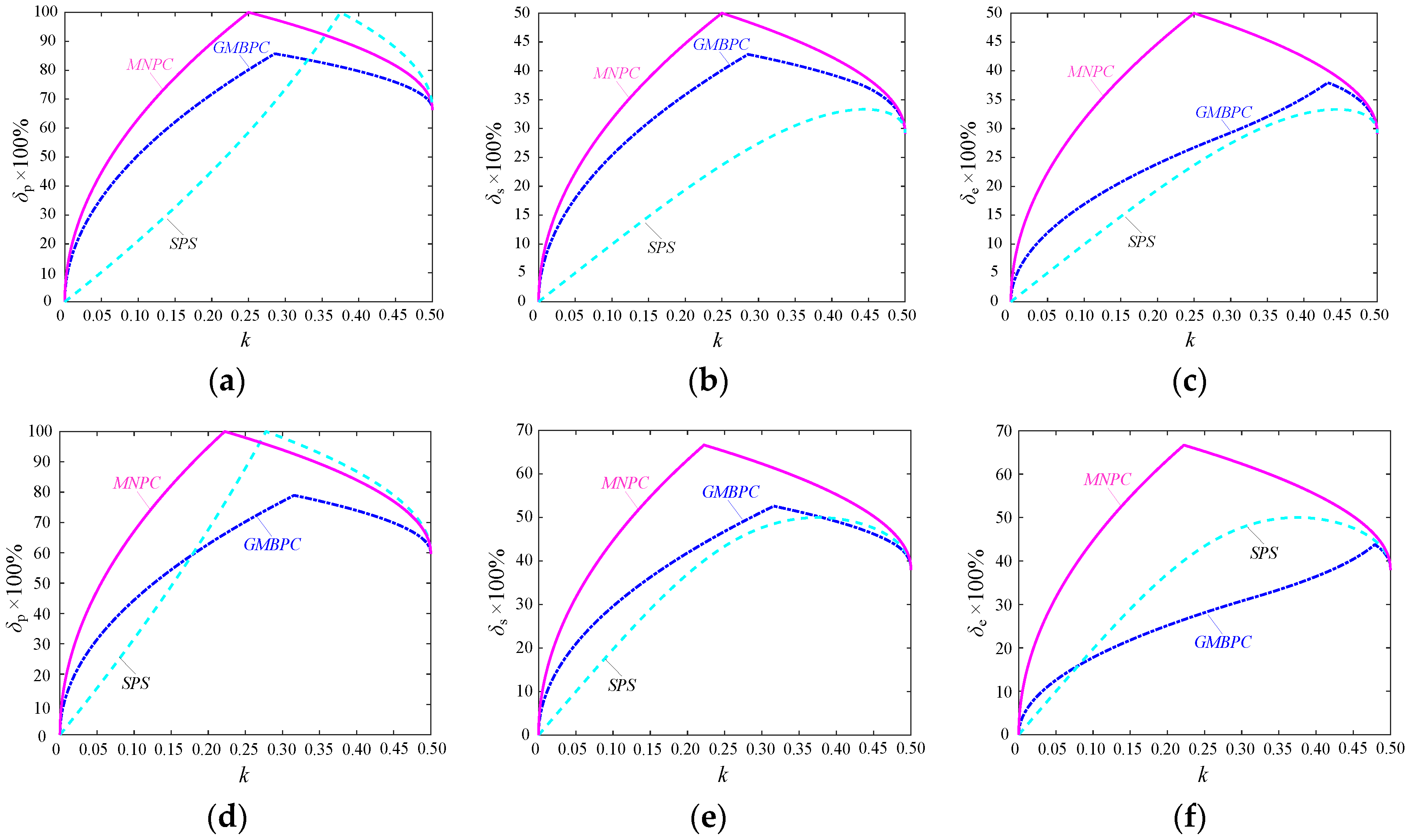
4.4.2. Effective Power Transmission Time Ratio
As shown in Figure 13, the maximum δp and δs in MNPC and GMBPC occur at the boundary between low power mode and high power mode. As shown in Figure 13a, δp in SPS is even larger than δp in MNPC and GMBPC at higher power level. However, δs in SPS is much smaller than δp in SPS. The operation performance is mostly determined by δe and the minimum value of δp and δs. Therefore, the performance of SPS is worse than that of MNPC and GMBPC.
When d = 2(V1 = 60 V, V2 = 120 V), the maximum values of δp, δs and δe of MNPC are 100%, 50% and 50%, respectively, while the maximum values of δp, δs and δe of GMBPC are 86%, 43% and 43%, respectively. Moreover, the δp, δs and δe in MNPC are always larger than that in GMBPC. Especially, the δe in MNPC is much larger than the δe in GMBPC and SPS. As a result, MNPC has a better performance than GMBPC on the reduction of non-active power transmission.When d reduces to 1.5(V1 = 80 V, V2 = 120 V), the δe in GMBPC, MNPC and SPS increases when d approaches to 1. However, the increase rate of δe in GMBPC is smaller than that of MNPC and SPS control. Therefore, δe in GMBPC is even smaller than δe in SPS control. It indicates that the performance of DAB may not be improved by GMBPC when d is close to 1.
4.4.3. Current Stress and Current rms
As shown in Figure 14a,b, the current stress and current rms of MNPC and GMBPC are reduced efficiently compared to that of SPS control when d = 2. Moreover, MNPC has the minimum current stress and minimum current RMS compared to other two methods. As a result, MNPC has a better performance of current than GMBPC. However, as can be seen in Figure 14c,d, when the voltage conversion ratio d is reduced to 1.5, the current stress and current rms of GMBPC are even larger than that of SPS control. The same conclusion can be drawn that the optimization of backflow power may not ensure the high-efficiency operation of DAB when d is close to 1.
4.4.4. Switching Characteristics
As analyzed in Section 3.5.4, all switching devices can achieve soft-switching in GMBPC. At high power level, all the switching devices can be turned on at ZVS for MNPC in mode 5C. At low power level, Q3 and Q4 are turned on at ZVS while Q1, Q2, Q5, Q6, Q7 and Q8 are turned off at ZCS for MNPC when d is smaller than 1. A similar situation can be seen when d is larger than 1. As a result, all the switching devices can achieve soft-switching at both low power level and high power level by MNPC and GMBPC.
4.4.5. Limitations of Backflow Power Optimization Methods
Unlike the SPS control, both MNPC and GMBPC can ensure soft-switching operation for all switching devices with arbitrary d. However, the effective power transmission time of GMBPC reduces a lot when d approaches to 1. This is because that the optimization of GMBPC does not take the zero power transmission into consideration. Minimum backflow power is obtained at the cost of increasing zero power transmission time when d is close to 1. It indicates that the current stress and rms value of GMBPC become larger than SPS control when d is close to 1. As a result, the advantage of full soft-switching in GMBPC may be counteracted by increasing current. In spite of this, GMBPC is still effective to improve the performance of DAB when d is far from 1.
5. Results
5.1. Implementation Method for GMBPC
The implementation method of MNPC is presented in [9]. Therefore, only the implementation of GMBPC is introduced in this section. Replacing the “d” in (17) and (33) by 1/d, the expressions of D1 and D2 can be interchangeable. Therefore, an implementation method is developed for GMBPC. As shown in Figure 7c, D1 and D2 changes monotonically with transmission power k. Therefore, the output of PI controller, i.e., m, can be used to denote D1 or D2 directly.
When d is larger than 1:
When d is smaller than 1:
The control structure for the GMBPC method is illustrated in Figure 15.
5.2. Experimental Results
An experimental prototype is built to verify the effectiveness of the proposed control method and theoretical analysis. Figure 16 is a photo of experimental prototype. The transformer turns ratio n is 1. Switching frequency fs is 20 kHz. The inductance L is 64 μH. All switching devices in both the primary H-bridge and secondary H-bridge are IXFX160N30TMOSFETs (IXYS, Lampertheim, Germany). The control system is based on the EP4CE15E22C8N FPGA (Altera, San Jose, CA, USA). The current waveforms are recorded by a Tektronix A622current probe (Tektronix, Beaverton, OR, USA). The current waveforms lag behind the voltage waveforms about 2 μs.
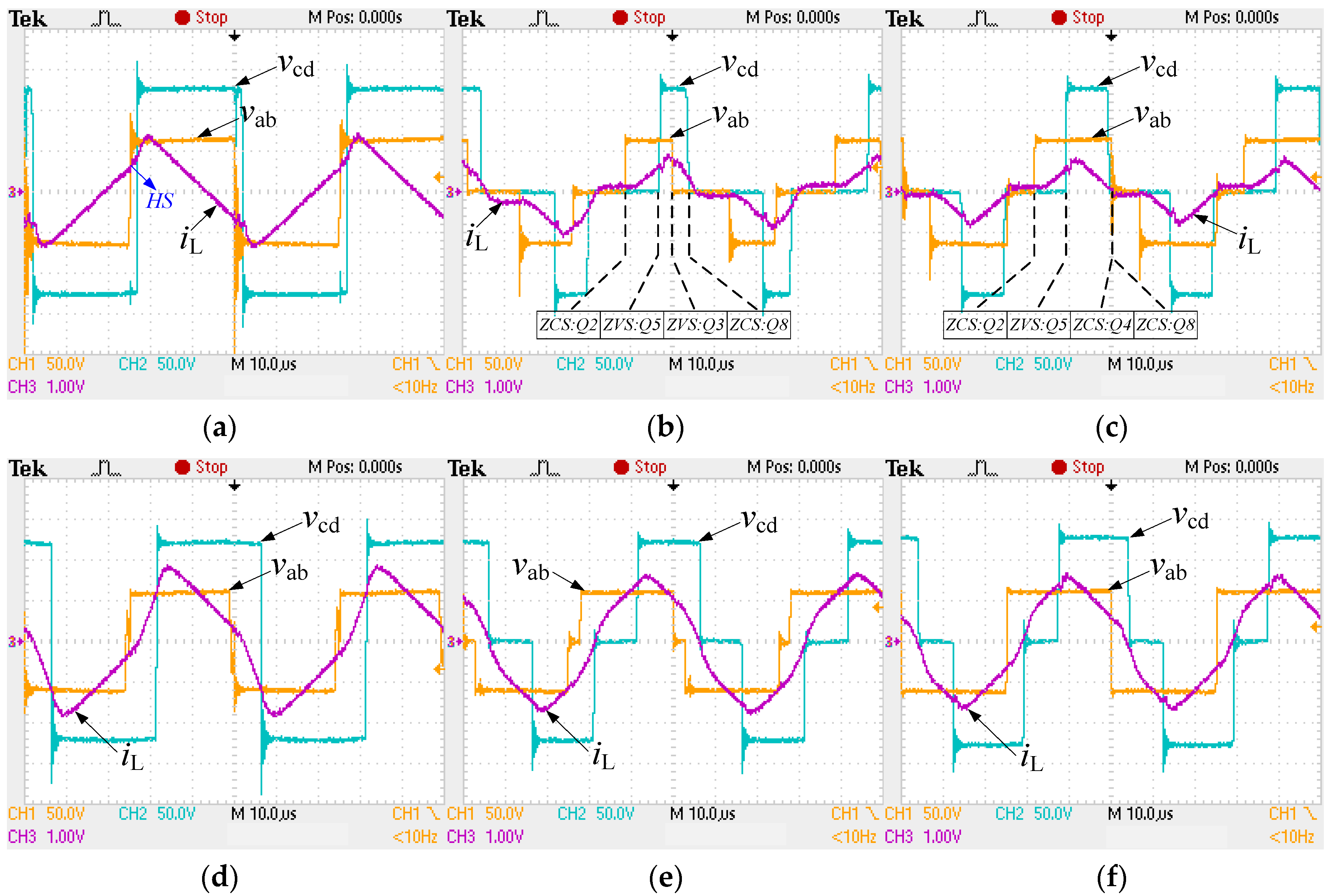
Figure 17 illustrates the operating waveforms when V1 = 120 V, V2 = 60 V while Figure 18 illustrates the operating waveforms when V1 = 60 V, V2 = 120 V. At low power level, i.e., Po = 144 W and k = 0.1, both MNPC and GMBPC have good effect on the reduction on the current stress and rms value.
In Figure 17a–c, the current stress is about 14 A with SPS, 9 A with GMBPC and 8 A with MNPC. MNPC has the minimum current stress. At high power level, i.e., Po = 500 W and k = 0.35, the difference of current stress and rms value between SPS and optimized methods is smaller than the difference at low power level. At low power level, Q5 to Q8 suffer the hard-switching operation with SPS control as shown in Figure 17a while Q1 to Q4 suffer the hard-switching operation with SPS control as shown in Figure 18a. As can be seen in Figure 17b,c and Figure 1b,c, all switching devices in GMBPC and MNPC can achieve soft-switching (ZVS or ZCS), leading to smaller voltage spikes for vab and vcd at switching moments. At high power level, the soft-switching cannot still be achieved in SPS control, as shown in Figure 17d and Figure 18d. However, the GMBPC and MNPC operate in mode 5C at high power level, so ZVS is guaranteed for all the switching devices. Experimental results verify the full soft-switching operation in whole load range by GMBPC and MNPC. Figure 19 shows the operating waveforms under V1 = 95 V, V2 = 120 V and Po = 230 W (k = 0.1). Because the voltage conversion ratio d is close to 1, the current stress in MNPC has little difference from the current stress in SPS control. However, as shown in Figure 19b, the current stress with GMPBC is larger than that with SPS control and MNPC. Based on the theoretical analysis, the current rms value with GMPBC is also larger than that with SPS control and MNPC in this case. Compared to SPS control, although the switching loss can be reduced with soft-switching in GMPBC, the conduction loss is increased with increasing current in this case. Therefore, the efficiency may not be improved by GMBPC when d is close to 1.
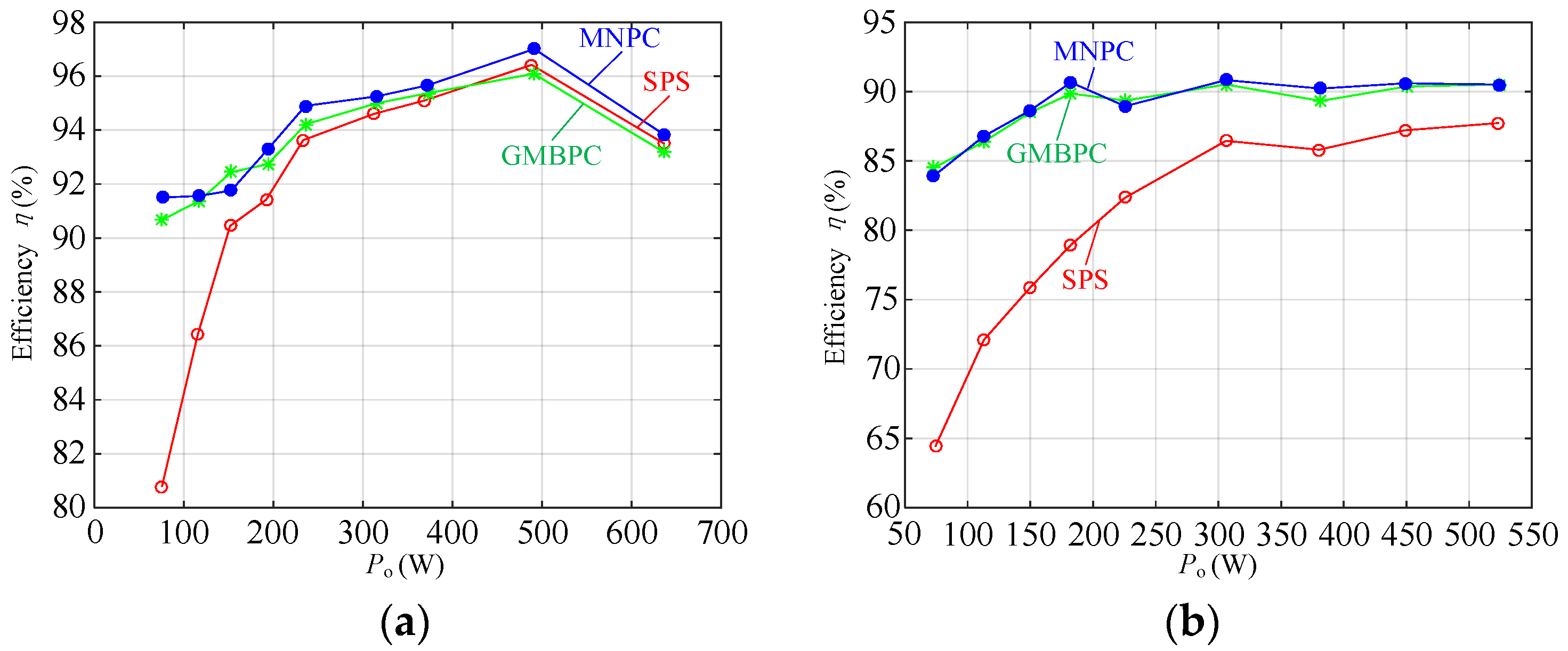
Figure 20a,b show the efficiency η varied with output power Po. The efficiency is improved a lot by GMBPC and MNPC especially at lower power level. At most of the operation points, MNPC has the highest efficiency than other two control methods.
In Figure 20a, the efficiency of GMBPC is lower than the efficiency of SPS control at higher power level. In Figure 20b, both GMBPC and MNPC has larger efficiency than SPS control. In general, GMBPC and MNPC are two effective methods to improve the performance of DAB especially when d is far from 1.
6. Conclusions
This paper proposes three optimized control methods for global minimum backflow power on the primary side, on the secondary side and on both sides, respectively. The comparative analysis results show that GMBPC has better performance than the other two optimized methods. GMBPC can reduce backflow power in both sides at the same time. The concept of maximum non-active power transmission time is proposed in this paper. The effective power transmission time ratio is maximized to improve the performance of DAB. The derived optimized control method, i.e., MNPC, achieves both the maximum effective power transmission time and minimum current stress of DAB at the same time. Comparative analysis shows that effective power transmission time ratio δe in GMBPC decreases when d approaches to 1 while δe in MNPC and SPS increases when d approaches to 1. The conclusion can be drawn that performance of DAB may not be improved by GMBPC when d is close to 1.Finally, a prototype is built to verify the effectiveness of theoretical analysis and the proposed control methods by experimental results.
Acknowledgments
The authors appreciate the support of China State Grid Company Research Project, “Basic theory and Simulation of AC&DC seamless hybrid flexible distribution networks” (PD71-17-024) and the support of “Fundamental Research Funds for the Central Universities” (E17JB00160).
Author Contributions
All authors made significant contributions to this research. More specifically, Fei Xiong performed the experiments, carried out the theoretical analysis and wrote the paper. Junyong Wu design the methodology and revised the paper. Liangliang Hao provided important comments on the paper’s structure. Zicheng Liu corrected the language and format of the paper.
Conflicts of Interest
The authors declare no conflicts of interest.
Parameter List
| V1 | dc-bus voltage on the primary side. |
| V2 | dc-bus voltage on the secondary side. |
| L | The inductance reflected to the primary side consist of leakage inductance and the additional complementary inductance. |
| n | Turns ratio. |
| φ | The outer phase shift ratio between the drive signals of Q1 (or Q2) and Q5 (or Q6). |
| D1 | The inner phase shift ratio in primary H-bridge between the drive signals of Q1 (or Q2) and Q3 (or Q4). |
| D2 | The inner phase shift ratio in secondary H-bridge between the drive signals of Q5 (or Q6) and Q7 (or Q8). |
| Ths | Half switching period. |
| A | The constant coefficient Ths/(2L). |
| k | Normalized transmission power to reference value AV1V2. |
| d | The voltage conversion ratio V2/V1. |
| vab | The output voltage in primary H-bridge. |
| vcd | The output voltage in secondary H-bridge. |
| iL | The transformer current. |
| Qp | The backflow power in primary side. |
| Qs | The backflow power in secondary side. |
| Qsum | The sum of backflow power in primary side and secondary side. |
| kimax | The maximum transmission power in mode i (i = 1, 2, 3, 4…). |
| tpz | The zero power transmission time in primary side. |
| tsz | The zero power transmission time in secondary side. |
| tpez | The maximum equivalent zero power transmission time in primary side. |
| tsez | The maximum equivalent zero power transmission time in secondary side. |
| tpna | The maximum nonactive power transmission time in primary side. |
| tsna | The maximum nonactive power transmission time in secondary side. |
| te | The effective power transmission time. |
| γp | The non-active power transmission time ratio (NTR) in primary side. |
| γs | The nonactive power transmission time ratio (NTR) in secondary side. |
| δp | The effective power transmission time ratio (ETR) in primary side. |
| δs | The effective power transmission time ratio (ETR) in secondary side. |
| δe | The effective power transmission time ratio. |
| m | The output of PI controller. |
Appendix A. Derivation Process for Objective 1 at Medium Power Level
Objective 1: Elimination of primary backflow power Qp with minimum secondary backflow power Qs:
The backflow power Qs in mode 5A is:
According to the expression of iL(t0), the following relationship can be obtained:
The optimized control parameters for minimum Qs are derived as:
It can be derived that current conditions for mode 5A, i.e., iL(t0) ≥ 0, iL(t1) ≥ 0, iL(t2) ≥ 0, and iL(t3) ≥ 0, are satisfied in (A4) so long as C ≤ 0. Taking derivative of Qs with respect to variable C, we can obtain:
Equation (A5) indicates that Qs reaches its minimum value exactly when C = 0, i.e., iL(t0) = 0. The optimized control parameters can be solved by substituting C = 0 into (A4), as shown in (20).
Appendix B. Derivation Process for MNPC at High Power Level
At high power level, the optimized control strategy will work in mode 5C. Six modes are distinguished in mode 5C with different non-active power transmission time, as shown in Figure A1. The constraint conditions in these modes are listed in Table A1.

Table A1.
Constraint conditions in Mode 5C.align equation in table.
| Mode | Constraints | te |
|---|---|---|
| Mode 5Ca | , | |
| Mode 5Cb | , , | |
| Mode 5Cc | , , | |
| Mode 5Cd | , | |
| Mode 5Ce | , , | |
| Mode 5Cf | , , |
Non-active power transmission time tpna, tsna and effective power transmission time te in these modes are listed in Table A2. Similar to [10,26], a numerical method is used to help to find the optimized operation mode.
Table A2.
Nonactive power transmission time in mode 5C.
| Mode | Nonactive Power Transmission Time tpna, tsna and Effective Power Transmission Time te |
|---|---|
| Mode 5Ca | |
| Mode 5Cb | |
| Mode 5Cc | |
| Mode 5Cd | |
| Mode 5Ce | |
| Mode 5Cf |
The values of te in mode 5C under different transmission power k are depicted in Figure A2. As shown in Figure A2, A, B and C are the optimized operation points under certain k with maximum te. The numerical optimization results indicate that the maximum te occurs only when D1 = 1 and d > 1 or when D2 = 1 and d < 1. The optimized control parameters can be derived just in these two operation modes. As a result, the derivation process can be simpler with the help of numerical optimization results.
Figure A1.
Six operating modes in mode 5C; (a) mode 5Ca; (b) mode 5Cb; (c) mode 5Cc; (d) mode 5Cd; (e) mode 5Ce; (f) mode 5Cf.
Figure A1.
Six operating modes in mode 5C; (a) mode 5Ca; (b) mode 5Cb; (c) mode 5Cc; (d) mode 5Cd; (e) mode 5Ce; (f) mode 5Cf.

Figure A2.
Effective power transmission time te versus transmission power k; (a) V1 = 60, V2 = 120 V; (b) V1 = 120, V2 = 60 V.
Figure A2.
Effective power transmission time te versus transmission power k; (a) V1 = 60, V2 = 120 V; (b) V1 = 120, V2 = 60 V.

References
- Martin-Arnedo, J.; Gonzalez-Molina, F.; Martinez-Velasco, J.; Adabi, M.E. EMTP Model of a Bidirectional Cascaded Multilevel Solid State Transformer for Distribution System Studies. Energies 2017, 10, 521. [Google Scholar] [CrossRef]
- Tan, N.M.L.; Abe, T.; Akagi, H. Design and Performance of a Bidirectional Isolated DC–DC Converter for a Battery Energy Storage System. IEEE Trans. Power Electron. 2012, 27, 1237–1248. [Google Scholar] [CrossRef]
- Wang, Z.; Liu, B.C.; Zhang, Y.; Cheng, M.; Chu, K.; Xu, L. The Chaotic-Based Control of Three-Port Isolated Bidirectional DC/DC Converters for Electric and Hybrid Vehicles. Energies 2016, 9, 83. [Google Scholar] [CrossRef]
- Zhao, B.; Song, Q.; Li, J.G.; Wang, Y.; Liu, W.H. Modular Multilevel High-Frequency-Link DC Transformer Based on Dual Active Phase-Shift Principle for Medium-Voltage DC Power Distribution Application. IEEE Trans. Power Electron. 2017, 32, 1779–1791. [Google Scholar] [CrossRef]
- Shi, Y.X.; Li, R.; Xue, Y.S.; Li, H. Optimized Operation of Current-Fed Dual Active Bridge DC–DC Converter for PV Applications. IEEE Trans. Ind. Electron. 2015, 62, 6986–6995. [Google Scholar] [CrossRef]
- Gammeter, C.; Krismer, F.; Kolar, J.W. Comprehensive Conceptualization, Design, and Experimental Verification of a Weight-Optimized All-SiC 2 kV/700 V DAB for an Airborne Wind Turbine. IEEE J. Emerg. Sel. Top. Power Electron. 2016, 4, 638–656. [Google Scholar] [CrossRef]
- Zhao, B.; Yu, Q.; Sun, W. Extended-Phase-Shift Control of Isolated Bidirectional DC-DC Converter for Power Distribution in Microgrid. IEEE Trans. Power Electron. 2012, 27, 4667–4680. [Google Scholar] [CrossRef]
- Zhao, B.; Song, Q.; Liu, W.H.; Sun, W.X. Current-Stress-Optimized Switching Strategy of Isolated Bidirectional DC-DC Converter with Dual-Phase-Shift Control. IEEE Trans. Ind. Electron. 2013, 60, 4458–4467. [Google Scholar] [CrossRef]
- Huang, J.; Wang, Y.; Li, Z.Q.; Li, W.J. Unified Triple-Phase-Shift Control to Minimize Current Stress and Achieve Full Soft-Switching of Isolated Bidirectional DC-DC Converter. IEEE Trans. Ind. Electron. 2016, 63, 4169–4179. [Google Scholar] [CrossRef]
- Krismer, F.; Kolar, J.W. Closed Form Solution for Minimum Conduction Loss Modulation of DAB Converters. IEEE Trans. Power Electron. 2012, 27, 174–188. [Google Scholar] [CrossRef]
- Tong, A.; Hang, L.; li, G.; jiang, X.; Gao, S. Modeling and Analysis of Dual-Active-Bridge Isolated Bidirectional DC/DC Converter to Minimize RMS Current. IEEE Trans. Power Electron. 2017. [Google Scholar] [CrossRef]
- Huang, J.; Wang, Y.; Gao, Y.; Lei, W.J.; Li, Y.F. Unified PWM Control to Minimize Conduction Losses Under ZVS in the Whole Operating Range of Dual Active Bridge Converters. In Proceedings of the 28th Annual IEEE Applied Power Electronics Conference and Exposition (APEC), Long Beach, CA, USA, 17–21 March 2013. [Google Scholar]
- Oggier, G.G.; Garcia, G.O.; Oliva, A.R. Modulation Strategy to Operate the Dual Active Bridge DC-DC Converter Under Soft Switching in the Whole Operating Range. IEEE Trans. Power Electron. 2011, 26, 1228–1236. [Google Scholar] [CrossRef]
- Wang, D.; Zhang, W.; Li, J. A PWM Plus Phase Shift Control Strategy for Dual-Active-Bridge DC-DC Converter in Electric Vehicle Charging/Discharging System. In Proceedings of the 2014 IEEE Conference and Expo on Transportation Electrification Asia-Pacific (ITEC Asia-Pacific), Beijing, China, 31 August–3 September 2014. [Google Scholar]
- Harrye, Y.A.; Ahmed, K.H.; Aboushady, A.A. Reactive Power Minimization of Dual Active Bridge DC/DC Converter with Triple Phase Shift Control using Neural Network. In Proceedings of the 2014 International Conference on Renewable Energy Research and Application (ICRERA), Milwaukee, WI, USA, 19–22 October 2014. [Google Scholar]
- Shi, X.; Jiang, J.; Guo, X. An Efficiency-Optimized Isolated Bidirectional DC-DC Converter with Extended Power Range for Energy Storage Systems in Microgrids. Energies 2013, 6, 27–44. [Google Scholar] [CrossRef]
- Rodriguez, J.R.; Venegas, R.V.; Moreno-Goytia, E.L. Single Loop, Zero Reactive Power in Dual-Active-Bridge Converters. In Proceedings of the 2013 IEEE International Autumn Meeting on Power, Electronics and Computing (ROPEC), Mexico City, Mexico, 13–15 November 2013. [Google Scholar]
- Bai, H.; Mi, C. Eliminate Reactive Power and Increase System Efficiency of Isolated Bidirectional Dual-Active-Bridge DC-DC Converters Using Novel Dual-Phase-Shift Control. IEEE Trans. Power Electron. 2008, 23, 2905–2914. [Google Scholar] [CrossRef]
- Karthikeyan, V.; Gupta, R. Zero circulating current modulation for isolated bidirectional dual-active-bridge DC-DC converter. IET Power Electron. 2016, 9, 1553–1561. [Google Scholar] [CrossRef]
- Hou, N.; Song, W. Full-bridge isolated DC/DC converters with triple-phase-shift control and soft starting control method. Proc. Chin. Soc. Electr. Eng. 2015, 35, 6113–6121. [Google Scholar]
- Xu, G.; Sha, D.; Zhang, J. Unified Boundary Trapezoidal Modulation Control Utilizing Fixed Duty Cycle Compensation and Magnetizing Current Design for Dual Active Bridge DC-DC Converter. IEEE Trans. Power Electron. 2017, 32, 2243–2252. [Google Scholar] [CrossRef]
- Sha, D.; Wang, X.; Chen, D. High Efficiency Current-Fed Dual Active Bridge DC–DC Converter with ZVS Achievement Throughout Full Range of Load Using Optimized Switching Patterns. IEEE Trans. Power Electron. 2017. [Google Scholar] [CrossRef]
- Wen, H.; Xiao, W.; Su, B. Nonactive Power Loss Minimization in a Bidirectional Isolated DC-DC Converter for Distributed Power Systems. IEEE Trans. Ind. Electron. 2014, 61, 6822–6831. [Google Scholar] [CrossRef]
- Chu, Y.; Wang, S. Bi-directional isolated DC-DC converters with reactive power loss reduction for electric vehicle and grid support applications. In Proceedings of the 2012 IEEE Transportation Electrification Conference and Expo (ITEC), Dearborn, MI, USA, 18–20 June 2012. [Google Scholar]
- Harrye, Y.A.; Ahmed, K.H.; Adam, G.P.; Aboushady, A.A. Comprehensive Steady State Analysis of Bidirectional Dual Active Bridge DC/DC Converter Using Triple Phase Shift Control. In Proceedings of the 2014 IEEE 23rd International Symposium on Industrial Electronics (ISIE), Istanbul, Turkey, 1–4 June 2014. [Google Scholar]
- Huang, J.; Wang, Y.; Li, Z.; Lei, W.J. Multifrequency approximation and average modelling of an isolated bidirectional dc-dc converter for dc Microgrids. IET Power Electron. 2016, 9, 1120–1131. [Google Scholar] [CrossRef]
Figure 1.
Topology of the DAB converter.

Figure 2.
Operating waveforms of selected modes with TPS control: (a) Definition of control parameters; (b) Mode 1; (c) Mode 2; (d) Mode 3; (e) Mode 4; (f) Mode 5.
Figure 2.
Operating waveforms of selected modes with TPS control: (a) Definition of control parameters; (b) Mode 1; (c) Mode 2; (d) Mode 3; (e) Mode 4; (f) Mode 5.

Figure 3.
Operating waveforms of SPS control.
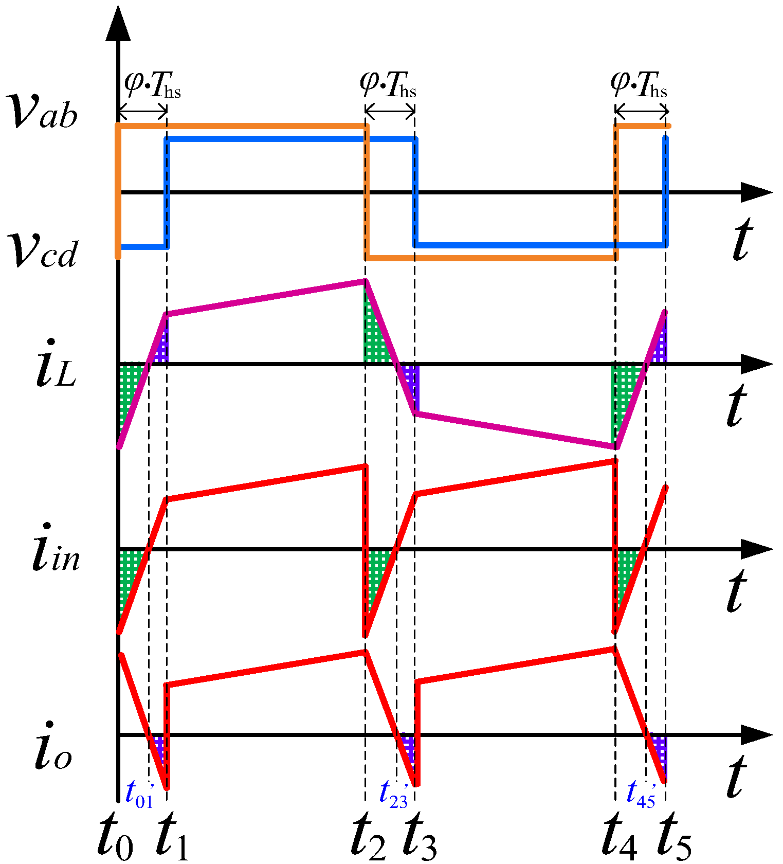
Figure 4.
Maximum transmission power kmax in mode 1 to mode 4 versus voltage conversion ratio d.

Figure 5.
Operating waveforms of selected modes in mode 5: (a) Mode 5A; (b) Mode 5B; (c) Mode 5C.
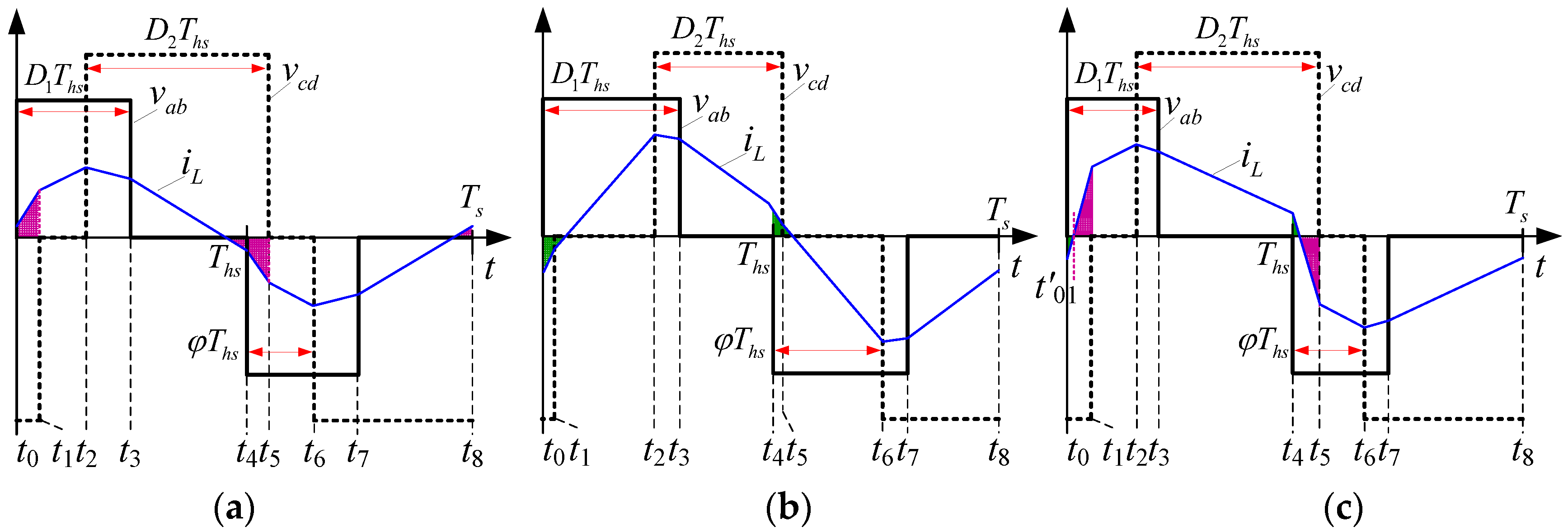
Figure 6.
The backflow power of GMPBPC, GMSBPC, GMBPC and traditional SPS control method; (a–c) are plotted for V1 = 60 V, V2 = 120 V; (d–f) are plotted for V1 = 120 V, V2 = 60 V.
Figure 6.
The backflow power of GMPBPC, GMSBPC, GMBPC and traditional SPS control method; (a–c) are plotted for V1 = 60 V, V2 = 120 V; (d–f) are plotted for V1 = 120 V, V2 = 60 V.

Figure 7.
Control Parameters of optimized control methods under V1 = 60 V, V2 = 120 V; (a) GMPBPC; (b) GMSBPC; (c) GMBPC.
Figure 7.
Control Parameters of optimized control methods under V1 = 60 V, V2 = 120 V; (a) GMPBPC; (b) GMSBPC; (c) GMBPC.

Figure 8.
Current stress and current RMS of optimized control methods; (a) Current stress under V1 = 60 V, V2 = 120 V; (b) Current stress under V1 = 120 V, V2 = 60 V; (c) Current RMS under V1 = 60 V, V2 = 120 V; (d) Current RMS under V1 = 120 V, V2 = 60 V.
Figure 8.
Current stress and current RMS of optimized control methods; (a) Current stress under V1 = 60 V, V2 = 120 V; (b) Current stress under V1 = 120 V, V2 = 60 V; (c) Current RMS under V1 = 60 V, V2 = 120 V; (d) Current RMS under V1 = 120 V, V2 = 60 V.

Figure 9.
Non-active power transmission time in (a) Primary side; (b) Secondary side.

Figure 10.
Simulation waveforms of MNPC and GMBPC at low power level under V1 = 60 V, V2 = 120 V; (a) MNPC; (b) GMBPC.
Figure 10.
Simulation waveforms of MNPC and GMBPC at low power level under V1 = 60 V, V2 = 120 V; (a) MNPC; (b) GMBPC.

Figure 11.
Simulation waveforms of MNPC and GMBPC at high power level under V1 = 60 V, V2 = 120 V; (a) MNPC; (b) GMBPC.
Figure 11.
Simulation waveforms of MNPC and GMBPC at high power level under V1 = 60 V, V2 = 120 V; (a) MNPC; (b) GMBPC.

Figure 12.
Backflow power of MNPC, GMBPC and SPS versus k under V1 = 60 V, V2 = 120 V; (a) Qp; (b) Qs; (c) Qsum.
Figure 12.
Backflow power of MNPC, GMBPC and SPS versus k under V1 = 60 V, V2 = 120 V; (a) Qp; (b) Qs; (c) Qsum.
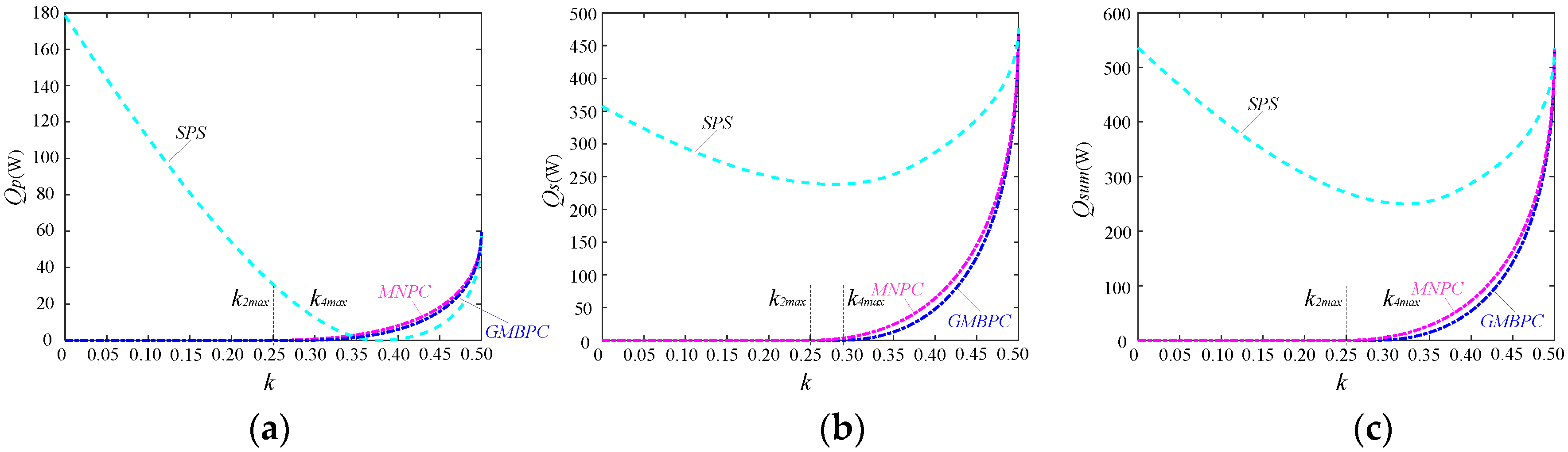
Figure 13.
Effective power transmission time ratio of MNPC, GMBPC and SPS versus k under V1 = 60 V, V2 = 120 V; (a) δp; (b) δs; (c) δe and V1 = 80 V, V2 = 120 V; (d) δp; (e) δs; (f) δe.
Figure 13.
Effective power transmission time ratio of MNPC, GMBPC and SPS versus k under V1 = 60 V, V2 = 120 V; (a) δp; (b) δs; (c) δe and V1 = 80 V, V2 = 120 V; (d) δp; (e) δs; (f) δe.

Figure 14.
Current stress and current rms of MNPC, GMBPC and SPS control method. (a) Current stress under V1 = 60 V, V2 = 120 V; (b) Current rms under V1 = 60 V, V2 = 120 V; (c) Current stress under V1 = 80 V, V2 = 120 V; (d) Current rms under V1 = 80 V, V2 = 120 V.
Figure 14.
Current stress and current rms of MNPC, GMBPC and SPS control method. (a) Current stress under V1 = 60 V, V2 = 120 V; (b) Current rms under V1 = 60 V, V2 = 120 V; (c) Current stress under V1 = 80 V, V2 = 120 V; (d) Current rms under V1 = 80 V, V2 = 120 V.
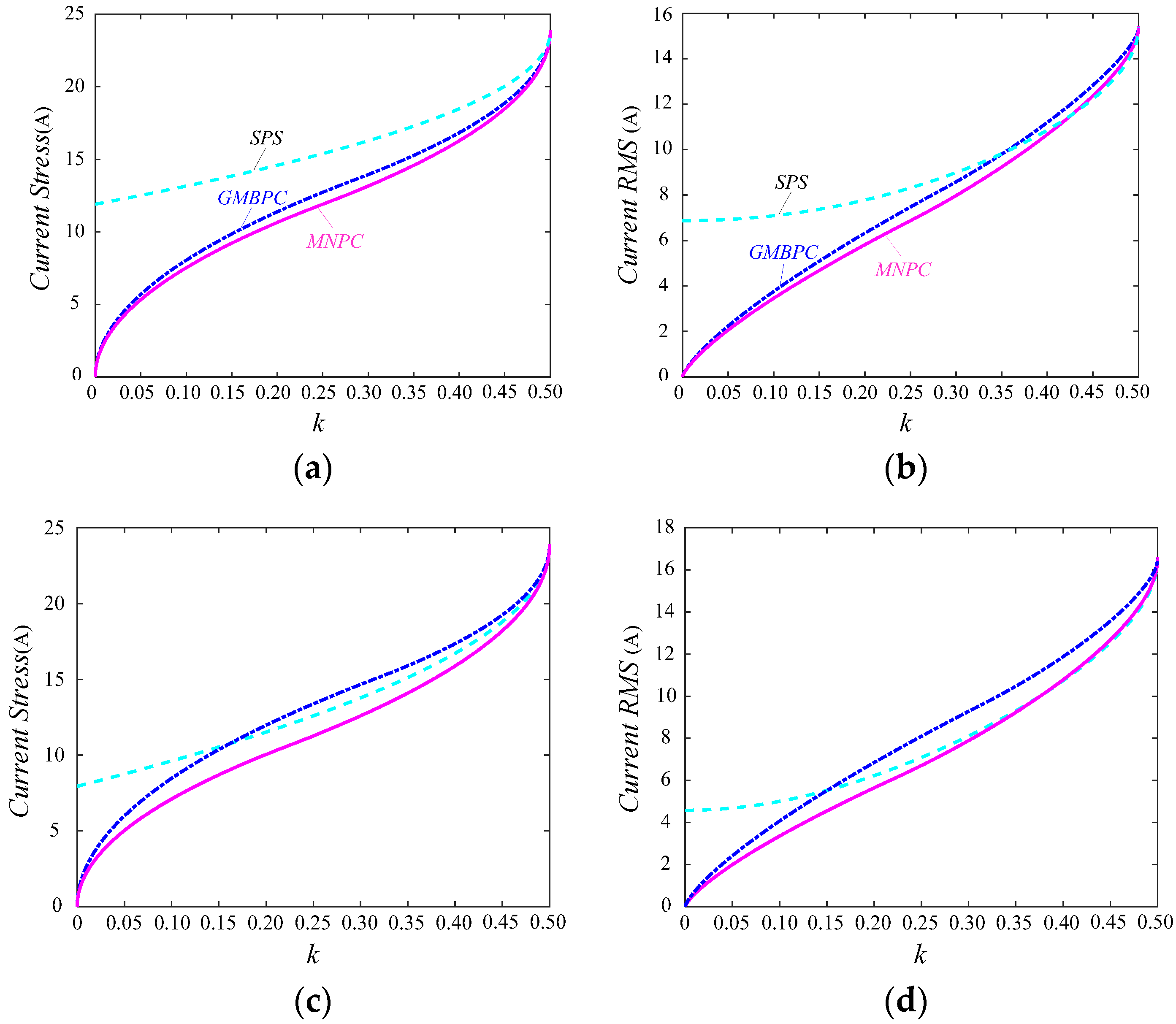
Figure 15.
Control structure for the GMBPC method.
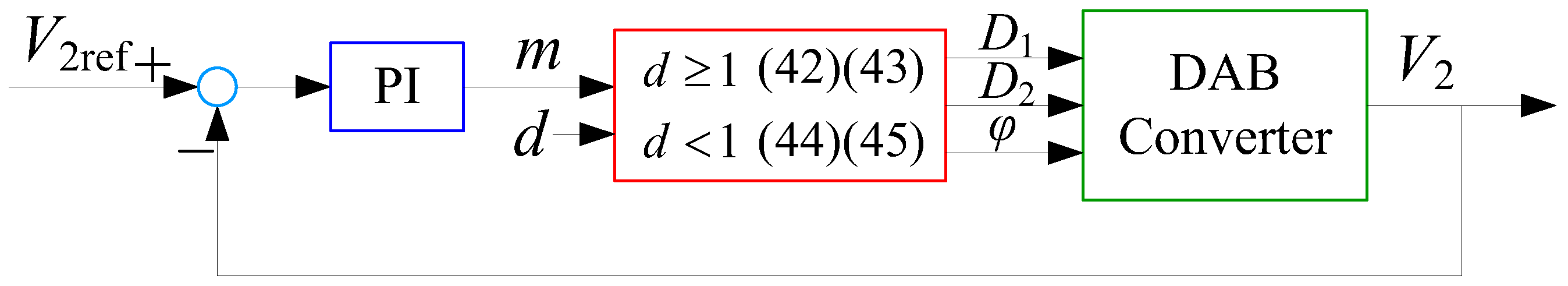
Figure 16.
Experimental prototype.
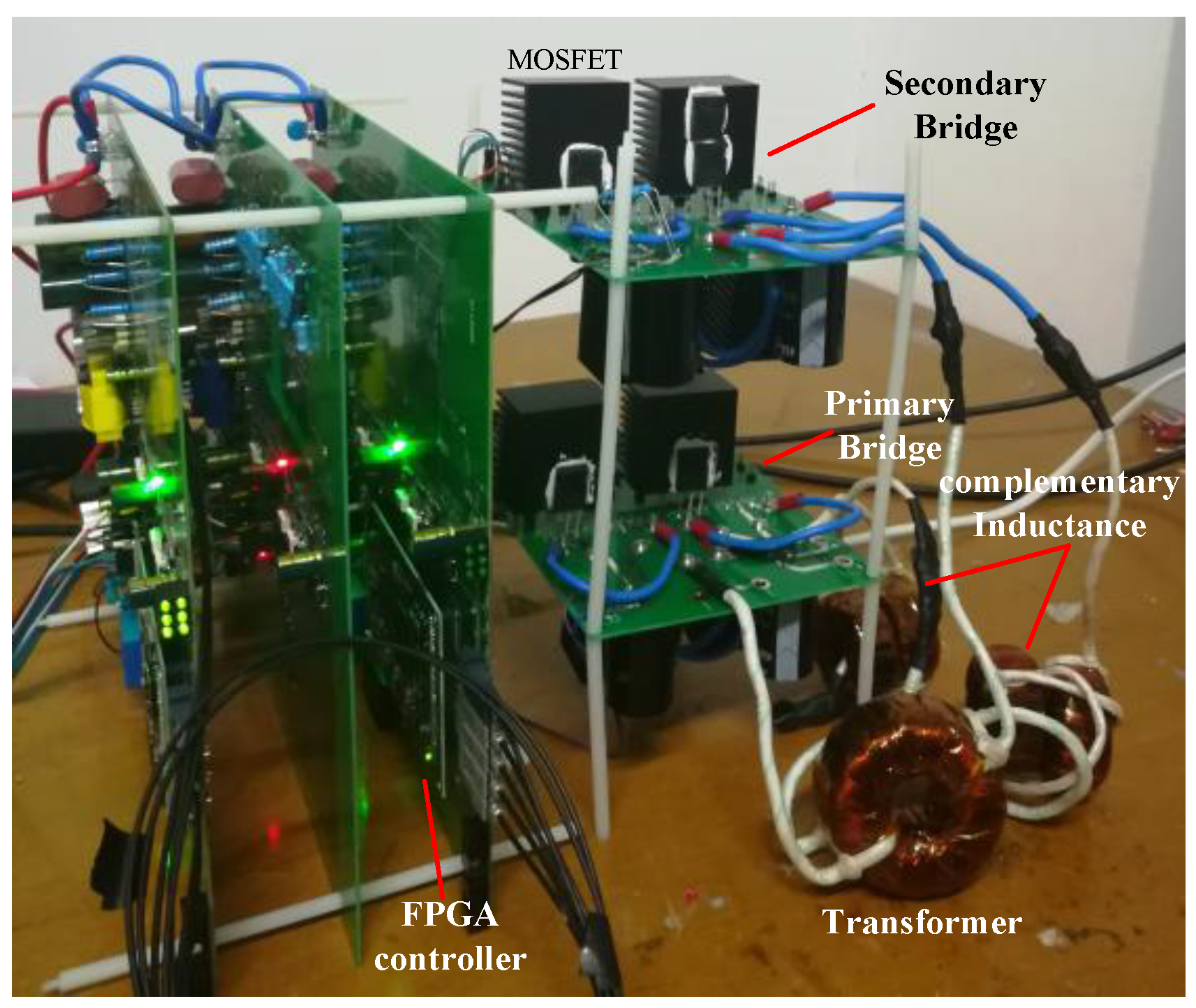
Figure 17.
Operating waveforms under V1 = 120 V, V2 = 60 V, Po = 144 W; (a) SPS; (b) GMBPC; (c) MNPC and Po = 500 W; (d) SPS; (e) GMBPC; (f) MNPC (vab = 50 V/div, vcd = 50 V/div, iL = 10 A/div).
Figure 17.
Operating waveforms under V1 = 120 V, V2 = 60 V, Po = 144 W; (a) SPS; (b) GMBPC; (c) MNPC and Po = 500 W; (d) SPS; (e) GMBPC; (f) MNPC (vab = 50 V/div, vcd = 50 V/div, iL = 10 A/div).
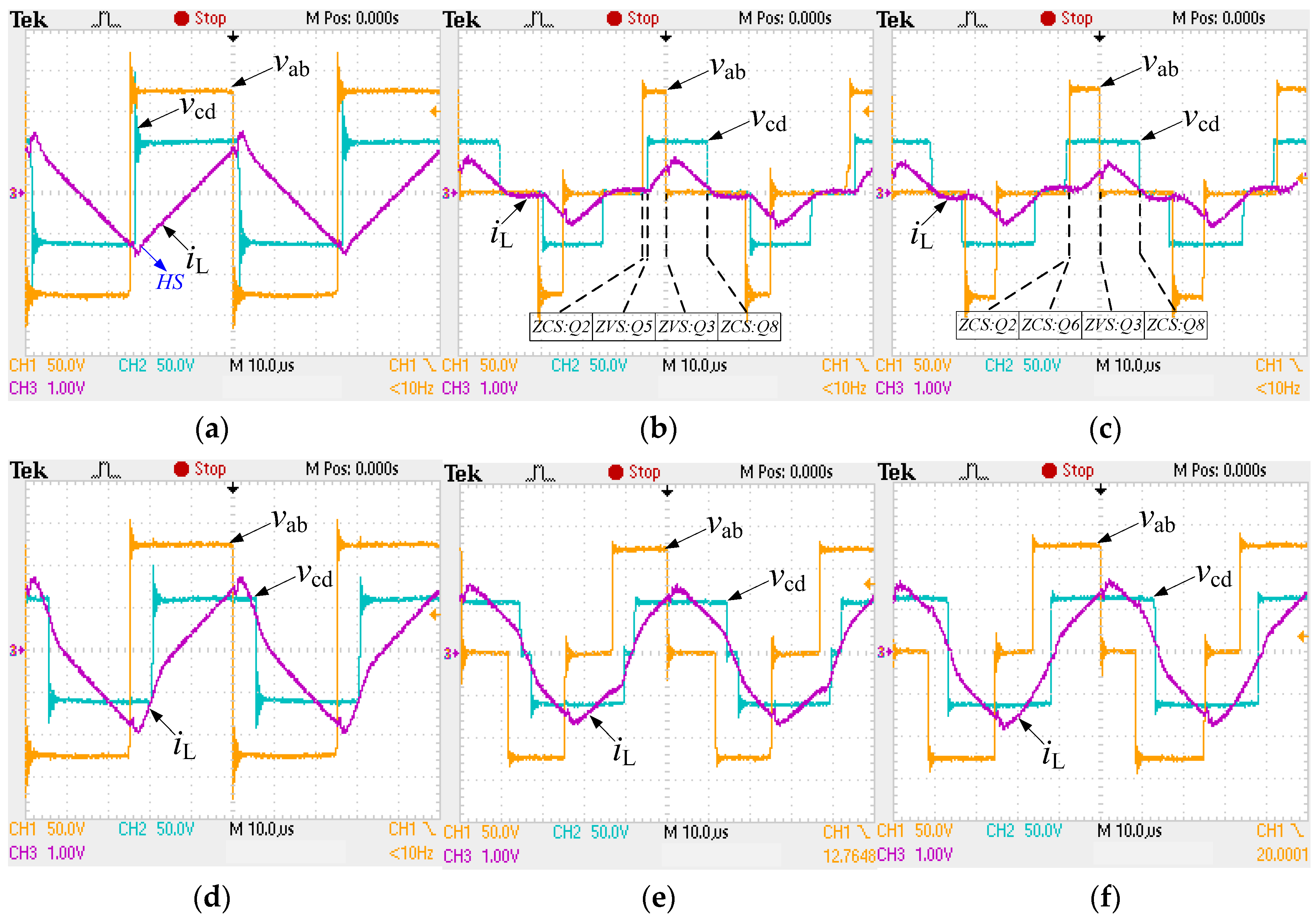
Figure 18.
Operating waveforms under V1 = 60 V, V2 = 120 V, Po = 144 W; (a) SPS; (b) GMBPC; (c) MNPC and Po = 500 W; (d) SPS; (e) GMBPC; (f) MNPC (vab = 50 V/div, vcd = 50 V/div, iL = 10 A/div).
Figure 18.
Operating waveforms under V1 = 60 V, V2 = 120 V, Po = 144 W; (a) SPS; (b) GMBPC; (c) MNPC and Po = 500 W; (d) SPS; (e) GMBPC; (f) MNPC (vab = 50 V/div, vcd = 50 V/div, iL = 10 A/div).

Figure 19.
Operating waveforms under V1 = 95 V, V2 = 120 V, Po = 230 W; (a) SPS; (b) GMBPC; (c) MNPC.
Figure 19.
Operating waveforms under V1 = 95 V, V2 = 120 V, Po = 230 W; (a) SPS; (b) GMBPC; (c) MNPC.
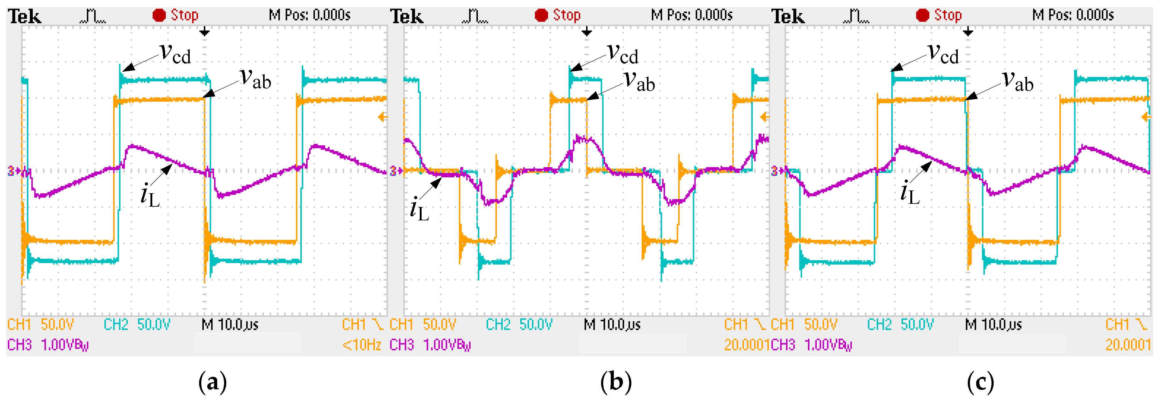
Figure 20.
Efficiency varied with output power Po; (a) V1 = 120 V, V2 = 60 V; (b) V1 = 60 V, V2 = 120 V.
Figure 20.
Efficiency varied with output power Po; (a) V1 = 120 V, V2 = 60 V; (b) V1 = 60 V, V2 = 120 V.

Table 1.
Operation constraints and transmission power for selected modes.
| Modes | Mode Constraints (D1 and D2 ≤ 1) | Transmission Power k |
|---|---|---|
| Mode 1 | D1 − D2 ≤ φ ≤ 0 | k = D1(D2 − D1 + 2φ) |
| Mode 2 | 0 ≤ φ ≤ D1 − D2 | k = D2(D2 − D1 + 2φ) |
| Mode 3 | D1 ≤ φ ≤ 1 − D2 | k = D1D2 |
| Mode 4 | max(D1 − D2,0) ≤ φ ≤ min(1 − D2,D1) | k = −D12 − φ2 + 2D1φ + D1D2 |
| Mode 5 | 1 − D2 ≤ φ ≤ D1 | k = −D12 − D22 − 2φ2 + 2φ + 2D1φ − 2D2φ + D1D2 + 2D2 − 1 |
Table 2.
Control parameters and the power range of backflow power optimal control methods.
| Modes | GMPBPC | GMSBPC | GMBPC |
|---|---|---|---|
| Low Power Level | |||
| Power Range | |||
| Medium Power Level | |||
| Power Range | |||
| High PowerLevel | |||
| Power Range | |||
© 2017 by the authors. Licensee MDPI, Basel, Switzerland. This article is an open access article distributed under the terms and conditions of the Creative Commons Attribution (CC BY) license (http://creativecommons.org/licenses/by/4.0/).
Share and Cite
MDPI and ACS Style
Xiong, F.; Wu, J.; Hao, L.; Liu, Z. Backflow Power Optimization Control for Dual Active Bridge DC-DC Converters. Energies 2017, 10, 1403. https://doi.org/10.3390/en10091403
AMA Style
Xiong F, Wu J, Hao L, Liu Z. Backflow Power Optimization Control for Dual Active Bridge DC-DC Converters. Energies. 2017; 10(9):1403. https://doi.org/10.3390/en10091403
Chicago/Turabian StyleXiong, Fei, Junyong Wu, Liangliang Hao, and Zicheng Liu. 2017. "Backflow Power Optimization Control for Dual Active Bridge DC-DC Converters" Energies 10, no. 9: 1403. https://doi.org/10.3390/en10091403
Note that from the first issue of 2016, this journal uses article numbers instead of page numbers. See further details here.