Selection of Optimal Polymerization Degree and Force Field in the Molecular Dynamics Simulation of Insulating Paper Cellulose


1
College of Engineering and Technology, Southwest University, Chongqing 400715, China
2
State Grid Chongqing Electric Power Co. Chongqing Electric Power Research Institute, Chongqing 401123, China
3
Laboratory of Power Transmission Equipment & System Security and New Technology, Chongqing University, Chongqing 400044, China
*
Author to whom correspondence should be addressed.
Energies 2017, 10(9), 1377; https://doi.org/10.3390/en10091377
Submission received: 22 August 2017
/
Revised: 5 September 2017
/
Accepted: 8 September 2017
/
Published: 11 September 2017
Abstract
:To study the microscopic thermal aging mechanism of insulating paper cellulose through molecular dynamics simulation, it is important to select suitable DP (Degree of Polymerization) and force field for the cellulose model to shorten the simulation time and obtain correct and objective simulation results. Here, the variation of the mechanical properties and solubility parameters of models with different polymerization degrees and force fields were analyzed. Numerous cellulose models with different polymerization degrees were constructed to determine the relative optimal force field from the perspectives of the similarity of the density of cellulose models in equilibrium to the actual cellulose density, and the volatility and repeatability of the mechanical properties of the models through the selection of a stable polymerization degree using the two force fields. The results showed that when the polymerization degree was more than or equal to 10, the mechanical properties and solubility of cellulose models with the COMPASS (Condensed-phase Optimized Molecular Potential for Atomistic Simulation Studies) and PCFF (Polymer Consistent Force Field) force fields were in steady states. The steady-state density of the cellulose model using the COMPASS force field was closer to the actual density of cellulose. Thus, the COMPASS force field is favorable for molecular dynamics simulation of amorphous cellulose.
1. Introduction
Oil-paper insulation is the main form of insulation for large power transformers. Cellulose is an important component of insulating paper; therefore, the properties of cellulose not only decide the properties of insulating paper, but also the service life of transformers. Aging of the oil-paper insulation of a transformer is a very complex physical and chemical process. Thus, it is difficult to give an in-depth explanation for the aging process from the microscopic mechanism in the traditional study of insulation aging. However, the molecular structure of materials can be investigated through molecular dynamics simulation, which is helpful to analyze the microscopic mechanisms governing various complex macroscopic phenomena, allowing the connection between microscopic structures and macroscopic properties to be revealed [1,2].
During molecular dynamics simulation, especially of insulating paper cellulose, the selection of the polymerization degree and force field of the calculation model is very important to obtain correct simulation results and shorten the simulation time. Polymerization degree is an index to measure the size of a polymer molecule based on the number of repeating units; that is, the average value [3,4,5] of the number of repeating units in the polymer macromolecular chain. Molecular dynamics simulation uses computer technology, and the computer simulation time lengthens greatly with the increase of the polymerization degree of the cellulose model. There is a certain randomness in the selection of the existing polymerization degree [6,7,8,9,10]; for example, the cellulose polymerization degree used by K. Mazeau and L. Heux [11] was 10, that adopted by A. Paajanen and J. Vaari [12] was 16, other scholars have used 20 and 30, and that adopted by Zhu Mengzhao [13] was 40, etc. Therefore, further studies are required to confirm how to select a relative appropriate polymerization degree of the cellulose model used in molecular dynamics simulation to reflect the actual basic characteristics of cellulose and minimize the time of analog simulation.
The force field is called the soul of molecular mechanics and molecular dynamics. The choice of force field directly determines the accuracy of simulation results. Thus, force field selection is an important part of any simulation, and the study of force fields is of great importance [14]. At present, the force fields used in the molecular dynamics simulation of insulating paper cellulose mainly include PCFF (Polymer Consistent Force Field) and COMPASS (Condensed-phase Optimized Molecular Potential for Atomistic Simulation Studies) force fields. The selection of different force fields may cause great differences between the simulation and experimental results and induce uncertainties in the subsequent studies of microscopic mechanisms. However, there is no consensus on the best force field to select [15,16,17,18,19,20]. For example, W. Chen [21] used the PCFF force field, while Bazooyar, F. and Momany, F.A. [22] adopted the COMPASS force field. Therefore, similar to the case for the selection of the polymerization degree, further studies are required to confirm which force field should be selected to reflect the actual basic characteristics of cellulose to obtain more accurate simulation results.
Because there have been few studies on the selection of the optimal polymerization degree and force field in the molecular dynamics simulation of insulating paper cellulose, a large number of models are considered in this paper. The polymerization degree selection range of the model used for cellulose simulation was obtained through nearly six months of analog simulation and data analysis. The relative optimal force field was determined from the perspectives of the degree of closeness between the steady-state density of the cellulose model and the actual cellulose density, volatility, and repeatability of the mechanical properties of the model.
2. Selection of the Polymerization Degree of Cellulose Models
2.1. Models Building
To determine the variation of the mechanical properties and solubility of the cellulose chain, models of 19 groups of single cellulose chains in the amorphous region with the polymerization degrees of 2, 4, 6, 8, 9, 10, 12, 16, 20, 25, 30, 35, 40, 50, 60, 70, 80, 90, and 100 were constructed using COMPASS and PCFF force fields. The model density obtained by W. Chen [21] was about 1.385 g/cm3, while K. Mazeau and L. Heux [11] achieved a model with four different densities of 1.34–1.3927 g/cm3 by modeling with the same method and standpoint, and proposed that the density of cellulose in the amorphous region is 1.28–1.44 g/cm3. Therefore, we set the initial density of the model as 0.6 g/cm3, and the density of the 19 models was increased to approximately 1.40 g/cm3 through pressurization. The model construction is shown in Figure 1.
2.2. Parameters Setting
The cellulose models were constructed using Materials Studio software (Accelrys, San Diego, CA, USA). During the optimization of the molecular dynamics simulations and energies, the pressure intensity was set as 0.2 GPa, the Berendsen method [23] was used as the control method, the Andersen method [24] was used for temperature control, the Boltzmann distribution method was employed to randomize the starting speed, the atom-based method was used to describe van der Waals force interactions, the velocity verlet algorithm was adopted as the integration algorithm, and the Ewald method was used to model electrostatic interactions. The non-bond cutoff was 0.95 nm, the buffer width was 0.05 nm, and the spline width was 0.1 nm. The maximum number of iterations was 500, the time was 500 ps, the periodic boundary condition was adopted in the whole simulation process, and the simulation temperature was 298 K.
2.3. Analysis of Mechanical Properties
In elastic mechanics, tensile modulus (E) is the ratio of stress to strain and represents the material rigidity; a large E means high rigidity and strong resistance to deformation, as one of the mechanical property indices of materials. The shear modulus (G), also called the rigidity modulus, is the ratio of shear stress to strain. G indicates the shear resistance of the material. The poisson’s ratio (v) is the ratio of lateral strain to longitudinal deformation, and it is an elastic constant that reflects the transverse deformation of a material. The Cauchy pressure (C12-C44) can be used to measure the ductility of materials. The bulk modulus (K) describes the elasticity of homogeneous isotropic solids [25,26,27,28].
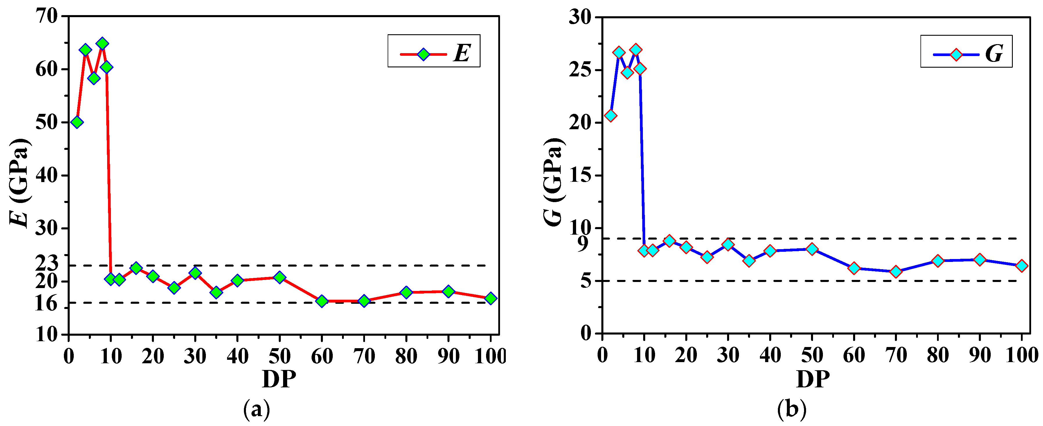
The changes of E and G of the models of 19 groups of single cellulose chains in the amorphous region with increasing DP from 2 to 100 under the two force fields were determined through analog computation and are shown in Figure 2 and Figure 3.
From Figure 2, we can conclude that E is maintained at 50–70 GPa and G at 20–28 GPa with increasing DP (DP = 2–10) under the COMPASS force field; when DP = 10, E and G suddenly decrease drastically; when DP = 10–100, E is basically maintained at 13.5–20 GPa and G at 5–8 GPa. Figure 3 reveals that the variations of E and G with a DP determined using the PCFF force field are basically consistent with those obtained with the COMPASS force field; that is, when DP is 10, a sudden change occurs, and then the values become stable.
The average values of E, G, v, and C12-C44 obtained by the calculation on the 14 sets of data (DP = 10, 12, 16, 20, 25, 30, 35, 40, 50, 60, 70, 80, 90, and 100) when the mechanic parameters (E, G, v, and C12-C44) reached the steady state are listed in Table 1. The average value of E obtained using the COMPASS force field is similar to the previously obtained E (14.24 GPa) and G (5.435 GPa) [10] and E of a cellulose amorphous region (12.79 GPa) [29], so the values conform to the actual mechanical properties of natural cellulose. The average values of E, G, v, and C12-C44 obtained using the PCFF force field differ slightly from those in References [10,29]. The sudden change of the mechanical properties when DP = 10 is possibly caused by the excessively short cellulose chain behaving in a manner that is inconsistent with the basic characteristics of cellulose polysaccharide (C6H10O5)n and the basic structure of cellulose, which is shown in Figure 4. When DP = 10, the mechanical properties of the cellulose model reach a steady state, and conform to the actual mechanical properties of the natural cellulose. Therefore, the polymerization degree of the model used in a molecular dynamics simulation of cellulose should not be less than 10.
2.4. Solubility Analysis
In relevant studies on solubility, the condensed state is selected for materials with both high and low molecular weight. The aggregation state of a material is determined by the geometrical arrangement of molecules, as are the physical properties of the material. The intermolecular force in the aggregation state is the non-bonding interatomic action force, rather than the chemical bond force, and can be divided into the van der Waals force (dispersion force, induction force, and dipole force) and hydrogen bonding force. In general, the cohesive energy density or solubility parameter is used to represent the intermolecular force in a material. The cohesive energy density (CED) can be expressed as:
where Ece represents the cohesive energy of the system, V is the volume of the whole system, Einter represents the total energy of all molecules, Etotal represents the total energy of the whole system, Eintra represents the intermolecular energy, and { } represents the average system in the NVT (fixed values of particle number N, volume P, and temperature T)/NPT (fixed values of particle number N, pressure P, and temperature T) ensemble.
The solubility parameter (δ) is used to evaluate the strength of the intermolecular force and determine the degree of compatibility between materials; δ can be expressed as:
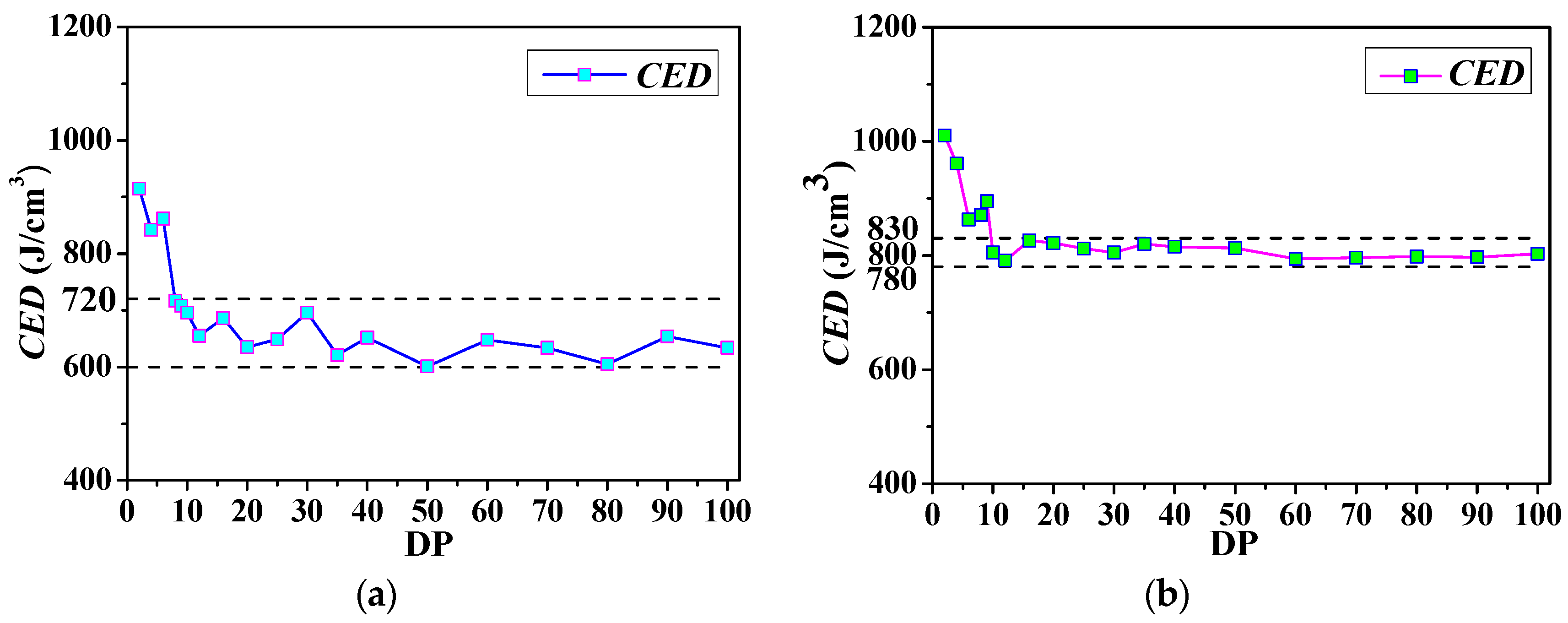
The variation of CED with polymerization degree determined using the COMPASS and PCFF force fields are presented in Figure 5, and δ obtained using the two force fields in a steady state are listed in Table 2.
Figure 5 reveals that, using the COMPASS force field, CED is 850–900 J/cm3 when DP is less than 6. When DP is equal to 6, CED suddenly decreases, and when DP is greater than 6, CED is stable in the range of 600–720 J/cm3. The average δ for the 10 groups with DP of 10–100 is 25.4 (J/cm3)0.5, this value is basically identical to those values obtained previously from (20.686 (J/cm3)0.5) [30], (18.03 (J/cm3)0.5) [31] and (20.6 (J/cm3)0.5) [32], which means that it is consistent with the actual chemical properties of cellulose.
Using the PCFF force field, CED is 850–1000 J/cm3 when DP is less than 6 (Figure 5b). When DP is equal to 10, CED suddenly decreases, and when DP is greater than 10, CED is stable in the range of 780–830 J/cm3. The average δ of the 10 groups with DP of 10–100 is 28.4 (J/cm3)0.5. This value is slightly different from the values obtained from References [30,31,32], but given that the models used are different, this value is still deemed to be reasonable.
We then consider both the mechanical properties and solubility analysis obtained using the two force fields. The calculated physicochemical properties of cellulose reveal that when DP is less than 10 in the molecular dynamics simulation, the results are inconsistent with the polysaccharide properties of cellulose; when DP is ≥10, the results conform to the actual mechanical and chemical properties of cellulose. Therefore, the polymerization degree of the model used for molecular dynamics simulation of cellulose should not be less than 10.
3. Study on Force Field Selection for Cellulose Modeling
3.1. Models Building and Parameters Setting
The above section revealed that the selected polymerization degree of the model in molecular dynamics simulation of cellulose should not be less than 10 when using the COMPASS and PCFF force fields. Therefore, we chose a DP of 20 to study the two force fields. In the steady state, the relative optimal force field used in molecular dynamics simulation of cellulose can be determined through analysis to confirm the force field under which the steady-state density will be closer to the actual density of cellulose and the repeatability and volatility of the mechanical properties better. The construction and parameter setting of the cellulose models were consistent with those used in the previous sections to select the polymerization degree of cellulose.
3.2. Analysis of Steady-State Density
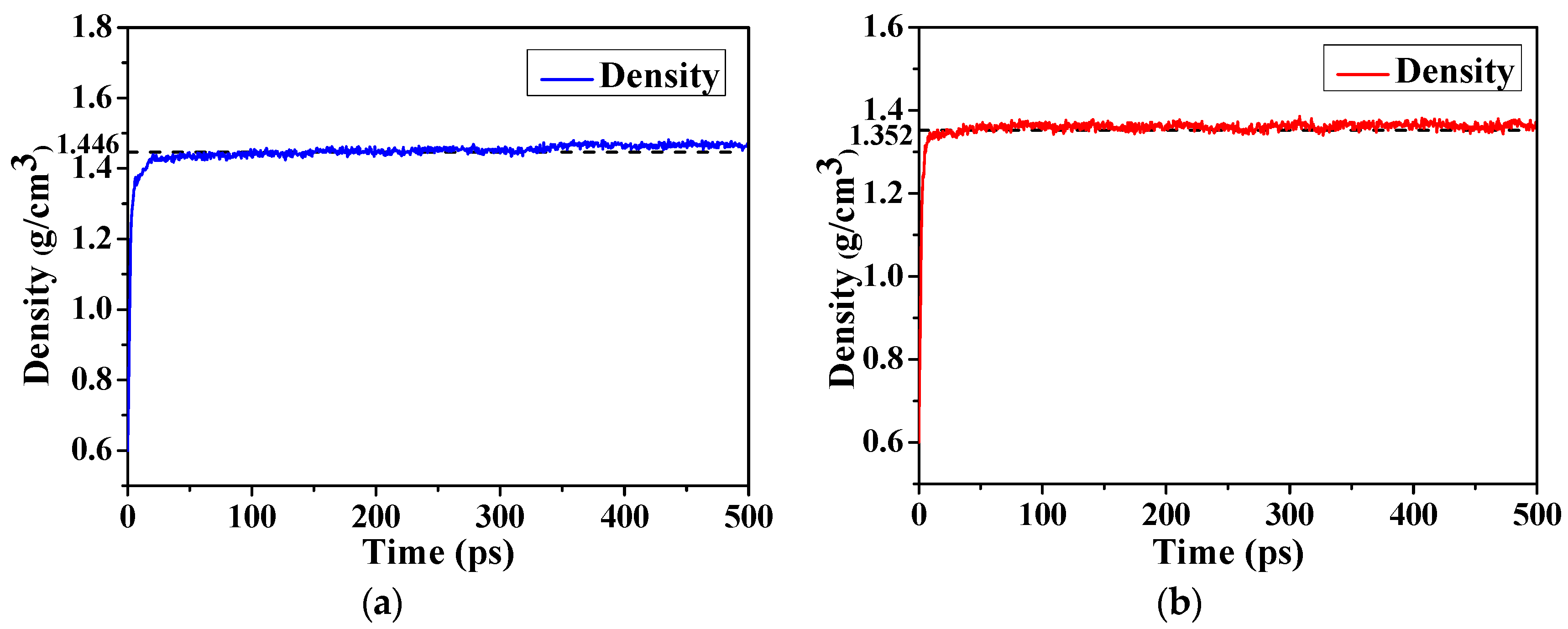
Because accidental errors can be introduced during molecular dynamics simulation, during the calculation of steady-state density, the parameter set was kept consistent, and the calculations were repeated five times to provide an average value and avoid accidental errors. The density variation of the cellulose models over time obtained using the two force fields is shown in Figure 6.
Over time, the density rapidly increased to reach a steady state for the calculations using the two force fields (Figure 6). Table 3 shows that the steady-state density of cellulose is 1.446 g/cm3 using the COMPASS force field, while it is 1.352 g/cm3 using the PCFF force field. The density of cellulose specified in the Polymer Handbook is 1.480 g/cm3 [33], so the steady-state density of cellulose obtained in the COMPASS force field is closer to the actual density of cellulose than that obtained with the PCFF. The properties of cellulose can be reflected more accurately by using the COMPASS force field than that using the PCFF force field. Therefore, the COMPASS force field is better than the PCFF in the molecular dynamics simulation of cellulose.
3.3. Analysis of Repeatability and Volatility
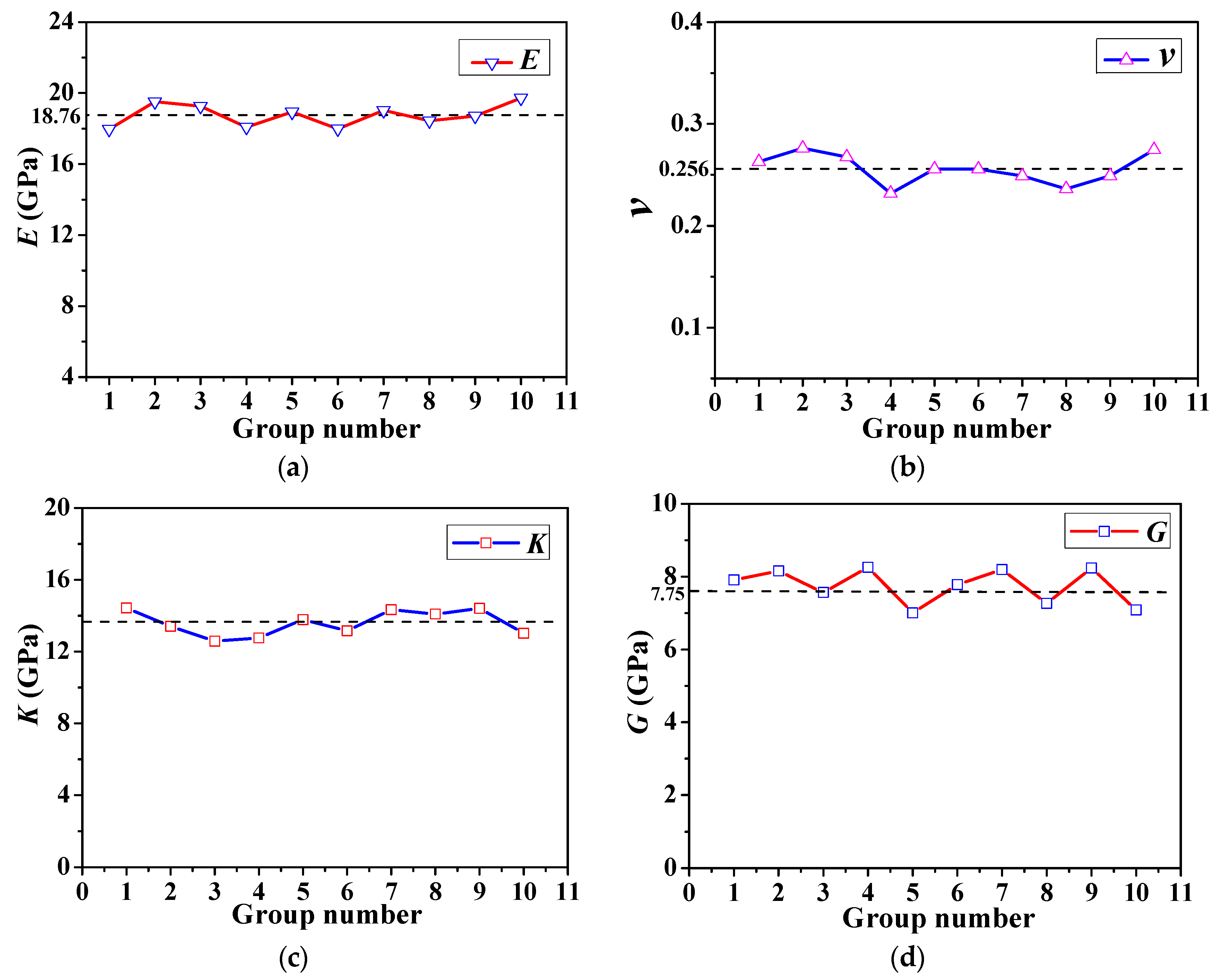
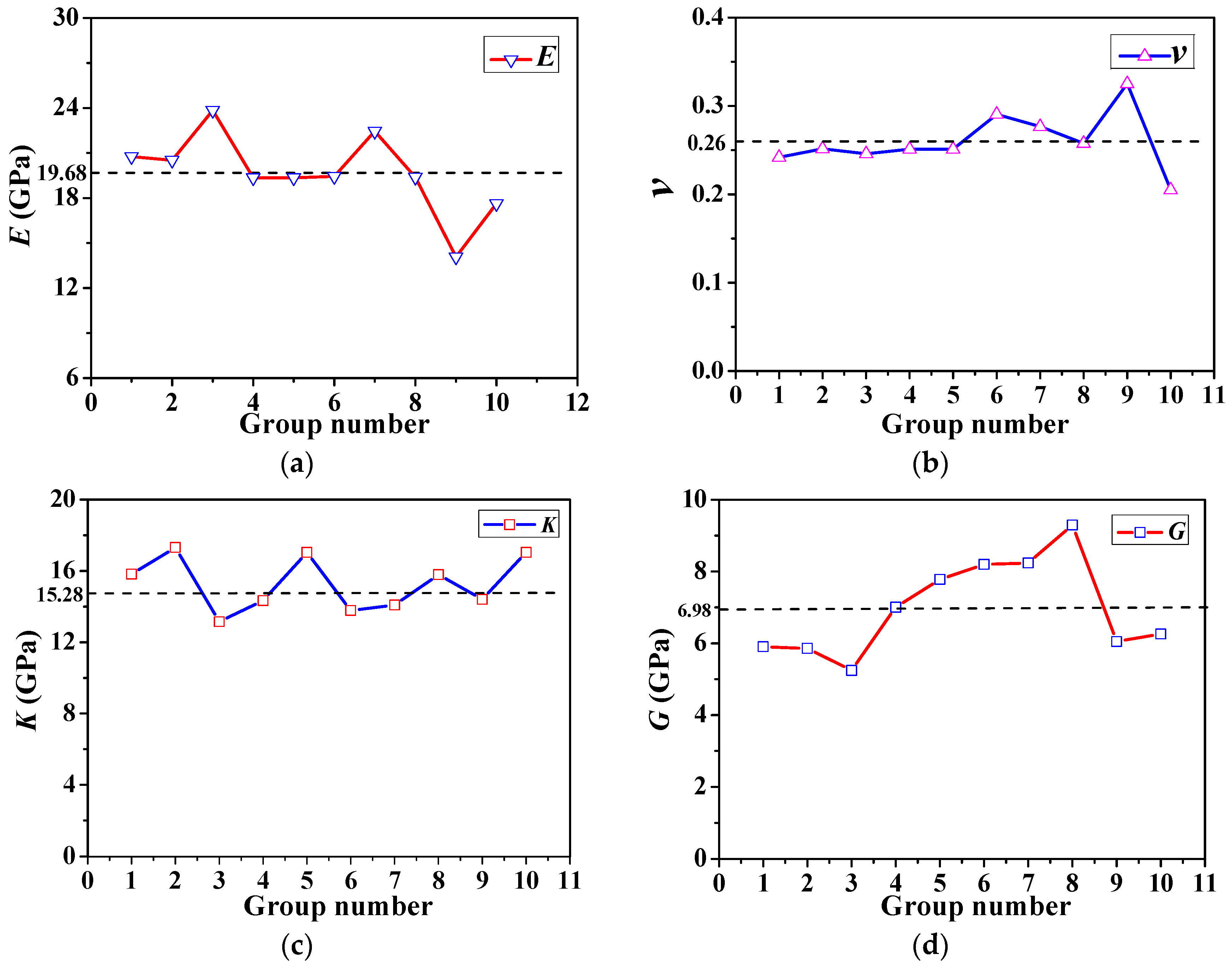
In this paper, 10 groups of data were repeatedly simulated, and the better force field was obtained through comparison of the volatility and repeatability of the mechanical properties of the model calculated using the two force fields. The changes of the calculated values of E, v, K, and G for the 10 groups using the COMPASS force field are presented in Figure 7, while those obtained with the PCFF force field are shown in Figure 8.
The average values (μ), standard deviations (s), and maximum deviation factors (β) for the data for the 10 groups for each force field were determined. The average value reflects the centrotaxis of the data. The standard deviation represents the discreteness of the data, which can be used to indicate the degree of dispersion, and a large standard deviation means a greater degree of discretization. The maximum deviation factor is the absolute difference between the maximum (minimum) sample value and average value divided by the average value. The average value, standard deviation, and maximum deviation factor of E and v for the data for the 10 groups for each force field are presented in Table 4.
From a qualitative point of view, Figure 7 and Figure 8 shows that the values of the volatility of E, v, K, and G under the COMPASS force field are obviously less than those under the PCFF force field. Table 4 reveals that E obtained from the two force fields is similar to Reference [29]. However, the standard deviation (s) of E and v obtained using the COMPASS force field is obviously smaller than that with the PCFF force field. This indicates that the discreteness of the mechanical properties of the model is better and the data are more concentrated using the COMPASS force field than using the PCFF one. Additionally, the maximum deviation factors (β) of E, v, K, and G using the COMPASS force field are obviously smaller than those obtained using the PCFF force field. This indicates that the fluctuation range of the mechanical properties of the model is smaller and the volatility is lower using the COMPASS force field rather than the PCFF. Thus, it is better to choose the COMPASS force field for cellulose molecular dynamics simulation than the PCFF force field.
4. Conclusions
The range of the polymerization degree used in the calculation models of cellulose was determined through analysis of the variation of the mechanical properties and the solubility of the cellulose chains with increasing DP. The optimal force field was obtained using a stable polymerization degree of the model to compare the two force fields. The agreement between the steady-state densities calculated for the models with the two force fields and the actual density of cellulose was investigated. The volatility and repeatability of the mechanical properties determined for the models with two different force fields were determined. The following conclusions were drawn:
- (1)
- When the DP of the model was less than 10, the model is inconsistent with the polysaccharide properties of cellulose. When DP exceeded 10, the results conformed to the actual mechanical and chemical properties of cellulose. Therefore, the polymerization degree of the model constructed for molecular dynamics simulation of cellulose should not be less than 10.
- (2)
- The steady-state density of cellulose obtained using the COMPASS force field was closer to the actual density of cellulose than that determined using the PCFF force field. Analysis from the perspectives of repeatability and volatility revealed that good discreteness of the mechanical properties of the model, concentrated data, and small volatility were obtained using the COMPASS force field. Therefore, the COMPASS force field is better than the PCFF force field for cellulose molecular dynamics simulation.
Acknowledgments
The authors wish to thank the National Key R&D Program of China (Grant No. 2017YFB0902700, 2017YBF0902702) and the Fundamental Research Funds for the Central Universities (Grant No. XDJK2014B031) for their financial support.
Author Contributions
Xiaobo Wang and Chao Tang conceived and designed the simulations; Qian Wang, Xiaoping Li, and Jian Hao performed the simulations; all authors analyzed the data; Xiaobo Wang and Chao Tang wrote the paper, while other authors offered their modification suggestions for the manuscript.
Conflicts of Interest
The authors declare no conflict of interest.
References
- Wang, X.; Xiao, S.B.; Zhang, Z.L.; He, J.Y. Effect of Nanoparticles on Spontaneous Imbibition of Water into Ultraconfined Reservoir Capillary by Molecular Dynamics Simulation. Energies 2017, 10, 506. [Google Scholar] [CrossRef]
- Niall, J. Massively-Parallel Molecular Dynamics Simulation of Clathrate Hydrates on Blue Gene Platforms. Energies 2013, 6, 3072–3081. [Google Scholar]
- Han, H.H. Research on Transformer Aging Character and Analysis Aging Mechanism. Ph.D. Thesis, Changsha University of Science and Technology, Changsha, China, 2010. [Google Scholar]
- Lu, X.; Han, S.; Li, Q.M.; Wang, X.L.; Wang, G.Y. Reactive Molecular Dynamics Simulation of Polyimide Pyrolysis Mechanism at High Temperature. Trans. China. Electrotech. Soc. 2016, 31, 15–20. [Google Scholar]
- Deng, S.W.; Huang, Y.M.; Liu, H.L.; Hu, Y. Computer Simulation of Mechanical Properties of Polymer Materials. CIESC J. 2015, 66, 2768–2770. [Google Scholar]
- Miyamoto, H.; Rein, D.; Ueda, K.; Yamane, C.; Cohen, Y. Molecular Dynamics Simulation of Cellulose-coated Oil-in-water Emulsions. Cellulose 2017, 24, 2699–2711. [Google Scholar] [CrossRef]
- Reid, M.; Villalobos, M.; Cranston, E. The Role of Hydrogen Bonding in Non-ionic Polymer Adsorption to Cellulose Nanocrystals and Silica Colloids. Curr. Opin. Colloid Interface Sci. 2017, 29, 76–82. [Google Scholar] [CrossRef]
- Tang, C.; Zhang, S.; Wang, Q.; Wang, X.B.; Hao, J. Thermal Stability of Modified Insulation Paper Cellulose Based on Molecular Dynamics Simulation. Energies 2017, 10, 397. [Google Scholar] [CrossRef]
- Kono, H.; Ogasawara, K.; Kusumoto, R.; Oshima, K.; Hashimoto, H.; Shimizu, Y. Cationic Cellulose Hydrogels Cross-linked by Poly(ethylene glycol): Preparation, Molecular Dynamics, and Adsorption of Anionic Dyes. Carbohydr. Polym. 2016, 152, 170–180. [Google Scholar] [CrossRef] [PubMed]
- Berglund, J.; Angles, D.; Vilaplana, F. A Molecular Dynamics Study of the Effect of Glycosidic Linkage Type in the Hemicellulose Backbone on the Molecular Chain Flexibility. Plant J. 2016, 88, 56–70. [Google Scholar] [CrossRef] [PubMed]
- Mazeau, K.; Heux, L. Molecular Dynamics Simulations of Bulk Native Crystalline and Amorphous Structures of Cellulose. J. Phys. Chem. B 2003, 107, 2394–2403. [Google Scholar] [CrossRef]
- Paajanen, A.; Vaari, J. High-temperature Decomposition of the Cellulose Molecule: A Stochastic Molecular Dynamics Study. Cellulose 2017, 24, 2713–2725. [Google Scholar] [CrossRef]
- Zhu, M.Z. Molecular Dynamics Study of Thermal Aging of Oil-impregnated Insulation Paper. Ph.D. Thesis, Chongqing University, Chongqing, China, 2012. [Google Scholar]
- Zhang, X.M.; Mark, A. Mechanical Properties of Amorphous Cellulose Using Molecular Dynamics Simulations with a Reactive Force Field. Int. J. Model. Identif. Control 2013, 18, 211–217. [Google Scholar] [CrossRef]
- Matthews, J.F.; Bergenstrahle, M.; Wohlert, J.; Brady, J.W.; Himmel, M.E.; Crowley, M.F. Simulations of Cellulose Microfibrils with Several Molecular Mechanics Force Fields; American Chemical Society: Washington, DC, USA, 2010. [Google Scholar]
- Mostofian, B.; Cheng, X.; Smith, J.C. Replica-exchange Molecular Dynamics Simulations of Cellulose Solvated in Water and in the Ionic Liquid 1-butyl-3-methylimidazolium Chloride. J. Phys. Chem. B 2014, 118, 11037–11049. [Google Scholar] [CrossRef] [PubMed]
- Liu, C.; Jiang, D.Z.; Wei, S.A.; Huang, J.B. A Study of Thermal Decomposition in Cellulose by Molecular Dynamics Simulation. Nat. Sci. 2009, 1, 41–46. [Google Scholar] [CrossRef]
- Huang, J.B.; Liu, C.; Wei, S.A.; Fan, X.; Jiang, D.Z. Molecular Simulation of Pyrolysis Mechanism of Cellulose and Analysis of Formation Paths of Major Products. J. Chongqing Univ. 2010, 33, 65–69. [Google Scholar]
- Huang, R.; Yao, W.S.; Tan, H.M. Molecular Simulation of Cellulose-based Energetic Binders. Chin. J. Explos. Propellants 2008, 31, 64–67. [Google Scholar]
- Zhang, X.M.; Shi, S.Q.; Cao, J. Elastic Properties of Cellulose by Molecular Dynamics Simulation. Appl. Mech. Mater. 2013, 416–417, 1726–1730. [Google Scholar] [CrossRef]
- Chen, W.; Lickfield, G.C.; Yang, C.Q. Molecular modeling of cellulose in amorphous state. Part I: Model building and plastic deformation study. Polymer 2004, 45, 1063–1071. [Google Scholar] [CrossRef]
- Bazooyar, F.; Momany, F.A.; Bolton, K. Validating Empirical Force Fields for Molecular-level Simulation of Cellulose Dissolution. Comput. Theor. Chem. 2012, 984, 119–127. [Google Scholar] [CrossRef]
- Berendsen, H.J.C.; Postma, J.P.M.; Funsteren, W.F. Molecular dynamics with coupling to an external bath. J. Chem. Phys. 1984, 81, 3684–3690. [Google Scholar] [CrossRef]
- Andrea, T.A.; Swope, W.C.; Andersen, H.C. The role of long ranged forces in determining the structure and properties of liquid water. J. Chem. Phys. 1983, 79, 4576–4584. [Google Scholar] [CrossRef]
- Lu, Y.C. The Aging Mechanism and Gas Diffusion Behavior Research in Molecular Simulation of Oil Paper Insulation. Ph.D. Thesis, Chongqing University, Chongqing, China, 2007. [Google Scholar]
- Zhang, S.; Tang, C.; Wang, X.B.; Hao, J. Thermal stability and dielectric property of nano-SiO2-doped cellulose. Appl. Phys. Lett. 2017, 111, 012902. [Google Scholar] [CrossRef]
- Liao, R.J.; Zhu, M.Z.; Yang, L.J. Molecular dynamics study of water molecule diffusion in oil-paper insulation materials. Phys. B Condens. Matter 2011, 406, 1162–1168. [Google Scholar] [CrossRef]
- Liao, R.J.; Zhang, F.Z.; Yuan, Y. Preparation of a dicyandiamide contained novel insulation paper and an experiment on the thermal aging characteristics of reel oil-paper insulations. J. Chongqing Univ. 2013, 36, 47–51. [Google Scholar]
- Nie, S.J. Molecular Simulation Study on Oxidation and Hydrolysis of Amorphous Region of Cellulosic Insulation Paper in Power Transformer. Ph.D. Thesis, Chongqing University, Chongqing, China, 2013. [Google Scholar]
- Tang, C.; Zhang, S.; Li, X. Molecular dynamics simulations of the effect of shape and size of SiO2 nanoparticle dopants on insulation paper cellulose. AIP Adv. 2016, 6, 125106. [Google Scholar] [CrossRef]
- Hak, L.L.; Philip, L. The Solubility Parameter of Cellulose and Alkylketene Dimer (AKD) Determined by Inverse Gas Chromatography. J. Wood Chem. Technol. 1991, 45, 1063–1071. [Google Scholar]
- Rowe, R.C. The prediction of compatibility/incompatibility in blends of ethyl cellulose with hydroxypropyl methylcellulose or hydroxypropyl cellulose using 2-dimensional solubility parameter maps. J. Pharm. Pharmacol. 1986, 38, 214–215. [Google Scholar] [CrossRef] [PubMed]
- Mark, H.F. Encyclopedia of Polymer Science and Technology, 2nd ed.; John Wiley & Sons, Inc.: New York, NY, USA, 1982; pp. 35–68. [Google Scholar]
Figure 1.
Models in the amorphous region of cellulose with DP of 10 calculated using (a) the COMPASS force field and (b) the PCFF force field.
Figure 1.
Models in the amorphous region of cellulose with DP of 10 calculated using (a) the COMPASS force field and (b) the PCFF force field.
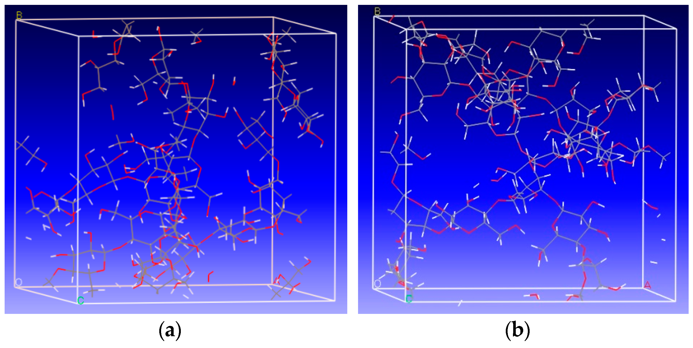
Figure 2.
Changes of (a) the tensile modulus (E) and (b) the shear modulus (G) with DP simulated using the COMPASS force field.
Figure 2.
Changes of (a) the tensile modulus (E) and (b) the shear modulus (G) with DP simulated using the COMPASS force field.
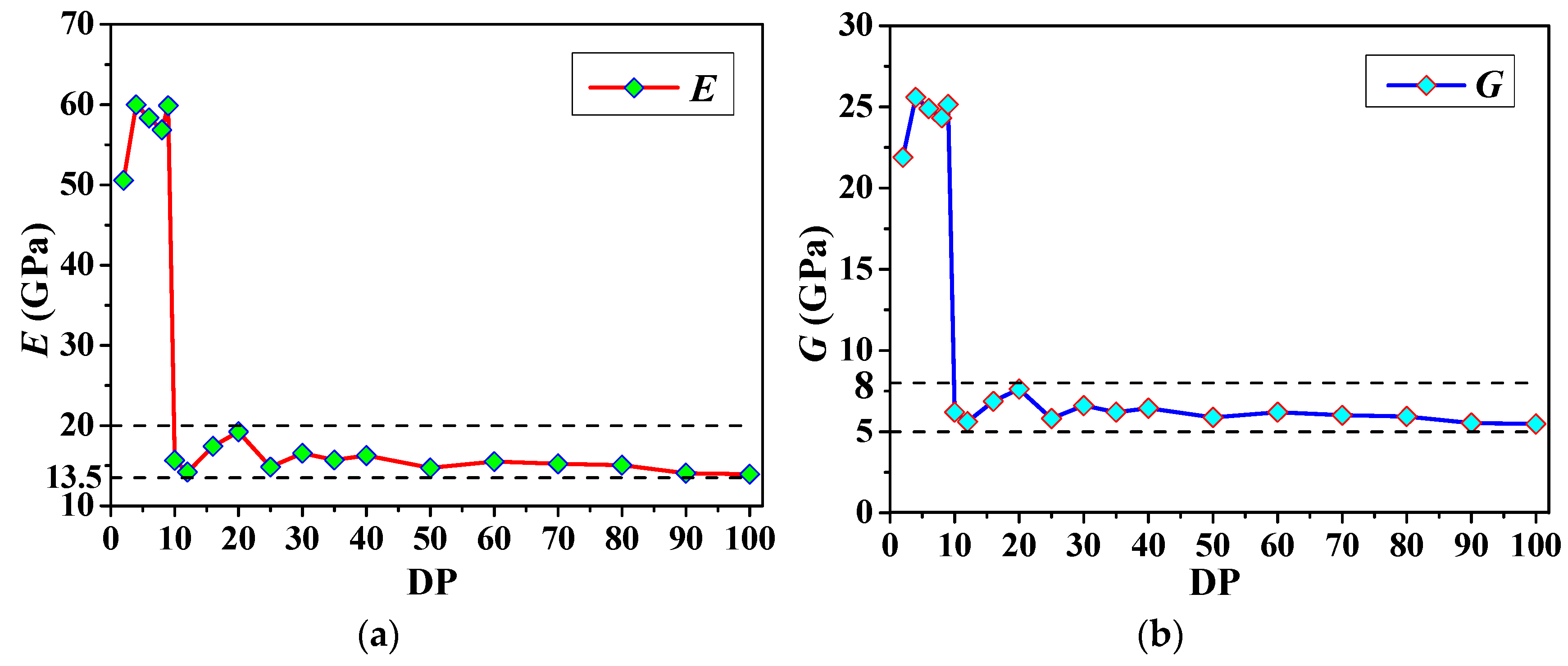
Figure 3.
Changes of (a) the tensile modulus (E) and (b) the shear modulus (G) with DP simulated using the PCFF force field.
Figure 3.
Changes of (a) the tensile modulus (E) and (b) the shear modulus (G) with DP simulated using the PCFF force field.

Figure 4.
Structure of a cellulose chain.

Figure 5.
Dependence of CED on DP calculated using (a) the COMPASS force field and (b) the PCFF force field.
Figure 5.
Dependence of CED on DP calculated using (a) the COMPASS force field and (b) the PCFF force field.

Figure 6.
Density variation over time calculated using (a) the COMPASS force field and (b) the PCFF force field.
Figure 6.
Density variation over time calculated using (a) the COMPASS force field and (b) the PCFF force field.

Figure 7.
Changes of (a) the tensile modulus (E), (b) the Poisson’s ratio (v), (c) the bulk modulus (K) and (d) the shear modulus (G) of 10 groups of repeated simulation calculated using the COMPASS force field.
Figure 7.
Changes of (a) the tensile modulus (E), (b) the Poisson’s ratio (v), (c) the bulk modulus (K) and (d) the shear modulus (G) of 10 groups of repeated simulation calculated using the COMPASS force field.

Figure 8.
Changes of (a) the tensile modulus (E), (b) the Poisson’s ratio (v), (c) the bulk modulus (K) and (d) the shear modulus (G) of 10 groups of repeated simulation calculated using the PCFF force field.
Figure 8.
Changes of (a) the tensile modulus (E), (b) the Poisson’s ratio (v), (c) the bulk modulus (K) and (d) the shear modulus (G) of 10 groups of repeated simulation calculated using the PCFF force field.


Table 1.
Average values of E, G, v, and C12-C44 of properties in a steady state of the cellulose models using different force fields.
Table 1.
Average values of E, G, v, and C12-C44 of properties in a steady state of the cellulose models using different force fields.
| COMPASS | PCFF | ||||||
|---|---|---|---|---|---|---|---|
| E | G | v | C12-C44 | E | G | v | C12-C44 |
| 14.568 | 5.766 | 0.248 | 0.143 | 17.939 | 6.890 | 0.276 | 0.118 |
Table 2.
Average values of E, G, v, and C12-C44 calculated using different force fields.
| DP | 10 | 20 | 30 | 40 | 50 | 60 | 70 | 80 | 90 | 100 | Average |
|---|---|---|---|---|---|---|---|---|---|---|---|
| COMPASS | 26.4 | 25.6 | 25.3 | 25.4 | 24.9 | 25.5 | 25.2 | 25.6 | 24.6 | 25.2 | 25.4 |
| PCFF | 28.4 | 28.1 | 28.7 | 28.4 | 28.5 | 28.2 | 28.3 | 28.2 | 28.5 | 28.3 | 28.4 |
Table 3.
Average values of E, G, v, and C12-C44 calculated using different force fields.
| COMPASS | PCFF | ||||||||||
|---|---|---|---|---|---|---|---|---|---|---|---|
| 1 | 2 | 3 | 4 | 5 | Average | 1 | 2 | 3 | 4 | 5 | Average |
| 1.41 | 1.43 | 1.47 | 1.47 | 1.45 | 1.446 | 1.36 | 1.34 | 1.35 | 1.31 | 1.40 | 1.352 |
Table 4.
Average value, standard deviation, and maximum deviation factor of E and v calculated using COMPASS and PCFF force fields.
Table 4.
Average value, standard deviation, and maximum deviation factor of E and v calculated using COMPASS and PCFF force fields.
| COMPASS | PCFF | |||||
|---|---|---|---|---|---|---|
| Parameter | μ | s | β (%) | μ | s | β (%) |
| E | 18.76 | 0.64 | 5.09 | 19.68 | 2.64 | 21.15 |
| v | 0.26 | 0.01 | 9.39 | 0.26 | 0.03 | 25.25 |
© 2017 by the authors. Licensee MDPI, Basel, Switzerland. This article is an open access article distributed under the terms and conditions of the Creative Commons Attribution (CC BY) license (http://creativecommons.org/licenses/by/4.0/).
Share and Cite
MDPI and ACS Style
Wang, X.; Tang, C.; Wang, Q.; Li, X.; Hao, J. Selection of Optimal Polymerization Degree and Force Field in the Molecular Dynamics Simulation of Insulating Paper Cellulose. Energies 2017, 10, 1377. https://doi.org/10.3390/en10091377
AMA Style
Wang X, Tang C, Wang Q, Li X, Hao J. Selection of Optimal Polymerization Degree and Force Field in the Molecular Dynamics Simulation of Insulating Paper Cellulose. Energies. 2017; 10(9):1377. https://doi.org/10.3390/en10091377
Chicago/Turabian StyleWang, Xiaobo, Chao Tang, Qian Wang, Xiaoping Li, and Jian Hao. 2017. "Selection of Optimal Polymerization Degree and Force Field in the Molecular Dynamics Simulation of Insulating Paper Cellulose" Energies 10, no. 9: 1377. https://doi.org/10.3390/en10091377
Note that from the first issue of 2016, this journal uses article numbers instead of page numbers. See further details here.