Transmission Expansion Planning Using TLBO Algorithm in the Presence of Demand Response Resources

Tehran Polytechnic, Amirkabir University of Technology, 424 Hafez Ave, 159163-4311 Tehran, Iran
*
Author to whom correspondence should be addressed.
Energies 2017, 10(9), 1376; https://doi.org/10.3390/en10091376
Submission received: 11 July 2017
/
Revised: 4 September 2017
/
Accepted: 5 September 2017
/
Published: 11 September 2017
(This article belongs to the Section F: Electrical Engineering)
Abstract
:Transmission Expansion Planning (TEP) involves determining if and how transmission lines should be added to the power grid so that the operational and investment costs are minimized. TEP is a major issue in smart grid development, where demand response resources affect short- and long-term power system decisions, and these in turn, affect TEP. First, this paper discusses the effects of demand response programs on reducing the final costs of a system in TEP. Then, the TEP problem is solved using a Teaching Learning Based Optimization (TLBO) algorithm taking into consideration power generation costs, power loss, and line construction costs. Simulation results show the optimal effect of demand response programs on postponing the additional cost of investments for supplying peak load.
1. Introduction
Installing new devices on an existing power system while ensuring stability and reliability of the power system are the main goals of Transmission Expansion Planning (TEP). This planning is based on load prediction and power supply conditions. From a mathematical view point, TEP is a nonlinear, discrete, and large-scale optimization problem with many equality and inequality constraints. Transmission line planning can be divided into evolutionary, mathematical, and meta-heuristic methods.
The evolutionary method quickly converges to the optimal solution, but for a large scale and complex problem, it can converge to a solution that is far from ideal. One of the first methods for solving the expansion transmission network problem was presented in 1970 by Garver [1]. In this work, the problem is formulated as a load distribution problem; the objective function and the constraints are described by linear functions that neglect Ohmic power loss. Considering the newly added lines, new linear load flow is calculated, and the operation continues until no overload exists in the system. Lattore et al. proposed an evolutionary method in which the transmission line is decomposed into two problems: generation and investment [2]. The investment problem is solved by an evolutionary method, while the generation problem is solved by a known optimization method. In prior studies [3,4,5,6,7,8,9,10,11], researchers have solved the same problem using the evolutionary method by sensitivity analysis. In each step of the algorithm, the sensitivity index is used for determining the added circuits (lines). The sensitivity index can be generated based on the algorithm implemented in an electrical system like minimum depletion [3], load feeding [4], lowest criteria [6], a lighter version of its own mathematical model [5,7,8], or the optimal load flow [9,10]. In most models, the internal point method is used for solving the linear or non-linear planning problem in each iteration.
One of the first mathematical optimization methods for solving the transmission network expansion is the linear planning technique, in which both the constraints and the objective function are linear [12,13]. The linear TEP problem is decomposed into two independent investment and generation problems, which are defined by a linear planning model and Monte Carlo, respectively, based on DC load flow. Nonlinear planning is another mathematical planning tool used to address the TEP problem [14]. In this method, the objective function and some constraints are formulated as nonlinear equations. The objective function considers minimizing the investment costs, Ohmic losses, and corona. The main drawback of this method is that the optimal solution may get stuck in the local optimal point, and problems are associated with the determination of the initial values of an unknown load flow. Another optimization method for solving the transmission line expansion is mathematical decomposition, which is one of the first methods formulated by Pereira et al. [15]. In [16], a multistage decomposition scheme based on Nested Benders decomposition was applied to the TEP problem. A two-phase bounding and decomposition approach, to compute optimal and near-optimal solutions to large-scale mixed-integer investment planning problems, was proposed by Falugi et al. [17].
Jingdong and Guoqing [18] implemented a genetic algorithm (GA) as the objective function in order to use heuristic methods to combine the features of evolutionary and mathematical methods. One of the first methods implemented for solving the TEP problem was the genetic algorithm [18,19]. The GA method is based on evaluating the TEP Multi-Objective Programming, while considering the minimum investment cost, the optimal system reliability, and minimizing the effect on the environment. Silva et al. proposed a report on applying the GA to the TEP optimization problem, in which the principle of simulated annealing (SA) was applied to improve the unique mechanism of evolution and generation [19]. A combination of GA and neurocomputing was used by Yoshimoto et al. [20] that can be more effective in solving TEP problems. A parallel SA algorithm was implemented by Gallego et al. [21] that significantly reduced the computation burden and improved quality of the SA solution. A new static TEP solution, based on the Tabu search application, was developed by Wen et al. [22]. In this paper, the transmission network planning problem is developed as a one and zero integer number planning, based on a Tabu search method. Furthermore, a Tabu search method, including phase amplification and a variety of concepts, was reported by Wen and Chang [22]. A greedy randomization adaptive search procedure was proposed by Binato et al. [23]. Maghouli et al. [24] presented a multi-stage transmission expansion method, using a multi-objective optimization framework with internal scenario analysis for handling uncertainties. Maghouli et al. [25] also developed a multi-objective TEP methodology in a deregulated power system with the presence of wind generation, considering investment cost, use of private investment, and reliability of the system as the objective functions.
Demand response programs (DRPs) are effective in decision-making policies in power systems. Postponing additional investment costs for supplying the peak load, which occurs only for a few hours in a year, is the advantage of using DRPs while studying power system planning. Applying DRPs affects long- and short-term decision-making policies for a power system. Therefore, implementing DRPs in transmission line expansion planning can be useful [26,27,28]. In [29], an economic analysis of TEP was introduced using Successive Linear Programming while considering demand response resources. The results of the method presented in [29] show that a demand response program can significantly reduce generation operating and investment costs. Another method for TEP under generation uncertainty was proposed by Konstantelos and Strbac [30], where the potential for flexible network technologies, such as phase-shifting transformers, and non-network solutions, such as energy storage and demand-side management, were assessed.
In this paper, we attempted to reduce the overall costs of the system and postpone the additional cost of constructing new lines, due to just a few peak load occurrences in a year, by implementing an incentive-based demand response program through investment in these programs. Then, a meta-heuristic method is used for transmission expansion planning using the Teaching Learning Based Optimization (TLBO) algorithm. The proposed method was implemented on the IEEE six-bus and 57-bus networks. The proposed method can be considered as a bi-level problem. On the first level, an incentive-based demand response program was implemented for peak load reduction and, in turn, reduction of TEP costs. This method can be considered similar to integrating Distributed Generations (DGs) or installing Flexible Alternating Current Transmission System (FACTS) devices in the system, in order to reduce TEP costs. On the second level, the TEP problem was solved using the TLBO algorithm so that the costs of generation, losses, and lines were minimized. By reducing the load peak in the first level, fewer lines are required in the TEP program, resulting in lower total costs while the profit of demand response is maintained. A schematic diagram of the proposed method is shown in Figure 1. According to this Figure, after implementing DRP and TEP, the total cost is calculated. If the total cost of DRP and TEP objective function was less than the cost of normal operation of the network (Before DRP and TEP), DRP is applied in a way that customer participation in DRP is reduced. This can be done by reducing the incentive price or increasing the limitations of customer participation in DRP. In summary, our contribution is as follows:
- (1)
- Evaluation of the influence of an incentive-based DRP on TEP.
- (2)
- Developing TEP as a nonlinear function of the costs of losses, generation, and line construction.
- (3)
- Application of TLBO as a robust meta-heuristic algorithm for minimizing the TEP total costs.
In the following sections, DRP modelling, TLBO algorithm, TEP formulation, simulation results, and conclusion are described.
2. Modelling the Demand Response Program
In order to formulate the customer’s contribution to a DRP, an economic load model was developed which proposes a variation in the customer’s demands related to the change in electricity prices, incentives, and penalties for customers [31].
2.1. Elasticity in Demand Price
Elasticity is defined as the demand sensitivity in relation to the price [32]:
According to Equation (1), the elasticity price of the ith period versus jth period is:
If the electricity price is different for various periods, the demand will respond as one of the following [33]. Some loads cannot be shifted from one period to another, for example light loads, and they can be on or off. Therefore, these loads are sensitive in a single period which is known as “self-elasticity”, which is always a negative value. Some of the costs can be shifted from one peak period to off-peak or low periods, for example, process loads. This behavior is called multi-period sensitivity and is known as “cross-elasticity”, which is always a positive value. Therefore, for a 24-h period, the elasticity coefficients can be arranged in a 24-by-24 matrix as follows:
The diagonal elements in the matrix show the self-elasticity, and the non-diagonal elements correspond to the cross-elasticity. Column j shows how a price change during the single period j will affect demands in all periods. Calculation of elasticity has been described in more details [34]. According to Moghaddam et al. [34], if a linear function , where and are the coefficients of linear demand curve, is considered as a mathematical function for representing a downward sloping price (P) versus demand (d), the self-elasticity can be represented as follows [34]:
Moreover, if it is assumed the electricity market offers electricity in three different price categories as P(i), P(j) and P(k) for valley, off-peak, and peak periods, respectively, the cross elasticity can be represented as follows [34]:
2.2. Modeling Single Period Elastic Loads
Consider that the customer changes his demand from do(t) (initial demand) to d(i), based on the incentives and penalties indicated in the contracts:
If A(i) $ is given to the customer for each kWh load reduction per ith hour as an incentive, the total incentive for the company would be as follows:
If the customer who enrolled in DRPs does not commit to the obligations mentioned in the contract, they will be penalized. If the contract level for ith hour and the penalty for the same period are shown by IC(i) and pen(i), respectively, the total penalty is calculated as follows:
Considering B(d(i)) as the user earning at the ith hour due to using d(i) kWh electrical energy, the profit of customer, S, for the ith hour is:
Based on the classic optimization rules, must be zero in order to maximize the customer profit.
The profit function commonly used is a quadratic function:
By differentiating the above equation and the solution for and replacing into Equation (9), we will have:
Therefore, user consumption will be:
2.3. Modeling Multi-Period Elastic Loads
Based on the definition of cross-elasticity in Equation (2) and considering the linearity as follows:
The linear relation between price and demand is:
If the incentive and penalty are replaced in the price equation, the multi-period model will be as follows:
2.4. Economic Load Model
Comparing Equations (14) and (17) results in the following responsive economic load model:
The above equation shows how much profit is required to maximize the profit in a 24-h period while participating in DRPs.
3. TLBO Algorithm
The TLBO algorithm is a population-based method that simulates the behavior of the teacher and students so as to increase the class level [35]. The teacher and students are the main components of this method. The students increase their level in two steps: the teacher step, in which the teacher tries to increase the class level, and the student step, in which students increase their scores through interaction amongst themselves. The most knowledgeable student, which is the best answer, is called the teacher. The TLBO process is divided into two stages which are explained below.
3.1. Teacher Step
As explained before, the best answer is considered the teacher. The teacher tries to increase the student class level, for example (Mi) to his own level (MT). However, this is not possible in practice. So, the teacher tries to increase the average level of the class (Mmean) to a higher level, for example M2. Obviously, a good teacher, a more suitable answer, performs better for the students. To explain the teacher step, the difference between MT and Mmean is estimated as:
where ri is a random variable in [0, 1], and Tf is the teacher factor between 1 and 2. Based on differ_mean, the answer will be updated as follows:
3.2. Student Step
A student can share his knowledge with another student selected randomly from the class. If the second student has more knowledge, the first one will learn new things; otherwise, the second one will learn. In order to formulate this process, let Xi and Xj be these two students and i ≠ j. Xi is updated using the following equations:
In each step, Xold is replaced by Xnew if the result is better. The process is continued until the convergence conditions are achieved. The TLBO flowchart is shown in Figure 2.
In this paper, TLBO is chosen for minimizing the TEP problem due to some reasons. First, TLBO is introduced as a strong algorithm in converging to the global optimum which is superior to some other heuristic methods as indicated in [35]. However, the authors have run TLBO algorithm 100 times and chosen the best answers in order to make sure that it converges to the optimum answer. Second, unlike most of the heuristic algorithms, TLBO is a parameter free algorithm [35]. In TLBO algorithm, ri and Tf are the only parameters of the method which are not tuned. In other words, these parameters are selected randomly and the values of them do not influence the results of the algorithm.
4. Transmission Expansion Planning Model
In this paper, the TEP problem is formulated to minimize the generation cost while considering the line and loss costs. The transmission expansion planning is modeled using the following equations:
where xi is the number of circuits added to the right-of-way i; Ai is the candidate circuit cost for addition to the right-of-way i; t is the system runtime which is considered here as 4830 h [36]; B is the loss cost per kWh; ei is the number of circuits in the main base system; Ii is the electrical current in the ith circuit; Ri is the resistance of ith circuit; m is the right-of-way allowed to be the added line; m0 is right-of-way not allowed to be the added line; ai, bi, and ci are the cost coefficients; Pi is the active power generated from ith DG. Equation (24) is the constraint of power equation which is resulted from calculating power flow, where Pij is the active power in line i to j; and PGi and PDi are the active power generation and load on ith bus. Equation (25) is the constraint of overload that can be introduced as a penalty for the overload of each circuit, where Pimax is the maximum active power flow in ith circuit. Equation (26) is the upper and lower constraint of the number of circuits that can be added to right-of-way i.
5. Study of the Network and Simulation Results
The network studied was a Wollenberg 6-bus network, shown in Figure 3. The network data can be found in [37].
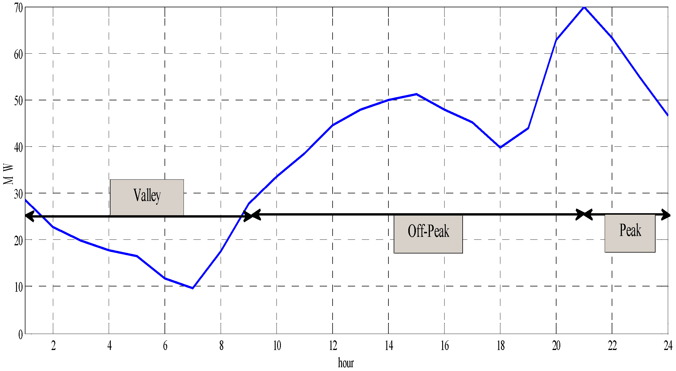
Buses four and six were considered to be responsive, and the maximum number of lines that could be added between two different buses is three. The load diagram for bus four is shown in Figure 4.
In this study, we assumed that the pattern of bus four (Iran load pattern), which is shown in Figure 4, is divided into three different regions: a valley period from 12:00 a.m. to 9:00 a.m., an off-peak period from 9:00 a.m. to 9:00 p.m., and a peak period from 9:00 p.m. to 12:00 a.m. Notably, the loads in the 24 h of a day have uncertainties with lower and upper bands. In other words, Lh∈[Ll, Lu], in which Lh is the load value at the hth hour, and Ll and Lu are the lower and upper bands, respectively. In order to handle uncertainties, we assumed that the worst situation occurs [38], in which the loads are on their upper values.
The electricity price in Iran is 150 Rials/kWh as the flat rate, 400 Rials/kWh for the peak period, 160 Rials/kWh in the off-peak period, and 40 Rials/kWh in valley periods [25]. The potential of DRP implementation is considered to be 10%, which means that the total signed contracts for customer participation in the programs are equal to 10% of the total load. Accordingly, Independent System Operator (ISO) will be able to reduce the network peak load by about 3400 MW for the peak around 9:00 p.m. in order to increase the reserve margin and reduce the possibility of load shedding. The price elasticities of the demand are listed in Table 1.
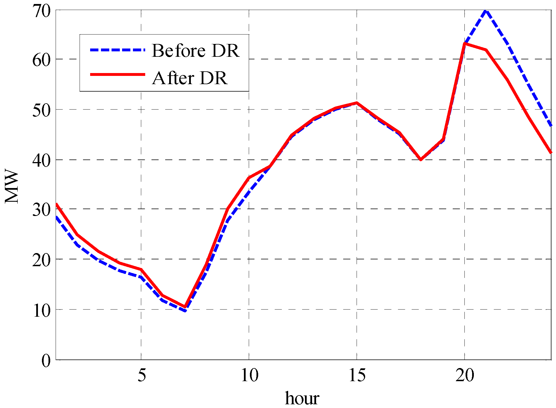
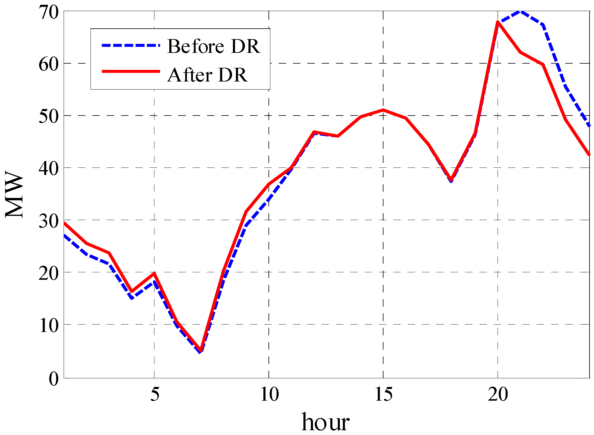
In this paper, the final costs for the system were reduced with the aid of an incentive-based demand response program. The additional cost of constructing new lines, with only a few peak load hours occurring in a year, is postponed with an incentive-based demand response program. Figure 5 and Figure 6 show 24-h loads of buses four and six, before and after the DRP.
In order to evaluate the success of the demand response program in generation and network loss costs, the two following scenarios are considered. The first scenario is performing the optimal load flow program without applying TEP, and before using the demand response program. The second scenario is performing the optimal load flow program without applying TEP and after using the demand response program.
Table 2 shows a comparison of the loss value, loss costs, generation cost, and the total cost, including difference in the losses and generation costs between the two first scenarios. Note that the cost of the loses per MWh for the intended network is 3.48 $/MWh. Based on the results in Table 2, the applied incentive-based demand response program significantly reduces the generation and loss costs, and thereby the total cost by changing load behavior. Figure 7 shows the reduction percentage of each case after implementing the DRP. According to this figure, the DRP reduces the production cost by 4.2%. Also, by using the DRP, the losses, their cost, and the total cost are reduced by 7.91%, 7.90%, and 4.26%, respectively.
After performing the demand response program, the TEP was performed. As mentioned above, the number of new lines that are allowed to be added between different buses of the intended network is three, and we assumed that this is possible for every pair of buses. By using the TLBO algorithm, transmission expansion will be done so that the objective function from Section 4 is optimized, meaning the total cost including the generation, losses, and line construction costs are minimized. Here, two other cases are considered. In the first case (scenario 3), we assumed that the line construction cost is not considered in this optimization, and the optimized objective function includes the generation and losses costs. In the second case (scenario 4), we assumed that the optimal objective function includes generation, losses, and line construction costs. The results of transmission expansion planning for the above cases are included in Table 3. In this table, the DRP cost was also considered when calculating the total costs. Moreover, since the incentives and penalties in the DRPs are applied at peak hours, the results are achieved for the peak hours. The demand response (DR) cost equals the incentive cost which is given to the customers for each kWh. For calculating the hourly DR costs in peak hours from 9:00 p.m. to 12:00 a.m., the average DR cost for this period is calculated as follows:
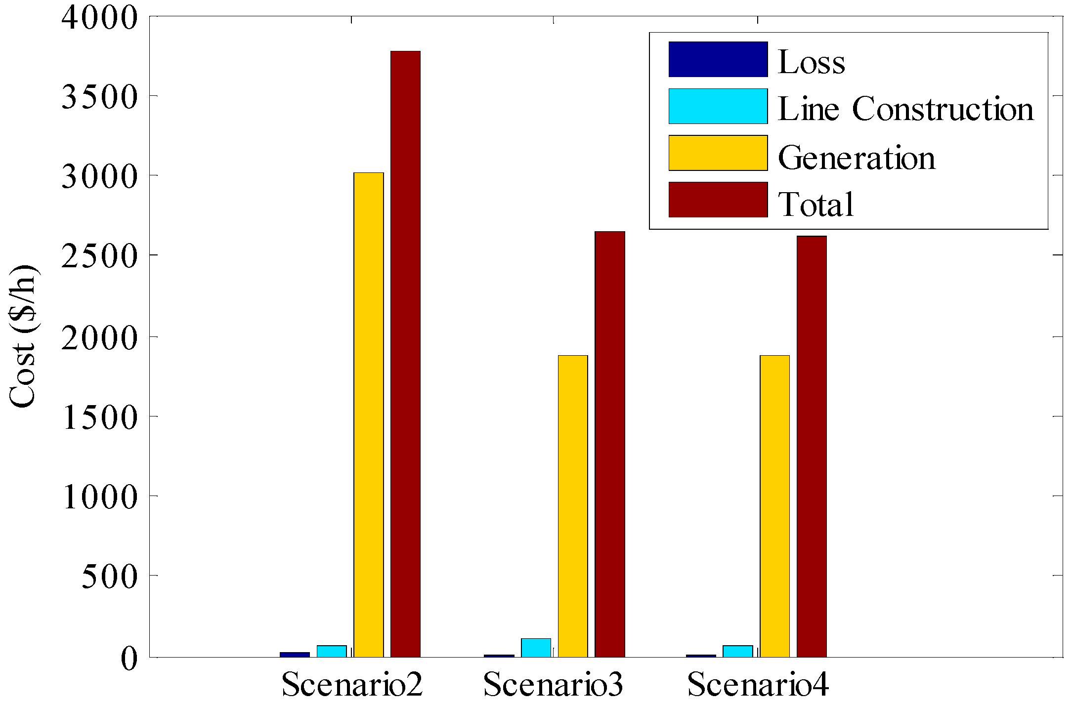
By using Equation (27), the hourly DR cost is 670.96 ($/h). According to Table 3, in scenario 3 in which the optimized objective function does not contain line construction costs, there is no limitation on the number of added lines. Therefore, by adding a large number of lines to the network, the costs and values of the losses are considerably low. However, in scenario 4, the line construction cost is considered, and hence, a few lines must be added in order to not increase the line construction cost too much. The line construction cost in this scenario is much less than in scenario 3, but the values and costs of the losses are higher. A comparison of generation, losses, and line construction costs between scenarios 2, 3, and 4 is demonstrated in Figure 8. Note that in this figure, the total cost for scenario 2 is calculated considering the demand response cost. Based on this figure and Table 2 and Table 3, we observed that in scenario 4, which includes all three costs of generation, losses, and line construction, the total cost is considerably lower.
The IEEE 57-bus network was also considered in order to evaluate the results of the TLBO algorithm. The network data can be found in [39]. We considered that buses 9, 12, 16, and 18 are responsive, and that lines can be added between buses 1, 2, 3, 6, 8, 9, 12, 16, and 17. Similar to Table 3, the results of TEP for scenarios 3 and 4 are shown in Table 4. By using Equation (27), the hourly DR cost is 900 ($/h). Based on the tabulation, we observed that in scenario 4, including all three costs of generation, losses, and line construction, the total cost is lower than in scenario 3, in which the objective function excludes the line construction cost.
6. Conclusions
In this article, the influence of a demand response program on reducing the costs of Transmission Expansion Planning (TEP) was studied. TEP was evaluated more comprehensively compared to previous works, and we modeled the problem as a nonlinear function of the costs of losses, generation, and line construction. The TLBO algorithm, which is among the most powerful optimization methods and does not lose its convergence in large systems, was used for minimizing the costs in TEP. The simulation results show that using the demand response program in TEP, the total costs are reduced by optimization methods, and additional investments can be postponed.
Author Contributions
Amir Sadegh Zakeri and Hossein Askarian Abyaneh contributed and prepared problem formulation. Amir Sadegh Zakeri analyzed the problem and wrote the paper.
Conflicts of Interest
The authors declare no conflict of interest.
References
- Garver, L.L. Transmission network estimation using linear programming. IEEE Trans. Power Appar. Syst. 1970, 89, 1688–1697. [Google Scholar] [CrossRef]
- Latorre-Bayona, G.; Perez-Arriaga, I.J. Chopin, a heuristic model for long term transmission expansion planning. IEEE Trans. Power Syst. 1994, 9, 1886–1894. [Google Scholar] [CrossRef]
- Mirhosseini, M.; Gharaveisi, A. Transmission network expansion planning with a heuristic approach. Int. J. Electron. Eng. 2010, 2, 235–237. [Google Scholar]
- Pereira, M.V.; Pinto, L.M. Application of sensitivity analysis of load supplying capability to interactive transmission expansion planning. IEEE Trans. Power Appar. Syst. 1985, 104, 381–389. [Google Scholar] [CrossRef]
- Sanchez, I.; Romero, R.; Mantovani, J.; Rider, M. Transmission-expansion planning using the dc model and nonlinear-programming technique. IEE Proc.-Gener. Transm. Distrib. 2005, 152, 763–769. [Google Scholar] [CrossRef]
- Monticelli, A.; Santos, A.; Pereira, M.; Cunha, S.; Parker, B.; Praca, J. Interactive transmission network planning using a least-effort criterion. IEEE Trans. Power Appar. Syst. 1982, 101, 3919–3925. [Google Scholar] [CrossRef]
- Sánchez, I.; Romero, R.; Mantovani, J.; Garcia, A. Interior point algorithm for linear programming used in transmission network synthesis. Electr. Power Syst. Res. 2005, 76, 9–16. [Google Scholar] [CrossRef]
- Romero, R.; Rocha, C.; Mantovani, J.; Sanchez, I. Constructive heuristic algorithm for the DC model in network transmission expansion planning. IEE Proc.-Gener. Transm. Distrib. 2005, 152, 277–282. [Google Scholar] [CrossRef]
- Rider, M.; Garcia, A.; Romero, R. Power system transmission network expansion planning using AC model. IET Gener. Transm. Distrib. 2007, 1, 731–742. [Google Scholar] [CrossRef]
- De Oliveira, E.J.; da Silva, I.; Pereira, J.L.R.; Carneiro, S. Transmission system expansion planning using a sigmoid function to handle integer investment variables. IEEE Trans. Power Syst. 2005, 20, 1616–1621. [Google Scholar] [CrossRef]
- Bennon, R.; Juves, J.; Meliopoulos, A. Use of sensitivity analysis in automated transmission planning. IEEE Trans. Power Appar. Syst. 1982, 101, 53–59. [Google Scholar] [CrossRef]
- Levi, V.; Ćalović, M. Linear-programming-based decomposition method for optimal planning of transmission network investments. IEE Proc. C Gener. Transm. Distrib. 1993, 140, 516–522. [Google Scholar] [CrossRef]
- Villasana, R.; Garver, L.; Salon, S. Transmission network planning using linear programming. IEEE Trans. Power Appar. Syst. 1985, 104, 349–356. [Google Scholar] [CrossRef]
- Al-Hamouz, Z.; Al-Faraj, A. Transmission expansion planning using nonlinear programming. In Proceedings of the Transmission and Distribution Conference and Exhibition 2002: Asia Pacific, Yokohama, Japan, 6–10 October 2002; pp. 50–55. [Google Scholar]
- Pereira, M.; Pinto, L.; Cunha, S.; Oliveira, G. A decomposition approach to automated generation/transmission expansion planning. IEEE Trans. Power Appar. Syst. 1985, 104, 3074–3083. [Google Scholar] [CrossRef]
- Munoz, F.D.; Hobbs, B.F.; Watson, J.-P. New bounding and decomposition approaches for milp investment problems: Multi-area transmission and generation planning under policy constraints. Eur. J. Oper. Res. 2016, 248, 888–898. [Google Scholar] [CrossRef]
- Falugi, P.; Konstantelos, I.; Strbac, G. Application of novel nested decomposition techniques to long-term planning problems. In Proceedings of the Power Systems Computation Conference (PSCC), Genoa, Italy, 20–24 June 2016; pp. 1–8. [Google Scholar]
- Jingdong, X.; Guoqing, T. The application of genetic algorithms in the multi-objective transmission network planning. In Proceedings of the Advances in Power System Control, Operation and Management forth International Conference, Hong Kong, China, 11–14 November 1997; pp. 338–341. [Google Scholar]
- Da Silva, E.L.; Gil, H.A.; Areiza, J.M. Transmission network expansion planning under an improved genetic algorithm. In Proceedings of the 21st 1999 IEEE International Conference on Power Industry Computer Applications, Santa Clara, CA, USA, 21 May 1999; pp. 315–321. [Google Scholar]
- Yoshimoto, K.; Yasuda, K.; Yokoyama, R. Transmission expansion planning using neuro-computing hybridized with genetic algorithm. In Proceedings of the IEEE International Conference on Evolutionary Computation, Perth, Australia, 29 November–1 December 1995; p. 126. [Google Scholar]
- Gallego, R.; Alves, A.; Monticelli, A.; Romero, R. Parallel simulated annealing applied to long term transmission network expansion planning. IEEE Trans. Power Syst. 1997, 12, 181–188. [Google Scholar] [CrossRef]
- Wen, F.; Chang, C. Transmission network optimal planning using the tabu search method. Electr. Power Syst. Res. 1997, 42, 153–163. [Google Scholar] [CrossRef]
- Binato, S.; de Oliveira, G.C.; de Araújo, J.L. A greedy randomized adaptive search procedure for transmission expansion planning. IEEE Trans. Power Syst. 2001, 16, 247–253. [Google Scholar] [CrossRef]
- Maghouli, P.; Hosseini, S.H.; Buygi, M.O.; Shahidehpour, M. A scenario-based multi-objective model for multi-stage transmission expansion planning. IEEE Trans. Power Syst. 2011, 26, 470–478. [Google Scholar] [CrossRef]
- Maghouli, P.; Hosseini, S.H.; Buygi, M.O.; Shahidehpour, M. A multi-objective framework for transmission expansion planning in deregulated environments. IEEE Trans. Power Syst. 2009, 24, 1051–1061. [Google Scholar] [CrossRef]
- Khodaei, A.; Shahidehpour, M.; Wu, L.; Li, Z. Coordination of short-term operation constraints in multi-area expansion planning. IEEE Trans. Power Syst. 2012, 27, 2242–2250. [Google Scholar] [CrossRef]
- Kazerooni, A.; Mutale, J. Transmission network planning under a price-based demand response program. In Proceedings of the 2010 IEE/PES Transmission and Distribution Conference and Exposition, New Orleans, LA, USA, 19–22 April 2010; pp. 19–22. [Google Scholar]
- Kazerooni, A.; Mutale, J. Network investment planning for high penetration of wind energy under demand response program. In Proceedings of the 2010 IEEE 11th Conference on Probabilistic Methods Applied to Power Systems (PMAPS), Singapore, 14–17 June 2010; pp. 238–243. [Google Scholar]
- Özdemir, Ö.; Munoz, F.D.; Ho, J.L.; Hobbs, B.F. Economic analysis of transmission expansion planning with price-responsive demand and quadratic losses by successive LP. IEEE Trans. Power Syst. 2016, 31, 1096–1107. [Google Scholar] [CrossRef]
- Konstantelos, I.; Strbac, G. Valuation of flexible transmission investment options under uncertainty. IEEE Trans. Power Syst. 2015, 30, 1047–1055. [Google Scholar] [CrossRef]
- Aalami, H.; Moghaddam, M.P.; Yousefi, G. Modeling and prioritizing demand response programs in power markets. Electr. Power Syst. Res. 2010, 80, 426–435. [Google Scholar] [CrossRef]
- Kirschen, D.S.; Strbac, G. Fundamentals of Power System Economics; John Wiley & Sons: Hoboken, NJ, USA, 2004. [Google Scholar]
- Buygi, M.O.; Shanechi, H.M.; Balzer, G.; Shahidehpour, M. Transmission planning approaches in restructured power systems. In Proceedings of the 2003 IEEE Bologna Power Tech Conference Proceedings, Bologna, Italy, 23–26 June 2003. [Google Scholar]
- Moghaddam, M.P.; Abdollahi, A.; Rashidinejad, M. Flexible demand response programs modeling in competitive electricity markets. Appl. Energy 2011, 88, 3257–3269. [Google Scholar] [CrossRef]
- Rao, R.V.; Savsani, V.J.; Vakharia, D. Teaching–learning-based optimization: A novel method for constrained mechanical design optimization problems. Comput.-Aided Des. 2011, 43, 303–315. [Google Scholar] [CrossRef]
- Jin, Y.-X.; Cheng, H.-Z.; Yan, J.-Y.; Zhang, L. New discrete method for particle swarm optimization and its application in transmission network expansion planning. Electr. Power Syst. Res. 2007, 77, 227–233. [Google Scholar] [CrossRef]
- Wood, A.J.; Wollenberg, B.F. Power Generation, Operation, and Control; John Wiley & Sons: Hoboken, NJ, USA, 2012. [Google Scholar]
- Li, Z.; Ding, R.; Floudas, C.A. A comparative theoretical and computational study on robust counterpart optimization: I. Robust linear optimization and robust mixed integer linear optimization. Ind. Eng. Chem. Res. 2011, 50, 10567–10603. [Google Scholar] [CrossRef] [PubMed]
- IEEE 57-Bus System. Available online: Http://icseg.Iti.Illinois.Edu/ieee-57-bus-system/ (accessed on 25 November 1973).
Figure 1.
Schematic diagram of the proposed method.
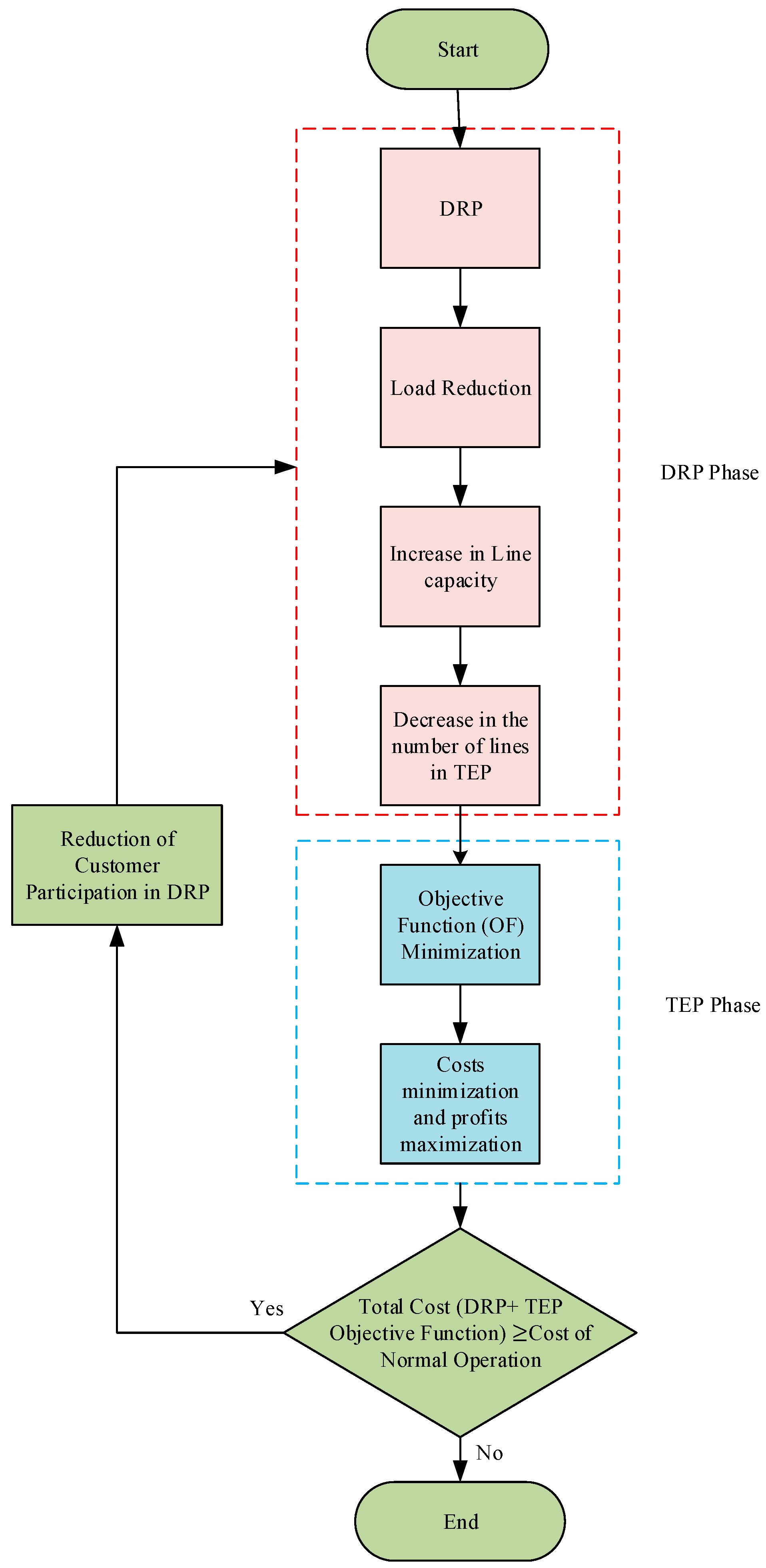
Figure 2.
Flowchart of the TLBO algorithm.
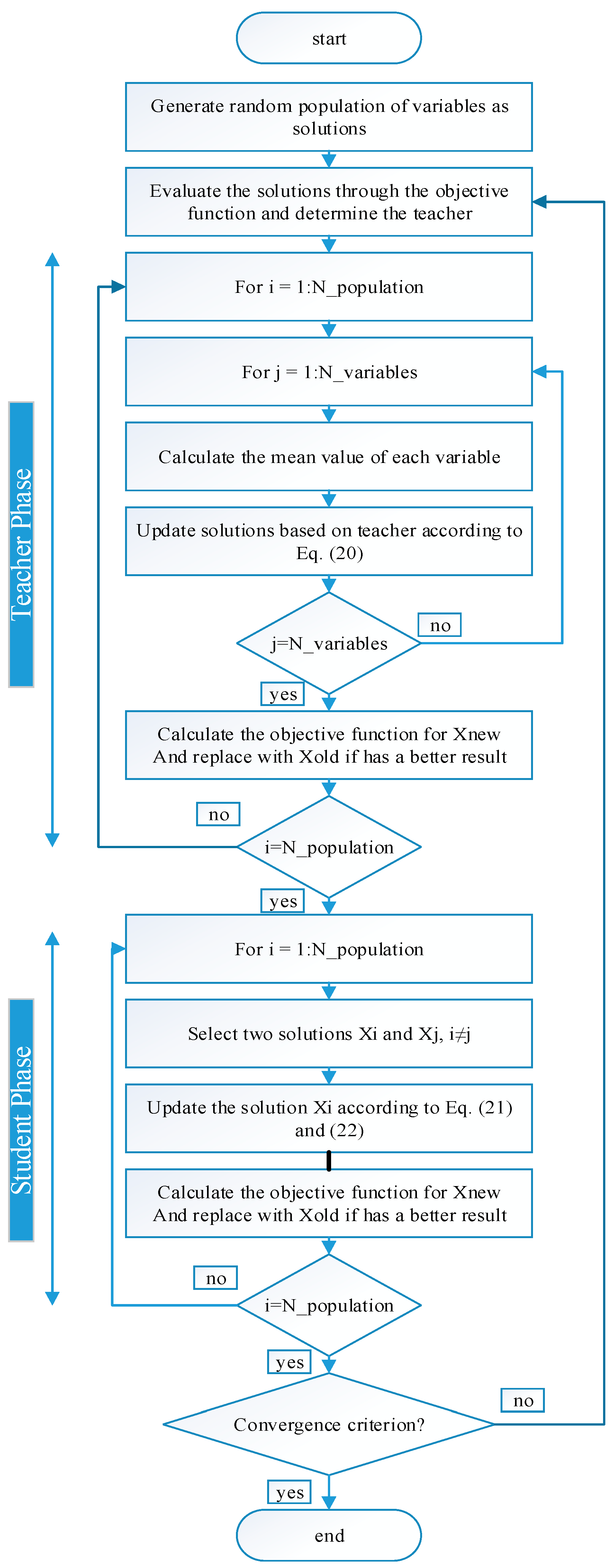
Figure 3.
The six-bus network.
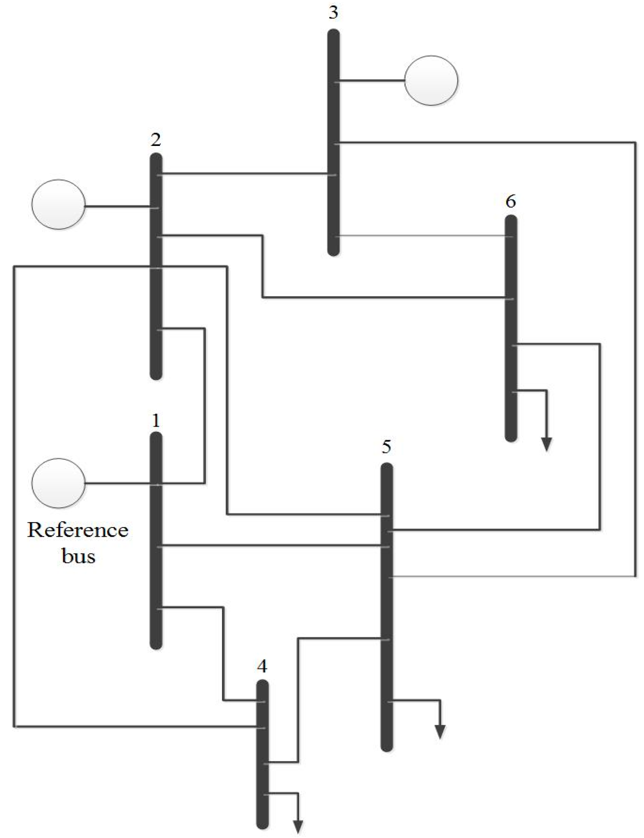
Figure 4.
Load diagram for bus four.

Figure 5.
The bus four load curve before and after the implementation of the demand response program (DRP).
Figure 5.
The bus four load curve before and after the implementation of the demand response program (DRP).

Figure 6.
The bus six load curve before and after the DRP.

Figure 7.
The reduction percentage after DRP implementation.
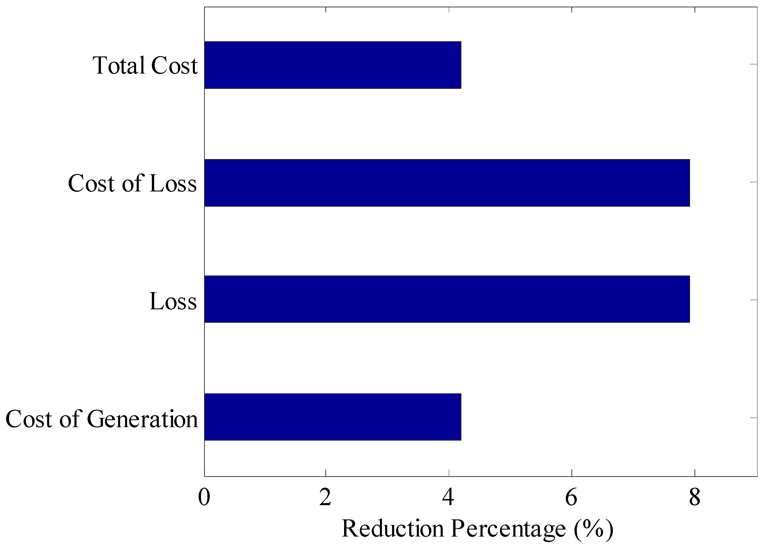
Figure 8.
Costs of different scenarios. Scenario 2: optimal load flow after DRP. Scenario 3: objective function excluding line construction cost. Scenario 4: objective function including line construction cost.
Figure 8.
Costs of different scenarios. Scenario 2: optimal load flow after DRP. Scenario 3: objective function excluding line construction cost. Scenario 4: objective function including line construction cost.


Table 1.
Self- and cross-elasticity.
| Peak | Off-Peak | Valley | |
|---|---|---|---|
| Peak | −0.10 | 0.016 | 0.012 |
| Off-Peak | 0.016 | −0.10 | 0.01 |
| Valley | 0.012 | 0.01 | −0.10 |
Table 2.
The results of Optimal load flow before and after DRP implementation.
| Scenario | Loss (MW) | Cost of Loss ($/h) | Cost of Generation ($/h) | Cost of Line ($/h) | Total Cost ($/h) |
|---|---|---|---|---|---|
| Before DR | 6.908 | 24.04 | 3143.97 | 63.627 | 3231.637 |
| After DR | 6.361 | 22.14 | 3010.87 | 63.627 | 3096.637 |
Table 3.
Results of transmission expansion planning (TEP) for different scenarios in a six-bus network. Scenario 3: objective function excluding line construction costs. Scenario 4: objective function including line construction costs.
Table 3.
Results of transmission expansion planning (TEP) for different scenarios in a six-bus network. Scenario 3: objective function excluding line construction costs. Scenario 4: objective function including line construction costs.
| Scenario | No. of Lines Added Between Two Different Buses | Loss (MW) | Cost of Loss ($/h) | Cost of Generation ($/h) | Cost of Line Construction ($/h) | Cost of DR (S/h) | Total Cost ($/h) |
|---|---|---|---|---|---|---|---|
| 3 | 1–2(3), 1–3(3), 1–4(0), 1–5(3), 1–6(3), 2–3(3), 2–4(0), 2–5(3), 2–6(3), 3–4(3), 3–5(3), 3–6(3), 4–5(3), 4–6(2), 5–6(3) | 1093 | 3.60 | 1868.63 | 108.37 | 670.96 | 2651.56 |
| 4 | 1–2(3), 1–3(0), 1–4(0), 1–5(0), 1–6(0), 2–3(3), 2–4(0), 2–5(0), 2–6(0), 3–4(0), 3–5(0), 3–6(0), 4–5(0), 4–6(0), 5–6(0) | 2.93 | 10.21 | 1868.63 | 68.22 | 670.96 | 2618.02 |
Table 4.
Results of TEP for different scenarios in a -bus network. Scenario 3: objective function excluding line construction costs. Scenario 4: objective function including line construction cost.
Table 4.
Results of TEP for different scenarios in a -bus network. Scenario 3: objective function excluding line construction costs. Scenario 4: objective function including line construction cost.
| Scenario | No. of Lines Added Between Two Different Buses | Loss (MW) | Cost of Loss ($/h) | Cost of Generation ($/h) | Cost of Line Construction ($/h) | Cost of DR (S/h) | Total Cost ($/h) |
|---|---|---|---|---|---|---|---|
| 3 | 1–2(0), 1–3(3), 1–6(3), 1–8(3), 1–9(3), 1–12(3), 1–16(3), 1–17(3), 2–3(3), 2–6(3), 2–8(3), 2–9(3), 2–12(3), 2–16(3), 2–17(3), 3–6(3), 3–8(3), 3–9(3), 3–12(2), 3–16(0), 3–17(0), 6–8(3), 6–9(3), 6–12(3), 6–16(0), 6–17(0), 8–9(3), 8–12(3), 8–16(3), 8–17(3), 9–12(2), 9–16(3), 9–17(0), 12–16(2), 12–17(3), 16–17(0) | 9.79 | 34.09 | 40,309 | 577.14 | 900 | 41,790 |
| 4 | 1–2(0), 1–3(0), 1–6(0), 1–8(3), 1–9(3), 1–12(3), 1–16(3), 1–17(0), 2–3(3), 2–6(0), 2–8(3), 2–9(3), 2–12(3), 2–16(3), 2–17(0), 3–6(0), 3–8(0), 3–9(0), 3–12(0), 3–16(0), 3–17(0), 6–8(3), 6–9(0), 6–12(0), 6–16(0), 6–17(3), 8–9(3), 8–12(3), 8–16(3), 8–17(3), 9–12(0), 9–16(3), 9–17(0), 12–16(3), 12–17(3), 16–17(0) | 10.38 | 36.12 | 40,335 | 536 | 900 | 41,777 |
© 2017 by the authors. Licensee MDPI, Basel, Switzerland. This article is an open access article distributed under the terms and conditions of the Creative Commons Attribution (CC BY) license (http://creativecommons.org/licenses/by/4.0/).
Share and Cite
MDPI and ACS Style
Zakeri, A.S.; Askarian Abyaneh, H. Transmission Expansion Planning Using TLBO Algorithm in the Presence of Demand Response Resources. Energies 2017, 10, 1376. https://doi.org/10.3390/en10091376
AMA Style
Zakeri AS, Askarian Abyaneh H. Transmission Expansion Planning Using TLBO Algorithm in the Presence of Demand Response Resources. Energies. 2017; 10(9):1376. https://doi.org/10.3390/en10091376
Chicago/Turabian StyleZakeri, Amir Sadegh, and Hossein Askarian Abyaneh. 2017. "Transmission Expansion Planning Using TLBO Algorithm in the Presence of Demand Response Resources" Energies 10, no. 9: 1376. https://doi.org/10.3390/en10091376
Note that from the first issue of 2016, this journal uses article numbers instead of page numbers. See further details here.