
Hosting Capacity of the Power Grid for Renewable Electricity Production and New Large Consumption Equipment


Electric Power Engineering, Luleå University of Technology, 931 87 Skellefteå, Sweden
*
Authors to whom correspondence should be addressed.
Energies 2017, 10(9), 1325; https://doi.org/10.3390/en10091325
Submission received: 27 July 2017
/
Revised: 27 August 2017
/
Accepted: 29 August 2017
/
Published: 2 September 2017
(This article belongs to the Special Issue Distribution Power Systems and Power Quality)
Abstract
:After a brief historical introduction to the hosting-capacity approach, the hosting capacity is presented in this paper as a tool for distribution-system planning under uncertainty. This tool is illustrated by evaluating the readiness of two low-voltage networks for increasing amounts of customers with PV panels or with EV chargers. Both undervoltage and overvoltage are considered in the studies presented here. Probability distribution functions are calculated for the worst-case overvoltage and undervoltage as a function of the number of customers with PV or EV chargers. These distributions are used to obtain 90th percentile values that act as a performance index. This index is compared with an overvoltage or undervoltage limit to get the hosting capacity. General aspects of the hosting-capacity calculations (performance indices, limits, and calculation methods) are discussed for a number of other phenomena: overcurrent; fast voltage magnitude variations; voltage unbalance; harmonics and supraharmonics. The need for gathering data and further development of models for existing demand is emphasised in the discussion and conclusions.
1. Introduction
Changes in society are typically initiated and mainly take place outside of the power grid, however, such changes might still affect the electric power grid. Three specific types of changes are currently taking place at the same time, causing a range of serious challenges to the design, planning and operation of the grid:
- i)
- New types of electricity production. There is a shift from large production units connected to the transmission grid to small units connected to the distribution grid, sometimes even connected at low voltage on the customer side of the electricity meter. Driven by the need for a more sustainable energy system, this new production is often of the renewable type and connected through a power-electronics interface. This shift in production, including the expected future developments, is rather well documented in papers, books, and government reports [1,2,3,4].
- ii)
- Changes in electricity consumption. The electricity consumption is where societal changes often have the first impact. There is since many years a general increase in the number of electric devices used. The transition to a sustainable energy system is driving a shift towards more energy-efficient equipment, equipment with a power-electronics interface, and the introduction of new types of equipment. Examples of the latter are electric vehicles [5,6,7] and heat pumps (as a replacement of either gas heating or as a replacement for resistive electric heating) [8]. The replacement of incandescent lamps by compact fluorescent and LED lamps should be mentioned specifically [9]. In developing countries, an increase in wealth is strongly correlated to a growth in electricity consumption.
- iii)
- Changes in the grid. A combination of technical developments on the one hand and societal, environmental and regulatory requirements on the other hand is leading to new types of solutions being used as part of the power grid. The shift from overhead lines to underground cables is one example, but also the slow but on-going introduction of a range of technology that comes under the term “smart grids” [10,11,12]. This new technology is obviously intended to offer better and/or more cost-effective solutions, but unintended consequences of the new technology may still pose a challenge. An overview of some of the unintended consequences for power quality of smart-grid technology is presented in [13].
All these changes create a range of challenges and a lot of research and practical studies have been done and are ongoing to address those changes and the possible challenges. Many studies have been done on the impact of local generation on the distribution grid, where overcurrent and overvoltage are typically the risks being studied [2,14,15,16,17,18]. An overview of the power-quality related challenges for some of the major changes is presented in [19,20]. Some of the specific conclusions from those studies are:
- i)
- The large-scale introduction of active power electronics, in production as well as consumption equipment, results in additional phenomena becoming of importance: interharmonics; DC components and low-frequency subharmonics (“quasi-DC”); and components above 2 kHz (“supraharmonics” [21]).
- ii)
- The amount of capacitance connected to the grid is expected to increase at all voltage levels. This will result in a shift of resonances to lower frequencies. The increased emission at higher frequencies may be (partly) compensated by the shift in resonance to lower frequencies. However, at the same time, the transfer of disturbances will become less predictable.
An international working group [22] recently presented a number of recommendations, key findings and open issues to be addressed because of the integration of solar power. Recommendations were given for a number of power-quality phenomena, including harmonics, supraharmonics, fast voltage variations (faster than 10-min time scale), slow voltage variations (slower than 10 min), overvoltage, flicker, and voltage unbalance. The hosting capacity approach, as was proposed by an international cooperation project in 2004 (see Section 2) is put forward in the report as an important tool for quantifying the impact of solar power on the power system. Additional work is needed, according to the report, for establishing suitable performance indices and corresponding limits.
This paper consists of three main parts. It starts in Section 2 with an overview, partly from a historical insider perspective, of the hosting-capacity approach. This part also includes a discussion on different kinds of uncertainly. A hosting-capacity-based planning approach is presented in Section 3, applied in Section 4.1 through Section 4.6 and discussed in Section 4.7. The description and the application are for overvoltage and undervoltage as these are the phenomena, with the possible exception of overcurrent, for which the best calculation tools, performance indices and limits are available. The third part of the paper contains a detailed discussion about including other phenomena in hosting-capacity studies. For each phenomenon, performance indices, limits and calculation methods are discussed.
2. Hosting Capacity
The term “hosting capacity” was coined in the context of distributed generation by André Even in March 2004 during discussions within the integrated European EU-DEEP project [23,24]. An approach for quantifying the hosting capacity was developed further by others within that same project [25]. The term “hosting capacity” was already in use before 2004, but in rather different context, for example for internet servers [26], for watermarking of images [27] and for the settlement of refugees [28]. Hosting capacity is now widely used as a term and as a methodology by network operators, by energy regulators and by researchers. Many studies have been done where the hosting capacity was calculated, especially for distribution networks and especially for new production, for example [29]. The hosting capacity has also been used to quantify the impact of electric vehicle charging on the grid, for example [30]. The basic hosting-capacity approach was later extended, among others to cover solutions like curtailment [24]. Studies towards estimating hosting capacity are common part of studies by large network operators as part of their strategies towards allowing the integration of more renewable electricity production into their electricity networks [31,32,33].
An important recent development is the introduction of a stochastic approach to hosting capacity [34,35,36,37,38,39]. The stochastic element introduced concerns especially the unknown location of future PV installations in the distribution grid, but it can be extended to include other uncertainties (see Section 2.2).
2.1. Definition and Aim of Hosting Capacity
The hosting-capacity approach, for distributed generation, has been introduced as a transparent communication tool between stakeholders concerning the connection of distributed generation to the grid. The hosting capacity is defined as the amount of new production or consumption that can be connected to the grid without endangering the reliability or voltage quality for other customers [2,25]. Essential to the approach are the selection of performance indices for the grid and acceptability limits for those indices. The hosting capacity is the amount of new production or consumption where the first performance index reaches its limit. This is illustrated in Figure 1 and Figure 2, for two cases involving new production. For example, the risk of overvoltage already increases with very small amounts of new production connected to a part of the grid with only consumption (like in Figure 1); the risk of overcurrent will initially decrease (like in Figure 2). In cases like in Figure 2, it sometimes makes sense to introduce a second hosting capacity value (HC1) at which the performance is the same as for the system without any new generation.
2.2. Uncertainties
When determining the hosting capacity of the grid at a certain location or for a certain part of the grid, several uncertainties play a role. The uncertainty that is most discussed and studied is the variation of wind or solar power production with time. This is somewhat incorrectly referred to as “intermittent” and regularly (but somewhat unwarranted) mentioned as the main concern with integration of renewable electricity production. It is admittedly not possible to predict the solar or wind-power production accurately, more than a few days ahead (for most countries). Even prediction a few hours ahead is often difficult. This limits the usefulness of wind and solar power as a dispatchable source of electricity.
It is however possible, with a reasonable accuracy, to obtain probability distributions for the amount if solar or wind-power production at a certain location, from some basic information about the size of the installation. Weather data, often obtained over several decades with high accuracy, is the basis for the calculation of such distribution functions. Long-term trends are most likely present in the weather, but their impact on the stochastic properties of wind and solar-power production is still expected to be smaller than the impact of other uncertainties.
In a similar way, probability distributions and time series can be obtained for the consumption of individual customers or for groups of customers (from the load of a single distribution transformer, up to the consumption of a whole country). Time series over many years are rare, but the introduction of smart metering makes that data for a few years becomes increasingly available. Consumption patterns are prone to change, and likely faster than weather patterns, but not to the extent that the measurements become useless.
Not all time variations in (renewable-electricity) production and consumption are uncertain. The daily and seasonal variations in solar-power production are very predictable, as an example. When studying solar-power integration for a limited part of the year (e.g., around noon during Summer) the appropriate probability distribution function should be used.
Next to the above-mentioned uncertainties, there exists another level of uncertainty. That kind of uncertainty cannot be obtained from past measurements. Some examples (all related to small-scale solar power), are:
- i)
- Which customers will have a PV installation and how big will these installations be?
- ii)
- Will these installations be three-phase or single-phase connected?
- iii)
- With single-phase connection: to which phase will it be connected?
- iv)
- What will be the direction and tilt of the panels?
- v)
- Will any of the panels follow the sun through single-axis or double-axis mounts?
- vi)
- What type of inverter will the installation have? Will it be one large inverter or a number of smaller inverters?
- vii)
- Will the installation have on-site storage or not? When it has on-site storage, what will its size be, which control algorithms will it use, and will the owner use the storage to participate in day-ahead and balancing markets?
- viii)
- Will the inverter be equipped with voltage and reactive power control?
The answers to all of these questions need to be known before an accurate hosting capacity can be calculated. However, the answers will most likely not be known. Either an educated guess will have to be made or a stochastic approach is needed. The latter is the approach that will be illustrated in Section 4.
2.3. Impacts on the Hosting Capacity
The hosting capacity approach has been developed as a transparent approach aimed at enabling a more open discussion between the different stakeholders. That does however not imply that there is a unique value of the hosting capacity, as resulting from the calculations.
The before-mentioned uncertainties all have their impact on the results of the calculations. In addition, the calculations themselves affect the results. Certain assumptions will have to be made and certain parameter values are needed. The choice of these assumptions and parameter values can have a big impact. Data, especially on the consumption patterns, is not always available when the studies are made and assumptions can have a serious impact. A sensitivity analysis is needed to evaluate if additional data collection and model development are needed. Alternatively, additional stochastic variables can accommodate for the uncertainty.
What has an even bigger potential impact, and where no amount of data collection or model development may help, is the choice of the performance index and the limit (as shown in Figure 1 and Figure 2). These choices depend strongly on the amount of risk that the stakeholders (especially the network operators and their customers) are willing to take. The lower the risk the network operators are willing to take, the lower the hosting capacity.
3. A Hosting-Capacity-Based Planning Approach
A range of hosting-capacity studies are presented in the literature and more are being used in various studies without being published. The hosting-capacity-based planning approach proposed here, consists of the following steps:
- i)
- Estimate the no-load voltage variations in the low-voltage distribution network during those hours of the year that the production from solar power may be high. These are the voltage variations originating from the medium-voltage network.
- ii)
- Estimate the range of the lowest consumption during those hours of the year that the production from solar power may be high.
- iii)
- Estimate the production per installation, during the 10-min period with the highest impact from all installations together. This is not the same as the maximum production per panel, but it can be referred to as an “after diversity maximum production”, next to an “after diversity minimum consumption”.
- iv)
- Add solar power installations in a random way and calculate the distribution of worst-case voltage with increasing amount of solar power.
- v)
- Define a performance index for the network, an appropriate limit for this index, and determine the hosting capacity.
This approach for distribution-system planning can be seen as an adapted version of the classical approach, where an “after diversity maximum consumption” is compared with the capacity of lines, cables and transformers.
The difference between the planning approach used here, and the time-series approach often used in other studies, is that the proposed planning approach immediately considers the worst-case during a longer period, like several years. Distribution-network planning is largely about making sure that the network can cope with for example the highest current through a transformer. It is this worst case that matters. However, also the worst-case value can be treated as a random variable, which is the base for the planning approach presented here. Probability distributions are used, for example for the consumption. These are not the same as the probability distributions obtained from time series. Instead, they are the range of values during those hours of the year that the worst-case situation can occur.
The result of the calculations is thus not the probability distribution of the voltage magnitude, but instead the probability distribution of the worst-case voltage magnitude. Alternatively, one may consider this as the probability distribution obtained over a range of possible futures, all with a different worst-case value. Important advantages of the approach proposed here and applied in Section 4, are:
- i)
- The approach fits closely to existing planning approaches used by distribution companies.
- ii)
- A limited amount of input data is needed.
- iii)
- The results are such that they can be interpreted relatively easy by distribution companies.
- iv)
- Different kinds of uncertainties can be added without changing the basic approach.
- v)
- Any power-system analysis tool can be used to perform the actual calculations.
The limitation of the approach is that it requires certain assumptions, like in step (i) and (ii) above. In practical planning studies, these assumptions might become more based on expert opinions than on actual reproducible studies. Different persons may obtain different results. Such is however common in practical planning studies for distribution grids. With the proposed approach, the assumptions become clearly visible and might trigger further studies.
4. Overvoltage and Undervoltage
4.1. Two Swedish Low-Voltage Networks
To illustrate the calculation of the hosting capacity in a stochastic way for planning purposes, two low-voltage networks in the North of Sweden have been used: a 6-customer rural network; and a 28-customer suburban network. Both networks were used in [39], where the details of the networks can be found. Both networks contain only domestic customers and both networks are three-phase down to the customer. The customer has the possibility of connecting three-phase equipment and of spreading the equipment over the three phases. Note that this is not possible in distribution networks with single-phase laterals, as are common in North America.
4.2. Risks Due to Single-Phase Equipment
In this section (Section 4), the risk of overvoltage and undervoltage due to single-phase equipment will be quantified. Both new production (domestic PV installations) and new consumption (domestic EV chargers) are included in the study. The connection of single-phase equipment is more severe for the grid than the connection of three-phase equipment with the same power rating. Not only is the voltage rise or drop higher for single-phase equipment (three times the current and about twice the impedance), but the other phases are also impacted. Connection of a single-phase EV charger in one phase results in a voltage drop in that phase and a voltage rise in the other phases.
Many hosting capacity studies consider detailed time series of both consumption and production to find at which amount of production voltage or current limits are reached. At higher voltage levels, the data is more likely available than at lower voltage levels. The additional time needed to obtain the data (often several years of data collection are needed) will probably not result in a more accurate result because of remaining uncertainties for example in the details of the installations. This holds especially when the hosting-capacity study concerns the introduction of many devices or installations. In this paper, the authors have therefore chosen for a probability distribution instead of time series. Both methods should be further developed and compared. Some aspects of such comparison are discussed in Section 4.7.3.
4.3. Single-Phase PV in a Rural Network—Overvoltage
The risk of overvoltage due to the introduction of single-phase-connected PV has been studied for the six-customer rural network (see Section 4.1). The probability distribution for the highest voltage is shown in Figure 3 for one through six customers with PV. The following input data has been used for obtaining these distributions:
- i)
- Each installation is connected single-phase and each installation produces 6 kW.
- ii)
- The consumption per customer per phase, during the worst case, is uniformly distributed between 0 and 250 W. This range was obtained from measurements of 10-min values of two customers (one in the rural network and one in the suburban network) and the study of hourly consumption from other customers. The worst case, when considering the risk of overvoltage, is when consumption is low and production is high. High production will likely last a period of one or two hours around noon. The regulation in most European countries sets limits to 10-min values of rms voltage. The lowest 10-min consumption values during one or two-hour periods were considered to obtain the range from 0 to 250 W. Only measurement values around noon during the summer months were used here.
- iii)
- The no-load voltage in the low-voltage network, during the worst case, is uniformly distributed between 238 V and 242 V. The highest 10-min values during one or two-hour periods around noon in the summer months (as obtained from the same measurements) were used to obtain this distribution.
All the random variables in the model are non-correlated. It is further assumed that the PV installations are randomly distributed over the customers and over the phases. The network model used is a simple, linear one, consisting of the node-impedance matrix calculated from the positive and zero-sequence series impedance of the different branches. Positive-sequence and negative-sequence impedances are considered equal. The difference between positive and zero-sequence impedance is considered in the calculations. From the injected and consumed power for each customer and phase, a current vector is calculated. This vector is multiplied with the node-impedance matrix to obtain the vector with phase-to-neutral voltages for all customers and phases. All calculations are performed in Matlab.
A Monte-Carlo simulation is used to generate a large number of combinations of customers and phases with PV. For each combination, the highest phase-to-ground voltage is calculated for each customer terminals. The probability distribution for this voltage is shown in Figure 3. In this case, each distribution was obtained from 10,000 samples.
The plots show how the distribution shifts towards higher voltage magnitudes with increasing amount of solar power. The probability that the overvoltage limit (110% of nominal voltage) is exceeded increases because of this. Already for one customer with PV, there is a small probability that the voltage with one of the customers exceeds the overvoltage limit.
An important advantage of the hosting-capacity approach is its transparency: a well-defined performance index is compared with a well-defined limit. The same should hold when the hosting capacity is used as a planning tool. In this example, the 90th percentile of the distribution shown in Figure 3 has been used as an index and 110% of nominal voltage as a limit. The index value with increasing amount of solar power is shown in Figure 4, where each point is the result of 100,000 simulations. The results are shows for each of the six customers. When one of the 90th percentiles exceeds the 110% limit for one of the customers, the hosting capacity has been exceeded. The hosting capacity is in this case equal to only one customer with PV.
It has been mentioned before (in Section 2.3) that the hosting capacity is not a unique value. Instead, it depends strongly on the model and data used to calculate the index, on the choice of index and on the choice of limit. An example of the latter, with reference to Figure 4, is that the hosting capacity increases to two customers when 112% instead of 110% of nominal is used for the limit.
Figure 5 shows the performance index when it is assumed that each PV installation injects 4 kW instead of 6 kW during the worst case. The resulting hosting capacity is five customers. An example of the impact of the choice of performance index is shown in Figure 6, where the 75th percentile is used instead of the 90th percentile. The production per installation is again assumed 6 kW. The resulting hosting capacity is two customers with PV. In the latter example (Figure 6), it is clear that the increase in hosting capacity goes together with an increase in risk. However, even for the example in Figure 5, the risk of overvoltage increases, as installations may contribute more than 4 kW to the worst case. The choice of model, data, etc. with hosting-capacity calculations is strongly related to the risks that the different stakeholders are willing to take. A brief discussion on this is part of Section 4.7.7.
4.4. Single-Phase PV in a Rural Network—Undervoltage
When considering the risk of undervoltage, other distributions have to be considered for the no-load and no-PV voltages than when considering the risk of overvoltage (Section 4.3). Undervoltage occurs in the phases without PV during periods with high production and at the same time high consumption and low no-load voltages. The high production can occur, like before, around noon during the summer months. Instead of the lowest consumption and the highest no-load voltage, the highest consumption and the lowest no-load voltage should be used as input to the calculation. From the same data as in the previous section, the following input data to the hosting-capacity calculation has been used:
- i)
- Consumption: 1000 W–2500 W per customer per phase. Note again that this is not a typical consumption but an estimation of the amount of consumption that may occur during a worst case for undervoltage due to PV.
- ii)
- No-load voltage: 232 V–236 V.
Like before, 6 kW production per PV installation has been assumed. The resulting probability distributions are shown in Figure 7. Compared to the previous figures, the lowest of the three voltages for each customer has been used as input to the probability distribution function (also known as “cumulative distribution function” or CDF). The results in the figure show that a voltage drop may occur due to solar power, but values less than 95% of nominal during sunny hours are very unlikely. Undervoltage does not set the hosting capacity in this network. However, when the highest consumption occurs during periods with high solar power production, undervoltage may be a bigger concern than overvoltage.
A further look at the results (not presented here), including simulations with 1,000,000 samples, showed that voltages as low as 92% of nominal are actually possible, but with extremely small probabilities: of the order of one per million. This is a good example showing that considering a stochastic approach is the way to go. Such low probabilities do not need to be considered in distribution-system planning.
4.5. Single-Phase PV in a Suburban Network—Overvoltage
The calculations presented in the previous two sections have been repeated for a suburban network with 28 customers (see Section 4.1). The distributions for no-load voltage and consumption are the same as used for the rural network. The results are shown in Figure 8 and Figure 9. The hosting capacity, using the same values as before, equals three customers (see Figure 9).
To illustrate how different parameters affect the outcome of the calculation, a sensitivity analysis has been done. The results of this are shown in Table 1. The hosting capacity turns out to be most sensitive to the percentile used and to the produced power per installation. The percentile used is a matter of how much risk the network operator is willing or even allowed to take in the planning stage. This remains largely an un-explored but very important area. The value of the produced power used in the calculation depends on the size of the individual installations and on the spread in tilt direction and angle between the installations. Some specific studies, with more detailed models including this, are needed for a more accurate estimation of the hosting capacity. See Section 4.7.6.
The hosting capacity turns out to be most sensitive to the percentile used and to the produced power per installation. The percentile used is a matter of how much risk the network operator is willing or even allowed to take in the planning stage. This remains largely an un-explored but very important area. The value of the produced power used in the calculation depends on the size of the individual installations and on the spread in tilt direction and angle between the installations. Some specific studies, with more detailed models including these parameters, are needed for a more accurate estimation of the hosting capacity. See also Section 4.7.6.
4.6. Single-Phase Electric Vehicle Chargers in the Suburban Grid
The same methodology as before has been used to study the risk of undervoltage due to large numbers of single-phase EV chargers. Charging may take place any time of the day and any time of the year. Therefore, lower no-load voltages and higher consumption should be considered than when studying the risk of undervoltage due to PV. The following values have been used for the calculations:
- i)
- Active-power consumption: uniformly distributed between 1500 W and 3000 W.
- ii)
- No-load voltage: uniformly distributed between 230 V and 234 V.
- iii)
- Charging power: 2300 W, 3680 W, 4600 W and 5750 W (corresponding to 10 A, 16 A, 20 A and 25 A).
The resulting performance index is shown in Figure 10 as function of the number of EV chargers that are drawing current at the same time, for 5760 W per charger. The hosting capacity equals nine EV chargers. Assuming 4600 W per charger results in a hosting capacity of 14 chargers (not shown here). For 3680 W and 2300 W per charger, 22 and 28 chargers, respectively can be operating at the same time without the undervoltage limit being exceeded.
4.7. Discussion
The subsections below present some points of discussion, including the need for further work resulting from the presented study. The discussion text refers only to the impact of new production, but a similar discussion is possible for new consumption.
4.7.1. Reactive Power
In this study, only the active power has been included. The reason for this is that the reactive-power consumption of modern domestic customers is small and that the X/R ratio with the supply terminals in a low-voltage network is small. For connection of installations to medium-voltage networks, e.g., solar parks and wind turbines, the reactive power needs to be considered.
4.7.2. Probability Distributions
The study presented here used uniform distributions for the no-load voltage and the consumption during critical hours. More studies, based on measurements as well as on simulations, are needed to find out what are reasonable distributions for these input variables. More advanced stochastic load models exist (for example [40]) and further development and application of those is important. There is, however, a risk of over-sophistication here, where the other uncertainties dominate and make that such advanced models have no higher accuracy than simplified models. With advanced models, there is also the risk that the study loses generality. The development of appropriate load models is an essential part of hosting-capacity studies, next to the development of appropriate models for new production and consumption.
In the study, it was assumed that the no-load voltage was independent on the amount of customers with PV. It requires further study to find out to which extent this no-load voltage is affected by solar power elsewhere in the same medium-voltage network. Some positive correlation can be expected here: when the number of customers with PV increases in a low-voltage network, it is also likely to increase in neighbouring low-voltage networks supplied from the same medium-voltage feeder.
4.7.3. Time Series
The study presented here used probability distribution functions together with a fixed value of the solar-power production. An alternative, commonly used in other studies, is to use time series for both production and consumption. A discussion is needed on the advantages and disadvantages of these two methods. In that discussion, the main comparison should be between time series based on measurements and probability distributions or time series obtained from stochastic models. With the former approach, all the time series should be obtained over the same or an equivalent measurement period. The time series should be sufficiently long to cover all combinations (maximum and minimum production, maximum and minimum consumption, but even medium values that could combine towards a worst case). This requires data collection over several years, to include year-to-year variations.
The main advantage of using measured time series is that these are closest to reality and therefore include all phenomena and correlations as they occur in reality. An example is the relation between solar power production and electric heating or cooling [41].
Comparison studies are needed, between measured time series, probability distributions, and time series obtained from more advanced stochastic models. Differences between the results from the different approaches do however not always imply that one method would be superior compared to another.
The approach presented here can be combined with the use of (measured or generated) time series. Instead of taking one value for consumption and no-load voltage for each spread of the PV panels over the customers and phases, time series are used for each of such spreads. This will bypass the discussion on when the production is expected to be highest (Section 4.7.6), but it will require much more data and calculations.
The voltage-quality regulations in many countries set limits to the 95th percentile of the rms voltage calculated over a 10-min window. This value shall not exceed the overvoltage limit, typically at 110% of nominal voltage. During the planning, the distribution company may still decide to use the highest voltage as a criterion. Alternatively, the 95th percentiles can be used for planning. The plots in Figure 3 and similar would in that case have to show the distribution of the 95th percentile of the voltage for random customers and phases with PV. The use of time series would be a possible choice; but not necessarily, time series for the whole year would be needed. Those time series can be limited to periods with high or low production and/or consumption; for example around noon during summer. Alternatively, the estimated values (i, ii and iii) in Section 3 can be adjusted (see Section 4.7.2).
4.7.4. Need for Data Collection
Much of the work towards further developing the hosting-capacity approach requires measurement data. The use of measured time series obviously requires large amounts of data. The choice of probability distribution for the consumption and the development of more advanced load models is also not possible without significant amounts of data available.
Such data might be available to the network operator, for example in the form of hourly metering. However, the data is in most cases not available to universities or research institutes that work on model development. There is no direct solution to this dilemma as this involves consumption patterns from individual domestic customers with important privacy implications.
Data collection on consumption and consumption patterns for many domestic customers should however still be pursuit. One way or the other, such data should become available for research and education. The set of test feeders, some with load data, collected by [42] is an appropriate platform for making such data available.
4.7.5. Generality of the Results and of the Method
The results of the study presented here are not valid beyond the specific two networks studied, and even for those only under the assumptions presented. The example’s only aim is to illustrate the method. Network operators should use data from their own networks to estimate the hosting capacity as part of their distribution-system planning.
The calculations used here were performed using Matlab only, but any other power-system analysis package can be used for this. In fact, several network operators are developing tools using such packages to estimate the hosting capacity and to create hosting-capacity maps.
Although the specific results are only valid for the studied networks, the method itself has a broader applicability. The method should be applied to different low and medium-voltage networks, to find out how general the results are, but also to evaluate the broader applicability of the method.
The two example networks used here are typical Swedish low-voltage networks, dimensioned to accommodate electric heating. This will result in a higher hosting capacity than for grids only dimensioned for non-electric domestic consumption. The approach should be applied to networks in countries without electric heating, like in the more southern parts of Europe. Both networks, like all Swedish distribution grids, are three phase all the way down to the domestic customer. Two-phase and three-phase equipment is common with domestic customers in Sweden. The approach should be applied to networks dominated by single-phase laterals, like in North America.
The consumption of domestic customers in Sweden is rather constant, with mainly a small downward trend due to increased energy efficiency. This allows the use of a “background consumption” based on measurements with the new production or consumption added to this. This approach is not possible for grids in developing countries where load growth could be significant.
4.7.6. Production per Installation during the Worst Case
In the study presented here, a fixed production per PV installation during the worst-case was used. It was shown from a sensitivity analysis (Table 1) that this value has a big impact on the obtained value for the hosting capacity.
Studies are needed to determine how to get a good model for the production per installation during those hours of the year that the highest production can be expected. One of the questions that has to be answered is, “what are the hours of the year during which the production from solar may be high?” The answer to this question depends for example on the spread of roof top directions. When all rooftops face south, the panels will produce the same amount and the period of peak production will be relatively short. When there is a spread in rooftop direction, the period of expected peak production will be longer but the peak will be smaller. Both measurements and simulations are needed to answer this question.
Instead of a fixed value for the production during the worst case, a stochastic model could also be considered here. The stochastic element is again not in the variation of production with time, but in the uncertainty of the contribution of an individual panel to the worst-case situation.
4.7.7. Choice of Performance Indices and Limits
An essential discussion in hosting capacity studies concerns the choice of performance indices. This discussion started soon after the introduction of the term for the integration of distributed generation. A subject heavily discussed initially was the choice of the appropriate index to quantify the performance of the supply, for example the highest 10-min rms voltage or the 95th percentile of the 3-s rms voltages. This is largely a regulatory issue. More recently, and during the study presented here, the discussion is moving towards the choice of indices for planning under uncertainty. The sensitivity study (Table 1) showed that the percentile value has a big impact on the obtained hosting capacity.
The choice of percentile value is strongly related to the amount of risk carried by the different stakeholders. Important input to the choice of percentile values is who carries this risk and what the possible consequences are. The smaller the consequences, the higher the risk that can be taken.
The selection of the percentile values (and risk management in general) is not a sole power-engineering issue, but it is still very important. This is where economics, social aspects, legal and regulatory aspects, politics and even psychological aspects have to be included in the studies. A new line of interdisciplinary research is needed to address this.
5. Other Phenomena
Section 4 illustrates several aspects of the hosting-capacity approach, through overvoltage and undervoltage. These are however not the only phenomena that can set the hosting capacity (i.e., can set limits to the amount of new production or new consumption that can be connected). Several other phenomena are discussed in the forthcoming sections. As of yet, there is no complete list of phenomena and indices for hosting-capacity studies. An attempt at creating such a list is presented in [43]. With reference to Figure 1 and Figure 2, calculating the hosting capacity requires the following tools and information:
- i)
- A generally accepted performance index.
- ii)
- A limit for the performance index that forms a border between “acceptable performance” and “unacceptable performance”.
- iii)
- A method for calculating the value of this index, either deterministically or in a stochastic way, as a function of the amount of new production or consumption.
These three requirements will be used in the forthcoming sections to discuss the hosting-capacity approach for different phenomena. In those sections, like in Section 4, the aim is to strike a balance between the need for accuracy on one hand and the availability of data and models on the other hand.
5.1. Overcurrent
5.1.1. Performance Indices
Excessive currents (overcurrent) lead to excessive heating with too high temperatures as a result. As this is a thermal issue, the rms current is the obvious choice as base for performance indices. As voltage variations are normally small, the apparent power can be used instead. If reactive power is small, active power can be used instead of apparent power.
Methods for calculating currents through the grid are very similar to methods for calculating voltages. In fact, a load-flow calculation will result in both voltages and currents. When considering them in hosting-capacity studies, some differences need to be considered. The first difference concerns the importance of the phenomenon for the performance of the grid. In [2] and [44], a distinction is made between primary and secondary aims of the power system. In the same way, a distinction can be made between “primary performance indices” and “secondary performance indices” for the hosting-capacity approach. Voltage magnitude would be a primary performance index: something that matters directly to the network users. The current through for example a transformer is however not of direct concern for the network users; it is a secondary performance index. The overloading of a component will quickly result in an interruption for all network users downstream of the overloaded component (either because that component fails or because the protection removes the component to avoid its failure). Avoiding overloading is thus also in the interest of the network user. The probability of an interruption due to transformer overloading would be a primary performance index.
The second difference is in the limit values to be used in the hosting capacity studies. The actual values for current can be obtained in similar ways as before, through “after diversity maximum production”, “after diversity minimum consumption”, etc. The challenge lies in the choice of maximum-permitted-value of, for example, the current through the transformer. For voltage-magnitude variations, the 10-min rms value is defined in standards and regulation, so that the choice becomes easy.
The window over which the value should be calculated depends on the thermal time constant of the cable, line or transformer under study. Information on this can be obtained, for example, from the increasing volume of works on dynamic rating [45]. Here it should be considered that much of the work on thermal time constants is directed towards short circuits where adiabatic temperature rise can be considered. For the lesser overloads that are part of hosting capacity studies, this assumption would likely lead to an underestimation of the hosting capacity. From the literature [46,47,48], time constants between minutes and hours were found. A 10-min value would be a good compromise, given the above range of thermal time constants. Nevertheless, when only 1-hour values are available (e.g., from hourly metering) those also seem to be reasonable.
5.1.2. Limits
In case apparent power or active power is used for the performance index, a margin is appropriate to compensate for the incompleteness in the model. For example, a 10% reduction in limit could be used to compensate for the possible 10% reduction in voltage when apparent power is used instead of rms current. This reduction in limit corresponds mathematically to the assumption that voltage, active power and reactive power are stochastically independent. A more complete model, supported by more complete measurement data, will typically result in an increase in hosting capacity, as was illustrated for a simple case in [49]. With many hosting capacity studies, the more data is available, the less safety margins are needed, and the higher the hosting capacity.
5.1.3. Calculation Methods
The calculation of the currents through a cable, line or transformer, with increasing levels of new production or consumption, is straightforward. The new current is added, in the complex plane, to the existing current. Stochastic methods can be used in the same way as before: a fixed limit for the maximum-permissible current has to be decided, corresponding to the 110% and 90% limits used for the studies in Section 4. An example of such a study is given in Section 5.1.4. Alternatively, a detailed thermal model of the line, cable or transformer can be used together with time series of production and consumption. Many studies use such time series and compare the resulting currents with a maximum current value, e.g., [50].
5.1.4. Planning Example
To illustrate the use of the hosting-capacity approach in distribution, assessing the risk of transformer overload, a similar example as in Section 4 is presented here. This example concerns a 500-kVA transformer supplying 83 customers. When all customers would have a single-phase-connected PV installation (6 kW injected power), they would all together produce 500 kW. When equally distributed over the three phases, this would exactly correspond to the transformer rating. Note that reactive power has not been considered here, partly to simplify the calculations, but also because its impact is limited and because reactive-power consumption from domestic customers is small. For an actual planning study, it is recommended to consider the reactive power and even its possible changes in the future. The results are shown in Figure 11 and Figure 12. Figure 11 gives the probability distribution of the highest single-phase current through the transformer. The consumption per phase has again been assumed uniformly distributed between 0 and 250 W. The current increases when more customers install solar power. However, even when 40 (out of 83) customers have solar power, single-phase connected, the probability that the transformer will be overloaded is still very small.
For the application of the hosting-capacity approach, it is again necessary to define a performance index and a corresponding limit. For this example, four different percentile values (50th, 75th, 90th and 95th) have been used as indices, with the (single-phase) transformer rating as a limit. The result is shown in Figure 12. For up to about five customers with PV, the current index is not affected. For low amounts of PV, the highest transformer loading occurs for maximum load and not for maximum production. Here it is important to realize that “maximum load” corresponds to the period of the day and year when highest solar production can be expected. This is not in any way related to the highest annual consumption.
From Figure 12, the hosting capacity is shown to depend on the percentile value, i.e., on the amount of risk that the network operator is willing and allowed to take. The hosting capacity ranges from 63 (when using the 95th percentile) up to 76 (50th percentile). The impact of the percentile value on the hosting capacity is less than for overvoltage (Table 1).
5.2. Fast Voltage Magnitude Variations
Fast voltage magnitude variations occur because of fast variations in production or consumption.
5.2.1. Performance Indices
Standard indices exist for the fastest voltage magnitude variations; at time scales less than one minute. The short-term and long-term flicker severity (Pst and Plt, respectively) are defined in IEC 61000-4-15; IEC 61000-4-30 gives a definition of (individual) rapid voltage changes. Both definitions are however strictly measurement based, which especially for flicker severity requires detailed models.
Incandescent lamps, which have been the base for the flicker-severity indices, are replaced by other types of lamps in most countries. The flicker-severity indices can no longer be considered as primary performance indices. Their future role as secondary performance indices (of importance to the network operator but not of direct importance to the network user) remains unclear.
For the time scale between 1 s and 10 min (the lower limit for standards on slow voltage magnitude variations in most countries) no standardized or generally accepted indices exist. An index referred to as “very-short variations”, was proposed in 2005 [51,52], but received only limited following [53,54,55,56,57,58,59]. However, the need for performance indices in this range of time scale remains big: this is where the main impact of fast variations in production with solar-power installations will be, as was quantified among others by [60].
5.2.2. Limits
Limits exist for flicker severity and for the number of rapid voltage changes. No limits exist for voltage magnitude variations in the time scale between 1 s and 10 min.
5.2.3. Calculation Methods
Three different phenomena were mentioned in Section 5.2.1, all of which require different methods for calculation. Flicker severity requires either time series with very high time resolution (for example 20 ms) or the use of simplified aggregation rules for example as proposed in IEC/TR 61000-3-7.
For rapid voltage changes, simple voltage calculations (using only the source impedance at the point of connection or at point of common coupling) are sufficient to obtain the step in voltage due to a step in current. The latter can be the start of charging of an electric vehicle but also the unnecessary tripping of a PV installation due to its anti-islanding protection.
5.3. Voltage Unbalance
Voltage unbalance occurs due to the connection of large single-phase devices; both single-phase-connected PV and electric car chargers fall in this category.
5.3.1. Performance Indices
The ratio between negative-sequence and positive-sequence voltage is used as performance index in both IEC and IEEE standards. As the magnitude of the positive-sequence voltage shows limited variation, the negative-sequence voltage can also be used as an index. Next to that, IEEE and NEMA define some additional indices including the difference between highest and lowest line voltage. The different IEC, IEEE and NEMA definitions, all referred to as “unbalance”, are compared in [61,62,63] where it for example is shown that different definitions can give rather different values for the unbalance.
The negative-sequence voltage is a useful index to quantify the impact of unbalance on three-phase rotating machines directly connected to the grid. The impact of unbalance on such devices is a thermal issue, so that 10-min values are appropriate.
For machines connected through a three-phase rectifier, like adjustable-speed drives, and for other equipment connected through a three-phase converter, the difference between the line voltages is a better index. This difference results in current unbalance for three-phase converters that in turn can result in unwanted tripping of the converter [64]. As shown in [62] this value is 87% to 101% of the absolute value of negative-sequence voltage, depending of the phase angle of the latter. As this is a protection issue, a value over a much shorter time scale is needed, like a one-second or three-second value.
5.3.2. Limits
For the negative-sequence unbalance (the IEC definition), a limit of 2% holds for low-voltage networks in many countries. See [65] for an overview of regulatory limits in European countries. Strictly speaking, the indictor is defined as the ratio between negative and positive-sequence voltage. When the calculations give the negative-sequence voltage (or when nominal positive-sequence voltage is assumed) a correction might have to be made for the limit. Assuming that the positive-sequence voltage can be as low as 90% of nominal, and assuming that negative and positive-sequence voltage are stochastically independent, the limit has to be reduced from 2% to 1.8%. There are no limits based on the IEEE and NEMA definitions of unbalance. When 3-s values are used instead of 10-min values, a higher limit than the IEC limit of 2% seems appropriate.
5.3.3. Calculation Methods
The negative-sequence transfer impedance matrix is used in [39] to calculate the increase in negative-sequence voltage in a low-voltage network with increasing number of single-phase-connected PV installations. The negative-sequence impedance of lines, cables and transformers is equal to their positive-sequence value. That can also be generally assumed for the source impedance of public medium-voltage networks. For industrial medium-voltage networks, large rotating machines might result in a lower value for the negative-sequence than for the positive-sequence source impedance.
The presence of three-phase equipment in the low-voltage network may have to be considered as well in the transfer-impedance matrix. The presence of three-phase equipment, like variable-speed heat pumps (common in Sweden), results in a reduction of the negative-sequence transfer impedance and thus in an increase of the hosting capacity. For a planning study, a value or range of values has to be estimated for three-phase equipment that is connected during hours with high amount of production from solar power. In [39] it was assumed that this could be a very small amount, so that its impact on negative-sequence impedance could be neglected. This assumption may result in an underestimation of the hosting capacity.
In [39] the same networks were used as in Section 4. That allows a comparison of the results. The hosting capacity for unbalance, assuming a 1.5% limit for the negative-sequence voltage and the 90th percentile as performance index, was estimated as 3 customers for the 6-customer network and 26 customers for the 28-customer network. The results from the overvoltage studies were: two customers for the 6-customer network (from Figure 4) and up to 22 customers for the 28-customer network (from Table 1).
Important for a complete picture of the hosting capacity is to consider the background voltage unbalance, i.e., the voltage unbalance without connection of any new production or consumption. Here it is important to consider that negative-sequence voltage is a complex quantity, consisting of magnitude and phase angle. During power-quality measurements, the phase angle of the negative-sequence voltage is normally not recorded. This is partly because there is no measurement definition of this angle available.
When the NEMA/IEEE definition of unbalance is used, the negative-sequence transfer impedance is not sufficient for the calculations. Either the complex phase voltages should be used; or separate impedances for positive, negative and zero-sequence components. The latter allows the incorporation of the impact of three-phase-connected equipment on the unbalance. In addition, information on background unbalance may be hard to obtain and require dedicated measurement campaigns.
5.4. Harmonic Voltage Distortion
Harmonic voltage distortion occurs because the current injected by the device is not sinusoidal. The bigger the device, the bigger the impact is of even a small amount of waveform distortion. Even when the relative emission (in percent of rated current) is small, the total impact on the grid can still be significant. With the connection of multiple devices, both the transfer impedance and aggregation rules should be considered.
5.4.1. Performance Indices
Standard indices are defined for each of the individual harmonics and interharmonics, and for total harmonic distortion in IEEE 519, IEC 61000-4-7 and IEC 61000-4-30. Normally, only 10-min values are considered as the impact of harmonics is considered a thermal phenomenon. However, for power-electronic converters and for certain types of protection of other equipment, unwanted protection operation can result from high harmonic or interharmonic distortion. Values obtained over shorter periods, like 1 or 3 seconds, should be used to study such impacts.
In IEC 61000-4-7, both groups and subgroups are defined for harmonics up to order 40 (i.e., 2 kHz in a 50 Hz system) and interharmonics. However, in IEC 61000-4-30 it is stated that the harmonic and interharmonic subgroups should be used when quantifying power quality. Therefore, those are also most appropriate for hosting-capacity studies.
5.4.2. Limits
The selection of limits for use in hosting-capacity studies is not obvious, despite the presence of a range of limits (“objective values”) in national and international standards. Voltage characteristics are given in EN 50160; compatibility levels in IEC 61000-2-2; planning levels can be selected by each network operator themselves, but most of them follow the indicative planning levels from IEC/TR 61000-3-6. Especially the latter deviate a lot from the other ones and it is not obvious which limits should be used.
One approach is to consider a hosting-capacity study as a planning study, in which the planning levels would be appropriate. However, in more and more countries are the planning levels replaced by the limits set in local regulations. These are in turn, at least in Europe, strongly based on the voltage characteristics in EN 50160.
The final decision on the choice of limits, as many other choices in a hosting-capacity study, is part of the risk management between the different stakeholders. A complete hosting capacity study should therefore also consider a mapping of the risks as carried by the different stakeholders. Such a mapping is beyond the scope of this paper.
5.4.3. Calculation Methods
The choice of performance indices and limits is relatively straightforward for harmonics. However, the main barrier is the lack of appropriate calculation models, especially when considering low-voltage and medium-voltage networks.
The basic approach used in the literature is the source impedance or the transfer impedance matrix [66,67,68,69,70]; for harmonic frequencies instead of for the negative-sequence voltage as in the case of unbalance [39] or the equivalent impedances for single-phase loads as in the case of overvoltage due to single-phase PV. Once the injected harmonic currents and the impedance values are known, the harmonic voltage distortion can be calculated as a function of the amount of new production or consumption. Obtaining those values is however not easy and with the current state of the art no generally accepted method is available. This was illustrated by several studies on the impact of compact fluorescent lamps and LED lamps on the waveform distortion. Simulation studies concluded that the voltage and current distortion would increase [71,72]; measurements showed however that this was not the case and that the distortion was simply not impacted [73,74,75,76]. Acceptable harmonic models exist for the components of the power system (cables, lines and transformers) but several barriers remain before a complete model is available for use in hosting-capacity studies:
- i)
- The emitted harmonic current is impacted by the voltage distortion at the terminals of the equipment. This phenomenon has been observed early for diode rectifiers like the ones used in televisions [77] and was explained and quantified by a model in [78]. That impact was shown to be limited and the emission for a clean supply voltage was in most cases the worst case and the one reasonably useable for harmonic studies. With modern power-electronic equipment, with an actively controlled interface, there are observations showing the contrary, the emission for a distorted supply voltage can be much higher than for a sinusoidal supply [79,80,81,82].
- ii)
- iii)
- The connecting of new production or consumption will change the impedance of the low-voltage customer and therewith the harmonic transfer impedance. There exist no acceptable models for new devices like PV inverters or EV chargers. Some measurements are presented in [86,87,88,89] but there are big variations between manufacturers and for future equipment guesses have to be made.
- iv)
- The statistical aggregation between different sources of harmonics is not known. This holds for the aggregation between different new devices (e.g., between different PV inverters) but also for the aggregation between the new devices and the background distortion. The aggregation between individual wind turbines has been studied by some authors [90,91,92] but it is not known if similar conclusions hold for PV inverters, EV chargers or other large low-voltage equipment like heat pumps [22,71,93].
5.5. Supraharmonics
Supraharmonics (waveform distortion in the frequency range between 2 kHz and 150 kHz) are injected by an increasing amount of devices connected to the grid. Supraharmonics are mainly due to active switching in the grid-interface of the devices. The transfer and aggregation of supraharmonics is significantly different from the transfer and aggregation of harmonics. To do a complete hosting capacity study of supraharmonics is to date not feasible, simply because there are no established limits or indices for distortion in this frequency range. This section will instead give a general description of supraharmonics, what levels can be expected and how they are transferred through the grid.
Supraharmonics commonly originate from two sources: power-electronic converters and transmitters of power line communication [21], the former being the focus here. Magnitude, frequency and duration of the emission vary between different devices but come in three general types: constant in magnitude and/or frequency over one cycle of the power system frequency; varying in magnitude and/or frequency over one cycle of the power system frequency or having a transient character [94]. For household devices the emission is in most cases of the varying type, two examples can be seen in Figure 13, where the Short Time Fourier Transform of a fluorescent lamp and a heat pump is shown. The emission from the fluorescent lamp varies in frequency and in magnitude during 20 ms whereas the emission from the heat pump varies only in amplitude as it appears and disappears four times per cycle.
In most cases, supraharmonics do not propagate over long distances. Damping in cables is one of the causes of this. More importantly, other devices connected to the low voltage network offer a low impedance path for these currents so that they tend to flow mainly between devices [95,96]. However, it is still feasible that supraharmonics can transfer through the grid. In [97] it is shown, through both measurements and simulations, that a resonance between the distribution transformer and an 800 m long cable amplified a 35 kHz voltage component on the low-voltage side of the transformer five times. To predict how the emission from an installation or device will transfer through the grid is difficult because of the dominating impact from connected. To correctly predict what is connected at a certain grid at any given moment in time would not be possible.
Many modern household devices emit supraharmonics to some extent. In [94] it is concluded that more than half of the household devices on the market have identifiable supraharmonic emission. There is a large diversity in magnitude and frequency between different devices, even if they are of the same type. For instance, measurements of about 80% of the types of EV chargers on the German market show that the switching frequency is between 9 and 100 kHz with a magnitude between 8 mA and 1.8 A [98].
The emission from a PV inverter and a heat pump are shown in Figure 14. The dominating emission is seen at 16 kHz from the inverter and at 18 kHz from the heat pump (note that these are just two examples, other PV inverters and heat pumps on the market will typically show a completely different behavior). For the measurements seen on the left in Figure 14, the devices are connected alone at the test site. For the measurements seen on the right, other devices are connected nearby; a TV close to the PV inverter and an induction stove close by the heat pump. When other devices are connected to the same phase, the emission at 16 kHz and 18 kHz originating from the inverter and the heat pump is increased, two and five times respectively. This indicates a resonant frequency close to 16 kHz or 18 kHz. The impact of neighbouring equipment on the emission level of supraharmonics from an EV charger is discussed in detail in [99].
6. Conclusions
The concept of hosting capacity has been introduced as a transparent tool allowing an open discussion between different stakeholders with the integration of distributed generation. This transparency remains an important characteristic of the hosting-capacity approach also when it is used as a planning tool for both new production and new consumption, as illustrated in this paper. Any hosting-capacity study requires (directly or indirectly) three parts: a performance index; a corresponding limit; and a method to calculate the value of the performance index as a function of the amount of new production or consumption. Further work is needed towards almost all of these before complete hosting-capacity studies can be done.
A hosting-capacity-based planning approach has been presented in this paper. The approach requires a network model, limited input data and a Monte-Carlo simulation to address the uncertainties. The approach has been applied to overvoltage and undervoltage due to increasing amounts of solar power and electric-vehicle chargers in low-voltage networks. A sensitivity analysis shows that the size of the PV inverters and the performance index have the main impact on the hosting capacity.
It is shown that, with single-phase connection of PV, not only overvoltage but also undervoltage limits may be exceeded. The hosting-capacity values obtained from the case studies cannot be generalized and applied to other low-voltage networks.
For the main impacts of new production and consumption, overvoltage, undervoltage and overcurrent, the calculation tools are available. However, suitable models to describe the existing situation in terms of voltage and current are missing. Different approaches are discussed in the paper, but as of yet no method is the dominating one. Data gathering is an important step in the development of such models.
For harmonics and interharmonics, acceptable calculation models remain missing and further work is needed towards those. Measurements are needed to develop component models so that harmonics and supraharmonics can be sufficiently accurately predicted for future grids. Generally, further work is needed towards selecting appropriate performance indices and the corresponding limits. This requires an interdisciplinary research effort.
Acknowledgments
This studies presented in Section 3 of this paper have been funded by a number of Swedish network operators through the smart-grid program of Energiforsk, by Skellefteå Kraft and by Umeå Energi. Some of the simulations shown in Section 3 were performed by Cecilia Karlsson as part of her final-year project. The measurements referred to in Section 3 were performed by Anders Larsson, Martin Lundmark and Mikael Byström.
Author Contributions
Both authors contributed to this publication; Math H. J. Bollen has been involved in the hosting-capacity approach since the term was first coined in 2004; Sarah K. Rönnberg has been a contributor to introductory parts of the paper; a discussion partner for the simulations presented in Section 3 and the main author for Section 5.4 and Section 5.5.
Conflicts of Interest
The authors declare no conflict of interest.
References
- Tagare, D.M. Electricity Power Generation: The Changing Dimensions; Wiley: Hoboken, NJ, USA, 2011. [Google Scholar]
- Bollen, M.; Hassan, F. Integration of Distributed Generation in the Power System; Wiley-IEEE Press: Hoboken, NJ, USA, 2011. [Google Scholar]
- Staffell, I.; Brett, D.J.L.; Brandon, N.P.; Hawkes, A.D. Domestic Microgeneration: Renewable and Distributed Energy Technologies, Policies and Economics; Routledge: Abingdon, UK, 2015. [Google Scholar]
- International Energy Agency. Medium-Term Renewable Energy Market Report 2016—Market Analysis and Forecasts to 2021; International Energy Agency: Paris, France, 2016.
- International Energy Agency. Global EV Outlook 2016—Beyond One Million Electric Cars; International Energy Agency: Paris, France, 2016.
- Matulka, R. The History of the Electric Car; Department of Energy: Washington, D.C., USA, 2014.
- Wu, Q. Grid Integration of Electric Vehicles in Open Electricity Markets; Wiley: Hoboken, NJ, USA, 2013. [Google Scholar]
- Chua, K.J.; Chou, S.K.; Yang, W.M. Advances in heat pump systems: A review. Appl. Energy 2010, 87, 13611–13624. [Google Scholar] [CrossRef]
- Waide, P. Phase out of Incandescent Lamps—Implications for International Supply and Demand for Regulatory Compliant Lamps; International Energy Agency: Paris, France, 2010.
- Bollen, M. The Smart Grid—Adapting the Power System to New Challenges; Morgan & Claypool: San Rafael, CA, USA, 2011. [Google Scholar]
- Hatziargyriou, N. Microgrids: Architectures and Control; Wiley-IEEE Press: Hoboken, NJ, USA, 2014. [Google Scholar]
- Liu, C.-C.; McArthur, S.; Lee, S.-J. Smart Grid Handbook; Wiley: Hoboken, NJ, USA, 2016. [Google Scholar]
- Bollen, M.H.J.; Das, R.; Djokic, S.; Ciufo, P.; Meyer, J.; Rönnberg, S.K.; Zavoda, F. Power quality concerns in implementing smart distribution-grid applications. IEEE Trans. Smart Grid 2017, 8, 391–399. [Google Scholar] [CrossRef]
- Dugan, R.C.; McGranaghan, M.F.; Santoso, S.; Beaty, H.W. Electric Power Systems Quality; McGraw-Hill: New York, NY, USA, 2012. [Google Scholar]
- Jenkins, N.; Allan, R.; Crossley, P.; Kirschen, D.; Strbac, G. Embedded Generation; Institution of Engineering and Technology: Stevenage, UK, 2000. [Google Scholar]
- Lopes, J.A.P.; Hatziargyriou, N.; Mutale, J.; Djapic, P.; Jenkins, N. Integrating distributed generation into electric power systems: A review of drivers, challenges and opportunities. Electr. Power Syst. Res. 2007, 77, 1189–1203. [Google Scholar] [CrossRef]
- Freris, L.; Infield, D. Renewable Energy in Power Systems; Wiley: Hoboken, NJ, USA, 2008. [Google Scholar]
- Masters, C.L. Voltage rise: The big issue when connecting embedded generation to long 11 kV overhead lines. IET Power Eng. J. 2002, 16, 5–12. [Google Scholar] [CrossRef]
- Rönnberg, S.K.; Bollen, M.H.J. Power quality issues in the future electric power system. Electr. J. 2016, 29, 49–61. [Google Scholar] [CrossRef]
- Rönnberg, S.K.; Bollen, M.H.J.; Langella, R.; Zavoda, F.; Hasler, J.-P.; Ciufo, P.; Cuk, V.; Meyer, J. The expected impact of four major changes in the grid on the power quality—A review. CIGRE Sci. Eng. 2017, 8, 5. [Google Scholar]
- Rönnberg, S.K.; Bollen, M.H.J.; Amaris, H.; Chang, G.W.; Gu, I.Y.H.; Kocewiak, Ł.H.; Meyer, J.; Olofsson, M.; Ribeiro, P.F.; Desmet, J. On waveform distortion in the frequency range of 2 kHz–150 kHz—Review and research challenges. Electr. Power Syst. Res. 2017, 150, 1–10. [Google Scholar] [CrossRef]
- CIGRE JWG C4/C4.29, Power Quality Aspects of Solar Power, CIGRE Technical Brochure 672. 2016. Available online: www.e-cigre.org (accessed on 24 July 2017).
- Bourgain, G. Integrating Distributed Energy Resources in Today’s Electrical Energy System; Book Presenting the Results of the EU-DEEP Project; ExpandDER: Saint Denis le Plaine, France, 2009. [Google Scholar]
- Etherden, N. Increasing the Hosting Capacity of Distributed Energy Resources Using Storage and Communication. Ph.D. Thesis, Luleå University of Technology, Luleå, Sweden, 2014. [Google Scholar]
- Bollen, M.H.J.; Häger, M. Power quality: Interactions between distributed energy resources, the grid and other customers. In Proceedings of the 1st International Conference on Renewable Energy Sources and Distributed Energy Resources, Brussels, Belgium, 1–3 December 2004. [Google Scholar]
- Carnelley, P.; Kasica, C. Choosing a Web Hosting Provider. Computer Weekly. September 2001. Available online: www.computerweekly.com (accessed on 31 August 2017).
- Bastug, A.; Sankur, B. Improving the payload of watermarking channels via LDPC coding. IEEE Signal Process. Lett. 2014, 11, 90–91. [Google Scholar] [CrossRef]
- Ahrens, J.D. Evacuees from Border Towns in Tigray Setting up Makeshift Camps; UNDP Emergencies Unit for Ethiopia: Addis Ababa, Ethiopia, 1999. [Google Scholar]
- Etherden, N.; Bollen, M.H.J. Increasing the hosting capacity of distribution networks by curtailment of renewable energy resources. In Proceedings of the IEEE Trondheim PowerTech, Trondheim, Norway, 19–23 June 2011. [Google Scholar]
- Leemput, N.; Geth, F.; van Roy, J.; Olivella-Rosell, P.; Sumper, J.D.A. MV and LV Residential grid impact of combined slow and fast charging of electric vehicles. Energies 2015, 8, 1760–1783. [Google Scholar] [CrossRef] [Green Version]
- It’s All about the Value of the Network: ComEd Gears up for a Distributed Energy Boom. Green Tech Media. 1 July 2016. Available online: https://www.greentechmedia.com (accessed on 24 July 2017).
- Hosting Capacity Map. Available online: http://www.pepco.com/Hosting-Capacity-Map.aspx (accessed on 24 July 2017).
- Currie, B.; Abbey, C.; Ault, G.; Ballard, J.; Conroy, B.; Sims, R.; Williams, C. Flexibility is key in New York: New tools and operational solutions for managing distributed energy resources. IEEE Power Energy Mag. 2017, 15, 20–29. [Google Scholar] [CrossRef]
- Smith, J. Stochastic Analysis to Determine Feeder Hosting Capacity for Distributed Solar PV; EPRI Technical Update: Knoxville, TN, USA, 2012. [Google Scholar]
- Dubey, D.; Santoso, S.; Maitra, A. Understanding photovoltaic hosting capacity of distribution circuits. In Proceedings of the IEEE Power & Energy Society General Meeting, Denver, CO, USA, 26–30 July 2015. [Google Scholar]
- Widén, J.; Wäckelgård, E.; Paatero, J.; Lund, P. Impacts of distributed photovoltaics on network voltages: Stochastic simulations of three Swedish low-voltage distribution grids. Electr. Power Syst. Res. 2010, 80, 1562–1571. [Google Scholar] [CrossRef]
- McGranaghan, M.F. Grid modernization challenges for the integrated grid. In Proceedings of the IEEE PowerTech Manchester, Manchester, UK, 18–22 June 2017. [Google Scholar]
- Bahramirad, S. Design and planning of the grid of the future. In Proceedings of the IEEE PowerTech Manchester, Manchester, UK, 18–22 June 2017. [Google Scholar]
- Schwanz, D.; Möller, F.; Rönnberg, S.K.; Meyer, J.; Bollen, M.H.J. Stochastic assessment of voltage unbalance due to single-phase-connected solar power. IEEE Trans. Power Deliv. 2017, 32, 852–861. [Google Scholar] [CrossRef]
- Richardson, I.; Thomson, M.; Infield, D.; Clifford, C. Domestic electricity use: A high-resolution energy demand model. Energy Build. 2010, 42, 1878–1887. [Google Scholar] [CrossRef] [Green Version]
- Paisios, A.; Ferguson, A.; Djokic, S.Z. Solar analemma for assessing variations in electricity demands at MV buses. In Proceedings of the Mediterranean Conference on Power Generation, Transmission, Distribution and Energy Conversion (MedPower), Belgrade, Serbia, 6–9 November 2016. [Google Scholar]
- Distribution Test Feeders, IEEE PES Distribution System Analysis Subcommittee’s Distribution Test Feeder Working Group. Available online: https://ewh.ieee.org/soc/pes/dsacom/testfeeders/ (accessed on 24 July 2017).
- Lennerhag, G.; Pinares, M.; Bollen, G.; Foskolos, O.; Gafurov, T. Performance indicators for quantifying the ability of the grid to host renewable electricity production. In Proceedings of the 24th International Conference on Electricity Distribution (CIRED), Glasgow, UK, 12–15 June 2017. [Google Scholar]
- Pukhrem, S. Investigation into Photovoltaic Distributed Generation Penetration in the Low Voltage Distribution Network; School of Electrical and Electronic Engineering, Dublin Institute of Technology: Dublin, Ireland, 2017. [Google Scholar]
- Fernandez, E.; Albizu, I.; Bedialauneta, M.T.; Mazon, A.J.; Leite, P.T. Review of dynamic line rating systems for wind power integration. Renew. Sustain. Energy Rev. 2016, 53, 80–92. [Google Scholar] [CrossRef]
- Garniwa, I.; Burhani, A. Thermal incremental and time constant analysis on 20 kV XLPE cable with current vary. In Proceedings of the 8th International Conference on Properties and Applications of Dielectric Materials, Bali, Indonesia, 26–30 June 2006. [Google Scholar]
- Douglass, D.A.; Edris, A.-A. Real-time monitoring and dynamic thermal rating of power transmission circuits. IEEE Trans. Power Deliv. 1996, 11, 1407–1418. [Google Scholar] [CrossRef]
- Swift, G.; Molinski, T.S.; Bray, R.; Menzies, R. A fundamental approach to transformer thermal modeling. II. Field verification. IEEE Trans. Power Deliv. 2001, 16, 176–180. [Google Scholar] [CrossRef]
- Lennerhag, O.; Ackeby, S.; Bollen, M.H.J.; Foskolos, G.; Gafurov, T. Using measurements to increase the accuracy of hosting capacity calculations. In Proceedings of the 24th International Conference on Electricity Distribution (CIRED), Glasgow, UK, 12–15 June 2017. [Google Scholar]
- Etherden, N.; Bollen, M.H.J. Dimensioning of energy storage for increased integration of wind power. IEEE Trans. Sustain. Energy 2016, 4, 546–553. [Google Scholar] [CrossRef]
- Bollen, M.H.J.; Gu, I.Y.H. Characterization of voltage variations in the very-short time-scale. IEEE Trans. Power Deliv. 2005, 20, 1198–1199. [Google Scholar] [CrossRef]
- Bollen, M.H.J.; Häger, M.; Schwaegerl, C. Quantifying voltage variations on a time scale between 3 seconds and 10 minutes. In Proceedings of the International Conference on Electricity Distribution (CIRED), Turin, Italy, 6–9 June 2005. [Google Scholar]
- Otomanski, P.; Wiczynski, G. Search for disturbing loads in power network with the use of voltage and current fluctuation. In Proceedings of the International School on Nonsinusoidal Currents and Compensation (ISNCC), Lagow, Poland, 15–18 June 2010. [Google Scholar]
- Suwanapingkarl, P. Power Quality Analysis of Future Power Networks. Ph.D. Thesis, Northumbria University, Northumbria, UK, 2012. [Google Scholar]
- Ciontea, C.I.; Sera, D.; Iov, F. Influence of resolution of the input data on distributed generation integration studies. In Proceedings of the International Conference on Optimization of Electrical and Electronic Equipment (OPTIM), Brasov, Romania, 22–24 May 2014. [Google Scholar]
- Wiczynski, G. Voltage-fluctuation-based identification of noxious loads in power network. IEEE Trans. Instrum. Meas. 2009, 58, 2893–2898. [Google Scholar] [CrossRef]
- Nambiar, A.J. Coordinated Control and Network Integration of Wave Power Farms. Ph.D. Thesis, The University of Edinburgh, Edinburgh, UK, 2012. [Google Scholar]
- Wiczynski, G. Description of voltage fluctuations in LV power network with the use of PST indicator and voltage fluctuation indices. In Proceedings of the 13th International Conference on Harmonics and Quality of Power (ICHQP), Wollongong, Australia, 28 September–1 October 2008. [Google Scholar]
- Pakonen, P.; Hilden, A.; Suntio, T.; Verho, P. Grid-connected PV power plant induced power quality problems—Experimental evidence. In Proceedings of the 18th European Conference on Power Electronics and Applications (EPE’16 ECCE Europe), Rheinstetten, Germany, 5–8 September 2016. [Google Scholar]
- Lennerhag, O.; Bollen, M.H.J.; Ackeby, S.; Rönnberg, S.K. Very short variations in voltage (timescale less than 10 minutes) due to variations in wind and solar power. In Proceedings of the International Conference on Electricity Distribution (CIRED), Lyon, France, 15–18 June 2015. [Google Scholar]
- Pillay, P.; Manyage, M. Definitions of Voltage Unbalance. IEEE Power Eng. Rev. 2001, 21, 50–51. [Google Scholar] [CrossRef]
- Bollen, M.H.J. Definitions of Voltage Unbalance. IEEE Power Eng. Rev. 2002, 22, 49–50. [Google Scholar] [CrossRef]
- Rodriguez, A.D.; Fuentes, F.M.; Matta, A.J. Comparative analysis between voltage unbalance definitions. In Proceedings of the Workshop on Engineering Applications—International Congress on Engineering (WEA), Bogota, Colombia, 28–30 October 2015. [Google Scholar]
- Jouanne, V.; Banerjee, B. Assessment of voltage unbalance. IEEE Trans. Power Deliv. 2001, 16, 782–790. [Google Scholar] [CrossRef]
- Council of European Energy Regulators. 6th CEER Benchmarking Report on the Quality of Electricity and Gas Supply; Council of European Energy Regulators: Brussels, Belgium, 2016. [Google Scholar]
- Sun, W.; Harrison, G.P.; Djokic, S.Z. Distribution network capacity assessment: Incorporating harmonic distortion limits. In Proceedings of the IEEE Power and Energy Society General Meeting, San Diego, CA, USA, 22–26 July 2012. [Google Scholar]
- Pandi, V.R.; Zeineldin, H.H.; Xiao, W. Determining optimal location and size of distributed generation resources considering harmonic and protection coordination limits. IEEE Trans. Power Syst. 2013, 28, 1245–1254. [Google Scholar] [CrossRef]
- Barutcu, I.C.; Karatepe, E. Influence of phasor adjustment of harmonic sources on the allowable penetration level of distributed generation. Int. J. Electr. Power Energy Syst. 2017, 87, 1–15. [Google Scholar] [CrossRef]
- Sakar, S.; Balci, M.E.; Aleem, S.H.A.; Zobaa, A.F. Increasing PV hosting capacity in distorted distribution systems using passive harmonic filtering. Electr. Power Syst. Res. 2017, 148, 74–86. [Google Scholar] [CrossRef]
- Santos, I.N.; Ćuk, V.; Almeida, P.M.; Bollen, M.H.J.; Ribeiro, P.F. Considerations on hosting capacity for harmonic distortions on transmission and distribution systems. Electr. Power Syst. Res. 2015, 119, 199–206. [Google Scholar] [CrossRef]
- Wang, Y.; Yong, J.; Sun, Y.; Xu, W.; Wong, D. Characteristics of harmonic distortions in residential distribution systems. IEEE Trans. Power Deliv. 2017, 32, 1495–1504. [Google Scholar] [CrossRef]
- Watson, N.R.; Scott, T.L.; Hirsch, S.J.J. Implications for distribution networks of high penetration of compact fluorescent lamps. IEEE Trans. Power Deliv. 2009, 24, 1521–1528. [Google Scholar] [CrossRef]
- Blanco, A.M.; Stiegler, R.; Meyer, J. Power quality disturbances caused by modern lighting equipment (CFL and LED). In Proceedings of the IEEE PowerTech, Grenoble, France, 16–20 June 2013. [Google Scholar]
- Rönnberg, S.K.; Wahlberg, M.; Bollen, M.H.J. Harmonic emission before and after changing to LED and CFL—Part II: Field measurements for a hotel. In Proceedings of the International Conference Harmonics and Quality of Power (ICHQP), Bergamo, Italy, 26–29 September 2010. [Google Scholar]
- Rönnberg, S.; Wahlberg, M.; Bollen, M. Harmonic emission before and after changing to LED lamps—Field measurements for an urban area. In Proceedings of the International Conference Harmonics and Quality of Power (ICHQP), Hong Kong, China, 17–20 June 2012. [Google Scholar]
- Gil-de-Castro, A.; Rönnberg, S.K.; Bollen, M.H.; Moreno-Muñoz, A. Harmonic phase angles for a domestic customer with different types of lighting. Int. Trans. Electr. Energy Syst. 2015, 25, 1281–1296. [Google Scholar] [CrossRef]
- Arrillaga, J.; Watson, N.R. Power System Harmonics, 2nd ed.; Wiley: Hoboken, NJ, USA, 1997. [Google Scholar]
- Mansoor, A.; Grady, W.M.; Staats, P.T.; Thallam, R.S.; Doyle, M.T.; Samotyj, M.J. Predicting the net harmonic currents produced by large numbers of distributed single-phase computer loads. IEEE Trans. Power Deliv. 1995, 10, 2001–2006. [Google Scholar] [CrossRef]
- Yanchenko, S.; Meyer, J. Harmonic emission of household devices in presence of typical voltage distortions. In Proceedings of the IEEE Eindhoven PowerTech, Eindhoven, The Netherlands, 29 June–2 July 2015. [Google Scholar]
- Bosman, A.J.A.; Cobben, J.F.G.; Myrzik, J.M.A.; Kling, W.L. Harmonic modelling of solar inverters and their interaction with the distribution grid. In Proceedings of the 41st International Universities Power Engineering Conference (UPEC), Northumbria, UK, 6–8 September 2006. [Google Scholar]
- Müller, S.; Meyer, J.; Schegner, P. Characterization of small photovoltaic inverters for harmonic modeling. In Proceedings of the International Conference on Harmonics and Quality of Power (ICHQP), Bucharest, Romania, 25–28 May 2014. [Google Scholar]
- Djokic, S.; Meyer, J.; Möller, F.; Langella, R.; Testa, A. Impact of operating conditions on harmonic and interharmonic emission of PV inverters. In Proceedings of the IEEE International Workshop on Applied Measurements for Power Systems (AMPS), Aachen, Germany, 23–25 September 2015. [Google Scholar]
- Meyer, J.; Stiegler, R.; Schengner, P.; Röder, I.; Belger, A. Harmonic resonances in residential low voltage networks caused by consumer electronics. In Proceedings of the 24th International Conference on Electricity Distribution (CIRED), Glasgow, UK, 12–15 June 2017. [Google Scholar]
- Pomilio, J.A.; Deckmann, S.M. Characterization and compensation of harmonics and reactive power of residential and commercial loads. IEEE Trans. Power Deliv. 2007, 22, 1049–1055. [Google Scholar] [CrossRef]
- Chakravorty, D.; Meyer, J.; Schegner, P.; Yanchenko, S.; Schocke, M. Impact of modern electronic equipment on the assessment of network harmonic impedance. IEEE Trans. Smart Grid 2017, 8, 382–390. [Google Scholar] [CrossRef]
- Collin, A.J.; Djokic, S.Z.; Thomas, H.F.; Meyer, J. Modelling of electric vehicle chargers for power system analysis. In Proceedings of the 11th International Conference on Electrical Power Quality and Utilisation, Lisbon, Portugal, 17–19 October 2011. [Google Scholar]
- Dubey, A.; Santoso, S.; Cloud, M.P. Average-value model of electric vehicle chargers. IEEE Trans. Smart Grid 2013, 4, 1549–1557. [Google Scholar] [CrossRef]
- Jiang, C.; Torquato, R.; Salles, D.; Xu, W. Method to assess the power-quality impact of plug-in electric vehicles. IEEE Trans. Power Deliv. 2014, 29, 958–965. [Google Scholar] [CrossRef]
- Ackermann, F.; Moghadam, H.; Meyer, J.; Mueller, S.; Domagk, M.; Santjer, F.; Athamna, I.; Klosse, R. Characterization of harmonic emission of individual wind turbines and pv inverters—Part II: Photovoltaic inverters. In Proceedings of the 6th Solar Integration Workshop, Vienna, Austria, 14–15 November 2016. [Google Scholar]
- Larose, C.; Gagnon, R.; Prud’Homme, P.; Fecteau, M.; Asmine, M. Type-III wind power plant harmonic emissions: Field measurements and aggregation guidelines for adequate representation of harmonics. IEEE Trans. Sustain. Energy 2013, 4, 797–804. [Google Scholar] [CrossRef]
- Ghassemi, F.; Koo, K.L. Equivalent network for wind farm harmonic assessments. IEEE Trans. Power Deliv. 2010, 25, 1808–1815. [Google Scholar] [CrossRef]
- Yang, K.; Bollen, M.H.J.; Larsson, E.O.A. Aggregation and amplification of wind-turbine harmonic emission in a wind park. IEEE Trans. Power Deliv. 2015, 30, 791–799. [Google Scholar] [CrossRef]
- Jayasekara, N.; Wolfs, P. Analysis of power quality impact of high penetration PV in residential feeders. In Proceedings of the Australian Universities Power Engineering Conference (AUPEC), Christchurch, New Zealand, 5–8 December 2010. [Google Scholar]
- Grevener, A.; Rönnberg, S.; Meyer, J.; Bollen, M.; Myrzik, J. Survey of Supraharmonic Emission of Household Appliances. In Proceedings of the International Conference and Exhibition on Electricity Distribution (CIRED), Glasgow, UK, 12–15 June 2017. [Google Scholar]
- Rönnberg, S.; Wahlberg, M.; Bollen, M.; Lundmark, M. Equipment currents in the frequency range 9–95 kHz, measured in a realistic environment. In Proceedings of the 13th International Conference on Harmonics and Quality of Power (ICHQP), Wollongong, Australia, 28 September–1 October 2008. [Google Scholar]
- Klatt, M.; Meyer, J.; Schegner, P.; Koch, A.; Myrzik, J.; Korner, C.; Darda, T.; Eberl, G. Emission levels above 2 kHz—Laboratory results and survey measurements in public low voltage grids. In Proceedings of the International Conference and Exhibition on Electricity Distribution (CIRED), Stockholm, Sweden, 10–13 June 2013. [Google Scholar]
- Leroi, C.; De Jaeger, E. Conducted disturbances in the frequency range 2–150 kHz: Influence of the LV distribution grids. In Proceedings of the International Conference on Electricity Distribution (CIRED), Lyon, France, 15–18 June 2015. [Google Scholar]
- Meyer, J.; Klatt, M.; Grevener, A. Supraharmonics—Future challenges in the frequency range 2–150 kHz, Keynote presentation. In Proceedings of the International Conference on Renewable Energy and Power Quality (ICREPQ), Malaga, Spain, 4–6 April 2017. [Google Scholar]
- Gil-de-Castro, D.; Rönnberg, S.K.; Bollen, M.H.J. Harmonic interaction between an electric vehicle and different domestic equipment. In Proceedings of the International Symposium on Electromagnetic Compatibility (EMC Europe), Gothenburg, Sweden, 1–4 September 2014. [Google Scholar]
Figure 1.
Hosting capacity approach, where the performance deteriorates already with small amounts of local generation.
Figure 1.
Hosting capacity approach, where the performance deteriorates already with small amounts of local generation.
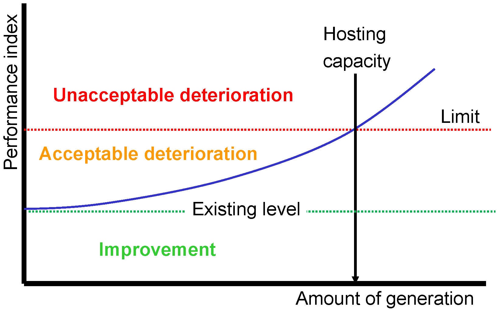
Figure 2.
Hosting capacity approach where the performance initially improves and only deteriorates with larger amounts of local generation.
Figure 2.
Hosting capacity approach where the performance initially improves and only deteriorates with larger amounts of local generation.

Figure 3.
Probability distribution (cumulative distribution function) for the highest voltage (worst-case voltage) for increasing amount of single-phase connected solar power in the 6-customer rural network. The different colours refer to the six different customers. The red dashed vertical line is the overvoltage limit at 110% of the nominal voltage.

Figure 4.
90th percentile of the worst-case overvoltage as a function of the number of customers with PV in the 6-customer rural network.
Figure 4.
90th percentile of the worst-case overvoltage as a function of the number of customers with PV in the 6-customer rural network.

Figure 5.
90th percentile of the worst-case overvoltage as a function of the number of customers with PV in the 6-customer rural network; 4 kW production per PV installation.
Figure 5.
90th percentile of the worst-case overvoltage as a function of the number of customers with PV in the 6-customer rural network; 4 kW production per PV installation.

Figure 6.
75th percentile of the worst-case overvoltage as a function of the number of customers with PV in the 6-customer rural network.
Figure 6.
75th percentile of the worst-case overvoltage as a function of the number of customers with PV in the 6-customer rural network.

Figure 7.
Probability distribution (cumulative distribution function) for the lowest voltage (worst-case voltage) for increasing amount of single-phase connected solar power in the 6-customer rural network. The different colours refer to the six different customers. The black dashed vertical line is the nominal voltage.

Figure 8.
Probability distribution (cumulative distribution function) for the highest voltage (worst-case voltage) for increasing amount of single-phase connected solar power in the 28-customer suburban network.
Figure 8.
Probability distribution (cumulative distribution function) for the highest voltage (worst-case voltage) for increasing amount of single-phase connected solar power in the 28-customer suburban network.
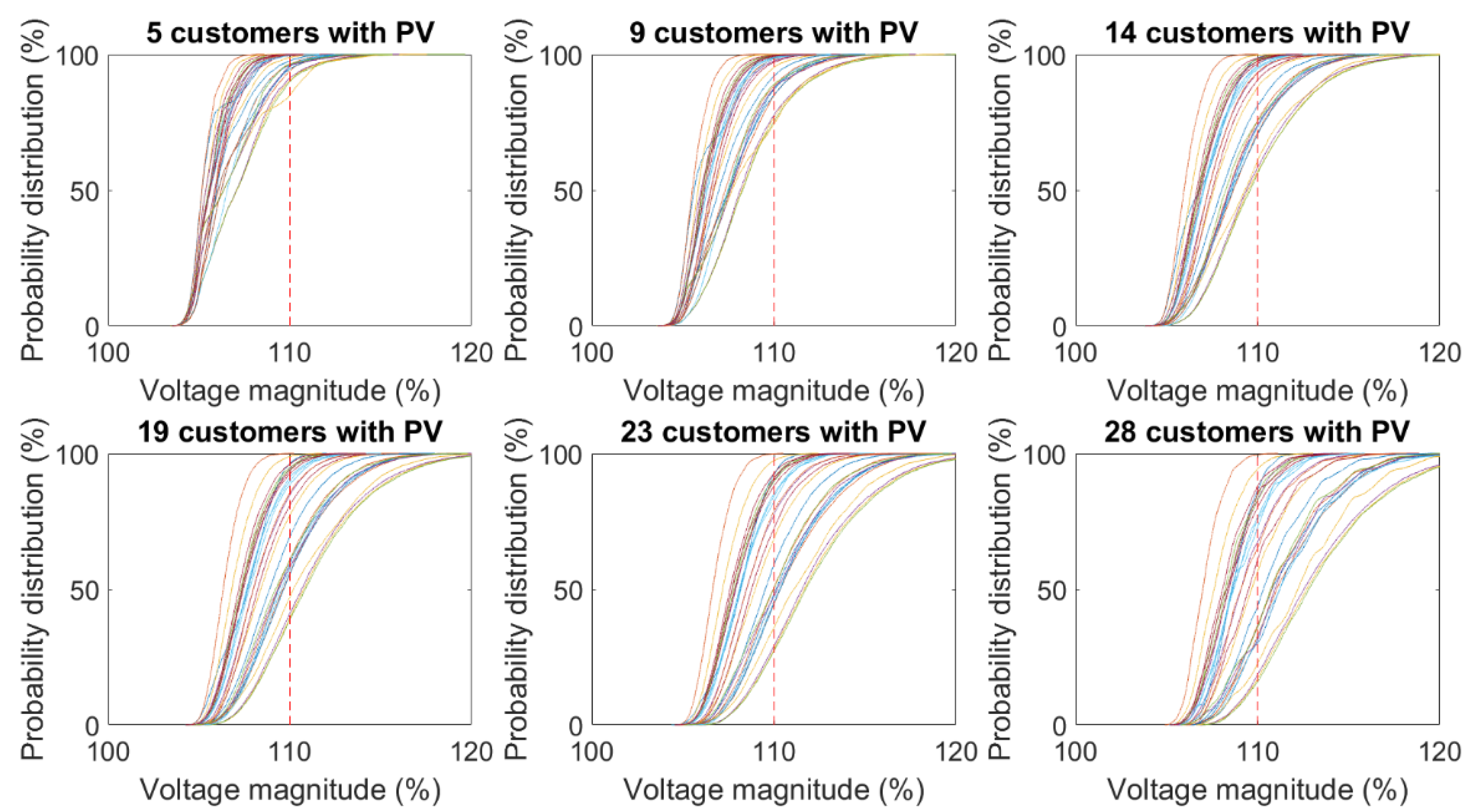
Figure 9.
90th percentile of the worst-case overvoltage as a function of the number of customers with PV in the 28-customer suburban network.
Figure 9.
90th percentile of the worst-case overvoltage as a function of the number of customers with PV in the 28-customer suburban network.

Figure 10.
10th percentile of the lowest voltage (worst-case voltage) as a function of the number of EV chargers in a 28-customer suburban network. A consumption of 5750 W (25 A) per charger has been used in the calculations.
Figure 10.
10th percentile of the lowest voltage (worst-case voltage) as a function of the number of EV chargers in a 28-customer suburban network. A consumption of 5750 W (25 A) per charger has been used in the calculations.

Figure 11.
Probability distribution (cumulative distribution function) of the highest single-phase current through the distribution transformer, with increasing number of customers with single-phase connected PV.
Figure 11.
Probability distribution (cumulative distribution function) of the highest single-phase current through the distribution transformer, with increasing number of customers with single-phase connected PV.
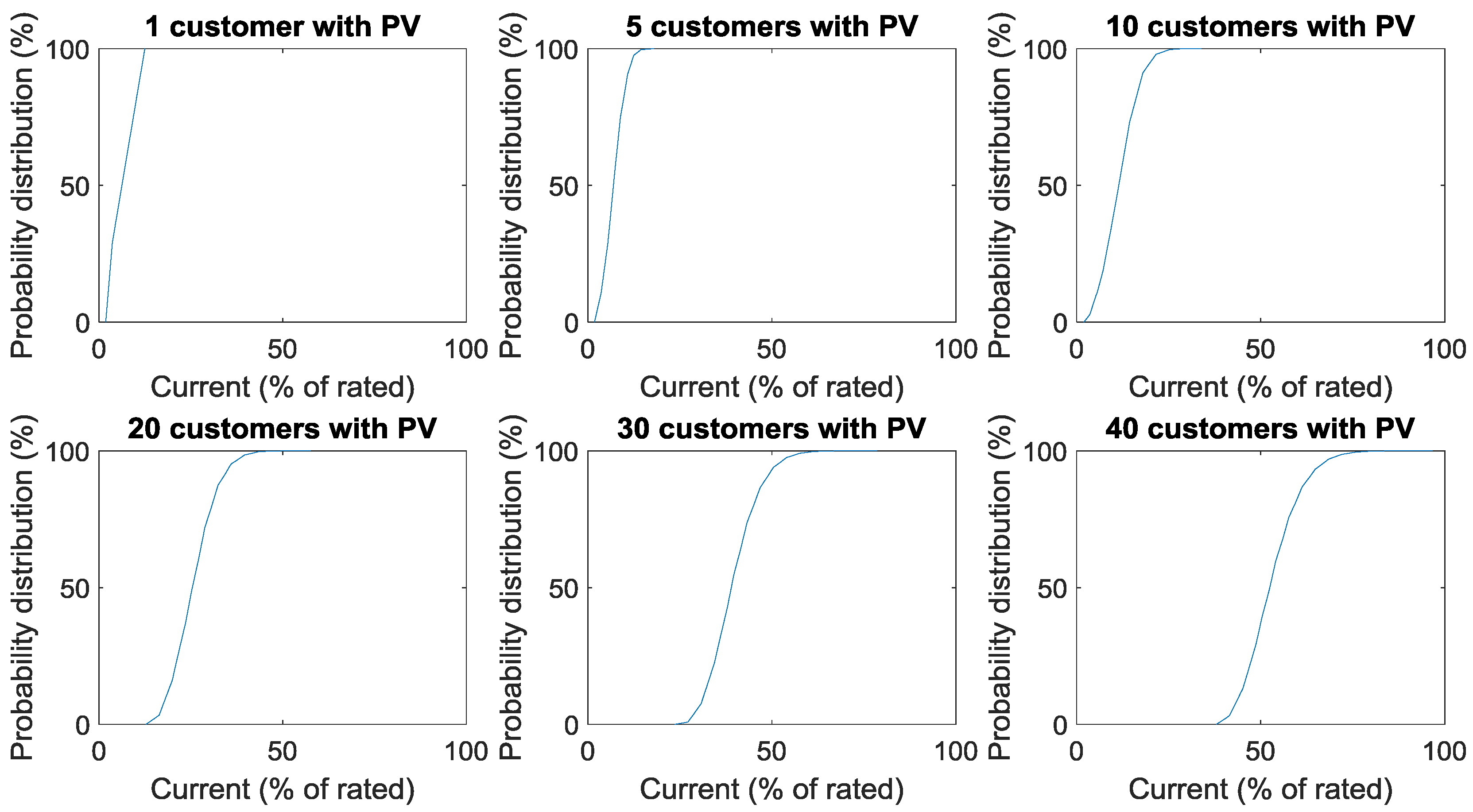
Figure 12.
Four different percentiles (50th: red star; 75th: green circle; 90th: blue plus; 95th: black triangle) for the current through the transformer, as a function of the number of customers (out of 83) with single-phase connected PV.
Figure 12.
Four different percentiles (50th: red star; 75th: green circle; 90th: blue plus; 95th: black triangle) for the current through the transformer, as a function of the number of customers (out of 83) with single-phase connected PV.

Figure 13.
Supraharmonics from a fluorescent lamp (left) and from a heat pump (right).

Figure 14.
Supraharmonics from a PV inverter connected alone (upper left), the same inverter while neighbouring devices are connected (upper right). A heat pump connected alone (lower left), the same heat pump while neighbouring devices are connected (lower right).
Figure 14.
Supraharmonics from a PV inverter connected alone (upper left), the same inverter while neighbouring devices are connected (upper right). A heat pump connected alone (lower left), the same heat pump while neighbouring devices are connected (lower right).


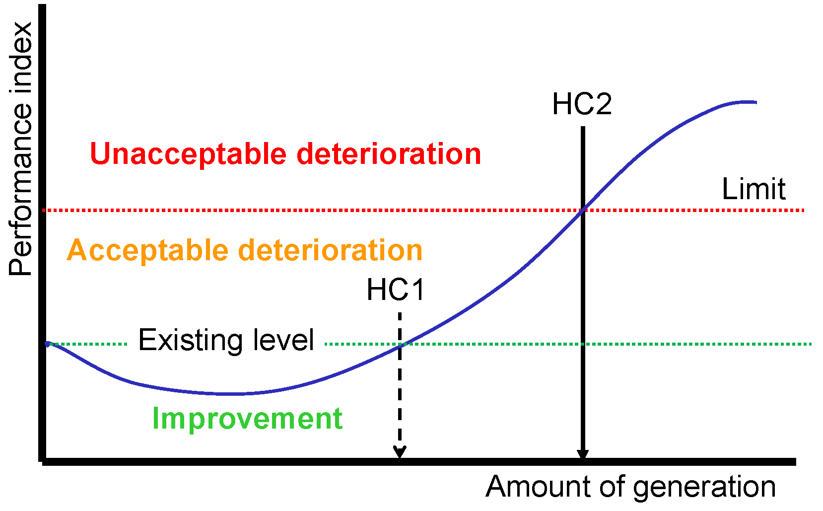
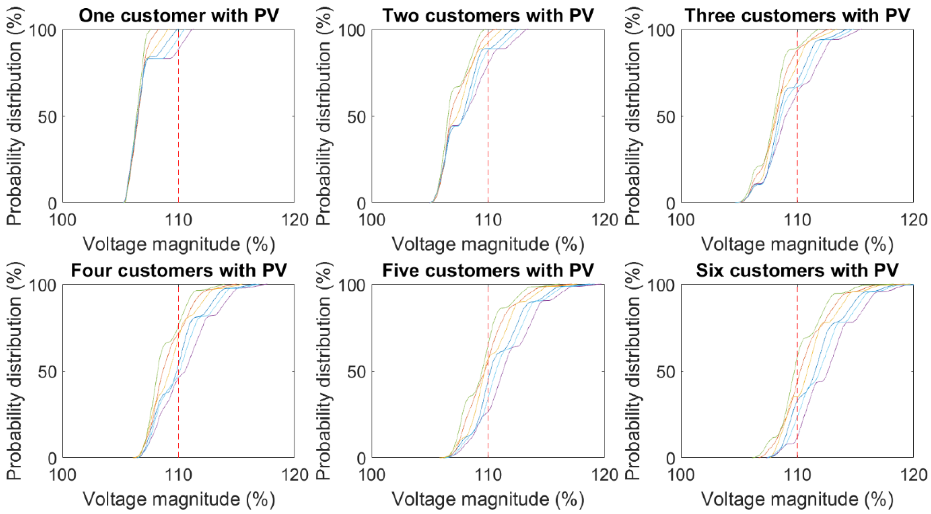
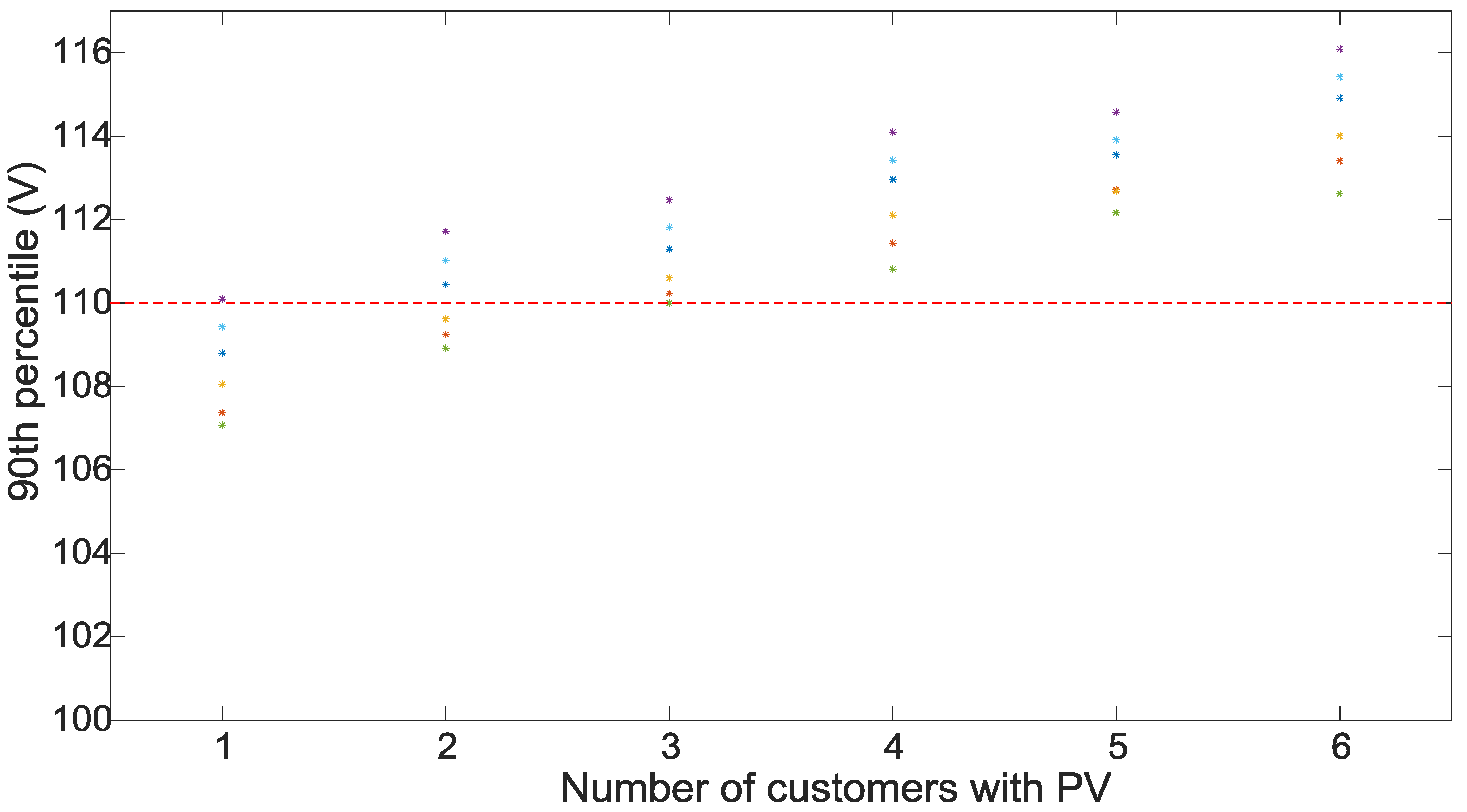
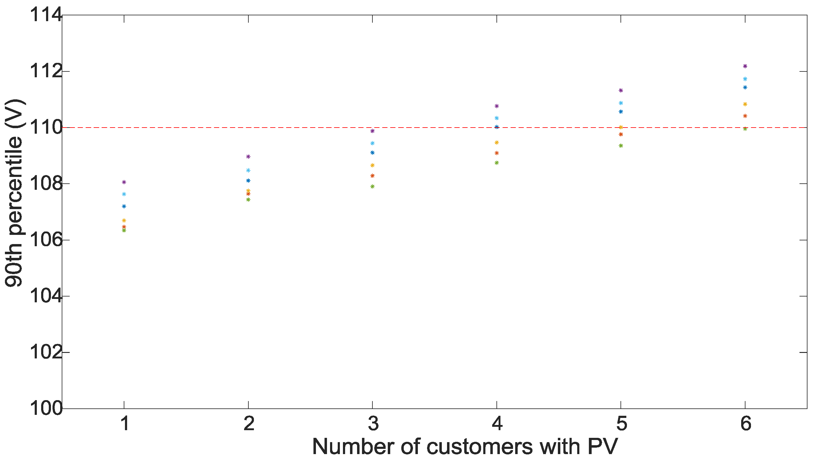
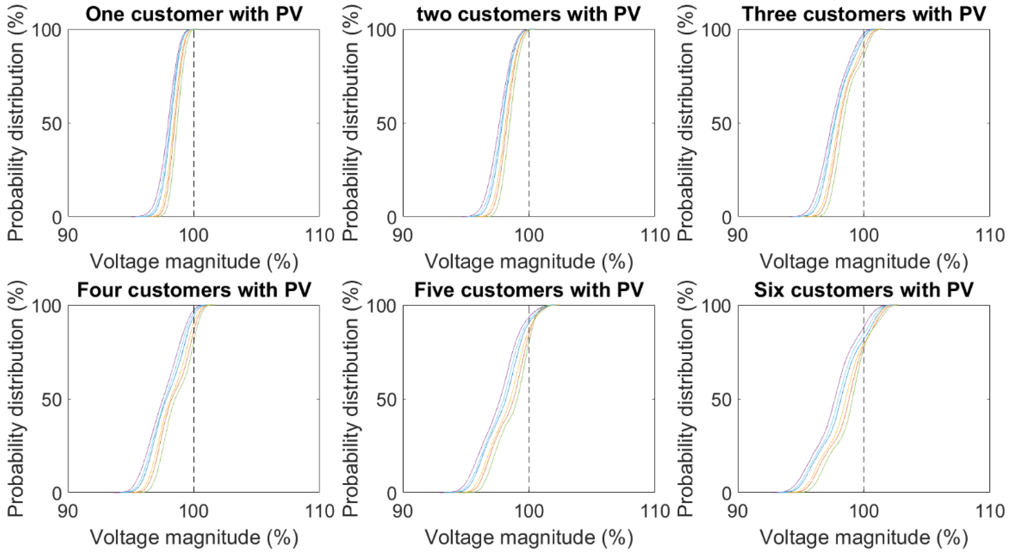
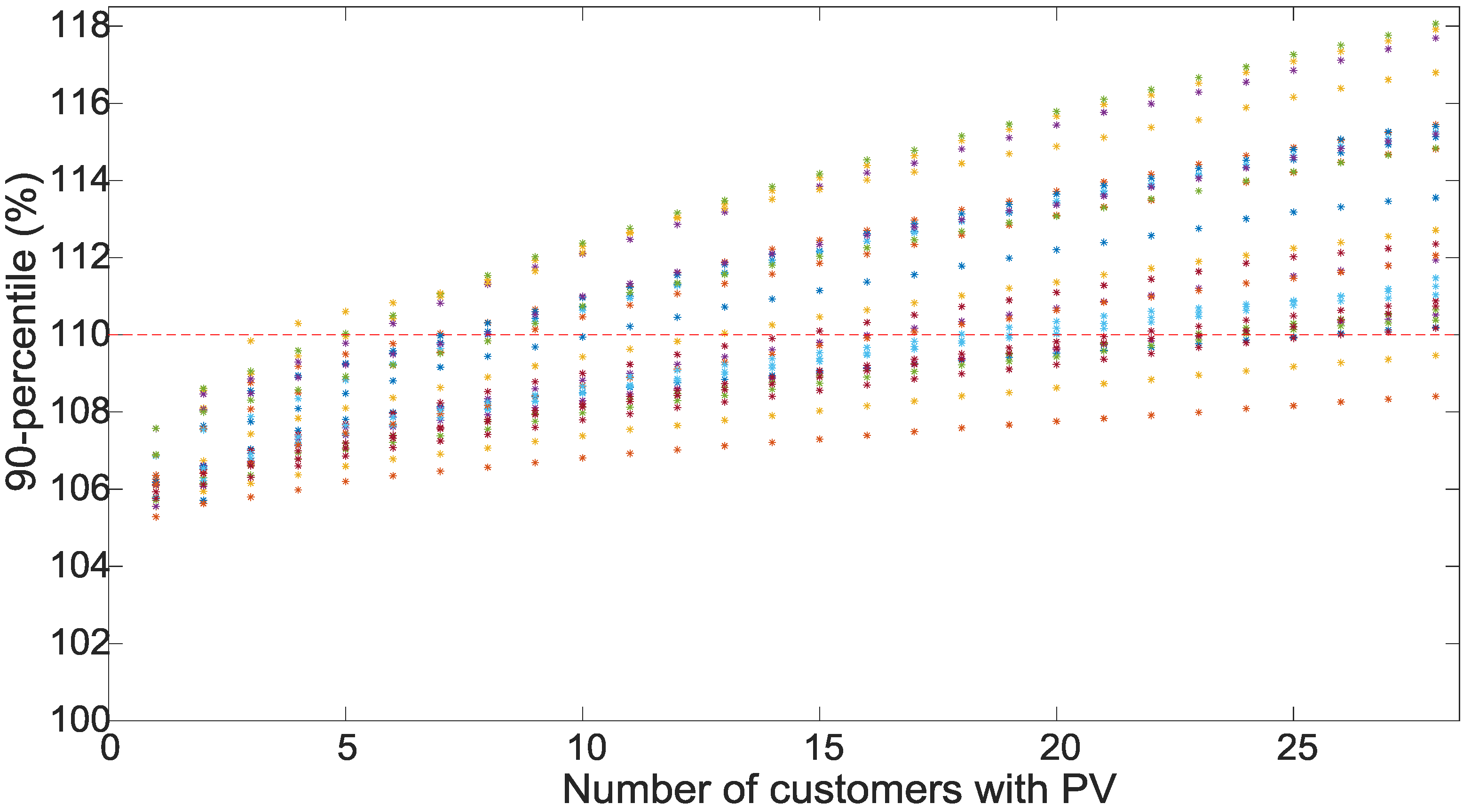
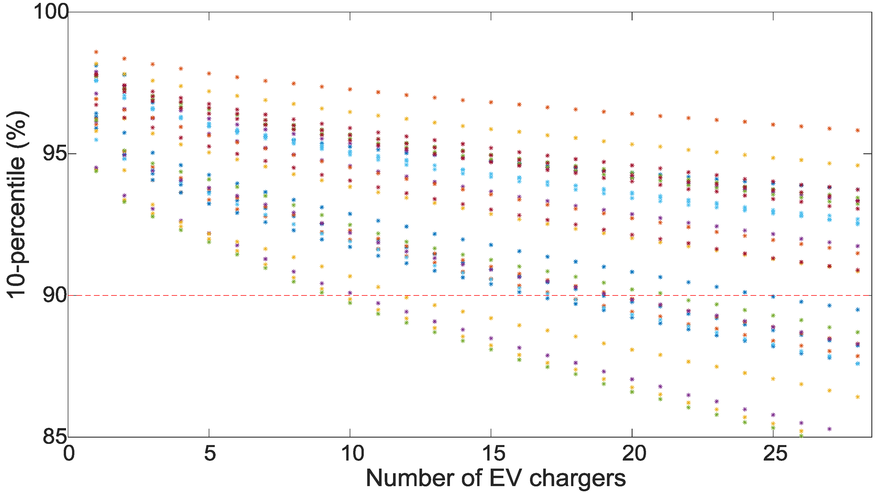
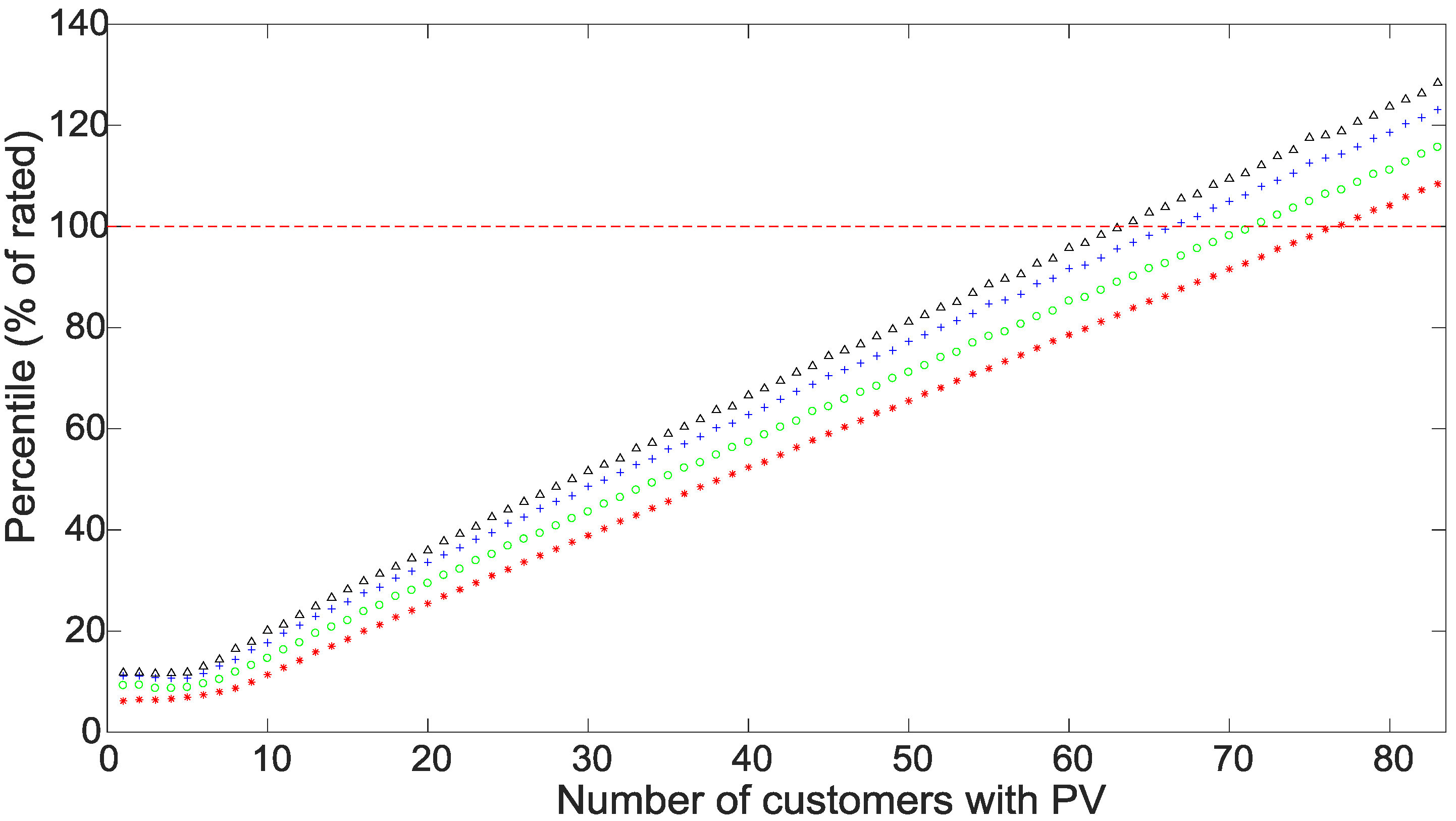
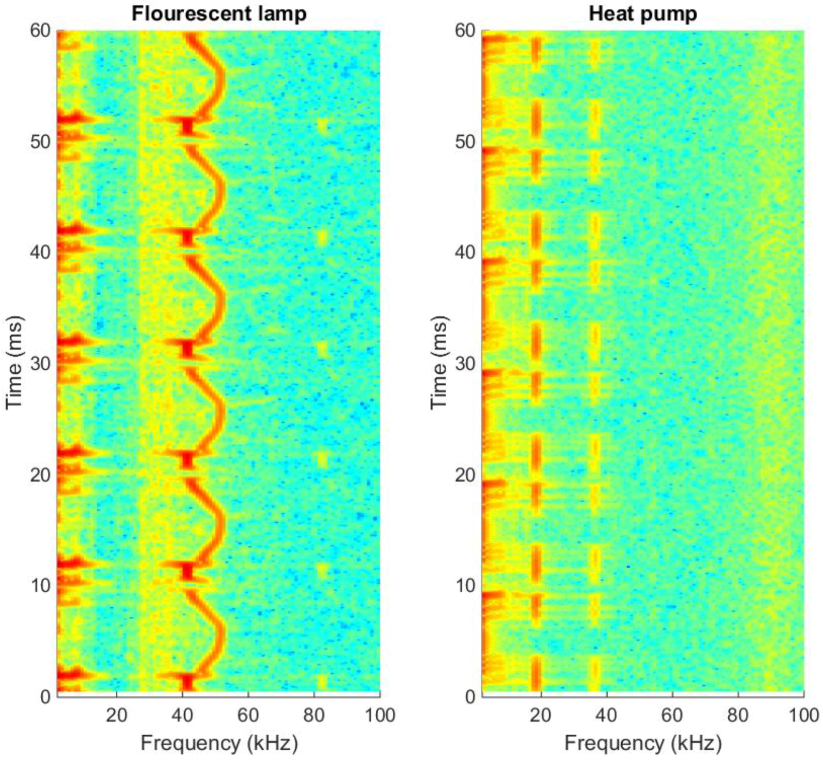
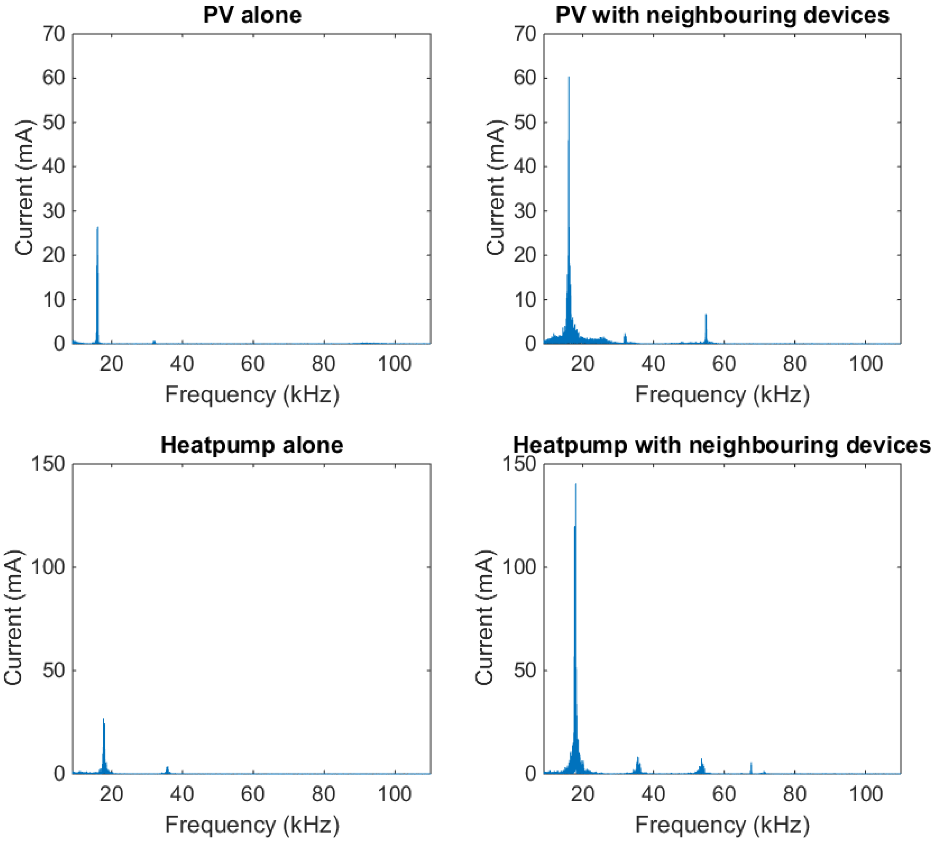
Table 1.
Sensitivity Analysis of the Hosting Capacity.
| Case | Parameter | Default Value | New Value | Hosting Capacity |
|---|---|---|---|---|
| 0 | 3 customers | |||
| 1 | Produced power per installation | 6 kW | 7 kW | 2 customers |
| 2 | 5 kW | 6 customers | ||
| 3 | 4 kW | 11 customers | ||
| 4 | Percentile | 90th | 95th | 1 customer |
| 5 | 85th | 5 customers | ||
| 6 | 75th | 8 customers | ||
| 7 | load per customer per phase | [0, 250 W] | [0, 150 W] | 3 customers |
| 8 | [0, 350 W] | 3 customers | ||
| 9 | No-load voltage | [238 V, 242 V] | [240 V, 244 V] | 2 customers |
| 10 | [239 V, 243 V] | 2 customers | ||
| 11 | [237 V, 241 V] | 4 customers | ||
| 12 | [236 V, 240 V] | 6 customers |
© 2017 by the authors. Licensee MDPI, Basel, Switzerland. This article is an open access article distributed under the terms and conditions of the Creative Commons Attribution (CC BY) license (http://creativecommons.org/licenses/by/4.0/).
Share and Cite
MDPI and ACS Style
Bollen, M.H.J.; Rönnberg, S.K. Hosting Capacity of the Power Grid for Renewable Electricity Production and New Large Consumption Equipment. Energies 2017, 10, 1325. https://doi.org/10.3390/en10091325
AMA Style
Bollen MHJ, Rönnberg SK. Hosting Capacity of the Power Grid for Renewable Electricity Production and New Large Consumption Equipment. Energies. 2017; 10(9):1325. https://doi.org/10.3390/en10091325
Chicago/Turabian StyleBollen, Math H. J., and Sarah K. Rönnberg. 2017. "Hosting Capacity of the Power Grid for Renewable Electricity Production and New Large Consumption Equipment" Energies 10, no. 9: 1325. https://doi.org/10.3390/en10091325
Note that from the first issue of 2016, this journal uses article numbers instead of page numbers. See further details here.