Icing Forecasting of Transmission Lines with a Modified Back Propagation Neural Network-Support Vector Machine-Extreme Learning Machine with Kernel (BPNN-SVM-KELM) Based on the Variance-Covariance Weight Determination Method

Abstract

Stable and accurate forecasting of icing thickness is of great significance for the safe operation of the power grid. In order to improve the robustness and accuracy of such forecasting, this paper proposes an innovative combination forecasting model using a modified Back Propagation Neural Network-Support Vector Machine-Extreme Learning Machine with Kernel (BPNN-SVM-KELM) based on the variance-covariance (VC) weight determination method. Firstly, the initial weights and thresholds of BPNN are optimized by mind evolutionary computation (MEC) to prevent the BPNN from falling into local optima and speed up its convergence. Secondly, a bat algorithm (BA) is utilized to optimize the key parameters of SVM. Thirdly, the kernel function is introduced into an extreme learning machine (ELM) to improve the regression prediction accuracy of the model. Lastly, after adopting the above three modified models to predict, the variance-covariance weight determination method is applied to combine the forecasting results. Through performance verification of the model by real-world examples, the results show that the forecasting accuracy of the three individual modified models proposed in this paper has been improved, but the stability is poor, whereas the combination forecasting method proposed in this paper is not only accurate, but also stable. As a result, it can provide technical reference for the safety management of power grid.

1. Introduction

Transmission line icing has a significant impact on the safe operation of power systems. In severe cases, it can even cause trips, disconnections, tower collapses, insulator ice flashovers, communication interruptions and other problems, which bring about great economic losses [1]. For example, a large cold wave area occurred in southeastern Canada and the northeastern United States in 1998, resulting in the collapse of more than 1000 power transmission towers, 4.7 million people couldn’t use electricity properly and the direct economic losses reached $5.4 billion [2]. In 2008, severe line icing accidents happened in South China, and caused forced-outages of 7541 10 KV lines and the power shortfall reached 14.82 GW [3]. The construction of a reasonable and scientific transmission line icing prediction model would be helpful for the power sector to deal with icing accidents in advance so as to effectively reduce the potential accident losses. Therefore, the study of icing prediction is of great practical significance and value.

In recent years, many scholars have been carrying out research on transmission line icing prediction. Some experts have developed sensor systems for direct measurement of icing events on transmission lines and they obtained real-time and intuitive icing thickness monitoring information [4,5,6]. However, the prediction accuracy of this method is poor, and this method is more suitable for collection equipment as raw data for it often needs icing model algorithms to predict the future icing trends. As a result, it is necessary to study model algorithms to predict icing thickness. Generally, the icing forecasting models can be divided into two categories, which include traditional models and modern intelligent models. Traditional models are further divided into two methods: physical models and statistical models. The physical prediction models are based on heat transmission science and fluid mechanics and other physics theories to analyze the icing thickness, such as Imai model [7], Goodwin model [8], Lenhard model [9], and hydrodynamic model [10]. However, icing is caused by many factors with too many uncertainties, which leads to the fact that the final forecasts provided by physical prediction models cannot live up to expectations. The statistical prediction models use the notion of mathematical statistics to predict the icing thickness based on icing records and extreme value theory. They include the time series model [11], extreme value model [12] and so on. However the application of statistical forecasting models needs to meet a variety of statistical assumptions, and they cannot consider the factors that influence icing thickness, which greatly limits the scope of application of the statistical models and improvement of the forecasting accuracy.

Therefore, it is more important to adopt the modern intelligent prediction models to predict transmission line icing with the development of big data, further research on artificial intelligence and constantly emerging optimization algorithms. Modern intelligent prediction models can handle nonlinear and uncertain problems scientifically and efficiently with computer technology and mathematical tools to improve prediction accuracy and speed. The back propagation neural network model and the support vector machine model are commonly-used intelligent models in the field of transmission line icing prediction. Li et al. [13] proposed a model based on BP neural networks for forecasting the ice thickness and the forecasting results showed that this model had good accuracy of prediction whether in the same icing process or in a different one. Wang et al. [14] put forward a prediction model of icing thickness and weight based on a BP neural network. The orthogonal least squares (OLS) method was used for the number of network hidden layer units and center vector so that the forecasting error could be controlled in a smaller range. However, the BP algorithm has a very slow convergence speed and it falls into local minima easily, so some scholars use the genetic algorithm and the particle swarm optimization to optimize the BP neural network. Zheng and Liu [15] proposed a forecast model based on genetic algorithm (GA) and BP, and the predication results proved that the GA-BP model was more effective than BP to forecast transmission line icing. Wang [16] structured a prediction model which used improved particle swarm optimization algorithm to optimize a normalized radial basis function (NRBF) neural network, and the training speed of the network was improved. In addition, some scholars used SVM to avoid the selection of neural network structure and local optimization problems, [17] and [18] built the icing prediction model based on a SVM algorithm with better accuracy, but the SVM algorithm is hard to implement for large-scale training samples, and there are difficulties in solving multiple classification problems, so some scholars have addressed these defects of SVM using the ant colony (ACO) [19], particle swarm (PSO) [19], fireworks algorithm (FA) [20] and quantum fireworks algorithm (QFA) [21]. Xu et al. [19] introduced a weighted support vector machine regression model that was optimized by the particle swarm and ant colony algorithms, and the proposed method obtained a higher forecasting accuracy. Ma and Niu [20] combined a weighted least squares support vector machine (W-LSSVM) with a fireworks algorithm to forecast icing thickness, which improved the prediction accuracy and robustness. Ma et al. [21] proposed a combination model based on the wavelet support vector machine (w-SVM) and the quantum fireworks algorithm (QFA) for icing forecasting.

GA, PSO, ACO and other algorithms are applied to advance the performance of BP neural networks and SVM, but these algorithms require a large initial population to solve large-scale optimization problems, and the solving efficiency and the ability to solve local optimization problems are still relatively general. Both the mind evolutionary computation (MEC) [22] and the bat algorithm (BA) [23] have high solving efficiency and strong competence in global optimization. Two new operators are added to MEC on the basis of genetic algorithm: convergence and dissimilation. They are responsible for local and global optimization, respectively, which greatly enhances the overall search efficiency and global optimization algorithm ability. The BA algorithm is a meta-heuristic algorithm proposed by Yang in 2010. Many scholars at home and abroad have studied the proposed algorithm, indicating that this algorithm takes into account both local and global aspects of solving a problem compared with other algorithms. In the search process, both of them can be interconverted into each other so that they can avoid falling into local optimal solutions and achieve better convergence.

As a new feed forward neural network, ELM can overcome the shortcomings of the traditional BP neural network and SVM. The algorithm not only reduces the risk of falling into a local optimum but also greatly improves the learning speed and generalization ability of the network. It has been applied in several prediction fields and obtained relatively accurate prediction results [24,25,26]. However, its prediction robustness is relatively poor due to the random initialization of the input weights and hidden layer bias characteristics, so Huang [27] proposed the kernel extreme learning machine algorithm (KELM) and thus overcame the weakness of poor stability and improved the algorithm precision.

The different forecasting methods reflect the change tendency of the object and its influencing factors from different aspects, respectively, and provide different information because of the respective principles, so any single forecasting method confronts the obstacle that the information is not comprehensive and the fluctuation of prediction accuracy is larger. Based on this, Bates and Granger [28] put forward the combination forecasting method for the first time in 1969 and it has achieved good results in many fields. For example, Liang et al. [29] proposed the optimal combination forecasting model combined the extreme learning machine and the multiple regression forecasting model to predict the power demand. The result indicated that this method effectively combined the advantages of the single forecasting models, thus its global instability was reduced and the prediction precision was satisfactory. Reference [30] introduced a combination model that included five single prediction models for probabilistic short-term wind speed forecasting and the proposed combination model generated a more reliable and accurate forecast. Few scholars have applied combination prediction methods in the field of the transmission line icing forecasting, so in this paper, we decided to adopt the combination forecasting method to predict line icing thickness. How to determine the weighted average coefficients of individual methods is the key problem. Compared to the arithmetic mean method [31] and induced ordered weighted averaging (IOWA) [32], the biggest advantage of the variance-covariance combined method [33] is that it can improve the robustness of prediction, which is more suitable for forecasting icing thickness.

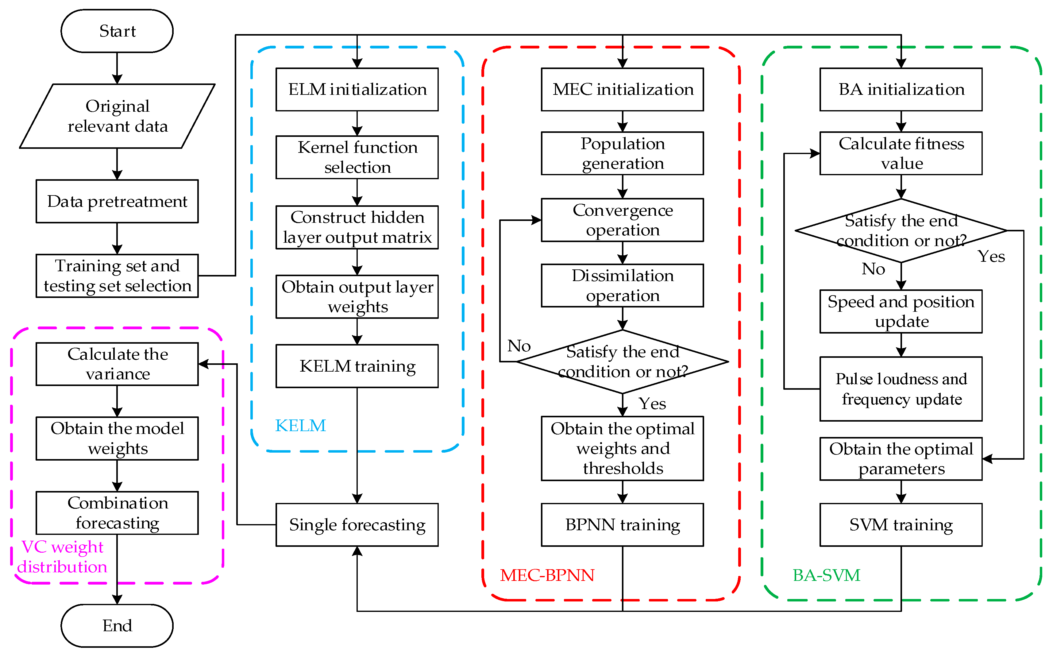
In summary, this paper adopts three models, including the BPNN optimized by the mind evolutionary algorithm (MEC-BPNN), the SVM optimized by the bat algorithm (BA-SVM) and the extreme learning machine with kernel based on single-hidden layer feed-forward neural network, to predict icing thickness using the historical icing thickness data and related meteorological data. The weighted average coefficients of individual forecasting methods are determined by a variance-covariance combined method to solve the problem of dynamic weight distribution. Then a modified BP-SVM-KELM combination forecasting model based on the VC combined method solving the problem of dynamic weight distribution method is constructed. The reason why we combine the three modified models is that their individual robustness is still poor, especially the BA-SVM and KELM. Furthermore, MEC-BPNN and KELM have the defects of underfitting and overfitting, respectively, and BA-SVM has difficulties dealing with large-scale training samples. Therefore, the combination model can give full play to the advantages of various prediction models, complement each other, and offer better robustness, stronger adaptability and higher prediction accuracy.

The rest of this paper is organized as follows: in Section 2, the MEC-BP, BA-SVM, KELM and VC combined method are presented in detail. Also, in this section, the integrated prediction framework is built. In Section 3, several real-world cases are selected to verify the robustness and accuracy of this model. In Section 4, another case is used to test the prediction performance of the proposed model. Section 5 concludes this paper.

2 Methodology

2.1. Mind Evolutionary Computation (MEC) to Optimize BPNN

MEC is a new evolutionary algorithm aiming at solving the defects of genetic algorithm and imitating the evolutionary process of human thinking. It inherits some ideas from the genetic algorithm and introduces two new operation operators, namely convergence and dissimilation, which are responsible for local and global optimization. The two operators are independent and coordinated, so improvement of any one can increase the whole search efficiency of the algorithm. Besides, there is strong ability of global optimization with a directed learning and memory mechanism. Using MEC to optimize the initial weights and thresholds of BPNN can make up for the defects that BPNN often falls into local optima and converges slowly. At present, MEC-BPNN is still rare in the field of the transmission line icing prediction though it has been widely used in other fields. The steps of using MEC to optimize the initial weights and thresholds of BPNN for forecasting are as follows:

(1)

Select the training set and test set. The training set is not only used for BPNN but also serves for the initialization of MEC. The test dataset is used for examining the model prediction accuracy. In order to make MEC-BPNN have good generalization performance, the training samples should be enough and representative.

(2)

MEC initialization. Set the population size of MEC, the number of superior races, the number of temporary population, the size of the sub-population, the number of iterations and the parameters of the BPNN interface.

(3)

Population generation. The initial population, superior sub-population and temporary sub- population are generated here serving for the convergent operation and dissimilation operation.

(4)

Convergence operation. The process of individuals’ competition for winners within a sub- population is called convergence. The end of the convergence process is the absence of winners within the population. That's a process of iteration.

(5)

Dissimilation operation. In the course of global competition among the sub-populations, if the score of a temporary sub-population is higher than that of a mature dominant population, the latter will be replaced and dissolved, or the former will be eliminated and disbanded. The new sub-population will be supplied with constant iteration.

(6)

Get the best individual. The MEC stops optimizing when the terminate condition of the iteration is reached. Then the optimal individual is parsed according to the encoding rules so that the weights and thresholds of the corresponding BPNN are obtained.

(7)

BPNN training. Set the initial input layer, hidden layer and output layer neuron number in initial settings of BPNN, and use the training set samples to train BP neural network with the optimized initial weights and thresholds.

(8)

Simulation prediction. Carry out the transmission lines icing forecasting if the simulation testing of the training result meets the expected goal, and to analyze the results.

2.2. Bat Algorithm (BA) to Optimize SVM

SVM is a machine learning algorithm based on statistical learning theory that can avoid the lack of learning ability of BPNN. SVM maps linear non-separable low dimensional space data into a linearly separable high-dimensional feature space by introducing a nonlinear inner product kernel function and the classification or regression fitting is carried out in this space. The regression fitting of SVM is called support vector regression (SVR). In this paper, ε-SVR is used to study the nonlinear icing thickness prediction. The nonlinear SVR needs to map the raw data into high-dimensional feature space by kernel function, and then apply linear regression in high-dimensional feature space. The specific algorithm flow of ε-SVR refers to the reference [34].

The selections of the penalty parameter c, kernel function parameter g and ε loss function parameter p are crucial because the prediction performance of SVM is influenced by these key parameters. Compared with other algorithms, the global optimization ability of BA is stronger, and it can avoid falling into local optimization. Therefore, this paper adopts BA algorithm to optimize the three key parameters.

The bat algorithm is a new intelligent optimization algorithm inspired by the echo localization of micro bats in nature. In nature, most bats use echolocation method to hunt their prey, and they can emit dozens of sounds at up to 110 dB ultrasonic pulses per second. When the bats come near the prey, the pulse intensity decreases and frequency increases. Bats usually produce higher frequency sound waves and wider bands for hunting prey in complex environments. If the bat is simulated as agent in the search space, the good or bad of the agent’s position is measured by the quality of objective functions, and the process of bats finding prey is just like the process of searching for the optimal solution in solution space. Then the behavior of bats using ultrasonic positioning can be described using the following equations. Suppose the bat population is n, the speed and position of the bat i are updated according to Equations (2) and (3):

$$f_i=f_{\min }+(f_{\max }-f_{\min })\alpha$$

(1)

$$v_i^t=v_i^{t-1}+(l_i^{t-1}-l_{\ast })f_i$$

(2)

$$l_i^t=l_i^{t-1}+v_i^t$$

(3)

where f_i is the frequency of sound waves generated by the i bat; f_min and f_max are the minimum and maximum frequency of sound waves respectively; $\alpha$ is a random number within [0, 1]; $v_i^{t-1}$ and $v_i^t$ are the velocity at time t−1 and the time t of the i bat; $l_i^{t-1}$ and $l_i^t$ are the position at time t−1 and the time t of the i bat; l_∗ is the position of the bat when the target function is optimal in the current global search. In the initialization process, each bat should be assigned a random frequency, but the frequency should be within the set range. In the local search, the position of the bat is updated according to the new formula if a solution is selected from the optimal set:

$$l_{new}=l_{old}+\epsilon A^t$$

(4)

where ε is a random number within [0, 1]; A^t is the average loudness of all bats at time t; l_old is a solution that is randomly selected from the set of optimal solutions.

The pulse loudness A_i and frequency R_i emitted by i bat will change continuously. During searching, for example, A_min = 0 indicates that the bat has discovered the prey at this time and pauses the ultrasonic wave; A_max = 10 indicates that bats increase the pulse loudness as much as possible to obtain more information in order to search for prey. Pulse loudness and pulse frequency can be updated by Equations (5) and (6):

$$A_i^{t+1}=\tau A_i^t$$

(5)

$$R_i^{t+1}=R_i^0[1-e^{-\gamma t}]$$

(6)

where the value of the pulse loudness increasing coefficient $\tau$ and pulse frequency attenuation coefficient are selected according to the subjects. The range of $\tau$ is in [0, 1]; γ > 0. The optimal solution is similar to the prey of the bat in BA algorithm, and the variation of pulse loudness and frequency represents, to some extent, the closeness to the optimal solution.

The fitness function used by the BA algorithm is the root-mean-square error (RMSE) under k-fold cross validation (K-CV). The RMSE can be obtained by Equation (22). K-CV randomly divides the training samples into k disjoint subsets, each of which is roughly equal in size. Using k-1 training subsets, a regression model is established for a given set of parameters, and the RMSE of the remaining last subset is used to evaluate the performance of the parameters. Repeat the procedure K times, and each subset has the opportunity to be tested. The accuracy of cross validation is the average value of the percentage of data correctly predicted for K times. The expected generalization error is estimated according to the average value of RMSE obtained after the K iteration, and finally a set of optimal parameters is selected [35].

2.3 Extreme Learning Machine with Kernel (KELM)

ELM was put forward by Huang et al. in 2006. Based on this theory, the basic extreme learning machines, online sequential extreme learning machines and KELM algorithms have been derived [36]. KELM is a single layer feedforward neural network algorithm. Compared with ELM, its ability to solve regression prediction is stronger, and compared with BPNN and SVM, its calculation speed is faster when the prediction accuracy is better or similar, which greatly improve the generalization ability of network [37]. The KELM algorithm has been proved to have excellent forecasting performance in many fields.

First, the neural network construction mechanism of the basic ELM algorithm is briefly described, and its neural network function is shown as follows:

$$g(x)=h_i(x)\cdot {\beta }_i$$

(7)

where g(x) is the network output value, h_i(x) is the output of the i hidden layer neurons which corresponds to the input x; ${\beta }_i$ is the connection weights between the i hidden layer neurons and the output neurons.

ELM’s precision of regression forecasting is guaranteed by minimizing the output error as follows:

$$\underset{L\to \infty }{\lim }\Vert g(x)-g_O(x)\Vert =\underset{L\to \infty }{\lim }\Vert {\displaystyle \sum _{i=1}^L{\beta }_i{h}_i(x)-}{g}_O(x)\Vert =0$$

(8)

where L is the number of neurons in the hidden layer; g_O(x) is the predictive function of the target value.

At the same time, the ELM algorithm guarantees the generalization ability of neural networks by minimizing the output weight β. The β usually takes its least square solution, and the calculation method is shown as follows:

$$\begin{array}{cc}\hfill \beta & =H^{+}O=H^T{(H{H}^T)}^{-1}O\hfill \\ & =H^T{(\frac{1}{C}+H{H}^T)}^{-1}O\hfill \end{array}$$

(9)

where H is the hidden layer matrix of neural network; H⁺ is the generalized inverse matrix of H matrix; O is predictive target vector. According to ridge regression theory, the results will be more stable and provide better generalization ability by increasing the normal number 1/C.

The KELM algorithm introduces the kernel function for obtaining better regression prediction accuracy. The kernel matrix is defined by applying Mercer' s condition as follows:

$$\{\begin{array}{l}{\mathsf{\Omega }}_{\mathrm{ELM}}=H{H}^T\\ {\mathsf{\Omega }}_{i,j}=h(x_i)\cdot h(x_j)=K(x_i,x_j)\end{array}$$

(10)

The random matrix HH^T of ELM is replaced by the kernel matrix $\mathsf{\Omega }$, then all the input samples are mapped from the n-dimensional input space to a high dimensional implicit feature space by kernel function. The mapping value of the kernel matrix $\mathsf{\Omega }$ is fixed after setting the nuclear parameter. The kernel functions include Radical Basis Function (RBF) kernel functions, linear kernel functions and polynomial kernel functions. It is usually set as RBF kernel, and the formula is as follows:

$$K(\mu ,\nu )=\exp [-(\mu -{\nu }^2/\sigma )]$$

(11)

The parameter 1/C is added to the main diagonal of the unit diagonal HH^T so that the eigenvalues is not 0, and then the weight vector β* is obtained. It makes ELM more stable and has better generalization. The output weight of the ELM network here is as follows:

$${\beta }^{\ast }=H^T{(I/C+H{H}^T)}^{-1}O$$

(12)

where I is diagonal matrix; C is penalty coefficient for weighing the proportion between structural risk and empirical risk; HH^T is generated by mapping input samples from kernel functions.

From the above formulas, the output of the KELM model is described as follows:

$$\begin{array}{cc}\hfill f(x)& =h(x)H^T{(I/C+H{H}^T)}^{-1}O\hfill \\ & ={\left[\begin{array}{c}K(x,x_1)\\ ⋮\\ K(x,x_N)\end{array}\right]}^T{(I/C+{\mathsf{\Omega }}_{ELM})}^{-1}O\hfill \end{array}$$

(13)

In the KELM algorithm based on kernel, the specific form of feature mapping function h(x) of hidden nodes is not given specially, and the output function value can be obtained only by the concrete form of kernel function. In addition, since the kernel function uses the inner product directly, it is unnecessary to set the number of hidden layer nodes when solving the output function value, so the initial weight and bias of hidden layer needn’t be set.

2.4. VC Combined Method Solved the Problem of Dynamic Weight Distribution

The combination forecasting model can integrate the advantages of each single model and improve the prediction precision. The merit of VC combined method solved the problem of dynamic weight distribution is that the optimum combination weight coefficient can be found, so the robustness and accuracy can be improved.

The variance of each prediction model is calculated by the following formula:

$${\delta }_i=\frac{1}{n}\cdot \left[{(e_1-\overline{e})}^2+{(e_2-\overline{e})}^2+\cdots +{(e_n-\overline{e})}^2\right]i=1,2,3$$

(14)

where n is the number of training samples; e₁, e₂, …, e_n are the absolute percentage error for each training sample; $\overline{e}$ is the average absolute percentage error of the n training sample.

The weights are derived from the variance according to the following formula:

$${\omega }_1=1/\left[{\delta }_1(1/{\delta }_1+1/{\delta }_2+1/{\delta }_3)\right]$$

(15)

$${\omega }_2=1/\left[{\delta }_2(1/{\delta }_1+1/{\delta }_2+1/{\delta }_3)\right]$$

(16)

$${\omega }_3=1/\left[{\delta }_3(1/{\delta }_1+1/{\delta }_2+1/{\delta }_3)\right]$$

(17)

The weights are multiplied by the corresponding prediction results, and the combined prediction results are shown as follows:

$$g={\omega }_1{g}_1+{\omega }_2{g}_2+{\omega }_3{g}_3$$

(18)

where g is the combined forecasting result; g₁, g₂ and g₃ are the individual prediction results of each model. The result of the combination is that the corresponding weights are adjusted dynamically with the different training and test results for better adaptability.

2.5. Combination Forecasting Model

Firstly, the original relevant data is selected and preprocessed, after which the data is divided into test samples and training samples. Then, three single modified models are utilized to forecast respectively, including MEC-BP, BA-SVM and KELM. Finally, the forecasting results are combined by VC combined method solving the problem of dynamic weight distribution. The proposed combination forecasting model is shown in Figure 1.

3. Case Study and Results Analysis

3.1 Data Selection

There are many factors affecting the transmission line icing thickness. According to [38], the temperature, relative air humidity, wind speed and wind direction are the major factors. The temperature must be less than or equal to 0 °C. If the relative air humidity is above 85%, it is easier for icing to occur on transmission lines. When the icing temperature and vapor conditions are present the wind plays an important role in the icing of the wires. It can deposit large amounts of supercooled water droplets continuously onto the lines, and then collide with the wire and gradually increase these deposits to cause icing phenomens. It is observed that icing first grows on the windward side of the line, and the wire is twisted due to gravity when the windward side reaches a certain icing thickness, so a new windward surface appears. In this way, the icing gradually increases by constantly twisting, and eventually circular or elliptical icing is formed, so the wind speed should exceed 1 m/s in the process. In addition, the wind direction also affects the lines’ icing. The angle of wind direction is measured by taking the direction of the wire as the benchmark, i.e., the direction of the wire is set to be horizontal 0°. When the wind rotates counterclockwise around the wire, if the angle between the wind and the wire is in the range of [0°, 180°), the closer the angle is to 0° or 180°, the lighter the icing degree is, and the closer the angle is to 90°, the more serious the degree of icing is, or the closer the angle is to 180° or 360°, the lighter the icing degree is, and the closer the angle is to 270°, the more serious the degree of icing.

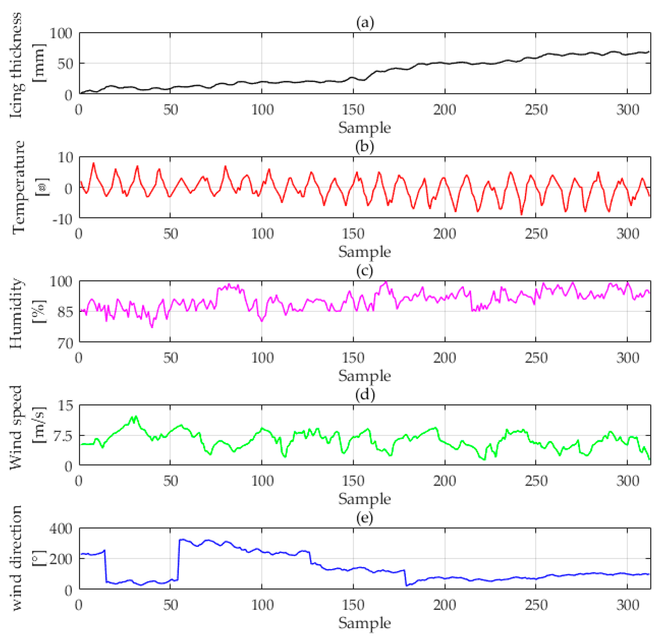
Affected by the abnormal atmospheric circulation and La Niña weather patterns, cold air entered Hunan in 11 January 2008 making the area cool rapidly. The strength of the frontal inversion formed by the confluence of cold and warm air was great. What’s more, the terrain in Hunan is lower in the north and higher in the south, which made the strength of the frontal inversion greater. The stronger the strength of the frontal inversion, the stronger the strength of the rain and snow, so a continuous glaze was formed with the continuous supplement of warm wet air, and Hunan power grid suffered a record disaster accompanied by a large area of rain and snow, freezing rain incidents and large scale icing of transmission lines and substations. During the freezing disaster, the number of collapsed transmission towers reached 2242 and the number of deformed transmission towers reached 692, causing serious damage to the power grid. Therefore, we selected the "Dong-Chao line" of Hunan, which was the hardest-hit area during the Chinese icing incident in 2008 as a case study to verify the effectiveness of the proposed model. The example chooses some data including the transmission lines icing thickness, regional temperature, relative air humidity, wind speed and wind direction from 0:00 12 January 2008 to 24:00 6 February 2008. Here we take 2 h as the data collection frequency, and each indicator collects 312 sets of data where the first 192 are used as the training samples and the latter 120 are test samples in Case 1.

The original data is shown in Figure 2. All of the data were provided by Key Laboratory of Disaster Prevention and Mitigation of Power Transmission and Transformation Equipment (Changsha, Hunan Province, China), where all the data are collected by professional instruments and can reflect the state changes during the icing process. As we can see from Figure 2, the temperature and wind speed data present a cyclical downward trend, while the relative air humidity data present a cyclical upward trend. In addition, there is no exceptional data or missing data. Hence these data can be used directly as data sources.

In addition to the icing thickness, the data of temperature, relative air humidity, wind speed and wind direction at the forecast point T was selected as input data. However, ice accretion phenomenon is a continuous process and the prior T-z’s icing thickness can influence the transmission lines icing thickness at the forecast point T. When selecting the different prior T-z’s icing thickness as input data, the forecasting effectiveness is different. Hence this paper selects different prior T-z’s icing thicknesses as input data. For example, when z equals 3, the input icing thickness data includes the icing thickness at T-1, T-2, and T-3. After selecting the input data, the proposed model is applied to check the exact input icing thickness by using the training samples, whose experimental results are shown in

Table 1. RMSE of proposed model when selecting the input icing thickness data at different time point.

z	1	2	3	4	5
RMSE of Proposed Model	0.0321	0.0201	0.0156	0.0115	0.0115
z	6	7	8	9	10
RMSE of Proposed Model	0.0115	0.0115	0.0115	0.0115	0.0115

.

From Table 1, it can be found that the proposed model obtains different error values when the icing thickness values are selected at different time points. However when z equals 4, the RMSE of proposed model reaches the minimum value, thus the input icing thickness data includes the icing thickness at T-1, T-2, T-3 and T-4, while the other input data includes the temperature, relative air humidity, wind speed and wind direction at the forecast point T.

3.2. Data Pretreatment

The data preprocessing steps are as follows:

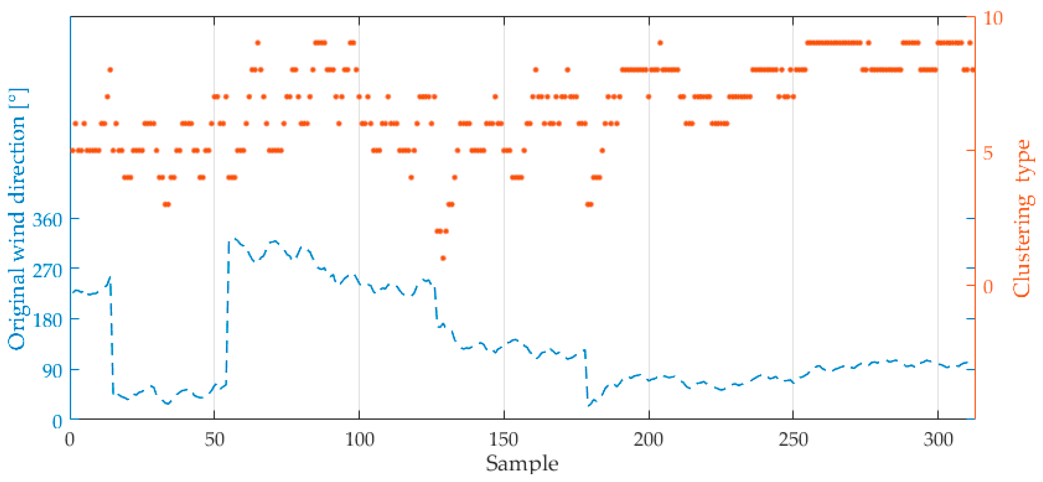
(1) Wind direction data clustering processing

The large fluctuation range of wind direction data will reduce the accuracy of prediction results, and the clustering of wind direction data can make the fluctuation smaller which can improve the prediction accuracy. Thus, the paper uses clustering to process wind direction data according to the degree of influence of wind direction on icing thickness; which formula is as follows:

$$J=\{\begin{array}{cc}ceil(0.1\theta ),\hfill & 0\le \theta <90\hfill \\ ceil(18-0.1\theta ),\hfill & 90\le \theta <180\hfill \\ ceil(0.1\theta -18),\hfill & 180\le \theta <270\hfill \\ ceil(36-0.1\theta ),\hfill & 270\le \theta <360\hfill \end{array}$$

(19)

where J is the result value of clustering process for wind direction; θ is the angle between the wind and the wire when the wind rotates counterclockwise around the wire, i.e., the direction of the transmission line is set to be horizontal 0°; Ceil is the bracket function. The wind direction processing data for "Dong-Chao line" is shown in Figure 3.

(2) Standardized processing of all data

Due to the different nature of each evaluation index, and they usually have different dimensions and orders of magnitude. In order to ensure the accuracy of the prediction results, it is necessary to standardize the original index data. The data are processed by the following equation:

$$Z=\left\{z_i\right\}=\frac{x_i-x_{\min }}{x_{\max }-x_{\min }}i=1,2,3,\dots ,n$$

(20)

where x_i is actual value and the actual value of wind direction data is the result of clustering; x_min and x_max are the minimum and maximum values of the sample data.

3.3. Performance Evaluation Index

The evaluation index of the icing prediction result used in this paper are:

(1)

Relative error (RE):

$$\mathrm{RE}=\frac{x_i-{\widehat{x}}_i}{x_i}\times 100\%$$

(21)

(2)

Root-mean-square error (RMSE):

$$\mathrm{RMSE}=\sqrt{\frac{1}{n}{\displaystyle \sum _{i=1}^n{(\frac{x_i-{\widehat{x}}_i}{x_i})}^2}}$$

(22)

(3)

Mean Absolute Percentage Error (MAPE):

$$\mathrm{MAPE}=\frac{1}{n}{\displaystyle \sum _{i=1}^n\left|(x_i-{\widehat{x}}_i)/x_i\right|}\cdot 100\%$$

(23)

(4)

Average absolute error (AAE):

$$\mathrm{AAE}=\frac{1}{n}({\displaystyle \sum _{i=1}^n\left|x_i-{\widehat{x}}_i\right|})/(\frac{1}{n}{\displaystyle \sum _{i=1}^n{x}_i})$$

(24)

where $x$ is the actual value of the icing thickness; $\widehat{x}$ is the forecasting value; $n$ is groups of data. The smaller the above index value is, the higher the prediction accuracy is.

3.4. Modified BPNN-SVM-KELM for Icing Forecasting

The paper’s experiment and modeling platform is Matlab R2014a, and the operating environment is an Intel Core i5-6300U CPU with 4G memory and a 500 G hard disk. The topology structure of BPNN in MEC-BPNN is 9-7-1. The transfer function of the hidden layer uses the expression $f(x)=2/(1+e^{-2x})-1$ which is a tansig function. The output layer transfer function takes the form $f(x)=x$ which is a purelin function. The maximum training time is 100, the training target minimum error is 0.0001, and the training speed is 0.1. In addition, the population size of MEC is 200, the sub-population is 20, the dominant sub-population’s number is 5, the quantity of the temporary population is 5, the number of iterations is 10. The parameters of the BA algorithm in the BA-SVM prediction are set as follows: the dimension of search space is 7; the size of the bat population is 30; the pulse frequency R_i of bats is 0.5; loudness A_i is 0.25; the acoustic frequency range is [0, 2]; the termination condition of the algorithm is when the calculation reaches the maximum number of iterations (300). In SVM, the penalty parameter that needs to be optimized is C whose range of variation is [0.01, 100]; the range of kernel parameter g is [0.01, 100]; the range of the ε loss function parameter p is set as [0.01, 100]. The SVM optimal penalty parameter c is 1.971, the kernel parameter g is 0.010 and the ε loss function parameter p is 0.01 by BA optimization. The kernel function of KELM algorithm uses RBF kernel function whose input and output data processing interval is [−1, 1].

In order to show whether the forecasting results of the three modified models were a local optimal or global optimal location and whether these models can be generalized to other unseen data, a K-CV test is conducted here. According to the K-CV method described in Section 2.2, the data set is substituted into the model for testing and analysis. The 312 sets of data are randomly divided into 12 datasets, each of which has 26 groups of data and do not intersect each other. After 12 operations, each sub-data set is tested and the RMSE of the sample is obtained, which can be seen in the

Table 2. Results of the k-fold cross validation.

Fold Number	RMSE of MEC-BPNN	RMSE of BA-SVM	RMSE of KELM
1	0.0126	0.0132	0.0136
2	0.0131	0.0205	0.0142
3	0.0126	0.0141	0.0135
4	0.0112	0.0126	0.0128
5	0.0118	0.0139	0.0142
6	0.0139	0.0149	0.0151
7	0.0143	0.0152	0.0137
8	0.0125	0.0133	0.0132
9	0.0101	0.0124	0.0152
10	0.0117	0.0128	0.0139
11	0.0109	0.0151	0.0149
12	0.0102	0.0118	0.0122
Average Value	0.0121	0.0142	0.0139
Standard Deviation	0.00129	0.00219	0.00087

.

From Table 2, it can be known that the average RMSE values of MEC-BPNN, BA-SVM and KELM are 0.0121, 0.0142 and 0.0139, respectively. The RMSE standard deviations of MEC-BPNN, BA-SVM and KELM are 0.00129, 0.00219 and 0.00087, respectively. It is indicated that the validation error of the each modified model proposed in this paper can obtain its global minimum.

After the prediction of the three individual improved models, the VC combined method to solve the problem of dynamic weight distribution is adopted to combine these models. The result of the combination is that the corresponding weights are adjusted dynamically according to the different training results whose adaptability is better. The combination weights of three individual models of MEC-BPNN, BA-SVM and KELM are 0.42, 0.34 and 0.24, respectively.

The paper uses the mature BP neural network model and SVM model to do a comparative experiment based on the sample data mentioned in Section 3.1 in order to verify the performance of the proposed combination forecasting model. The initial weights and thresholds of a single BPNN model are obtained by their own training, and other parameter settings are consistent with the MEC-BPNN. Besides, in the single SVM model, the penalty parameter c is 9.063, the kernel function parameter g is 0.256, and the ε loss function parameter p is 3.185.

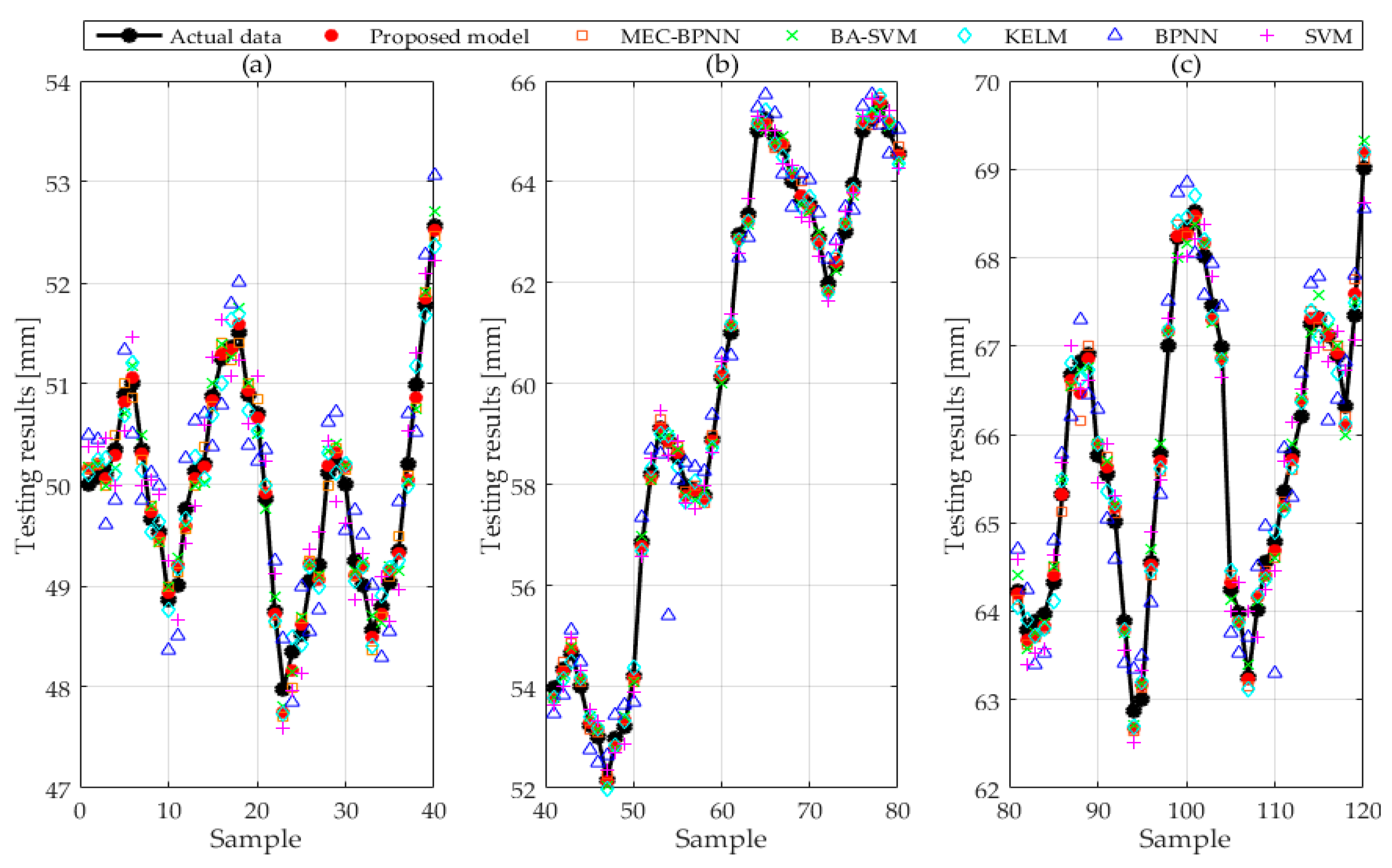
The forecasting values and original values of BPNN, SVM, MEC-BPNN, BA-SVM, KELM, and improved BP-SVM-KELM based on VC, part of which are given in

Table 3. Part of the forecasting value and relative errors of each model.

Data Point Number	Actual Value (mm)	BPNN		SVM		MEC-BPNN		BA-SVM		KELM		Proposed Model
		Forecast Value	Error %	Forecast Value	Error %	Forecast Value	Error %	Forecast Value	Error %	Forecast Value	Error %	Forecast Value	Error %
1	50.01	50.5	0.98	50.38	−0.74	50.17	−0.32	50.18	−0.34	50.11	−0.20	50.16	−0.30
2	50.08	50.45	−0.74	50.38	−0.60	50.2	−0.24	50.2	−0.24	50.25	−0.34	50.21	−0.26
3	50.11	49.61	1.00	50.47	−0.72	50	0.22	50	0.22	50.27	−0.32	50.07	0.09
4	50.35	49.85	0.99	50	0.70%	50.5	−0.30	50.16	0.38	50.11	0.48	50.29	0.12
5	50.89	51.34	−0.88	50.53	0.71	51	−0.22	50.7	0.37	50.69	0.39	50.82	0.13
6	51.01	50.51	0.98	51.46	−0.88	50.87	0.27	51.18	−0.33	51.21	−0.39	51.06	−0.09
7	50.35	49.85	0.99	50	0.70%	50.25	0.20	50.5	−0.30	50.15	0.40	50.31	0.08
8	49.67	50.12	−0.91	50.05	−0.77	49.8	−0.26	49.8	−0.26	49.53	0.28	49.73	−0.13
9	49.53	50	−0.95	49.91	−0.77	49.43	0.20	49.43	0.20	49.64	−0.22	49.48	0.10
10	48.87	48.37	1.02%	49.25	−0.78	49	−0.27	49	−0.27	48.77	0.20	48.94	−0.15

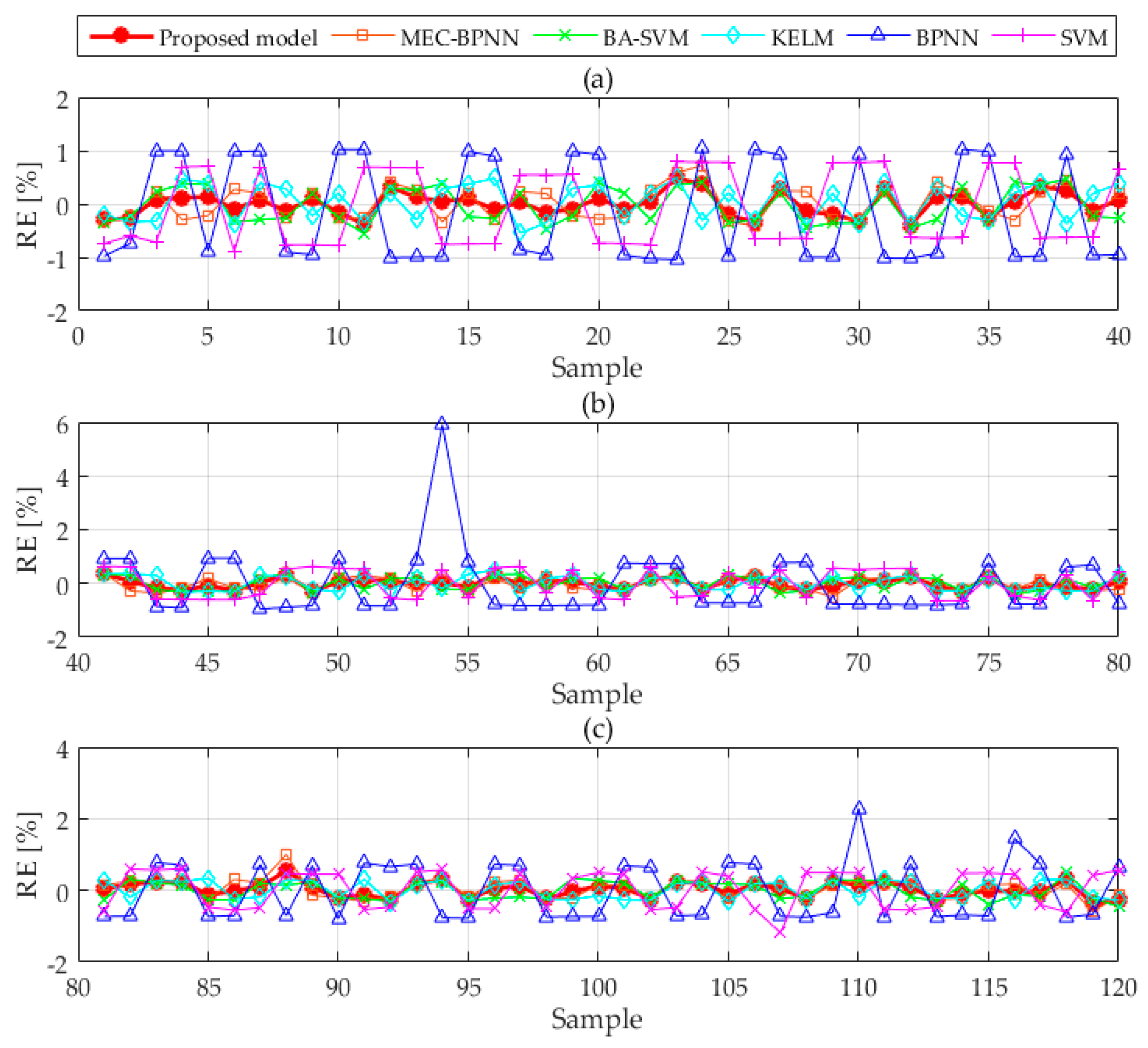
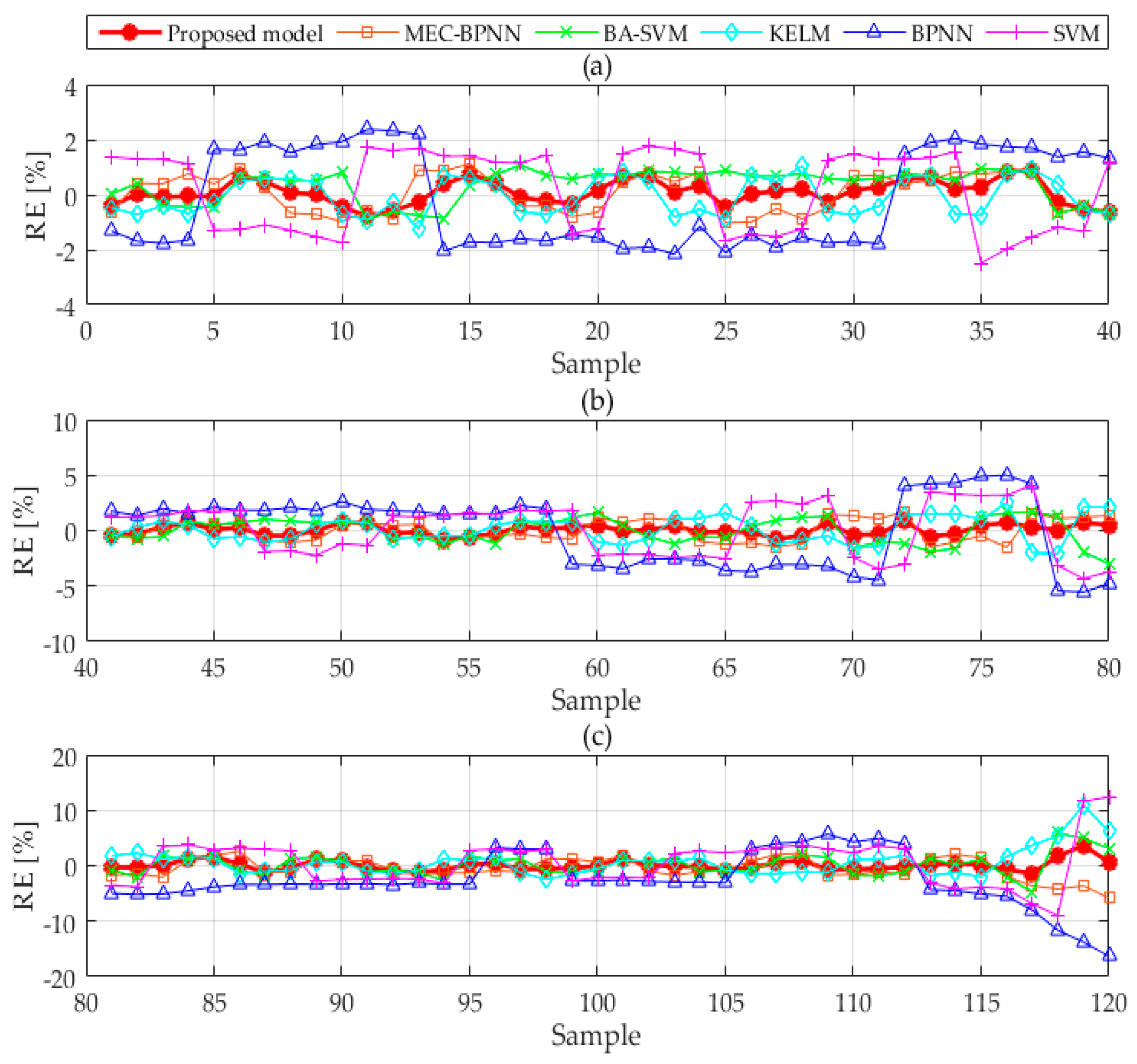
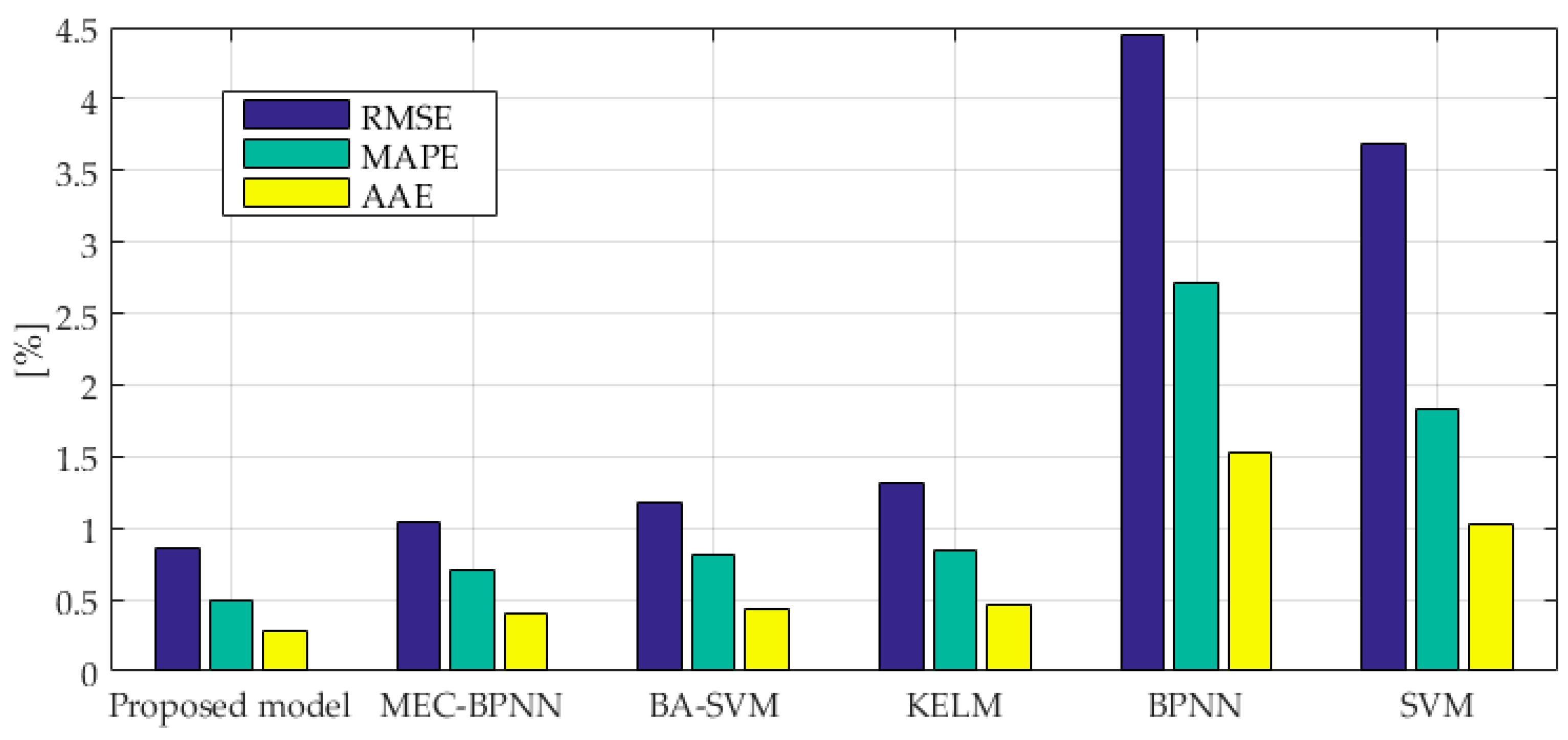
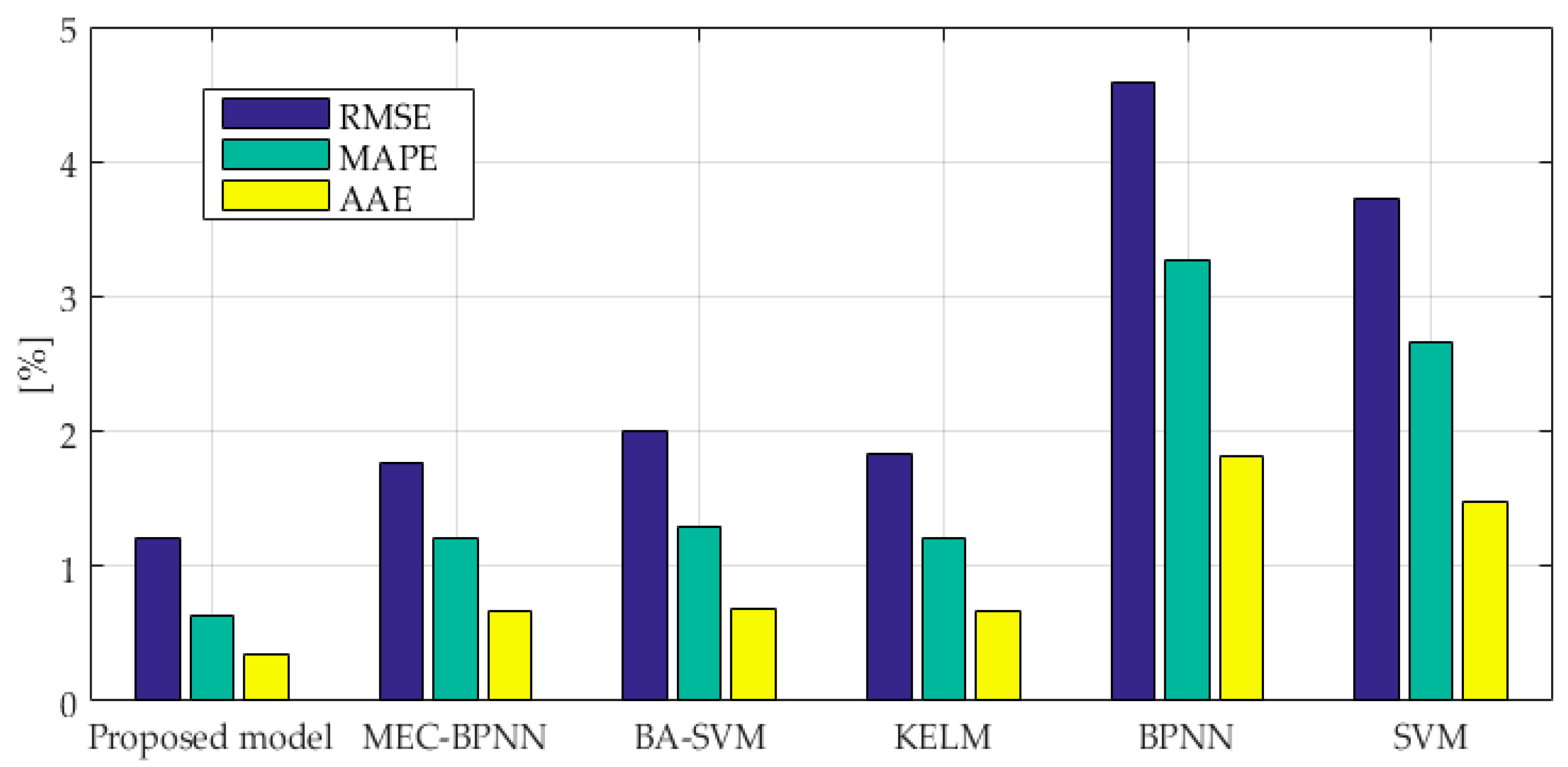
, are shown in Figure 4. The relative forecasting error of each model is revealed in Figure 5. This paper divides the test set samples into four groups to show the forecasting effect of each model owing to the large model quantities and sample points. Figure 4 and Figure 5 therefore consist of three sub-graphs, respectively. The RMSE, MAPE and AAE of models are demonstrated in Figure 6.

The deviation between the icing thickness forecasting value and the original value of BPNN and SVM is large by contrasting the results of the six forecasting methods in Figure 4. In addition, the curves of forecasting value and original value are suddenly far or suddenly near, indicating that the forecasting accuracy and robustness of these two methods are poor. Besides, the deviations of MEC-BPNN, BA-SVM and KELM are smaller than the above two models so that the precision is improved, but the curves are still like those with poor stability. However, the deviation which is obtained from improved BP-SVM-KELM based on VC is smaller and it is between the most accurate and the most inaccurate single improvement model. The value is the closest to the most precise model which indicates the accuracy of the combined forecasting model is guaranteed. Then the curves distance between the forecasting value and the actual value of the composite model is basically distributed near the actual value curve, indicating that the combination forecasting model has the strongest robustness.

Figure 5 compares the relative errors of the six forecasting methods. By counting the maximum and minimum relative errors, it can be found that the maximum relative errors of BPNN, SVM, MEC-BPNN, BA-SVM, KELM and the combined forecasting model are 5.910%, 1.186%, 1.003%, 0.551%, 0.545% and 0.543%, the minimum values are 0.611%, 0.170%, 0.135%, 0.119% and 0.002%. The maximum and minimum values in the three improved models are less than the two basic models, which shows that the prediction accuracy is better than the BPNN model and the SVM model. The maximum and minimum values in combined forecasting model are less than the three individual improved models, indicating that its prediction value is the nearest to optimal single improved model. The fluctuation ranges of the RE curves of the two basic models are the largest showing their stabilities are the poorest, and the stabilities of the three improved models have improved with a relatively small range of fluctuation. However, compared with the combination forecasting model, the fluctuation range is still large, which shows that the combination forecasting model plays a role in avoiding the weaknesses and improves the stability of prediction under the premise of ensuring the accuracy.

As we can see from Figure 6, the RMSE value of the combination forecasting model is 0.86%, and the RMSE values of the BPNN, SVM, MEC-BPNN, BA-SVM and KELM models are 4.44%, 3.68%, 1.04% and 1.32%, respectively. The proposed combination forecasting model has a lower error and a higher accuracy than the other models which makes the accuracy of single points be higher than the worst though the VC combined method solved the problem of dynamic weight distribution. The value is infinitely close to the most accurate single model at this point, so its stability and accuracy can be fully guaranteed. The prediction results of the three improved models are better than SVM and BPNN models indicating that their prediction performance has been improved by intelligent algorithms. The MAPE values of the BPNN, SVM, MEC-BPNN, BA-SVM, KELM and the combination forecasting models are 2.71%, 1.83%, 0.70%, 0.81%,0.84% and 0.50%. The evaluation index also shows that the combination forecasting method has the best overall prediction effect, the three improved models are second, and the two basic models have the worst prediction performance. The AAE value of the combination forecasting method is the smallest which enough shows the overall prediction performance of the proposed model is the best.

In conclusion, the prediction accuracy of the three improved models is advanced through the improvement of the basic model, but the robustness is still poor. The combination prediction model is not the most accurate at each point, but it is the closest to the most accurate predictions because the weights tend to the model with the highest accuracy according to the weight distribution. In the unknown prediction, the combination method can make best use of the advantages and bypass the disadvantages, so the flexibility, adaptability and accuracy are guaranteed.

4. Further Simulation

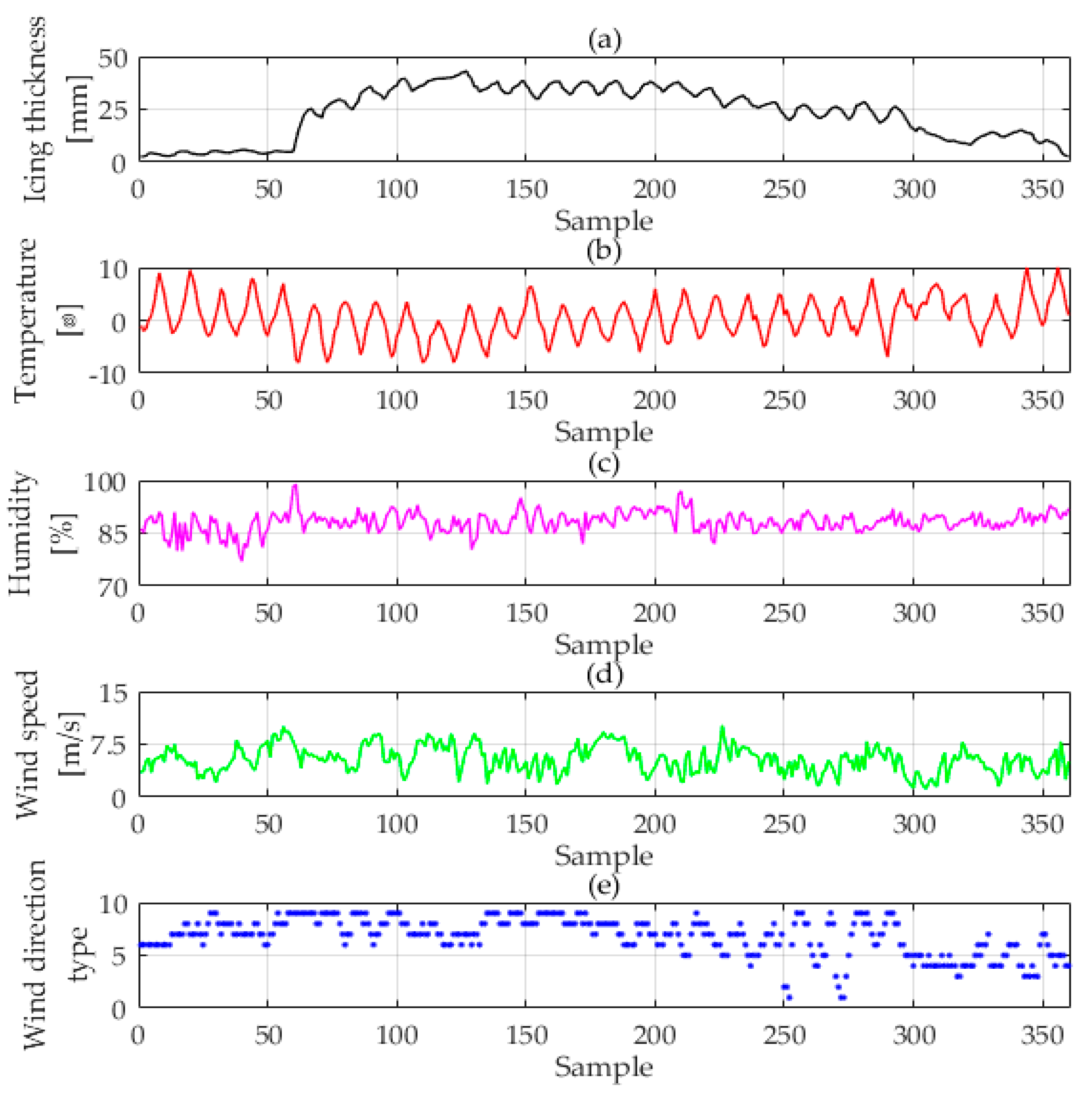
This paper now selects another line in Hunan, the "Tianshang line", as a case to further verify the performance of the proposed model. The data of “Tianshang line” are from 17 January 2008 to 15 February 2008, and have a total of 360 data groups. The first 240 are training samples and the latter 120 are test samples. All data of icing thickness, temperature, humidity, wind speed and wind direction clustering are shown in Figure 7. Like Case 1, all of the data were provided by the Key Laboratory of Disaster Prevention and Mitigation of Power Transmission and Transformation Equipment (Changsha, China), where all the data are collected by professional instruments and can reflect the state changes in the icing process. As we can see from Figure 7, the temperature data first decreases periodically, then rises periodically. The data of relative air humidity and wind speed present a cyclical upward trend. What’s more, there is no exception data or missing data. Hence these data can be used directly as data sources.

BPNN, SVM, MEC-BPNN, BA-SVM, KELM and thw improved BP-SVM-KELM combination model based on VC are utilized to compare and analyze in this section. The parameter setting of BPNN, MEC-BPNN, and KELM are consistent with the previous case. In the single SVM model, the penalty parameter c is 10.307, the kernel function parameter g is 0.328, and the ε loss function parameter p is 2.261. For the same case, the SVM optimal penalty parameter c is 2.083, the kernel parameter g is 0.012 and the ε loss function parameter p is 0.011 by BA optimization. The combination weights of the three individual models of MEC-BPNN, BA-SVM and KELM are 0.40, 0.25 and 0.35, respectively, through the VC combined method that solved the problem of dynamic weight distribution.

The results of the k-fold cross validation for the three modified models proposed in this paper are described in

Table 4. Results of the k-fold cross validation.

Fold Number	RMSE of MEC-BPNN	RMSE of BA-SVM	RMSE of KELM
1	0.0178	0.0217	0.0182
2	0.0156	0.0233	0.0181
3	0.0182	0.0202	0.0192
4	0.0166	0.0193	0.0169
5	0.0167	0.0205	0.0175
6	0.0198	0.0202	0.0196
7	0.0202	0.0192	0.0185
8	0.0186	0.0178	0.0179
9	0.0191	0.0191	0.0192
10	0.0182	0.0203	0.0197
11	0.0175	0.0195	0.0186
12	0.0190	0.0212	0.0192
Average Value	0.0181	0.0202	0.0186
Standard Deviation	0.00130	0.00136	0.00083

. A part of the forecasting values and relative errors of each model is listed in

Table 5. Part of the forecasting value and relative errors of each model.

Data Point Number	Actual Value (mm)	BPNN		SVM		MEC-BPNN		BA-SVM		KELM		Proposed Model
		Forecast Value	Error %	Forecast Value	Error %	Forecast Value	Error %	Forecast Value	Error %	Forecast Value	Error %	Forecast Value	Error %
1	26.38	26.729	−1.32	26.02	1.36	26.54	−0.61	26.37	0.04	26.51	−0.49	26.49	−0.40
2	26.97	27.426	−1.69	26.62	1.30	26.86	0.41	26.86	0.41	27.16	−0.70	26.96	0.02
3	27.32	27.801	−1.76	26.969	1.28	27.21	0.40	27.432	−0.41	27.43	−0.40	27.34	−0.09
4	27.68	28.136	−1.65	27.37	1.12	27.47	0.76	27.8	−0.43	27.87	−0.69	27.69	−0.05
5	28.01	27.55	1.64	28.37	−1.29	27.9	0.39	28.14	−0.46	28.09	−0.29	28.03	−0.06
6	28.32	27.86	1.62	28.68	−1.27	28.05	0.95	28.14	0.64	28.18	0.49	28.12	0.71
7	27.87	27.33	1.94	28.176	−1.10	27.8	0.25	27.69	0.65	27.71	0.57	27.74	0.46
8	25.51	25.12	1.53	25.84	−1.29	25.68	−0.67	25.38	0.51	25.36	0.59	25.49	0.07
9	23.65	23.22	1.82	24.01	−1.52	23.82	−0.72	23.53	0.51	23.54	0.47	23.65	0.01
10	22.35	21.92	1.92	22.74	−1.74	22.57	−0.98	22.17	0.81	22.51	−0.72	22.45	−0.43

. The forecasting results of each model are described in Figure 8, and the relative errors are shown in Figure 9. The RMSE, MAPE and AAE are shown in Figure 10.

As is shown in Table 4, the average RMSE values of MEC-BPNN, BA-SVM and KELM are 0.0181, 0.0202 and 0.0186, respectively. In addition, the RMSE standard deviations of MEC-BPNN, BA-SVM and KELM are 0.00130, 0.00136 and 0.00083, respectively. These data illustrate the fact again that the generalization performance of the three modified models has been improved.

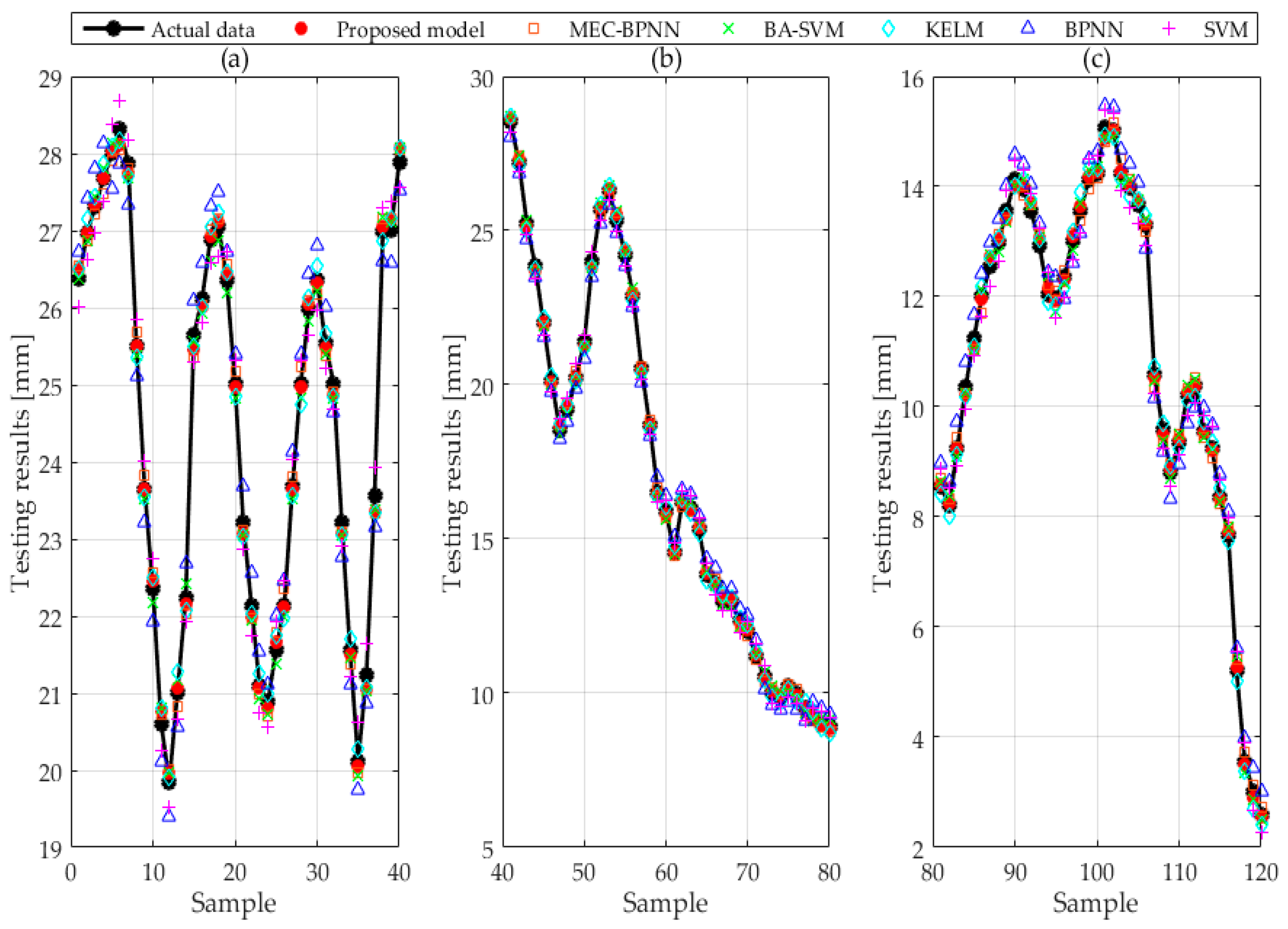
As we see from Figure 8 and Table 5, compared with the BPNN and SVM models, the forecasting values of the three improved models are closer to the original values, which shows that the prediction accuracy of the modified model is better. The forecasting value of combination model is between the forecasting values of the three modified models. Although the proposed model is not the most accurate, the change range of the distance between the prediction and the actual value curves is the smallest. Besides, the result of the combination forecast model is closer to the most accurate single model predictive value which further shows that the combination forecasting model greatly improves the stability of prediction under the premise of ensuring accurate prediction.

The relative errors of the BPNN model and the SVM model are at a high level and the fluctuation range is large by observing Figure 9, where the relative forecasting error of the six models are displayed, indicating that the two models’ accuracy and robustness are poor. As we can see from Figure 9 and Table 5, the relative errors of MEC-BPNN, BA-SVM and KELM are lower than those of the two basic models with greater volatility, and the value at some points is still large, which shows that its accuracy has been improved while the stability is still not guaranteed. It can be found that the relative errors of the three modified models constantly change their ranking at various points, which can be classified into three cases. For instance, in the first case, the relative errors of MEC-BPNN, BA-SVM and KELM are 1.13%, 1.64% and −1.01%, respectively, at the 60th sample point, where the forecasting accuracy of KELM is the highest. In the second case, the relative errors of MEC-BPNN, BA-SVM and KELM are 1.35%, −3.04% and 2.14%, respectively, at the 80th sample point, where the forecasting accuracy of MEC-BPNN is the highest. In the third case, the relative errors of MEC-BPNN, BA-SVM and KELM are −5.81%, 3.10% and 6.20%, respectively, at the 120th sample point, where the forecasting accuracy of BA-SVM is the highest. However, the relative error curve of the proposed combination model is among the three curves of MEC-BPNN, BA-SVM and KELM and it is close to the most accurate prediction in almost every sample point. In addition, its fluctuation range is also narrower. This indicates that the combination model can obtain both accurate and stable forecasting results.

As is shown in Figure 10, the RMSE, MAPE and AAE of the proposed combination forecasting model are the minimum at 1.20%, 0.63% and 0.34%. This indicates that its whole predictive performance is optimal. By observing these values of the three improved model, it can be found that the whole prediction accuracy of MEC-BPNN is better than KELM’s, and KELM’s is superior to BA-SVM’s. When adopting the VC combined method to solve the problem of dynamic weight distribution to assign weights, MEC-BPNN’s weight is the highest, KELM’s is the second and BA-SVM’s is the minimum. It shows that weight assignation of the proposed combination forecasting method leans toward the most precise model, which enhances the robustness of prediction and also guarantees the accuracy.

By comparing the case with the previous one, it is clear that the weights of the three individual improvement models differ from those of the previous case. The prediction accuracy of BA-SVM is better than that of KELM and its weight is higher than KELM’s in the Case 1 according to the calculation results of performance evaluation index. However, the Case 2 is just the opposite. The difference indicates that the VC combined method solved the problem of dynamic weight distribution can adjust the weights according to the prediction accuracy of each individual model. It is so flexible that the overall accuracy of the prediction is improved.

In summary, the paper introduces the MEC-BP model, the BA-SVM model and the KELM model to improve the prediction performance of the individual models. The VC combined method solved the problem of dynamic weight distribution combines these models’ advantages, and the weights are flexibly assigned, so the overall instability of the model is reduced and satisfactory prediction results are obtained.

5. Conclusions

In order to obtain better accuracy and stability of icing forecasting, an innovative combination forecasting model using a modified Back Propagation Neural Network-Support Vector Machine-Extreme Learning Machine with Kernel (BPNN-SVM-KELM) based on the variance-covariance (VC) weight determination method is proposed in this paper. First of all, BPNN is optimized by a mind evolutionary algorithm (MEC) to solve the problem that BPNN often falls into local optima and converges slowly. Second, a bat algorithm (BA) is used to optimize SVM, and the problem of choosing SVM key parameters is solved. Third, the kernel function is introduced into ELM to improve the regression forecasting accuracy of the model. Finally, by the dynamic allocation method of VC weights, three improved models of MEC-BPNN, BA-SVM and KELM are combined to obtain the combination forecasting model. In the simulation process, this paper takes into account the strong fluctuation of wind direction data, which will have a negative impact on the accuracy of forecasting. Therefore, according to the influence degree of wind direction on icing thickness, a clustering processing is carried out. Through the simulation of two examples, it is clear that three individual modified models utilize various optimization algorithms to take advantage of the core advantages of the forecasting model, avoiding the defects of the model itself and optimizing the performance of the model. Furthermore, the VC weighted combination method is used to dynamically assign weights, and the forecasting results tend to the best single prediction model. It is proved that the combination method complements the shortcomings of each model and has a strong comprehensive response ability. In summary, the research content of this paper is expected to provide a useful reference for the power sector to deal with icing accidents in advance.

References

1. Jiang, X.; Xiang, Z.; Zhang, Z.; Hu, J. Predictive model for equivalent ice thickness load on overhead transmission lines based on measured insulator string deviations. IEEE Trans. Power Deliv. 2014, 29, 1659–1665. [Google Scholar] [CrossRef]
2. Chang, S.E.; Mcdaniels, T.L.; Mikawoz, J.; Peterson, K. Infrastructure failure interdependencies in extreme events: power outage consequences in the 1998 ice storm. Nat. Hazards 2007, 41, 337–358. [Google Scholar] [CrossRef]
3. Hou, H.; Yin, X.; You, D.; Chen, Q.; Tong, G.; Zheng, Y.; Shao, D. Analysis of the Defects of Power Equipment in the 2008 Snow Disaster in Southern China Area. High Volt. Eng. 2009, 35, 584–590. [Google Scholar]
4. Lü, Y.; Zhan, Z.; Ma, W. Design and application of online monitoring system for ice-coating on transmission lines. Power Syst. Technol. 2010, 34, 196–200. [Google Scholar]
5. Wang, H.L.; Shi-Ming, Y.U.; Fan, Y.M. Transmission line icing monitoring system based on wireless sensor net works. Manuf. Autom. 2011, 17, 150–153. [Google Scholar]
6. Luo, J.; Li, L.; Ye, Q.; Hao, Y.; Li, L. Development of Optical Fiber Sensors Based on Brillouin Scattering and FBG for On-Line Monitoring in Overhead Transmission Lines. J. Lightwave Technol. 2013, 31, 1559–1565. [Google Scholar] [CrossRef]
7. Imai, I. Studies on ice accretion. Res. Snow Ice 1953, 3, 35–44. [Google Scholar]
8. Goodwin, E.J.I.; Mozer, J.D.; Digioia, A.M.J.; Power, B.A. Predicting Ice and Snow Loads for Transmission. Available online: http://www.dtic.mil/docs/citations/ADP001696 (accessed on 11 August 2017).
9. Lenhard, R.W. An indirect method for estimating the weight of glaze on wires. Bull. Am. Meteorol. Soc. 1995, 36, 1–5. [Google Scholar]
10. Zhang, Z.; Huang, H.; Jiang, X.; Hu, J.; Sun, C. Analysis of Ice Growth on Different Type Insulators Based on Fluid Dynamics. Trans. China Electrotech. Soc. 2012, 27, 35–43. [Google Scholar]
11. Li, P.; Zhao, N.; Zhou, D.; Cao, M.; Li, J.; Shi, X. Multivariable time series prediction for the icing process on overhead power transmission line. Sci. World J. 2014, 2014, 1–9. [Google Scholar] [CrossRef] [PubMed]
12. Yang, J.L. Impact on the Extreme Value of Ice Thickness of Conductors from Probability Distribution Models. In Proceedings of the International Conference on Mechanical Engineering and Control Systems, IEEE Computer Society, Washington, DC, USA, 23–25 January 2015. [Google Scholar]
13. Li, P.; Li, Q.; Cao, M.; Gao, S.; Huang, H. Time Series Prediction for Icing Process of Overhead Power Transmission Line Based on BP Neural Networks. In Proceedings of the 2011 30th Chinese Control Conference (CCC), Yantai, China, 22–24 July 2011. [Google Scholar]
14. Wang, L.; Luo, Y.; Yao, Y. Analysis of transmission line icing detection and prediction based on neural network. J. Chongqing Univ. Posts Telecommun. 2012, 24, 254–258. [Google Scholar]
15. Zheng, Z.; Liu, J. Prediction method of ice thickness on transmission lines based on the combination of GA and BP neural network. Power Syst. Clean Energy 2014, 30, 27–30. [Google Scholar]
16. Wang, J.W. Ice thickness prediction model of transmission line based on improved particle swarm algorithm to optimize nrbf neural network. J. Electr. Power Sci. Technol. 2012, 27, 76–80. [Google Scholar]
17. Zarnani, A.; Musilek, P.; Shi, X.; Ke, X.; He, H.; Greiner, R. Learning to predict ice accretion on electric power lines. Eng. Appl. Artif. Intell. 2012, 25, 609–617. [Google Scholar] [CrossRef]
18. Huang, J.; Yang, H.; Hunan, Y.W. Forecast of line ice-coating degree using circumfluence index & support vector machine method. In Proceedings of the International Conference on Electric Utility Deregulation and Restructuring and Power Technologies, Changsha, China, 26–29 November 2015. [Google Scholar]
19. Xu, X.; Niu, D.; Wang, P.; Lu, Y.; Xia, H. The weighted support vector machine based on hybrid swarm intelligence optimization for icing prediction of transmission line. Math. Probl. Eng. 2015, 2015, 1–9. [Google Scholar] [CrossRef]
20. Ma, T.; Niu, D. Icing Forecasting of High Voltage Transmission Line Using Weighted Least Square Support Vector Machine with Fireworks Algorithm for Feature Selection. Appl. Sci. 2016, 6, 438. [Google Scholar] [CrossRef]
21. Ma, T.; Niu, D.; Fu, M. Icing forecasting for power transmission lines based on a wavelet support vector machine optimized by a quantum fireworks algorithm. Appl. Sci. 2016, 6, 54. [Google Scholar] [CrossRef]
22. Jie, J.; Zeng, J.; Han, C. An extended mind evolutionary computation model for optimizations. Appl. Math. Comput. 2007, 185, 1038–1049. [Google Scholar] [CrossRef]
23. Yang, X.S. A new metaheuristic bat-inspired algorithm. Comput. Knowl. Technol. 2010, 284, 65–74. [Google Scholar]
24. Liu, N.; Zhang, Q.; Liu, H. Online Short-Term Load Forecasting Based on ELM with Kernel Algorithm in Micro-Grid Environment. Trans. China Electrotech. Soc. 2015, 30, 218–224. [Google Scholar]
25. Wang, D.; Wei, S.; Luo, H.; Yue, C.; Grunder, O. A novel hybrid model for air quality index forecasting based on two-phase decomposition technique and modified extreme learning machine. Sci. Total Environ. 2017, 580, 719–733. [Google Scholar] [CrossRef] [PubMed]
26. Jiang, Y.; Liu, Z.; Luo, H.; Wang, H. Elm indirect prediction method for the remaining life of lithium-ion battery. J. Electr. Meas. Instrum. 2016, 30, 179–185. [Google Scholar]
27. Huang, G.B.; Zhu, Q.Y.; Siew, C.K. Extreme learning machine: Theory and applications. Neurocomputing 2006, 70, 489–501. [Google Scholar] [CrossRef]
28. Bates, J.M.; Granger, C.W.J. Combination of forecasts. Oper. Res. Quart. 1969, 20, 451–468. [Google Scholar] [CrossRef]
29. Liang, Y.; Niu, D.; Cao, Y.; Hong, W.C. Analysis and modeling for china’s electricity demand forecasting using a hybrid method based on multiple regression and extreme learning machine: A view from carbon emission. Energies 2016, 9, 941. [Google Scholar] [CrossRef]
30. Wang, J.; Hu, J. A robust combination approach for short-term wind speed forecasting and analysis—combination of the arima, elm, svm and lssvm forecasts using a gpr model. Energy 2015, 93, 41–56. [Google Scholar] [CrossRef]
31. Hui-Lin, L. Applications of the combination weighted arithmetic averaging operator in the delivery merchandise sale forecast of material resources. J. Nat. Sci. Heilongjiang Univ. 2012, 29, 22–28. [Google Scholar]
32. Han, W.; Wang, J.; Zhang, X.H. Application Research of Combined Forecasting Based on Induced Ordered Weighted Averaging Operator. Manag. Sci. Eng. 2014, 8, 23–26. [Google Scholar]
33. Zhang, H.; Zhu, Y.J.; Fan, L.L.; Qiao-Ling, W.U. Mid-long term load interval forecasting based on markov modification. East China Electr. Power 2013, 41, 33–36. [Google Scholar]
34. Xian, G.M. ε-svr algorithm and its application. Comput. Eng. Appl. 2008, 44, 40–42. [Google Scholar]
35. Kohavi, R. A study of cross-validation and bootstrap for accuracy estimation and model selection. In Proceedings of the 14th International Joint Conference on Artificial Intelligence, Montreal, QC, Canada, 20–25 August 1995. [Google Scholar]
36. Huang, G.B.; Wang, D. H.; Lan, Y. Extreme learning machines: a survey. Int. J. Mach. Learn. Cybern. 2011, 2, 107–122. [Google Scholar] [CrossRef]
37. Huang, G.B.; Zhou, H.; Ding, X.; Zhang, R. Extreme learning machine for regression and multiclass classification. IEEE Trans. Syst. Man Cybern. Part B Cybern. 2012, 42, 513–529. [Google Scholar] [CrossRef] [PubMed]
38. Huang, X.B.; Ouyang, L.S.; Wang, Y.N.; Li-Cheng, L.I.; Bing, L. Analysis on key influence factor of transmission line icing. High Volt. Eng. 2011, 37, 1677–1682. [Google Scholar]
Figure 1. Combination forecasting model.
Energies 10 01196 g001
Figure 2. Original data chart of icing thickness, temperature, humidity, wind speed, and wind direction. Note: (a) represents the original data of icing thickness; (b) represents the original data of temperature; (c) represents the original data of humidity; (d) represents the original data of wind speed; (e) represents the original data of wind direction.
Energies 10 01196 g002
Figure 3. The wind direction processing data of "Dong-Chao line".
Energies 10 01196 g003
Figure 4. The forecasting values of different methods: (a) the forecasting value from 1 to 40 sample point; (b) the forecasting value from 41 to 80 sample point; (c) the forecasting value from 81 to 120 sample point.
Energies 10 01196 g004
Figure 5. The relative errors curve of each method: (a) the relative error from 1 to 40 sample point; (b) the relative error from 41 to 80 sample point; (c) the relative error from 81 to 120 sample point.
Energies 10 01196 g005
Figure 6. Values of root-mean-square error (RMSE), mean absolute percentage error (MAPE) and average absolute error (AAE).
Energies 10 01196 g006
Figure 7. Original data of icing thickness, temperature, humidity, wind speed, and the processing data of wind direction. Note: (a) represents the original data of icing thickness; (b) represents the original data of temperature; (c) represents the original data of humidity; (d) represents the original data of wind speed; (e) represents the processing data of wind direction.
Energies 10 01196 g007
Figure 8. The forecasting values of different methods: (a) the forecasting value from 1 to 40 sample point; (b) the forecasting value from 41 to 80 sample point; (c) the forecasting value from 81 to 120 sample point.
Energies 10 01196 g008
Figure 9. The relative errors curve of each method: (a) the relative error from 1 to 40 sample point; (b) the relative error from 41 to 80 sample point; (c) the relative error from 81 to 120 sample point.
Energies 10 01196 g009
Figure 10. Values of root-mean-square error (RMSE), mean absolute percentage error (MAPE) and average absolute error (AAE).
Energies 10 01196 g010