Switched Control Strategies of Aggregated Commercial HVAC Systems for Demand Response in Smart Grids


1
School of Electrical Engineering, Yanshan University, Qinhuangdao 066004, China
2
Key Laboratory of System Control and Information Processing, Ministry of Education, Shanghai Jiao Tong University, Shanghai, 200240, China
*
Author to whom correspondence should be addressed.
Energies 2017, 10(7), 953; https://doi.org/10.3390/en10070953
Submission received: 17 April 2017
/
Revised: 29 June 2017
/
Accepted: 4 July 2017
/
Published: 9 July 2017
(This article belongs to the Special Issue Energy Management Control)
Abstract
:This work proposes three switched control strategies for aggregated heating, ventilation, and air conditioning (HVAC) systems in commercial buildings to track the automatic generation control (AGC) signal in smart grid. The existing control strategies include the direct load control strategy and the setpoint regulation strategy. The direct load control strategy cannot track the AGC signal when the state of charge (SOC) of the aggregated thermostatically controlled loads (TCLs) exceeds their regulation capacity, while the setpoint regulation strategy provides flexible regulation capacity, but causes larger tracking errors. To improve the tracking performance, we took the advantages of the two control modes and developed three switched control strategies. The control strategies switch between the direct load control mode and the setpoint regulation mode according to different switching indices. Specifically, we design a discrete-time controller and optimize the controller parameter for the setpoint regulation strategy using the Fibonacci optimization algorithm, enabling us to propose two switched control strategies across multiple time steps. Furthermore, we extend the switched control strategies by introducing a two-stage regulation in a single time step. Simulation results demonstrate that the proposed switched control strategies can reduce the tracking errors for frequency regulation.
1. Introduction
As smart grid construction is rapidly executed and large-scale intermittent renewable energy resources are being integrated, demand response programs enable consumers to schedule loads in order to save energy, reduce costs, and help grid operation [1]. Ancillary service, which is required to support the reliable delivery of electricity and the operation of transmission systems, is an important component of electric service. Ancillary service includes voltage control, black start, spinning reserve, replacement, load following, and frequency regulation [2].
In the power grid, the imbalance between the generation and the load often results in mismatches in frequency [3]. Traditionally, rapidly responding generators and grid-scale energy storage units have provided frequency regulation [4]. Since the schedulable electrical loads are popular in commercial buildings and residences, they have become promising candidates in enhancing the property of power systems. As the main components of schedulable electrical loads, thermostatically-controlled loads (TCLs), which include heat pumps, chillers, and air conditioners, are suitable for regulating their aggregate power to serve for the demand response [5,6,7,8]. A simple TCL, such as a frequency-fixed air conditioner, usually has two operation states, i.e., on/off, each of which corresponds to one output power level, or 0. The simple on/off state transition makes it possible for the TCLs to participate in ancillary service. When the generation is in surplus, the TCLs can “charge” by turning on, and during the periods of scarcity, they “discharge” by turning off [9]. The dynamic modeling of TCLs was first studied in [10] and applied in cold load pickup. A variation of the alternating direction method of multipliers (ADMM) algorithm was proposed to achieve the distributed optimization of aggregated TCLs [11].
As a representative type of TCLs, the heating, ventilation, and air conditioning (HVAC) units, which are widely installed in commercial buildings, are studied and analyzed widely in terms of different aspects. It is essential to study the load dynamics, the model parameters, the temperature evolution, and the power consumption of HVAC units. The control of the air pressure and temperature for HVAC units was considered to keep rooms in desired conditions by the authors of [12,13,14]. The energy management of HVAC units was developed to remove the peak load and match supply with demand by the authors of [15,16,17].
The HVAC units are usually regulated by turning them on or off directly. A state queuing model and a temperature priority list strategy were presented in [18] to control the on/off states of the HVAC units. A centralized control framework of the HVAC units was presented in [19,20,21] to provide continuous regulation services, and the operational characteristics were analyzed under different system states and communication models. A novel two-level scheduling method was proposed in [22] to minimize the energy imbalance cost. In [23], the authors modeled the aggregated HVAC units as a generalized energy storage battery and proposed a temperature-priority control strategy to control the power consumption to track the frequency regulation signal to serve for the grid, and the tracking errors were reduced by controlling the on/off states directly. The temperature setpoint and the deadband are not regulated in this control mode, which limits the HVAC units’ ability to “store” or “release” energy. Furthermore, the tracking error is extremely large when the synchronization of loads occurs.
Setpoint regulation is another control strategy to regulate the HVAC units [24]. The authors of [25,26,27,28] proposed several types of controllers, such as the internal model controller, the linear quadratic controller and the Lyapunov stable controller to achieve peak shaving or load shifting by regulating the temperature setpoint. A heuristic algorithm based on the setpoint regulation was developed for decentralized implementation in [29]. Regulating the temperature setpoint enlarges the energy storage capacity, but the setpoint regulation causes large chattering effects and tracking errors.
To reduce the errors when tracking the automatic generation control (AGC) signal, we combine the two types of control strategies and develop three switched control strategies. Specifically, the direct load control strategy is used when the energy capacity is sufficient, and the setpoint regulation strategy is adopted when the capacity is insufficient. To implement the switching control strategies, we must first address two problems: What is the optimal control law for temperature setpoint regulation? What is the best method for switching between the two control strategies? This study deals with these problems and achieves the following contributions:
- A discrete-time controller is proposed to adjust the setpoints of the HVAC units and the Fibonacci optimization algorithm is used in [30] to obtain the optimal parameter of the controller.
- The switching indices are established before presenting the switched control strategies to track the AGC signal.
- A two-stage regulation strategy is proposed in a single time step to improve the tracking performance of the switched control strategies.
The rest of the paper is organized as follows. Section 2 describes the operation characteristics of the HVAC units and the two typical control strategies, and then establishes the switched control model. Section 3 covers the controller design and parameter optimization using the Fibonacci algorithm and presents three switched control strategies across multiple time steps. The simulation results are shown in Section 4 , and the conclusions are summarized in Section 5 .
2. System Model and Control Strategies
This section introduces the individual HVAC model and the typical control strategies in commercial buildings before establishing a switched control model.
2.1. Individual HVAC Model
The coupled equivalent thermal parameters (ETP) model includes two temperature variables, the internal air temperature T and the mass temperature [31], while the simplified HVAC model only contains T under the assumption that is equal to T [19,20,21]. In this work, we use the simplified HVAC model [32]. For a system including N HVAC units, the temperature evolution of the i-th HVAC unit in the cooling mode can be expressed as:
where,
and is a binary variable, which represents whether the HVAC unit is on or off. The power consumption of the aggregated HVAC units can be calculated by:
2.2. Typical Control Strategies
The typical control strategies of the aggregated HVAC units in commercial buildings can be classified into two categories: the direct load control strategy and the setpoint regulation strategy. The specific control processes are described below.
The first type of control strategies is based upon the on/off state control, namely the direct load control. According to the state information, the control center decides which loads should be turned on or off based on certain strategies, such as the temperature priority control strategy [23]. Specifically, the internal air temperatures order the aggregated loads. The “on” loads with lower indoor temperatures have a higher priority to turn off, and the “off” loads with higher indoor temperatures have a higher priority to turn on in the cooling mode. Then the loads will be turned on or off in sequence until the desired objective is achieved, and the on/off operations in sequence can make full use of the reserve capacity of the HVAC units. It was suggested that the direct load control strategy is restricted by the state of charge (SOC) of the aggregated loads [23]. When the SOC exceeds the capacity limits, the aggregated loads cannot track the AGC signal anymore.
The second type of control strategies is based on setpoint regulation. For instance, a bilinear system model was derived in [33] to approximate the dynamics of the aggregate HVACs, and a sliding-mode control strategy in the continuous-time form was developed to regulate the setpoint. It was concluded that the aggregated loads cannot track the AGC signal when the stability condition is not satisfied [33].
2.3. Control Strategy Comparison
The main difference between the two control strategies is the temperature range of the loads to be scheduled. One is to control all the loads directly in the whole deadband, except for the loads which must be on or off due to the temperature limits. The other is to regulate the loads near the edges indirectly by their self-operations. The tracking performance is better under the temperature priority control strategy when the energy capacity is enough. The loads are only turned on or off with one more or less load than the control objective under the temperature priority control strategy. Although the energy capacity is enlarged dynamically by adjusting the setpoint in the sliding-mode control strategy, it will cause a larger tracking error.
We use a Monte Carlo method and MATLAB R2009a (MathWorks, Natick, MA, USA) to evaluate the performances of 1000 HVAC units under the two control strategies and give the simulation parameters in Table 1 [9,34], where R, C, and P are assumed to follow Gaussian distributions. These parameters can be obtained based on the methods in [35,36], e.g., the short-term energy monitoring (STEM) method. The averages of R, C, and P are shown in Table 1, and the standard deviations are 0.1. The initial load temperatures are assumed to be distributed uniformly in the deadband. The baseline power is set as:
The AGC signal within two hours is randomly chosen from the Pennsylvania–New Jersey–Maryland Interconnection (PJM) electricity markets to demonstrate the tracking performance [37]. The power deviation is defined as the difference between the aggregated power and the baseline power. The tracking performances during 2 h are shown in Figure 1 and Figure 2. The figure with 1000 HVAC units contains a lot of data and occupies large storage space. Without loss of generality, we randomly choose 100 out of them.
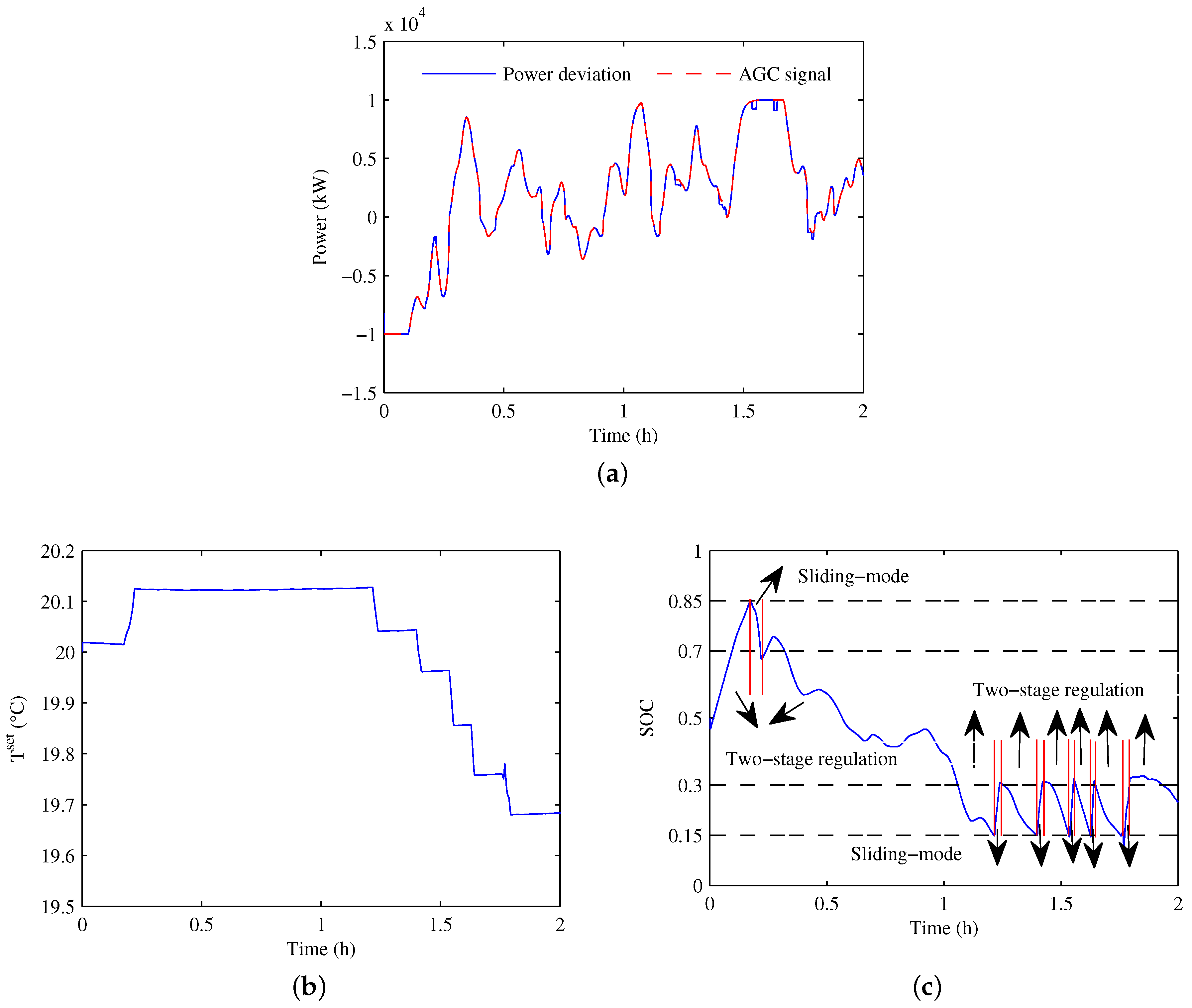
As shown in Figure 1, the tracking performance is good when the stored energy is still in the capacity bounds. However, when the loads are centered at the temperature edges, the synchronization occurs and the loads cannot track the signal. At the same time, the AGC signal exceeds the energy capacity so that the loads cannot track the regulation signal. It can be concluded that the centering at the temperature limits of HVAC units corresponds to the situation that the available energy capacity is depleted. Due to the temperature limits, some of the HVAC units must be turned on or off, so there are not enough HVAC units to be scheduled. It means that the energy is fully discharged or charged. In that case, the loads are turned on or off frequently, and the wear of the HVAC units is severe.
In Figure 2, the tracking error is caused by the chattering effects and is much larger than that in Figure 1 when the loads are not centering at edges, but the temperature distribution of loads is almost uniform. The energy storage capacity is enlarged, and the aggregated HVAC units can charge or discharge sustainedly. Moreover, since the scheduled loads are near the temperature edges, the “short-cycling” problem is avoided and the wear of the HVAC units is reduced. However, the change of the setpoint reduces the thermal comfort of consumers and the satisfaction levels.
Remark 1.
Figure 1 and Figure 2 are given to show the tracing performances of the temperature priority control strategy and the sliding-mode control strategy, respectively. It can be observed that the AGC signal within 2 h is enough to show the chattering effects and the case that the AGC signal exceeds the energy capacity.
2.4. Switched Control Model
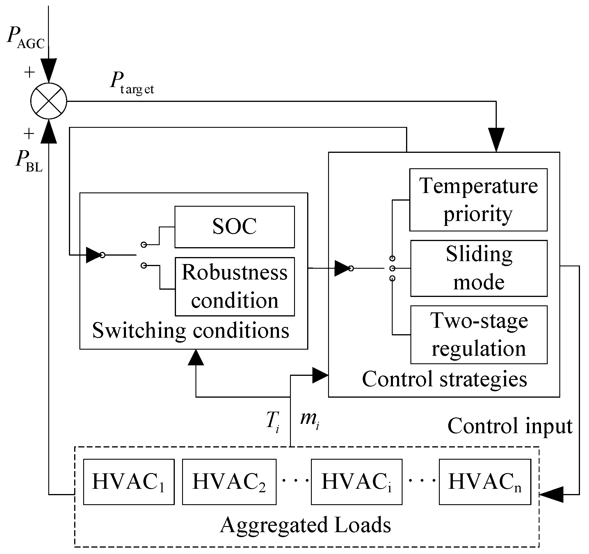
The switched control model is established based upon the two control strategies described in Section 2.2. The diagram of the switched control model across multiple time steps is shown in Figure 3.
The control center uses the SOC or the stability condition of the control gain as the switching indices and calculates them by collecting the state information of the HVAC units. Different control strategies are used to perform the tracking according to the values of the switching indices. The switched control strategies are achieved through the following steps:
- (1)
- First, we design a discrete-time sliding-mode controller to regulate the temperature setpoint and search for the optimal control gain by the Fibonacci optimization algorithm.
- (2)
- Second, we present a pair of switched control strategies according to two switching indices, which are then used to decide which control strategy should be applied across multiple time steps.
- (3)
- Third, we introduce a two-stage regulation in a single control cycle, which means that the loads are regulated twice in one time step. The third switched control strategy is then developed to further improve the tracking performance.
The specific description of the switched strategies is shown in Section 3 . We obtain the optimal parameter of the sliding-mode controller, design two switching indices, and consequently present three switched strategies.
3. Controller Design and Optimization
For a population of aggregated HVAC units, the average temperature deadband is divided uniformly into n bins, in which each bin contains the “on” loads and “off” loads. In that case, there are 2n states and any given HVAC unit corresponds to a certain state. The continuous-time model in [33] can be discretized into:
where is a 2n × 1 vector that represents the numbers of loads in each state, is the total power consumption, and is the average change of the temperature setpoint in the kth step. is a 1 × 2n vector, I is the identity matrix, and A is the state matrix:
The input matrix B is given by:
The parameters in A are detailed as,
The sliding-mode controller u in the discrete-time form is defined as,
where is the control gain, , and is the AGC power signal in time step k.
It was proven in [38] that the systems (7)–(8) are globally asymptotically stable with the sliding-mode controller (13) if satisfies a robustness condition:
where , , and . The robustness condition specifies the lower bound of the control gain. Due to the high frequency switching of the signum function, the chattering effect of the sliding mode controller is inevitable. It causes larger tracking errors and results in more meaningless state transitions of the HVAC units. To reduce the passive impact of the chattering effect on tracking performance, we applied the boundary layer-based method. This method is accomplished by substituting the signum function with a tunable saturation function, i.e.,
where , and is the width of boundary layer. The introduction of the boundary layer leads to the effective convergence of the tracking error to a zone bounded by . Therefore the final control input is:
When , the Lyapunov stability is not satisfied and the tracking error is large [33]. The state information ( and ) of the HVAC units should be measured in real time, and the parameters (, , and ) of the HVAC units should be collected to the controller. This depends on the advanced metering infrastructure (AMI) and the information processing capability of the control centers.
Remark 2.
In this control mode, the upper and lower temperature bounds are regulated along with the setpoints of the TCLs according to (4), and the deadband of each TCL is fixed.
3.1. Parameter Optimization
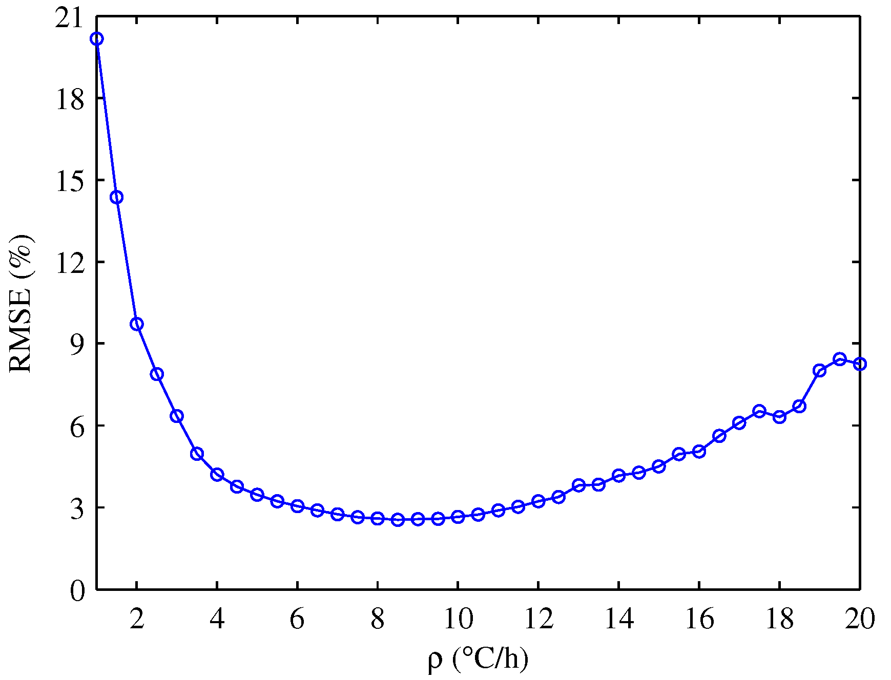
The tracking error in the setpoint regulation strategy is related to the control gain of the sliding-mode controller. It is necessary to find the optimal controller gain to improve the tracking performance. The root-mean-square error (RMSE) percentage is used to evaluate the tracking error, i.e., the deviation between the AGC signal and the actual response:
Adjusting the control gain according to the robustness condition in real time is a challenging work in practice because the AGC signal is highly unpredictable. In that case, is usually chosen large enough to satisfy (14). However, the large gain can induce the sliding-mode chattering effect, which results from the high frequency switching of the signum function. If is excessively large, the chattering effect is serious and the RMSE will increase significantly.
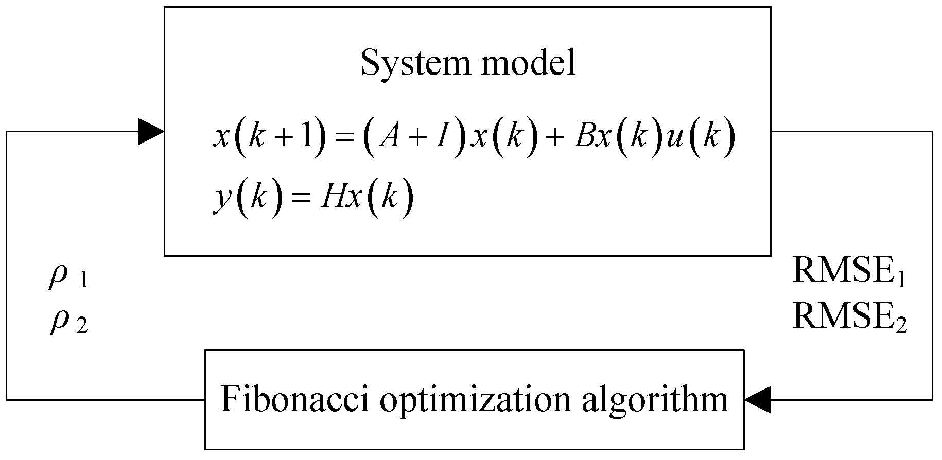
To find the relationship between RMSE and the gain , we calculated the actual RMSE values at different in Figure 4. From the figure, we can observe that the relationship between them is a unimodal function and there exists a minimum RMSE value. However, the exact analytic expression = is unknown. In that case, the analytical solution at the minimum RMSE cannot be obtained. However, the numerical solution can be achieved using the Fibonacci optimization Algorithm A1 [30]. The detailed description of it is shown in the Appendix A.
According to the diagram shown in Figure 5, C/h is calculated based on the historical statistical AGC data and can be used for future control. By utilizing the daily signals for 1 May through 10, 2014, we can observe that the optimal gains in different days are close across the time of day, as shown in Table 2. Thus, it is reasonable to take the mean value of them as the optimal gain. In this case, the mean value is 8.6 C/h, and it will be applied in the switched control strategies.
3.2. Switched Control Strategies I and II
In this subsection, two switched control strategies across multiple time steps are proposed to further reduce the tracking error. To achieve a smaller tracking error, we adopt different control strategies according to the operation states of the loads. It is necessary to define the switching indices and decide which control strategy should be applied.
For energy storage devices, an index named SOC is used to denote the state of charge; the index is the ratio of the remaining energy and rated capacity. The populations of HVAC units are represented as generalized battery models to analyze the aggregate flexibility. The SOC of the aggregated HVAC units under the cooling mode can be defined as:
If all room temperatures reach their upper limits, the SOC is 0, which means the stored energy is used up; if all room temperatures reach their lower limits, the SOC is 1, which means the stored energy is full. For traditional energy storage devices, the significant deep-discharging and over-charging process will reduce the service time. The same is true for the aggregated HVAC units because when the SOC is 1 or 0, the loads are centered at the edges and turn on or off frequently. We have noted that the loads are never centered at the edges in the setpoint regulation mode, which means that the deep-discharging or over-charging state can be avoided. Thus the SOC can be chosen as a switching index. The lower bound in (14) was selected as another switching index because when is not satisfied, the tracking error is large.
Four thresholds () of the SOC were introduced to establish the switched control strategies. The thresholds represent different energy states of the aggregated HVAC units. We can decide which control strategy should be applied according to whether the SOC reaches the thresholds and which thresholds the SOC reaches. The values of a and b represent that the SOC is close to the lower and upper energy limits, respectively. Once the SOC reaches a or b, the temperature priority control strategy should be switched to the sliding-mode control strategy. c and d represent that the SOC is far enough from the energy limits, and thus the temperature priority control strategy should be used.
3.3. Switched Control Strategy III
To further reduce the tracking error, we can utilize the precision tracking character of the temperature priority control and the ability of enlarging energy capacity of the sliding-mode control by adopting the two methods in a single time step. Figure 6 describes this basic idea. Assume that the loads are operating in the temperature region [, ] on the basis of the initial setpoint. In the first stage, the sliding-mode control strategy is used to increase or decrease the temperature setpoint, and the temperature region is changed to [, ]. After that, the loads are divided into an out-of-region group and an in-region group, namely Part 1 and Part 2. In the second stage, the temperature priority control strategy is used to control the loads in Part 2 to further reduce the tracking error.
This two-stage regulation in a time step is detailed as follows.
- Utilize the sliding-mode control strategy to track the AGC signal and output the tracking error.
- Divide the loads into Part 1 and Part 2.
- Control the loads in Part 2 based on the temperature-priority control strategy to compensate for the tracking error.
4. Simulation Results
In the simulation, we are referring to the theoretical HVAC systems described in Section 2. Here, HVAC units are used to track the daily AGC signal from the PJM electricity markets [37]. The simulation and control parameters are shown in Table 1. The initial upper and lower limits are calculated according to Equation (4), and the initial load temperatures are assumed to be distributed uniformly in the deadband. The switching thresholds were chosen based on the rule in Section 3.3. Their values are defined as , , , , and C/h. The power deviation is defined as the difference between aggregated power and baseline power.
The AGC tracking results, the temperature setpoint trajectories, and the SOC under the three switched control strategies are shown in Figure 8, Figure 9 and Figure 10, respectively.
From the temperature setpoint trajectories in Figure 8b and Figure 9b, it can be observed that the control modes were switched during the simulation. When the setpoint is not changed, the temperature priority mode is active, and otherwise, the sliding-mode strategy is active. Moreover, the switches can also be observed from the SOC results, i.e., Figure 8c and Figure 9c. Once one of the thresholds is reached, the control mode is changed correspondingly. However, the switches under Switched Control III can be only observed by the SOC results in Figure 10c because the temperature setpoint is regulated all the time in Figure 10b.
Furthermore, Table 4 provides comparisons of the RMSE, the variation range of the setpoint, and the number of on/off operations with the related works.
The large tracking error associated with the temperature priority control strategy was caused by the energy storage limits of the aggregated HAVC units. In fact, the tracking error is very small when the SOC does not exceed the energy storage limits [23]. The following observations were obtained from the simulation and comparison results:
- The tracking performances of the HVAC units under the three switched control strategies are better than they were when using the temperature priority control or the sliding-mode control individually. This is because that the switched control strategies select the appropriate control methods according to the system states. Hence, the disadvantage of each individual method is mitigated. It is observed that the switched control strategies have smaller RMSE and less stepoint changes, and thus they are promising for the frequency regulation.
- On the system operator side, the RMSE value is an important factor. A large RMSE means more reserve capacity is needed, which increases the costs. A small RMSE value stands for good AGC tracking performance, and thus Switched Control Strategy III is the best candidate.
- On the consumer side, the temperature should be maintained in a comfortable region. Thus, the small variation range of the temperature setpoint is preferable. It is observed from Table 4 that the setpoint range of Switched Control Strategy III is the smallest, hence it should be considered first.
- Considering the computing overhead, Switched Control Strategy III is more complex than the others, which is caused by the two-stage regulation. Therefore, to achieve a tradeoff between the RMSE and the computing overhead, Switched Control Strategy I and II are the better choices.
- Considering the wear and tear of the HVAC units, greater numbers of on/off state operations result in more severe wear and tear. The on/off state operations of the sliding-mode control strategy is the least, as shown in Table 4. Hence, to prolong the lifespan of the HVAC units, the sliding-mode control strategy is preferred.
5. Conclusions
In this paper, we proposed three switched control strategies for the HVAC units to support frequency regulation in smart grid. We observed that the tracking errors under the proposed switched control strategies are smaller than that under a single control mode. The variation ranges of setpoint under the three strategies are also smaller, which means the strategies can relieve consumer discomfort. The findings of this research are two-fold: First, the optimal parameter of the sliding-mode controller was obtained using the Fibonacci optimization algorithm. The aggregated HVAC units performed better with the optimal parameter. Second, with the established switching indices and the two-stage control in a time step, three switched control strategies across multiple time steps were designed to track the AGC signal. It is shown that the switched control strategies have smaller tracking errors than the direct load control and sliding-mode control strategies, and the variations of the temperature setpoint and the numbers of on/off operations are acceptable.
For the implementation, the electricity company should sign contracts with consumers in advance to determine the responsibilities and obligations of both parties. Then, according to the contracts, the electricity company choose appropriate methods to regulate the power consumption of the loads, and the regulation can be achieved based on the advanced metering infrastructure.
Acknowledgments
This research was supported in part by National Natural Science Foundation of China under Grants 61573303, 61503324, and 61473247, in part by Natural Science Foundation of Hebei Province under Grant F2016203438, E2017203284, and F2017203140, in part by Project Funded by China Postdoctoral Science Foundation under Grant 2015M570233 and 2016M601282, in part by Project Funded by Hebei Education Department under Grant BJ2016052, in part by Technology Foundation for Selected Overseas Chinese Scholar under Grant C2015003052, and in part by Project Funded by Key Laboratory of System Control and Information Processing of Ministry of Education under Grant Scip201604.
Author Contributions
Kai Ma wrote the paper and performed the experiments; Chenliang Yuan conceived the experiments; Jie Yang contributed the idea and designed the experiments; Zhixin Liu analyzed the data; Xinping Guan contributed the analysis tools.
Conflicts of Interest
The authors declare no conflict of interest.
Nomenclature
| T | The internal air temperature (C) |
| The internal mass temperature (C) | |
| The outdoor air temperature (C) | |
| The internal air temperature of i-th HVAC (C) | |
| The on/off state of i-th HVAC | |
| The thermal resistance of i-th HVAC (C/kW) | |
| The thermal capacitance of i-th HVAC (kWh/C) | |
| The energy transfer rate (kW) | |
| The temperature setpoint of i-th HVAC (C) | |
| The upper temperature limit of i-th HVAC (C) | |
| The lower temperature limit of i-th HVAC (C) | |
| The width of the temperature deadband (C) | |
| h | The time step (s) |
| The disturbances | |
| The efficiency coefficient of i-th HVAC | |
| y | The power consumption of aggregated HVAC units (kW) |
| x | The number of loads in corresponding temperature bins |
| R | The average thermal resistance (C/kW) |
| C | The average thermal capacitance (kWh/C) |
| P | The average energy transfer rate (kW) |
| The baseline of power consumption (kW) | |
| The initial average temperature setpoint (C) | |
| The control gain of the sliding-mode controller (C/h) | |
| The boundary layer of the sliding-mode controller (kW) | |
| The power of AGC signal (kW) | |
| The minimum power of AGC signal (kW) | |
| The maximum power of AGC signal (kW) | |
| N | The number of aggregated HVAC units |
| The number of simulation steps | |
| a, b, c, d | The thresholds of SOC |
| n | The number of temperature bins |
Appendix A
The Fibonacci optimization algorithm is an interval contraction algorithm, which is widely used in searching for the extreme value of one-humped function. It is necessary to introduce the Fibonacci sequence in order to calculate the interval contraction ratio. The elements of the Fibonacci sequence satisfy the following conditions:
At the beginning of the algorithm, the number of test points n can be calculated according to the initial interval and the final interval width. Next, the ratio of interval contraction in k-th iteration is . Based on this, the test points can be determined in each iteration, and the interval is updated by comparing the function value of them. The detailed procedure of the algorithm to solve our problem is described as follows.
| Algorithm A1 Fibonacci optimization |
| Input: The initial optimization interval: ; The final interval width: ; The Fibonacci numbers: |
| Output: Controller gain: ρ* |
| Find the minimum n that satisfies |
| Set |
| Calculate test points: ; ; |
| and ; |
| while () do |
| if then |
| ; ; Update and |
| else |
| ; ; Update and |
| end if |
| end while |
| if then |
| else |
| end if |
| Update and |
| if then |
| else if then |
| else |
| end if |
References
- Du, P.; Lu, N. Appliance Commitment for Household Load Scheduling. IEEE Trans. Power Syst. 2011, 2, 411–419. [Google Scholar] [CrossRef]
- Kirby, B. Ancillary Services: Technical and Commercial Insights. Available online: http://www.science.smith.edu/jcardell/Courses/EGR325/Readings/Ancillary_Services_Kirby.pdf (accessed on 1 November 2013).
- Wen, G.; Hu, G.; Hu, J.; Shi, X. Frequency Regulation of Source-Grid-Load Systems: A Compound Control Strategy. IEEE Trans. Ind. Inf. 2016, 12, 69–78. [Google Scholar]
- Chuang, A.S.; Schwaegerl, C. Ancillary Services for Renewable Integration. In Proceedings of the CIGRE/IEEE PES Joint Symposium Integration of Wide-Scale Renewable Resources Into the Power Delivery System, Calgary, AB, Canada, 29–31 July 2009; p. 1. [Google Scholar]
- Patteeuw, D.; Henze, G.P.; Helsen, L. Comparison of Load Shifting Incentives for Low-energy Buildings with Heat Pumps to Attain Grid Flexibility Benefits. Appl. Energy 2016, 167, 80–92. [Google Scholar] [CrossRef]
- Chassin, D.P.; Stoustrup, J.; Agathoklis, P.; Djilali, N. A New Thermostat for Real-time Price Demand Response: Cost, Comfort and Energy Impacts of Discrete-time Control without Deadband. Appl. Energy 2015, 155, 816–825. [Google Scholar] [CrossRef]
- Lakshmanan, V.; Marinelli, M.; Hu, J.; Bindner, H.W. Provision of Secondary Frequency Control via Demand Response Activation on Thermostatically Controlled Loads: Solutions and Experiences from Denmark. Appl. Energy 2016, 173, 470–480. [Google Scholar] [CrossRef]
- Cole, W.J.; Rhodes, J.D.; Gorman, W.; Perez, K.X.; Webber, M.E.; Edgar, T.F. Community-scale Residential Air Conditioning Control for Effective Grid Management. Appl. Energy 2014, 130, 428–436. [Google Scholar] [CrossRef]
- Callaway, D.S. Tapping the Energy Storage Potential in Electric Loads to Deliver Load Following and Regulation, with Application to Wind Energy. Energy Convers. Manag. 2009, 50, 1389–1400. [Google Scholar] [CrossRef]
- Chong, C.Y.; Malhami, R.P. Statistical Synthesis of Physically Based Load Models with Applications to Cold Load Pickup. IEEE Trans. Power Appar. Syst. 1984, 4, 1621–1628. [Google Scholar] [CrossRef]
- Burger, E.M.; Moura, S.J. Generation Following with Thermostatically Controlled Loads via Alternating Direction Method of Multipliers Sharing Algorithm. Electr. Power Syst. Res. 2017, 146, 141–160. [Google Scholar] [CrossRef]
- Liu, S.; Xie, L.; Cai, W. Cooperative Control of VAV Air-conditioning Systems. In Proceedings of the 31st Chinese Control Conference, Hefei, China, 25–27 July 2012; pp. 6938–6942. [Google Scholar]
- Liu, S.; Long, Y.; Xie, L.; Bayen, A.M. Cooperative Control of Air Flow for HVAC Systems. In Proceedings of the IEEE International Conference on Automation Science and Engineering (CASE 2013), Madison, WI, USA, 17–20 August 2013; pp. 422–427. [Google Scholar]
- Hui, H.; Ding, Y.; Liu, W.; Lin, Y.; Song, Y. Operating Reserve Evaluation of Aggregated Air Conditioners. Appl. Energy 2017, 196, 218–228. [Google Scholar] [CrossRef]
- Ma, K.; Hu, G.; Spanos, C.J. Distributed Energy Consumption Control via Real-Time Pricing Feedback in Smart Grid. IEEE Trans. Control Syst. Technol. 2014, 22, 1907–1914. [Google Scholar]
- Ma, K.; Hu, G.; Spanos, C.J. A Cooperative Demand Response Scheme Using Punishment Mechanism and Application to Industrial Refrigerated Warehouses. IEEE Trans. Ind. Inf. 2015, 99, 1520–1531. [Google Scholar] [CrossRef]
- Ma, K.; Hu, G.; Spanos, C.J. Energy Management Considering Load Operations and Forecast Errors with Application to HVAC Systems. Available online: http://ieeexplore.ieee.org/abstract/document/7458899/ (accessed on 6 June 2016).
- Lu, N.; Chassin, D.P.; Widergren, S.E. Modeling Uncertainties in Aggregated Thermostatically Controlled Loads Using a State Queueing Model. IEEE Tran. Power Syst. 2005, 20, 725–733. [Google Scholar] [CrossRef]
- Lu, N.; Zhang, Y. Design Considerations of a Centralized Load Controller Using Thermostatically Controlled Appliances for Continuous Regulation Reserves. IEEE Trans. Smart Grid 2013, 4, 914–921. [Google Scholar] [CrossRef]
- Lu, N. An Evaluation of the HVAC Load Potential for Providing Load Balancing Service. IEEE Trans. Smart Grid 2012, 3, 1263–1270. [Google Scholar] [CrossRef]
- Vanouni, M.; Lu, N. Improving the Centralized Control of Thermostatically Controlled Appliances by Obtaining the Right Information. IEEE Trans. Smart Grid 2015, 6, 946–948. [Google Scholar] [CrossRef]
- Zhou, Y.; Wang, C.; Wu, J.; Wang, J.; Cheng, M.; Li, G. Optimal Scheduling of Aggregated Thermostatically Controlled Loads with Renewable Generation in the Intraday Electricity Market. Appl. Energy 2017, 188, 456–465. [Google Scholar] [CrossRef]
- Hao, H.; Sanandaji, B.M.; Poolla, K.; Vincent, T.L. Aggregate Flexibility of Thermostatically Controlled Loads. IEEE Trans. Power Syst. 2015, 30, 189–198. [Google Scholar] [CrossRef]
- Yin, R.; Kara, E.C.; Li, Y.; Deforest, N.; Wang, K.; Yong, T.; Stadler, M. Quantifying Flexibility of Commercial and Residential Loads for Demand Response using Setpoint Changes. Appl. Energy 2016, 177, 149–164. [Google Scholar] [CrossRef]
- Perfumo, C.; Kofman, E.; Braslavsky, J.H.; Ward, J.K. Load Management: Model-based Control of Aggregate Power for Populations of Thermostatically Controlled Loads. Energy Convers. Manag. 2012, 55, 36–48. [Google Scholar] [CrossRef]
- Braslavsky, J.H.; Perfumo, C.; Ward, J.K. Model-based Feedback Control of Distributed Air-conditioning Loads for Fast Demand-side Ancillary Services. In Proceedings of the IEEE Conference on Decision and Control, Florence, Italy, 10–13 December 2013; pp. 6274–6279. [Google Scholar]
- Kundu, S.; Sinitsyn, N.; Backhaus, S.; Hiskens, I. Modeling and control of thermostatically controlled loads. Available online: https://arxiv.org/abs/1101.2157 (accessed on 10 May 2013).
- Bashash, S.; Fathy, H.K. Modeling and Control Insights into Demand-side Energy Management through Setpoint Control of Thermostatic Loads. In Proceedings of the American Control Conference (ACC), San Francisco, CA, USA, 29 June–1 July 2011; pp. 4546–4553. [Google Scholar]
- Tindemans, S.H.; Trovato, V.; Strbac, G. Decentralized Control of Thermostatic Loads for Flexible Demand Response. IEEE Trans. Control Syst.Technol. 2015, 23, 1685–1700. [Google Scholar] [CrossRef]
- Chen, B. Optimization Theory and Method; Tsinghua University press: Beijing, China, 1989; pp. 420–433. [Google Scholar]
- Chang, C.Y.; Zhang, W.; Lian, J.; Kalsi, K. Modeling and Control of Aggregated Air Conditioning Loads under Realistic Conditions. In Proceedings of the IEEE PES Innovative Smart Grid Technologies (ISGT), Washington, DC, USA, 24–27 February 2013; pp. 1–6. [Google Scholar]
- Mathieu, J.L.; Callaway, D.S. State Estimation and Control of Heterogeneous Thermostatically Controlled Loads for Load Following. In Proceedings of the 45th Hawaii International Conference on System Science (HICSS), Maui, HI, USA, 4–7 January 2012; pp. 2002–2011. [Google Scholar]
- Bashash, S.; Fathy, H.K. Modeling and Control of Aggregate Air Conditioning Loads for Robust Renewable Power Management. IEEE Trans. Control Syst. Technol. 2013, 21, 1318–1327. [Google Scholar] [CrossRef]
- Mathieu, T.L.; Dyson, M.; Callaway, D.S. Using residential electric loads for fast demand response: The potential resource and revenues, the costs, and policy recommendations. Available online: http://aceee.org/files/proceedings/2012/data/papers/0193-000009.pdf (accessed on 3 October 2015).
- Koch, S.; Mathieu, J.L.; Callaway, D.S. Modeling and control of aggregated heterogeneous thermostatically controlled loads for ancillary services. Available online: https://pdfs.semanticscholar.org/ca5b/e7ee06c6f156bd124e505d5da27eebb90803.pdf (accessed on 23 May 2016).
- Judkoff, R.; Barker, G.; Subbarao, K. Buildings in a Test Tube: Validation of the Short-Term Energy Monitoring (STEM) Method (Preprint). Available online: http://www.nrel.gov/docs/fy01osti/29805.pdf (accessed on 26 January 2016).
- PJM. PJM Normalized Dynamic and Traditional Regulation Signals. Available online: http://www.pjm.com/markets-and-operations/ancillary-services/mktbased-regulation/fast-response-regulation-signal.aspx (accessed on 20 November 2015).
- Ma, K.; Yuan, C.; Liu, Z.; Yang, J.; Guan, X. Hybrid control of aggregated thermostatically controlled loads: step rule, parameter optimisation, parallel and cascade structures. IET Gener. Trans. Distrib. 2016, 10, 4149–4157. [Google Scholar] [CrossRef]
Figure 1.
(a) AGC signal tracking under the temperature priority control strategy; (b) Temperature distribution of 100 HVAC units (randomly chosen out of 1000) and (c) State of charge.
Figure 1.
(a) AGC signal tracking under the temperature priority control strategy; (b) Temperature distribution of 100 HVAC units (randomly chosen out of 1000) and (c) State of charge.

Figure 2.
(a) AGC signal tracking under the sliding-mode control strategy; (b) Temperature distribution of 100 HVAC units (randomly chosen out of 1000).
Figure 2.
(a) AGC signal tracking under the sliding-mode control strategy; (b) Temperature distribution of 100 HVAC units (randomly chosen out of 1000).
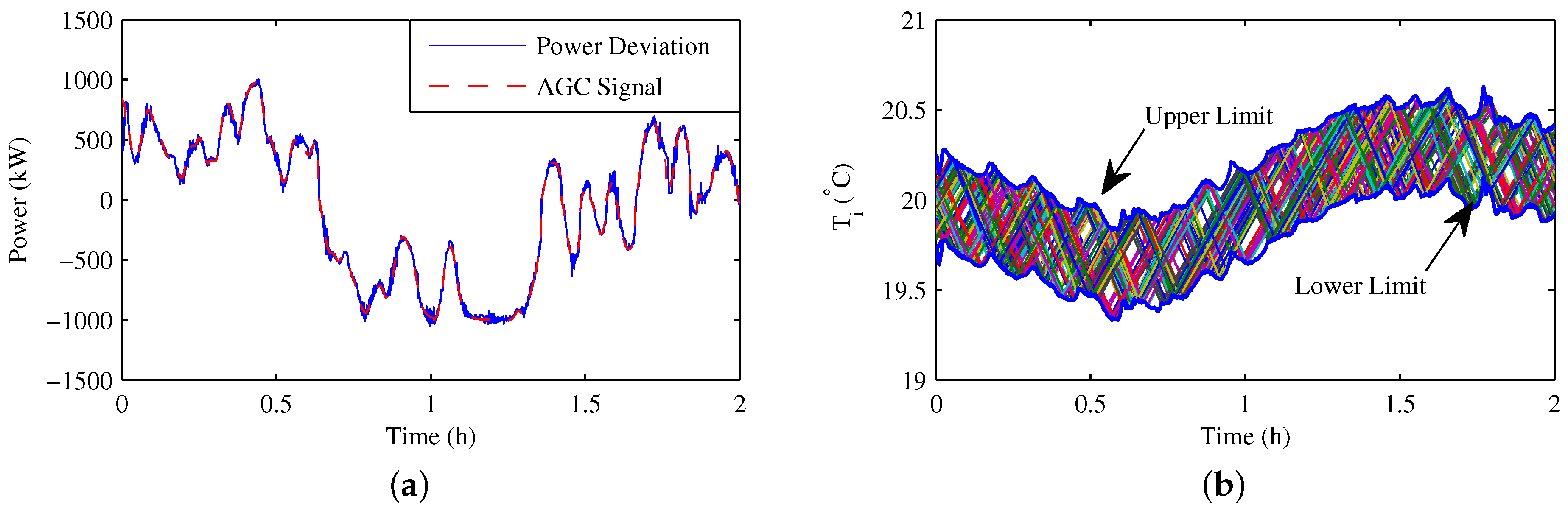
Figure 3.
Diagram of the switched control model.

Figure 4.
The relationship between the RMSE and .

Figure 5.
Diagram of the Fibonacci optimization algorithm.

Figure 6.
Two-stage regulation in a time step [].
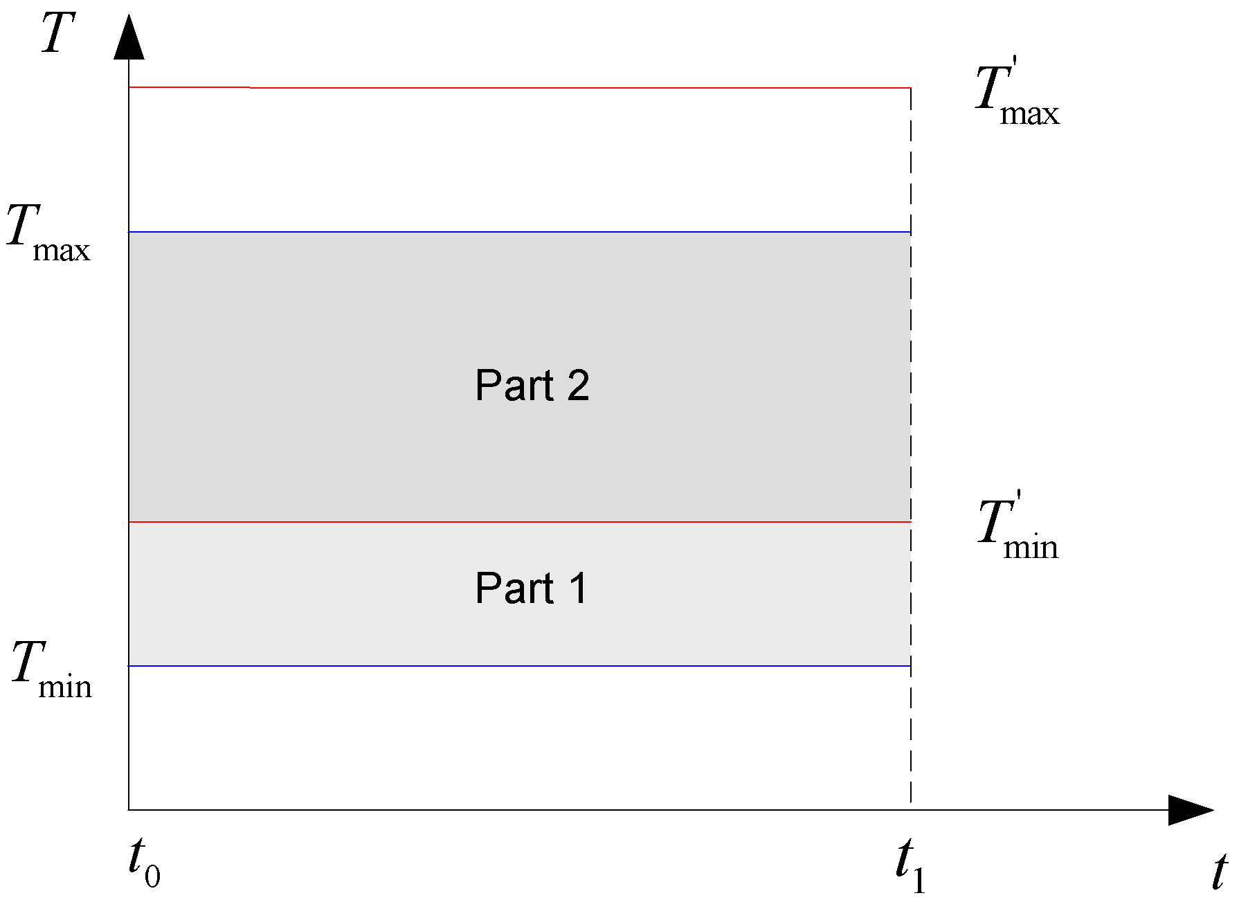
Figure 7.
Flow chart of the switched control strategies.
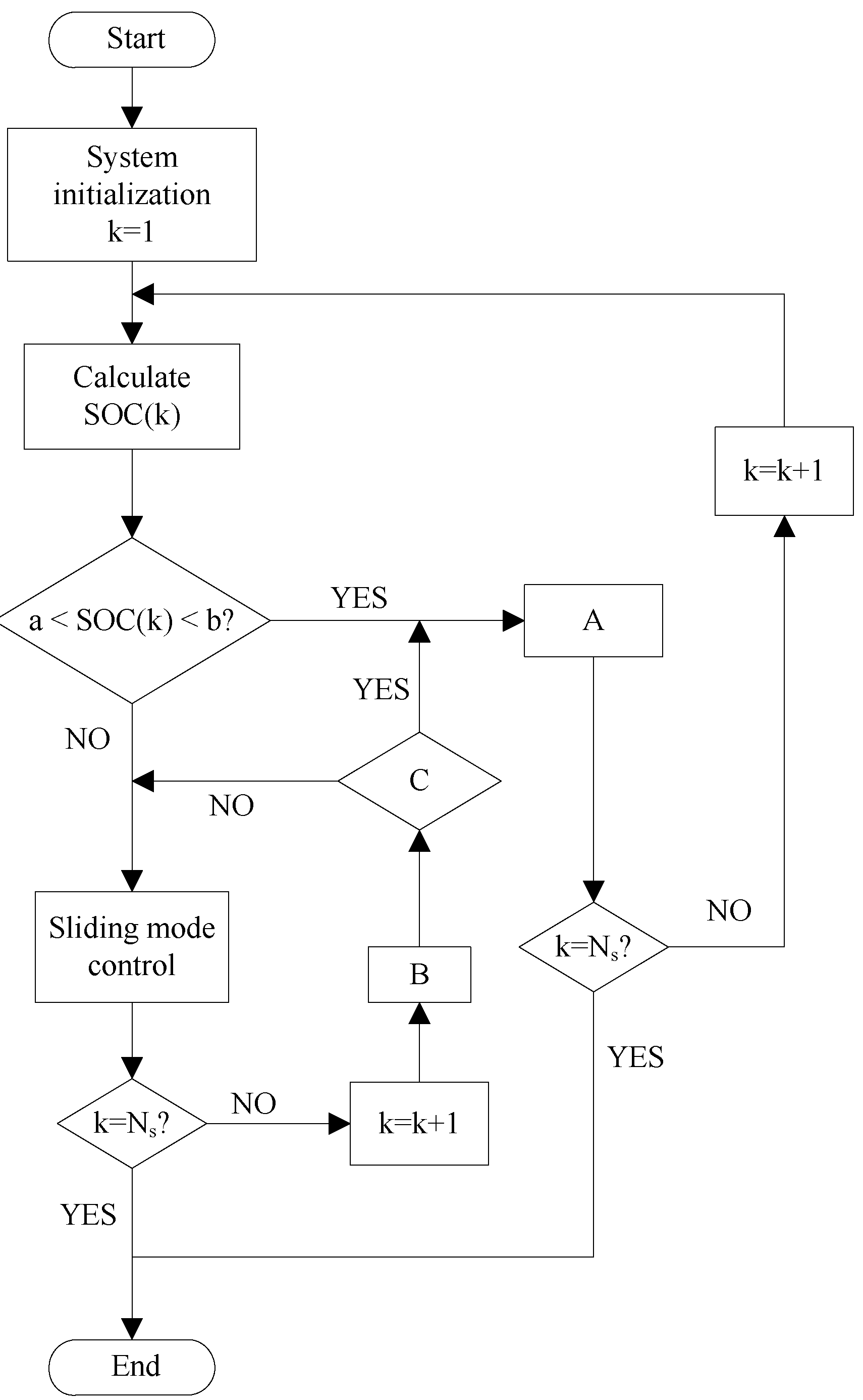
Figure 8.
(a) AGC signal tracking; (b) temperature setpoint trajectory; (c) SOC of Switched Control I.
Figure 8.
(a) AGC signal tracking; (b) temperature setpoint trajectory; (c) SOC of Switched Control I.
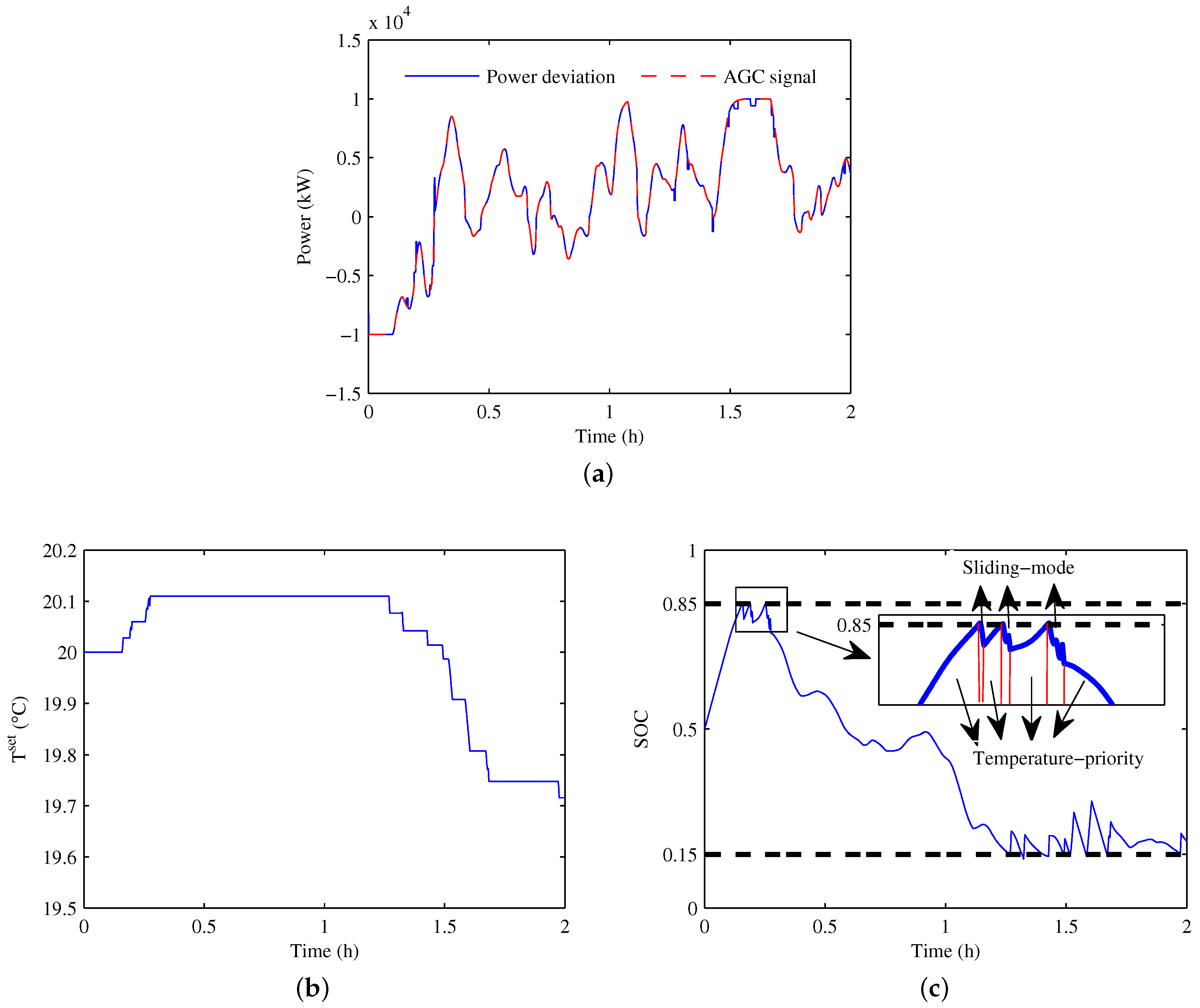
Figure 9.
(a) AGC signal tracking; (b) temperature setpoint trajectory; (c) SOC of Switched Control II.
Figure 9.
(a) AGC signal tracking; (b) temperature setpoint trajectory; (c) SOC of Switched Control II.
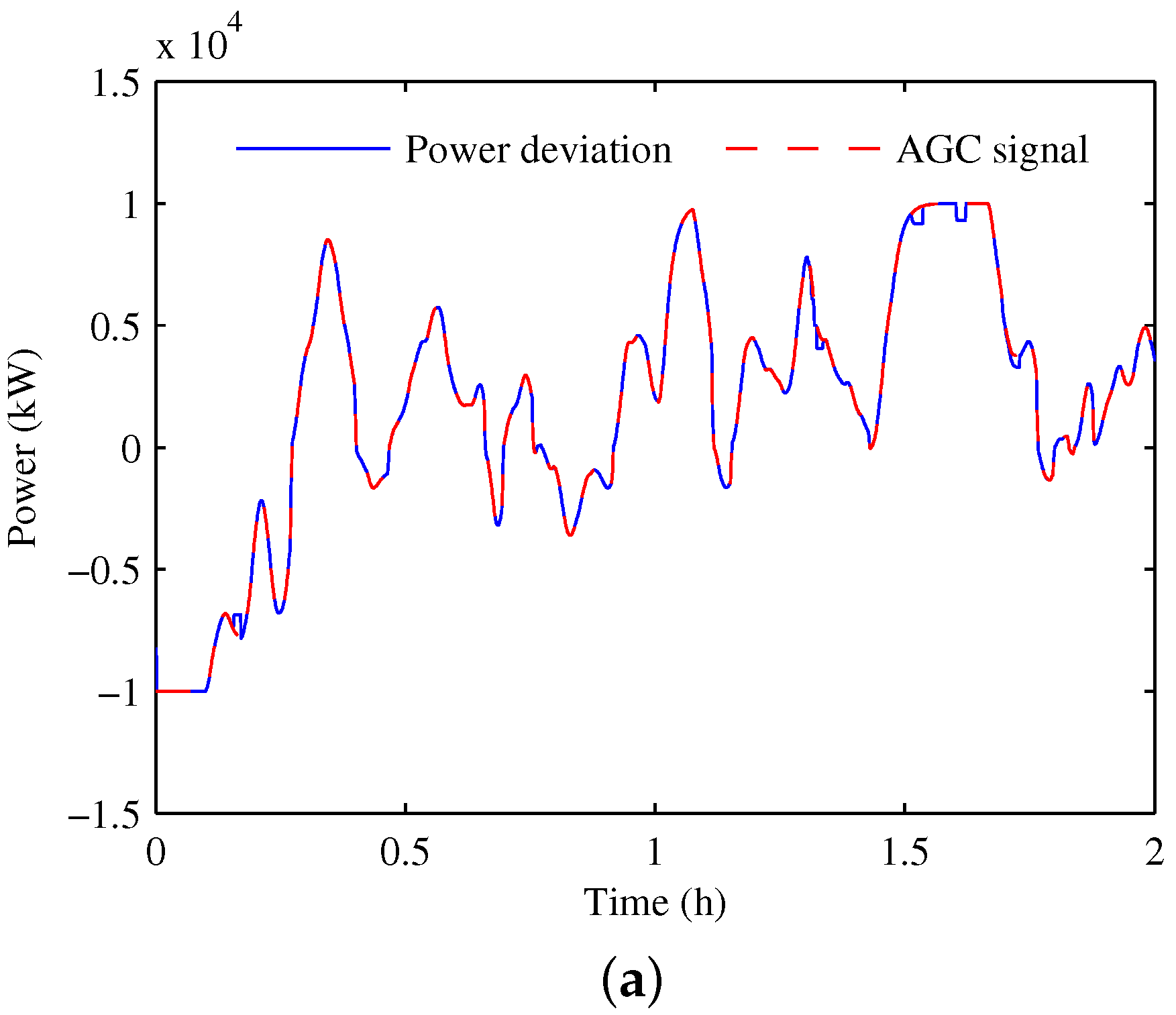
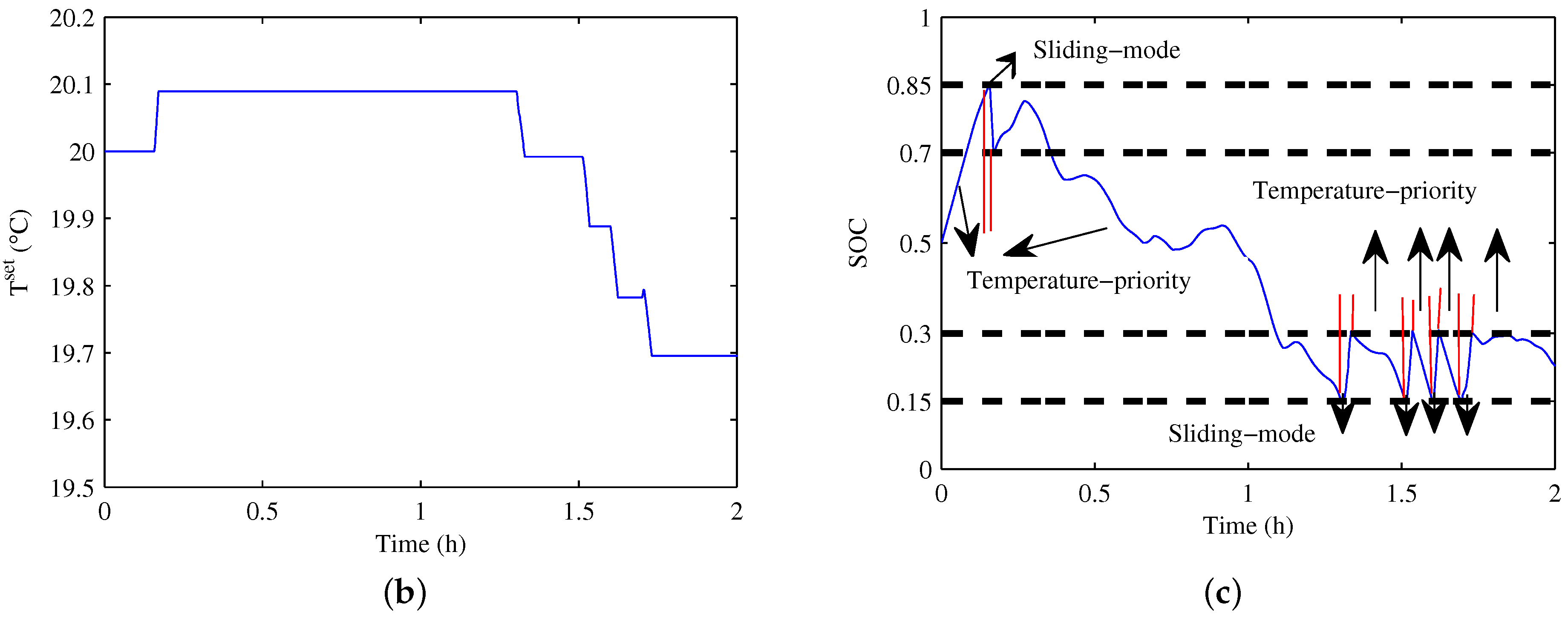
Figure 10.
(a) AGC signal tracking; (b) temperature setpoint trajectory; (c) SOC of Switched Control III.
Figure 10.
(a) AGC signal tracking; (b) temperature setpoint trajectory; (c) SOC of Switched Control III.

Table 1.
Parameter settings.
| Parameters | Meanings | Values |
|---|---|---|
| R | Average thermal resistance | 2 C/kW |
| C | Average thermal capacitance | 2 kWh/C |
| P | Average energy transfer rate | 14 kW |
| efficiency coefficient | 2.5 | |
| Initial temperature setpoint | 20 C | |
| Ambient temperature | 32 C | |
| Thermostat deadband | 0.5 C | |
| Control gain | 8.6 C/h | |
| Boundary layer | 200 kW | |
| h | Time step | 4 s |
Table 2.
The optimal controller gains in different days.
| Day | 1 | 2 | 3 | 4 | 5 | 6 | 7 | 8 | 9 | 10 |
|---|---|---|---|---|---|---|---|---|---|---|
| (C/h) | 8.95 | 8.39 | 9.43 | 8.39 | 8.60 | 8.08 | 8.39 | 8.94 | 8.60 | 8.39 |
Table 3.
Flow chart description.
| Control Strategies | Block A | Block B | Block C |
|---|---|---|---|
| Switched Control Strategy I | Temperature-priority control | Calculate in (14) | ? |
| Switched Control Strategy II | Temperature-priority control | Calculate SOC(k) | c < SOC(k) < d? |
| Switched Control Strategy III | Two-stage regulation | Calculate SOC(k) | c < SOC(k) < d? |
Table 4.
Comparisons with the related works.
| Control Strategies | RMSE | Setpoint Range (C) | The Number of on/off Operations | ||
|---|---|---|---|---|---|
| Average | Maximum | Minimum | |||
| Temperature priority control [23] | 19.15% | 20 | 6710 | 7804 | 5623 |
| Sliding mode control [33] | 2.78% | 19.42∼22.33 | 159 | 211 | 123 |
| Sliding mode control () | 2.51% | 19.41∼22.32 | 159 | 209 | 123 |
| Switched Control Strategy I | 1.59% | 19.64∼22.17 | 299 | 417 | 223 |
| Switched Control Strategy II | 1.15% | 19.61∼22.19 | 307 | 441 | 230 |
| Switched Control Strategy III | 0.94% | 19.66∼22.16 | 363 | 495 | 279 |
© 2017 by the authors. Licensee MDPI, Basel, Switzerland. This article is an open access article distributed under the terms and conditions of the Creative Commons Attribution (CC BY) license (http://creativecommons.org/licenses/by/4.0/).
Share and Cite
MDPI and ACS Style
Ma, K.; Yuan, C.; Yang, J.; Liu, Z.; Guan, X. Switched Control Strategies of Aggregated Commercial HVAC Systems for Demand Response in Smart Grids. Energies 2017, 10, 953. https://doi.org/10.3390/en10070953
AMA Style
Ma K, Yuan C, Yang J, Liu Z, Guan X. Switched Control Strategies of Aggregated Commercial HVAC Systems for Demand Response in Smart Grids. Energies. 2017; 10(7):953. https://doi.org/10.3390/en10070953
Chicago/Turabian StyleMa, Kai, Chenliang Yuan, Jie Yang, Zhixin Liu, and Xinping Guan. 2017. "Switched Control Strategies of Aggregated Commercial HVAC Systems for Demand Response in Smart Grids" Energies 10, no. 7: 953. https://doi.org/10.3390/en10070953
Note that from the first issue of 2016, this journal uses article numbers instead of page numbers. See further details here.