
Analysis of On-Board Photovoltaics for a Battery Electric Bus and Their Impact on Battery Lifespan †

Department of Mechanical and Aerospace Engineering, University of California, Davis, CA 95616, USA
*
Author to whom correspondence should be addressed.
†
This paper is an extended version of our paper published in SAE 2016 World Congress and Exposition
Energies 2017, 10(7), 943; https://doi.org/10.3390/en10070943
Submission received: 17 April 2017
/
Revised: 8 June 2017
/
Accepted: 3 July 2017
/
Published: 7 July 2017
(This article belongs to the Collection Electric and Hybrid Vehicles Collection)
Abstract
:Heavy-duty electric powertrains provide a potential solution to the high emissions and low fuel economy of trucks, buses, and other heavy-duty vehicles. However, the cost, weight, and lifespan of electric vehicle batteries limit the implementation of such vehicles. This paper proposes supplementing the battery with on-board photovoltaic modules. In this paper, a bus model is created to analyze the impact of on-board photovoltaics on electric bus range and battery lifespan. Photovoltaic systems that cover the bus roof and bus sides are considered. The bus model is simulated on a suburban bus drive cycle on a bus route in Davis, CA, USA for a representative sample of yearly weather conditions. Roof-mounted panels increased vehicle driving range by 4.7% on average annually, while roof and side modules together increased driving range by 8.9%. However, variations in weather conditions meant that this additional range was not reliably available. For constant vehicle range, rooftop photovoltaic modules extended battery cycle life by up to 10% while modules on both the roof and sides extended battery cycle life by up to 19%. Although side-mounted photovoltaics increased cycle life and range, they were less weight- and cost-effective compared to the roof-mounted panels.
1. Introduction
The internal combustion engine is a major contributor to greenhouse gas emissions and hydrocarbon pollution across the globe. Motor vehicles account for a major portion of pollutants such as carbon monoxide, nitrogen oxide, and volatile organic compounds [1]. Furthermore, heavy-duty motor vehicles such as trucks and buses are responsible for 30% of all U.S. transportation-related emissions and 60% of particulate matter emissions [2]. Electric and hybrid-electric powertrains are potential technological solutions to reduce vehicle emissions and improve vehicle fuel efficiency. However, heavy-duty electric powertrains require large amounts of stored energy, which can be cost and weight prohibitive [3].
A possible method to reduce battery cost is to supplement the energy storage system with photovoltaic (PV) modules, so that additional power can be generated while the vehicle is on the road. Flexible PV panels allow for vehicle integration without aerodynamic losses or major infrastructural costs [4]. Interest in solar-powered vehicles has been long standing: The first solar-powered “car” dates back to 1955 when General Motors (Detroit, MI, USA) introduced the Sunmobile, a 15-inch long solar-powered vehicle. Various solar-powered or PV-augmented vehicle prototypes were introduced in the following decades [5]. Contemporary research for on-board PV (OBPV) can generally be broken into two groups: integrated PV for consumer vehicles and integrated PV for commercial vehicles.
As consumer vehicles are often parked throughout the day, much of the literature regarding consumer vehicles focuses on analyzing and maximizing collected solar energy for parked vehicles. References [6,7], for instance, analyzed the day-to-day energy collected from parked vehicles to determine the driving distances for PV-augmented hybrid vehicles that minimize both fuel consumption and wasted solar energy. In [8], the relationship between vehicle usage and the impact of OBPV was considered with regards to well-to-wheel vehicle efficiencies and the life-cycle cost of PV cells. Other literature more generally considers the impact of OBPV on fuel consumption and vehicle emissions in an attempt to determine when PV modules will be efficient and inexpensive enough for widespread on-board use [9,10].
In contrast, commercial vehicles are generally operated constantly throughout the day so analysis of OBPV on commerical vehicles tends to focus on powering vehicle components and on the long-term benefits of OBPV. For instance, PV modules have been integrated into health emergency vehicles in order to power medical equipment while the engine is not running and to help guarantee a charge when the vehicle must be started [11]. In another application, OBPV were shown to provide enough energy to power the refrigeration unit on a delivery vehicle [12]. Meanwhile, reference [4] examined the energy collected from roof-mounted PV modules on a diesel-powered bus operating in Poland, noting that such a system “does not require extensive modification to the vehicle electrical system”. Experimental results indicated that the free solar energy, used to power auxiliary electrical loads, would quickly provide a positive return on investment. Reference [13] evaluated the economic feasibility and environmental impact of OBPV for diesel-powered trucks an buses, showing that OBPV could substantially reduce the carbon footprint of heavy-duty vehicles with a payback time of only two to four years.
Still, the majority of the literature for OBPV with commercial vehicles does not consider all-electric powertrains. A small amount of literature exists for light- and medium-duty commercial electric vehicles: for instance, References [14,15] each investigated OBPV for agricultural electric vehicles. The authors have also previously considered OBPV for an electric bus in [16], showing that OBPV could potentially extend battery life or allow for battery size reduction, based on simulation results on a single clear day—this paper represents an expanded version of that analysis. However, the authors are unaware of any other studies directly pertaining to on-board collection of solar energy for heavy-duty electric vehicles.
Given this lack of research, this paper chooses to investigate PV modules integrated on an electric bus for two reasons: one, the large, flat roof and sides of a bus provide ample space on which to attach PV modules and collect solar energy; two, the low speeds and frequent idle time of the bus allow the PV modules to provide a larger share of the traction load compared to, for instance, a truck operating on the highway. This solar energy could be used to extend vehicle driving range. Alternatively, the energy collected from OBPV could be stored instead because buses operate on fixed routes and may not need range extension. The stored solar energy will reduce the depth of discharge of the battery, potentially increasing the battery cycle life and reducing the lifetime cost of the vehicle.
In this paper, both the range-extension and battery cycle life effects of OBPV on electric buses are investigated through a numerical experiment. In Section 2, the models of the various components of the electric bus powertrain and PV system are introduced. In Section 3, a case study of electric buses with and without OBPV is presented. In Section 4, the results from the case study are discussed. Section 5 offers conclusions on this research.
2. Model Formulation
This paper is interested in how PV mounted on-board an electric bus affect that bus’s stored energy consumption and the vehicle battery’s lifespan. Because of the cost to implement and test the proposed system and the time needed to run the battery to the end of its life, simulation is used to assess the performance of OBPV on an electric bus. In this section, the modeling methods and assumptions are described for the vehicle model, motor and power electronics model, battery model, and solar radiation and photovoltaics model.
2.1. Vehicle Model
The goal of the vehicle model is to capture the primary forces on the vehicle while maintaining model simplicity. To that end, a backwards-facing quasi-static vehicle model is used to simulate the vehicle dynamics [17]. It is assumed that the driver accurately follows the reference velocity of the drive cycle. This assumption eliminates the need for a driver model and, because the drive cycle is known, allows the time history of electrical load placed on the electric motor to be calculated in advance.
The vehicle model considers inertial forces on the vehicle and losses due to aerodynamic drag, rolling resistance, and gravitational forces. Other sources of power loss, such as gearbox friction, are neglected. A diagram of the vehicle model and the forces it considers are illustrated in Figure 1. The aerodynamic drag is dependent on air density , frontal area , drag coefficient , and vehicle velocity , as described in Equation (1). The rolling resistance is dependent on total mass M, gravitational acceleration g, road incline , and rolling resistance coefficient , as described in Equation (2). The gravitational force also depends of total mass, gravitational acceleration, and road incline, as described in Equation (3):
In a forward-facing dynamic vehicle model, the drag, rolling resistance, gravitational force, and tractive force from the electric motor would be used to find the inertial force on the vehicle, which would be integrated to find the vehicle velocity [17]. This vehicle model is backwards-facing, so the process is reversed: the inertial force on the vehicle, , is determined from the vehicle acceleration and the vehicle mass:
Then, the inertial force as well as the drag, rolling resistance, and gravitational forces are used to obtain the traction force:
The transmission is assumed to have an efficiency , represented as torque losses. Then, the motor operating speed and the motor torque output are related to the vehicle velocity and traction force by , the gearbox ratio , final drive ratio , and wheel radius :
Then, the power needed to drive the vehicle can be expressed in terms of the motor torque and angular velocity:
indicates mechanical load placed on the electric machine. Positive indicates power consumption during acceleration, while negative indicates power generation during regenerative braking.
This paper considers various battery and PV module configurations, each with different masses. The total mass of the vehicle M is set by a base electric bus mass , constant throughout the experiment, and the battery mass and PV module mass , which are allowed to vary with the size of the battery and size of the OBPV modules. Additionally, the rotational inertia of the bus wheels is accounted for by treating them as equivalent masses [18]:
2.2. Motor and Power Electronics Model
The electrical power consumption or generation of the electric machine, denoted , is calculated from an efficiency parameter and the mechanical load placed on the electric machine. is always less than 1, so the electrical load is found by dividing the mechanical load by the efficiency when motoring and multiplying by the efficiency when generating, as indicated in Equation (10):
Therefore, power is always lost through the motor. The motor efficiency is a function of the motor torque and speed, as described in Equations (6) and (7), and is determined from a static efficiency map:
The efficiency map is obtained from [23], and scaled to the appropriate size using the scaling method in [18]. The modeled vehicle utilizes a 240 kW alternating current (AC) induction motor. The power supplied to the electric machine is provided by the power from the PV panels, , and the battery pack, . In the case of regeneration, power from the electric machine and the PV modules charges to the battery pack. Additionally, there is an auxiliary load which includes loads such as the power for the bus’s heating and air conditioning system, assumed to be a constant 3 kW:
Positive motor power indicates an energy expenditure, while negative power indicates regeneration. Similarly, positive battery power indicates discharge while negative battery power indicates recharging. The busbar operates on direct current (DC). There is assumed to be lossless DC–DC conversion of the PV power and AC–DC conversion of the electric machine load to the voltage of the DC bus. This is depicted for a bus with Rooftop PV modules in Figure 2. PV modules attached to the side of the bus each have their own DC–DC converter and are connected to the DC bus in a similar manner to the rooftop modules.
2.3. Battery Model
2.3.1. Battery Circuit Model
An equivalent-circuit battery model is utilized to simulate the battery performance. The Thévenin equivalent circuit [18] shown in Figure 3 models the battery as a voltage source and resistor and uses empirical data for parameter values. This battery model offers a good balance between model complexity and model accuracy [24]. Parameters are obtained for individual battery cells, which are then stacked in series and parallel to obtain the complete battery pack. The cells are assumed to be identical.
In Figure 3, is the open-circuit voltage (OCV) of a single battery cell, while represents the combined effects of ohmic resistances, diffusion resistances, and charge-transfer resistances [18]. Both the OCV and the internal resistance vary with the battery’s state of charge (SOC), temperature, and current. The relationship between OCV, SOC, and current are obtained from manufacturer datasheets for a lithium-iron-phosphate battery [25]. Although has current and SOC dependencies, it can be treated as constant and still produce suitably accurate results for vehicle simulations [26,27]. This paper takes the cell equivalent resistance to be a constant value of 6 . The resistance and open-circuit voltage also vary with battery temperature, but battery temperature is not considered in this model. Instead, in order to maintain model simplicity, it is assumed that the battery management system keeps the battery at a constant temperature.
The equivalent resistance of the complete battery pack, , is a function of the single-cell equivalent resistance and the number of cells in series, , and in parallel, :
The open circuit voltage of the vehicle battery pack, , is dependent on the open circuit voltage of a single cell and the number of series connections in the battery pack:
The terminal voltage, , and the battery current from the battery pack, , are determined from the open circuit voltage of the battery pack, equivalent resistance of the battery pack, and the power needed for motoring or gained from regeneration:
The terminal voltage is obtained by substituting Equation (15) into Equation (16) solving with the quadratic equation:
The largest possible battery discharge load is 240 kW, per the rated motor power. The solution to Equation (18) will always be real for loads up to 240 kW and for the OCV and equivalent resistance used in this model. With the terminal voltage known, Equation (15) can then be used to determine the current flow from the battery pack.
The instantaneous stored charge, Q, is obtained using the Coulomb counting method [18], where is the initial battery charge:
The initial maximum battery capacity is determined by the rated capacity per cell, , and number of parallel connections:
However, the maximum capacity degrades over time as the battery is used. The instantaneous maximum capacity is denoted . The modeled relationship between the initial and instantaneous maximum capacities are discussed in Section 2.3.2 Battery Health Model.
The state of charge of the battery is an expression of the instantaneous charge as a percent of the instantaneous maximum capacity:
Similarly, the depth of discharge is an expression of the percentage of total capacity that has been discharged:
The C-rate of a battery is a normalized measure of current, such that the complete discharge of the battery over one hour is considered 1 C, and is found by dividing the current by the battery capacity in ampere-hours:
The amount of stored energy used by the battery is found by integrating the power from the battery and the battery losses through the resistor:
Battery weight is determined from the number of cells and the weight per cell. Weight per cell includes the weight of the battery management system, estimated from [28]:
An electric vehicle should have an open-circuit voltage between 300 V and 400 V [29], which is achieved through series connections. Parallel connections can then be used to reach the desired energy storage. The bus in this paper uses a lithium iron phosphate battery cell with nominal OCV, charge, and energy storage of 3.2 V, 2.5 Ah, and 8 Wh, respectively. Battery cells are combined in series and in parallel to achieve a net 962.5 Ah, 338.8 kWh battery pack with a rated OCV of 352 V. The actual OCV ranges from 220 to 374 V depending on operating conditions. This battery size is chosen so that the bus can complete 200 km of driving on a suburban bus drive cycle even when the capacity of the battery has faded by 20%. The parameters of the vehicle model are provided in Table 2.
2.3.2. Battery Health Model
Modeling battery degradation is needed to forecast the long-term performance of the battery and long-term impact that the OBPV have on battery health. The literature typically considers a battery to have reached the end of its life when its maximum capacity has faded to 80% of its original value [30]. The term “cycle life” refers to the number of discharge-and-charge cycles until the battery reaches the end of its life. In this paper, one cycle consists of one day of driving.
Aging of lithium-ion batteries is thought to be caused by formation of cracks in the electrode materials from repeated stress cycles and from the formation of substrates in the chemical reaction pathways [31]. These aging mechanisms are accelerated by high charge and discharge rates, extreme battery temperatures, and deep depths of discharge [32]. However, models of the cell chemistry that include the thermal and stress/strain relationships used to describe aging are computationally intensive and are ill-suited for the analysis considered in this paper [31,33].
A simple aging model is formed by first eliminating aging factors that are not expected to be significant in the experiment. It is assumed that the battery temperature is well-regulated by a battery management system, so the temperature effects of aging are not included in the aging model. Additionally, it will be shown in Section 4.3 that the average charge and discharge rates on the simulated bus are low, and the charge or discharge rates between bus configurations with and without solar power are mostly the same. The impact of large currents on aging are therefore assumed to be negligible as well. On the other hand, enough solar power is collected over the course a day of operation to impact the depth of discharge, so depth of discharge must be considered. Overall, an aging model that only considers depth of discharge is sufficient for this analysis.
This paper uses the cycle life data [34] for the same battery used in the battery equivalent circuit model. The functional relationship between cycle life (CL) and depth of discharge (DOD) is logarithmic in nature [35] and is found by fitting a curve to the manufacturer data. The curve fit proposed in [35] and given in Equation (26) is found to provide the best fit to available data:
Using a least-squares regression, it is found that , and best fits the provided cycle life data. The curve fit results are shown in Figure 4.
Several studies have shown that the Palmgren–Miner (PM) rule, common in fatigue life analysis of mechanical systems, can effectively approximate the battery health over non-uniform charge and discharge cycles [33,36]. The PM rule is a linear damage accumulation model in which each charge and discharge cycle is considered to damage the battery by an amount related to the cycle life at that cycle’s depth of discharge. That is to say, for a given charge and discharge cycle k, the battery will have been discharged to a depth , measured when the bus has finished driving for the day. If continuously charged and discharged to depth , the battery would be able to support cycles before reaching the end of its life, as indicated in Figure 4. Under the PM rule, the damage of that single cycle is assumed to be:
The cumulative damage is an expression of the fraction of a battery’s lifespan that has been used. That is, cumulative damage equal to zero indicates that the battery is at its original health while cumulative damage of one indicates the battery has reached the end of its life. The cumulative damage is measured by summing the damage of individual cycles from the battery’s first use. Thus, the cumulative damage at the completion of cycle k is given by:
In this paper, it is assumed that the maximum capacity is linearly related to the cumulative damage. Then, the maximum capacity after cycle k is determined from the original maximum capacity and the cumulative damage after cycle k. Given that 20% capacity fade indicates end-of-life:
After each simulation cycle, the maximum capacity is updated. The next cycle then measures its state-of-charge and depth of discharge with regards to the new maximum capacity.
It should be noted that this health model relies on regular charge/discharge cycles. That is, it is assumed that the battery is discharged from its initial charge to final charge, without significant charging in between. Similarly, it is assumed that the battery is charged from its final charge back to the original charge without significant discharging in between. Should the charging or discharging become irregular, such as by partially recharging the battery throughout the day, a more complex model of aging would needed [37].
2.4. Solar Radiation and Photovoltaics Model
Accurate assessment of the impact of OBPV requires simulating a representative sample of the weather patterns that a real bus would experience. Additionally, simulation of side-mounted panels requires accurate modeling of different types of radiation in order to model the energy from a panel on the side of the bus facing away from the sun.
PV modules collect three types of radiation: Direct radiation, diffuse radiation, and reflected radiation. Direct radiation travels in a straight line from the sun to the PV module, while diffuse radiation has been scattered by atmospheric particles and approaches from many different directions. On a clear, sunny day, direct radiation makes up the vast majority of the radiation experienced by a PV panel. On the other hand, on a heavily clouded day, the total radiation experienced by a PV panel is entirely diffuse [38]. Reflected radiation is radiation that strikes the PV module after having been reflected off some other surface, such as an asphalt road. The three types of solar radiation are illustrated in Figure 5. Reflected radiation is not considered in this paper.
Although models exist to obtain an estimate of direct radiation on a clear day based on temporal variables and spatial coordinates [39], these models cannot predict the diffuse radiation, due to its dependency on, and the uncertainty of, local weather conditions. Instead, one can use typical meteorological year (TMY) data collected by the National Renewable Energy Lab (NREL) for locations throughout the United States [40]. As its name suggests, TMY data is made of 365 days of weather data selected to cover a range of typical weather phenomena while still matching a region’s monthly and annual average meteorological data. TMY data sets include measurements of the direct normal irradiance (DNI) and the diffuse horizontal irradiance (DHI). DNI is the radiation experienced by a surface held perpendicular to the incoming radiation, while DHI is the radiation that reaches horizontal surface on an indirect path from the sun. The DNI and DHI time-histories from TMY data are used in the experiment for a PV-augmented bus.
In the following subsections, sizing of the OBPV modules is discussed first, followed by modeling of direct radiation on a moving surface and diffuse radiation on a non-horizontal surface. Finally, the model for conversion of solar power to electrical power is presented.
2.4.1. Module Sizing
Two PV system configurations are considered in this paper: one where modules are mounted only on the roof of the vehicle, and another where modules are mounted on the sides and back of the bus as well. The sizing of the modules on the roof and each of the sides is described below.
The size of the PV modules are estimated from the bus geometry and are used to estimate the rating of the roof and side PV systems [41]. The bus is approximated as a box that is 12.9 m long, 2.6 m wide, and 3.4 m tall, with dimensions estimated from manufacturer specifications for an electric transit bus [22]. In order to maximize the impact of OBPV, all possible surfaces should be exploited. It is estimated that the roof-mounted panels, used by both configurations, can cover 60% of the bus roof area . The right and left side modules each cover the same area of their respective sides, and are estimated to cover 40% of the side area , while 75% of the area of the back of the bus is covered in PV panels. These areas are denoted , , , and , respectively:
Each of these areas is then multiplied by the surface power density, , under standard reporting conditions (SRC), which are an operating temperature of C and radiation of = 1000 W/m [42]. The SRC are the laboratory test conditions under which commercial and research PV modules are rated. This produces the rated power, , of the module under SRC as described in Equation (34). To avoid writing redundant equations, the bus surfaces are indexed by a subscript i, with referring to each surface of the bus. Then:
The surface power density is based on manufacturer data [43] for monocrystalline silicone PV cells, which are chosen for their high performance and low aerodynamic profile [4]. Based on these calculations, a bus roof can fit a PV system rated for 3300 W, the right and left sides can each fit a system rated for 2900 W, and the back a system rated for 1100 W.
Similarly, the mass of each PV module is determined from the module area and the area density of a PV module, again based on manufacturer data [43]:
The PV mass is then used in Equation (9) to determine the total vehicle mass.
The parameters of the PV model are provided in Table 3.
2.4.2. Direct Radiation Model
The direct radiation, sometimes called the beam radiation, represents the radiation that travels on a direct path from the sun to the PV panel. When the direct radiation strikes a PV panel tilted away from the direct radiation’s path, only the component of the direct radiation that is perpendicular to the panel is converted into electrical energy. For direct normal irradiance with magnitude and an angle of incidence , the panel experiences beam radiation according to:
Alternatively, the direct radiation could be defined as a vector pointing towards the PV module in a 3D coordinate system. Then, a unit surface normal vector could be defined for the PV module. This paper uses a convention for the normal vector such that a horizontal panel has a normal vector pointing directly up and a panel that is perpendicular to the direct radiation has a normal vector pointing towards the sun. Then, the incident beam radiation could be obtained by taking the negative dot product of and , with the caveat that if the panel is facing away from the direct radiation, the radiation is zero, rather than negative:
This method is illustrated in Figure 6.
The PV modules under consideration in this paper are pitching and turning as the bus pitches and turns, changing the angle of incidence on each surface of the bus at each time-step. In order to obtain the incident beam radiation on moving surfaces, the following method is proposed: the direct radiation is first placed into a global coordinate system and then transformed into a local coordinate system oriented with the moving bus. Meanwhile, surface normal vectors are defined in the local coordinate system for each PV module on the bus. Then, the incident beam radiation on each surface is obtained using Equation (37). This process allows the incident beam radiation on each surface of the vehicle to be obtained at each time-step of the simulation.
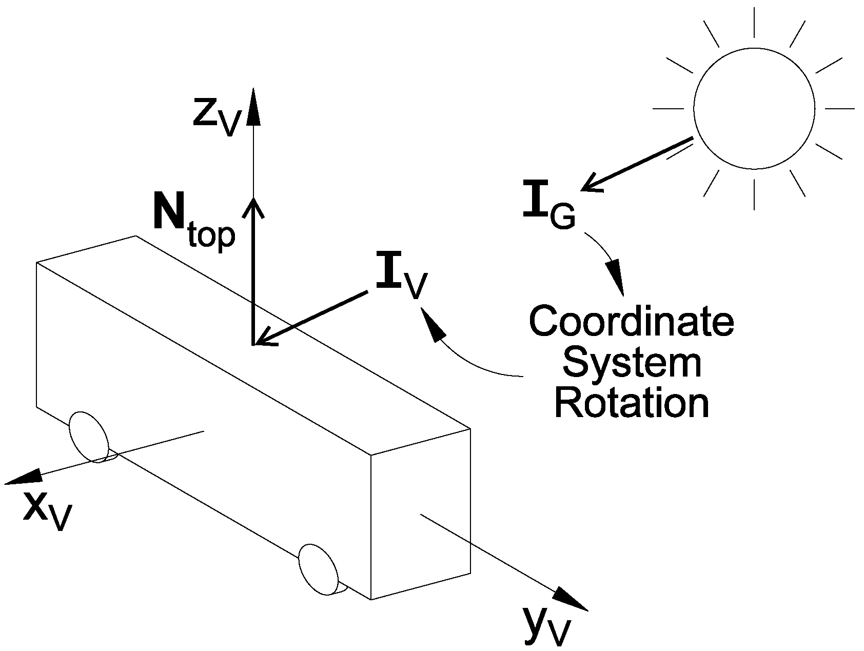
The global coordinate system assigns the east/west direction to the x-axis, the north/south direction to the y-axis, and the vertical direction to the z-axis. The azimuth angle is the angle of the sun along the horizon, where an angle of zero indicates north. The zenith angle is the angle of the sun off of the vertical axis. The direct radiation vector in this coordinate system is , where the subscript G indicates the global frame. The global coordinate system is illustrated in Figure 7.
The azimuth angle and zenith angle are obtained based on the latitude, longitude, time of day, and time of year at each time-step of the simulation. The process for finding the azimuth and zenith angles is given in [44]. For direct normal irradiance with magnitude DNI, obtained from TMY data, and azimuth and zenith angles and , the direct radiation is put into vector form in the global coordinate system such that the direct radiation vector points towards the earth, according to Equation (38):
Here, the variable DNI indicates the magnitude of the direct normal irradiance. The negative signs in Equation (38) result from being defined as traveling from the sun to the bus.
Next, the vehicle coordinate system is defined such that the first coordinate indicates the lateral direction, the second coordinate indicates the longitudinal direction, and the third coordinate indicates the vertical direction. For each axis, the rightward, forward, and upward directions are positive, as shown in Figure 8.
Then, for heading and pitch angle , where indicates north and indicates a horizontal surface, is rotated as shown in Figure 9a,b. These rotations are carried out using the two rotation matrices and , given in Equations (39) and (40), to obtain the direct radiation vector in the vehicle coordinate system, . denotes the direct radiation vector in the intermediate coordinate system between the global and vehicle coordinate systems:
The unit normal vectors for the PV module surfaces are then defined for each surface of the bus. The unit normal vector for the top surface is a unit vector pointing straight up, the unit normal vector for the right-side surface is a unit vector pointing directly to the right, and so on. These unit normal vectors are given by Equations (42)–(45):
Although this model only uses surfaces with normal vectors along the coordinate system axes, this method could be used for surfaces facing any arbitrary direction.
Then, per Equation (37), the incident beam radiation on each surface is given by:
However, some amount of the direct radiation on the vehicle is expected to be blocked by things such as buildings or overhead trees. An additional efficiency factor is introduced to represent losses from shading of the PV modules:
Based on experimental results in [4], it is estimated that . In other words, 25% of all direct radiation is considered lost to shading. Although estimating as constant will reduce the model accuracy on small time scales, it is sufficient for measuring the total radiation over longer time scales, such as an hour or a day.
2.4.3. Diffuse Radiation Model
TMY data provide diffuse radiation as diffuse radiation on a horizontal surface. However, this paper considers PV modules mounted on the sides and back of a bus, which are decidedly not horizontal. Additionally, the pitch motion of the bus is considered, so the roof- and back-mounted PV panels experience further tilt. A way to convert diffuse horizontal radiation into diffuse radiation on a tilted surface is needed.
Reference [45] compared the accuracy of several diffuse radiation models. Among them is the isotropic sky diffuse model, which models diffuse radiation as uniformly distributed across the sky. Under this modeling assumption, the diffuse radiation on a tilted surface is given by:
where DHI denotes the magnitude of the direct horizontal irradiance and denotes the tilt angle. This is the simplest of sky diffuse models and the foundation upon which other models are built. More complex models include effects such as horizon and circumsolar brightening but often use empirical lookup tables that add to the model’s computational load and rely on additional parameters such as the angle of incidence and zenith angle. The simplicity of the isotropic model makes it much more suitable for a vehicle simulation.
This model is applied to each surface. By using the isotropic model, only pitch angle is needed to determine the diffuse radiation on each module. Knowledge of the bus heading or the sun’s position in the sky is not necessary. The top panel is tilted only with respect to the pitch angle. The side panels each remain vertical for the entire experiment, as it is assumed that the roll angle is constant and equal to zero. The back panel is tilted by to start, and is subject to additional tilt based on the pitch angle. This shown in Figure 10 and described in Equations (49)–(52):
2.4.4. Efficiency Modeling
Once the incident beam and diffuse radiations on each surface have been found, the total radiation on each surface is obtained by adding them together:
With the total radiation on each surface known, a model must be formed to relate the solar radiation to the electrical power extracted from each module.
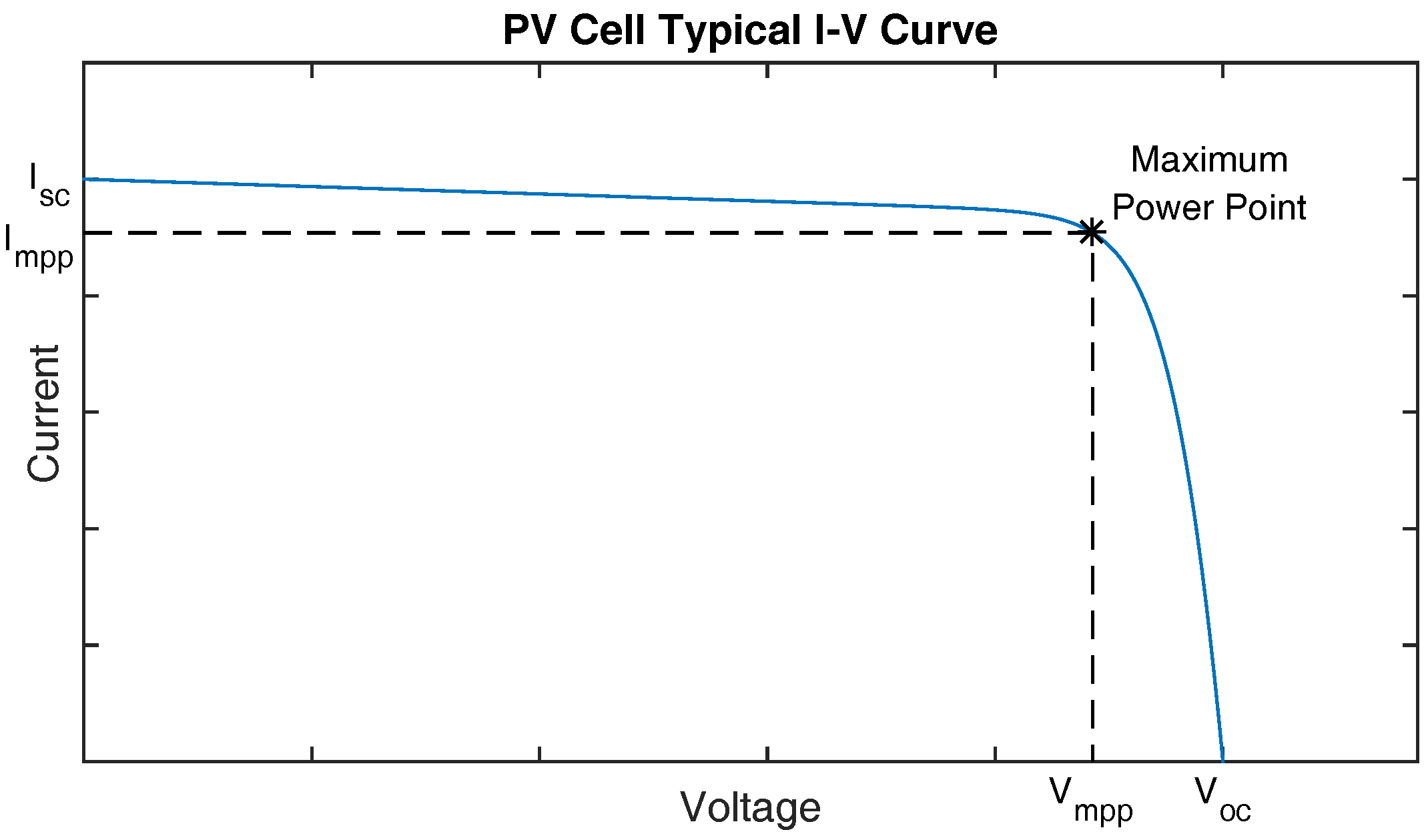
The fundamental behavior of a PV cell can be modeled as a circuit with a current source, an ideal diode, and series and shunt resistances, as shown in Figure 11 [46]. Solving for the terminal voltage and current using the method described in [47] produces an I–V curve with a shape typified by Figure 12. For any given operating condition, PV modules have an ideal operating point, known as the maximum power point (MPP). The power, voltage, and current at the MPP can vary considerably with temperature and radiation. However, extensive literature exists showing how the MPP can be tracked in order to maximize PV performance under variable conditions. Reference [48], for instance, reviewed 19 distinct methods of MPP tracking that have been studied in academic literature.
In order to ensure as much solar energy as possible is utilized, it is assumed that the MPP is tracked on each PV module. Although this is a strong assumption given the difficulties in tracking the MPP for a system that may be partially shaded [49], the shading efficiency in Equation (47) is expected to encompass any losses from failing to track the MPP accurately. The DC–DC converters described in Section 2.2 and shown for the rooftop module in Figure 2 are used to track the MPP of the top and side modules. By assuming the MPP is tracked accurately, it is only necessary to model the behavior of the peak power value rather than the behavior of the PV module as a whole. In this paper, the temperature and radiation dependencies of the maximum power are considered.
It can be assumed that the peak power value varies linearly with temperature according to a peak power temperature coefficient, [42]. represents the fractional change in performance of the module as the actual cell operating temperature T deviates from the SRC temperature. In this paper, cell operating temperature is described by the thermal model presented in [42]. This thermal model estimates the operating temperature T from the current total radiation and air temperature as well as the nominal operating cell temperature (NOCT) under a nominal thermal environment: radiation of 800 W/m and ambient air temperature of 20 C:
It should be noted that while SRC represents standard lab conditions, the nominal thermal environment in [42] represents the conditions that the PV module is typically subjected to once installed outside. The ambient air temperature is acquired from TMY data. is taken to be C and the NOCT is taken to be C, based on literature regarding mono-crystalline silicon PV cells [50,51]. Manufacturer datasheets may provide this information as well.
The peak power value is modeled as varying linearly with radiation exposure. This is a first-order accurate model, per [42], and is seen by the authors as a suitable trade-off between complexity and accuracy. As discussed previously, the PV system is rated at test conditions of W/m. Thus, the electrical power produced at is given by the rated PV power times the ratio of the current total radiation and the SRC radiation.
The temperature effects described previously are then incorporated to form Equation (55), which describes the electrical power produced by a PV system subject to variations in temperature and radiation exposure:
The shading factor in Equation (47) is expected to account for some potential losses like the MPP tracker finding a local (rather than global) optimal operating point. Additional sources of module inefficiency, such as soiling or degradation of the modules, are not considered in this study but will be the subject of future work.
3. Case Study
In this section, a case study is laid out to assess the impact of PV on the electrical energy consumption of the bus and the aging of the bus battery. The following subsections describe the different bus configurations, the simulated geographic location, drive cycle, bus route, and time of operation examined in the case study.
3.1. Bus Configurations
As discussed in the Section 2, two different configurations of OBPV were simulated. One configuration, hereby referred to as the “Rooftop PV” configuration, has PV modules mounted to the roof of the bus only. The other configuration, hereby referred to as the “Full-Body PV” configuration, has PV modules mounted to both the roof, sides, and back of the bus. These configurations are listed in Table 4.
Simulation with these two configurations would reveal how integrated PV power can improve battery life and extend vehicle range. However, it is also true that battery cycle life and vehicle range could be extended by simply using a larger battery. In order to assess how the benefits of integrated PV hold up against the benefits of increased battery capacity, two additional bus configurations are proposed.
The first additional configuration has no PV modules, but the battery pack has been enlarged to have a total energy capacity of 341.9 kWh by adding an additional set of battery cells in series (, ). This corresponds to adding batteries equal in weight to the weight of the Rooftop PV module. This configuration is hereby referred to as the “Equal Weight” configuration.
The second additional configuration has no PV modules, but the battery pack has been enlarged to have a total energy capacity of 356.6 kWh by adding six battery cells to each parallel set and by adding four additional battery sets in series (, ). This corresponds to adding batteries whose cost is approximately equal in to the cost of roof PV module. The cost of lithium-ion batteries and PV modules are estimated from industrial average prices [52,53]. This configuration is hereby referred to as the “Equal Cost” configuration.
Simulation of these additional configurations allow the benefits of PV to be compared fairly to batteries. A nominal bus with no PV and with the original battery pack is simulated as well.
3.2. Simulation Location
The impact of OBPV on an electric bus depends on the local weather conditions and the geographic location of the bus’s route. Clearer locations, locations closer to the equator, and locations with a higher elevation are exposed to more solar radiation, resulting in a greater impact on the vehicle’s energy consumption. Additionally, the performance PV panels mounted on the side or back of the bus depend on the chosen route. For instance, side-mounted panels operating on a bus near the equator will collect more energy if the route is primarily in the north/south direction, perpendicular to the direction of travel of the sun and therefore exposed to more solar radiation.
This paper considers a PV-augmented bus in Davis, CA, USA. Davis experiences hot, clear summers and cool, rainy winters. It is at roughly sea level and, at N W, is slightly south of the average latitude of the contiguous United States. The annual solar insolation on an optimally tilted plane in Davis is approximately 2100 kWh/m [54]. The TMY data for Sacramento International Airport (approximately 18 km away from Davis) is used to estimate a full 365 days of weather [55].
3.3. Drive Cycle
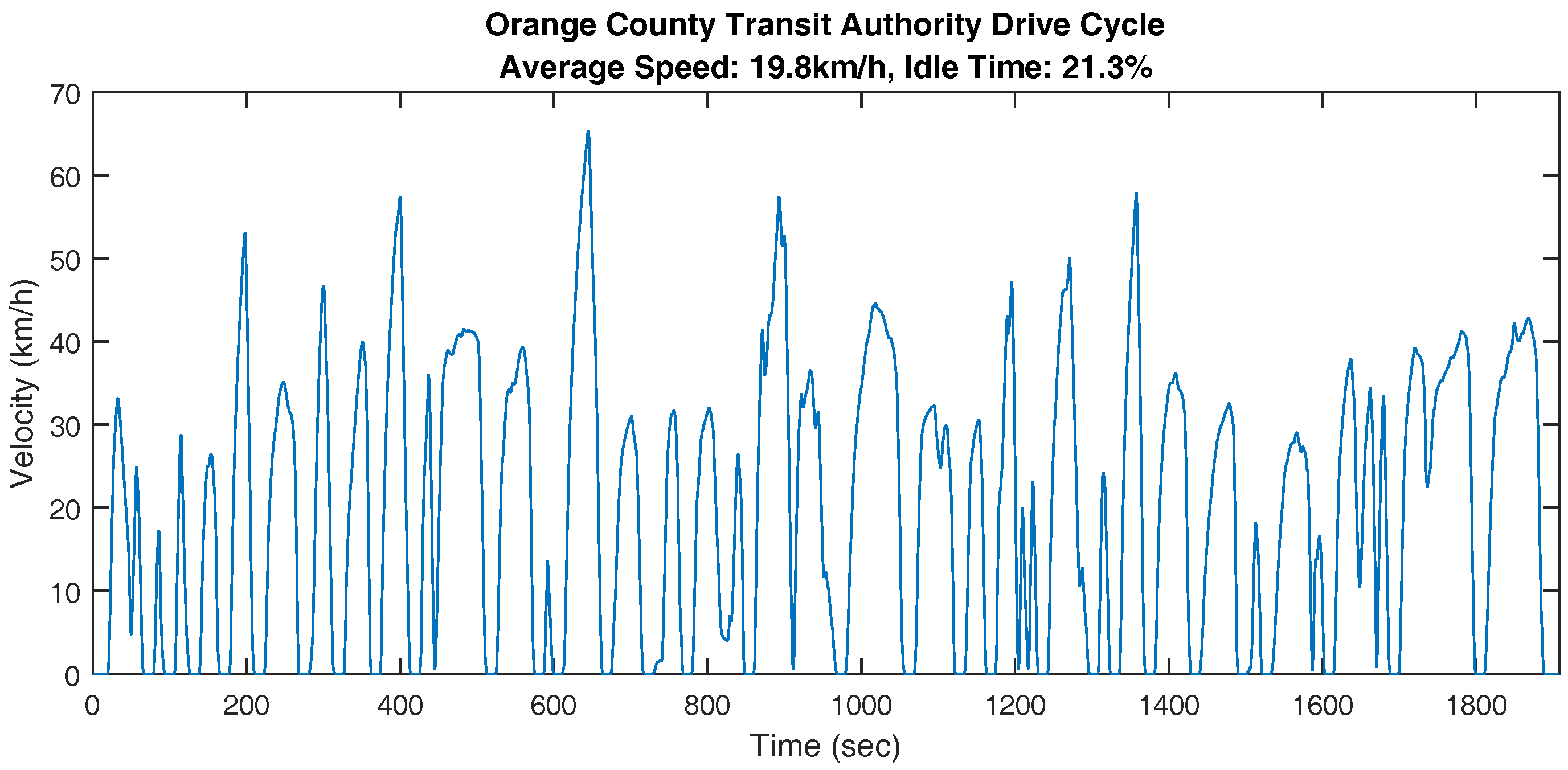
The electric bus was simulated on the orange county transit authority (OCTA) drive cycle [56]. This drive cycle is an experimentally gathered velocity profile for a suburban bus in Orange County, CA, USA. The velocity profile is shown in Figure 13. This cycle was repeated several times until the desired route length was reached.
3.4. Route
The electric bus is set to follow the UC Davis Unitrans O-Route bus route, at a pace set by the OCTA drive cycle. Depicted in Figure 14, the route spends roughly equal time heading north, south, east, and west. The elevation was assumed to be constant. With the assumption of constant elevation (and therefore road grade/pitch angle set to zero for the duration of the experiment), the choice of route does not impact the results for the bus with roof-mounted panels only. However, the route choice still impacts the performance of the side- and back- mounted panels.
The degree of impact of OBPV was expected to vary with the usage patterns of the bus: different daily driving distances have different depths of discharge, resulting in different aging of the battery. In order to fully evaluate the impact of OBPV, each configuration of the bus was simulated for daily driving distances ranging from 120 to 200 km. On the OCTA drive cycle, this corresponds to daily driving durations of 6 to 10 h. The longest daily route length, 200 km, corresponds to the furthest the nominal bus can drive once its battery has reached the end of its life—when its capacity has faded by 20%.
3.5. Simulation Timespan
The simulated bus begins its route each day at 7:00 a.m. Repeated simulations were carried out to find the battery cycle life for each configuration operating and daily driving distance. In the case of the Rooftop PV and Full-Body PV configurations, the daily weather conditions from TMY data was used chronologically. The repeated simulations were also used to measure the electrical energy collected by the PV modules on each day of the typical meteorological year.
4. Results and Analysis
The results of the case study are organized as follows: first, the range extension provided by the electric bus is estimated. Next, the results are used to measure the amount of electrical energy that was collected per year from an OBPV system, compared to the annual consumption of electric energy by the bus. Third, the results are used to determine the impact of OBPV on battery aging, as compared to other methods of increasing battery life.
4.1. Range Extension
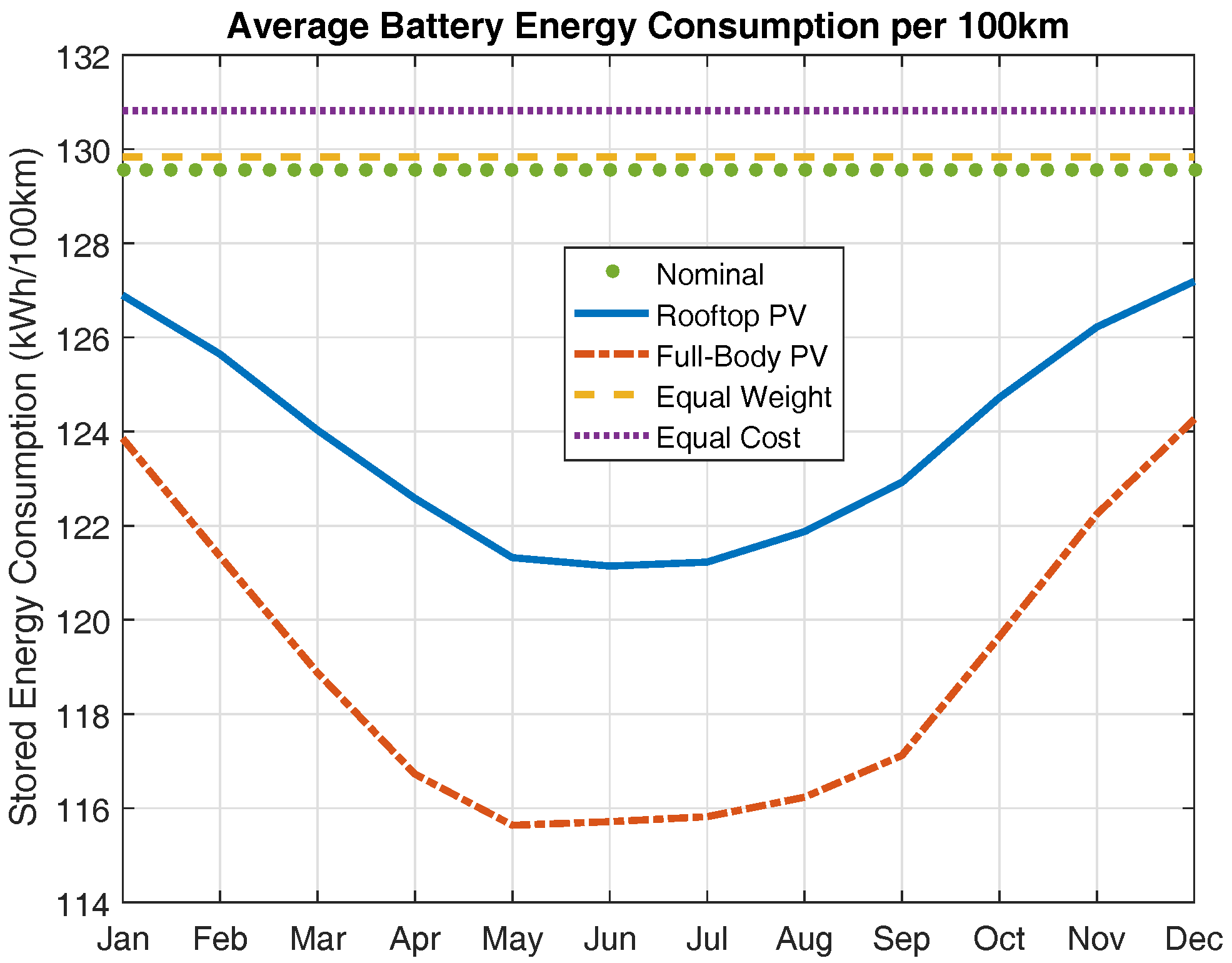
During the experiment, the nominal bus configuration used 129.6 kWh/100 km on average. The Rooftop PV configuration also used 129.8 kWh/100 km while the Full-Body PV configuration used 130.2 kWh/100 km, the Equal Weight configuration used 129.8 kWh/100 km, and the Equal Cost configuration used 130.8 kWh/100 km. However, the Rooftop PV and Full-Body PV configurations met the bus power request using both battery stored energy and power from the PV modules. The battery stored energy consumed per 100 km was 123.8 kWh/100 km on average for the Rooftop PV configuration and 118.9 kWh/100 km on average for the Full-Body PV configuration, although these values varied with the amount of usable sunlight. Figure 15 shows the consumption of battery stored energy per 100 km for each configuration as it varied by month.
Using these data, the range extension provided by either PV configuration compared to the nominal bus was estimated. Results are presented as additional range per 100 km driven by the nominal bus. On an average day, Rooftop PV could extend driving range on by 4.7 km per 100 km driven, while PV modules on the roof and sides could extend driving range by 8.9 km per 100 km driven. However, the amount of solar energy collected daily varied considerably with time of year and weather conditions—the Rooftop PV could provide as little as 1.5 kWh or as much as 19.2 kWh of electrical energy, while a bus with both roof and side modules could get as little as 3.0 kWh or as much as 33.4 kWh. In the worst case (an overcast winter day), Rooftop PV could extend the range by only 0.3 km per 100 km driven, while PV modules on the roof and sides could extend range by 0.6 km per 100 km driven. On the other hand, in best-case conditions (a clear summer day), range could be extended by 7.6 km per 100 km driven for Rooftop PV and by 13.4 km per 100 km driven for roof and side PV. A histogram of the range extension provided by OBPV is shown in Figure 16. The implementation of OBPV had the clear potential to extend vehicle driving range, as on the majority of days the bus range can be extended by several kilometers. However, the minimal energy collected in the worst-case weather conditions, and the number of days that OBPV provides only a negligible increase in range, indicate that OBPV was not a robust means to extend range every day of the year. The inclusion of side-mounted PV panels helps mitigate this somewhat, but still has some days with negligible range extension.
4.2. Photovoltaic Energy
The intensities of solar radiation reaching the bus roof and bus sides were compared in terms of daily irradiance and monthly insolation. Figure 17a shows the simulated radiation that reaches the bus on a fairly typical day. The side PV modules experienced more variation than the roof PV modules due to the changing bus orientation and also experienced a decrease in radiation during midday, when the sun was close to directly overhead. The side modules experienced less radiation in general because they could not always be exposed to direct radiation. However, near sunrise and sunset when the sun was low in the sky, sunlight reached the side modules at a more direct angle, such that the side modules experienced more radiation than the roof module. Figure 17b shows the total solar insolation that reached the panels each month. In Figure 17b, the total radiation on the side modules is found by taking a weighted average of the total radiation on the right, left, and back modules:
The insolation is found by integrating the radiation with respect to time. Because the bus traveled north, south, east, and west roughly equally, the insolations on the right, left, and back PV modules were approximately equal to each other regardless of time of year.
The sun is lower in the sky in winter months compared to summer months, so solar radiation approached the side modules at a more direct angle. In addition, greater cloud cover in the winter months meant that the diffuse radiation made up a larger portion of the total radiation. This resulted in less discrepancy between the Rooftop PV modules and side PV modules during winter months compared to summer months. The total yearly solar insolation was 1480 kWh/m on the roof module and 640 kWh/m on the side modules.
Assuming the PV modules could continue to collect energy and charge the battery while the bus was not in operation, the roof-mounted panels collected a total of 4560 kWh of electrical energy over one year, while the side-mounted panels collected a total of 4321 kWh of energy. Figure 18 shows the electrical energy from PV modules by month. The electrical energy is found by integrating Equation (55), where the solar radiation and ambient temperature for each day of the year are obtained from the NREL’s TMY data [55]. Because the side modules covered a larger area than the rooftop modules, they produced a comparable amount of electrical energy to the rooftop modules despite their lower annual insolation.
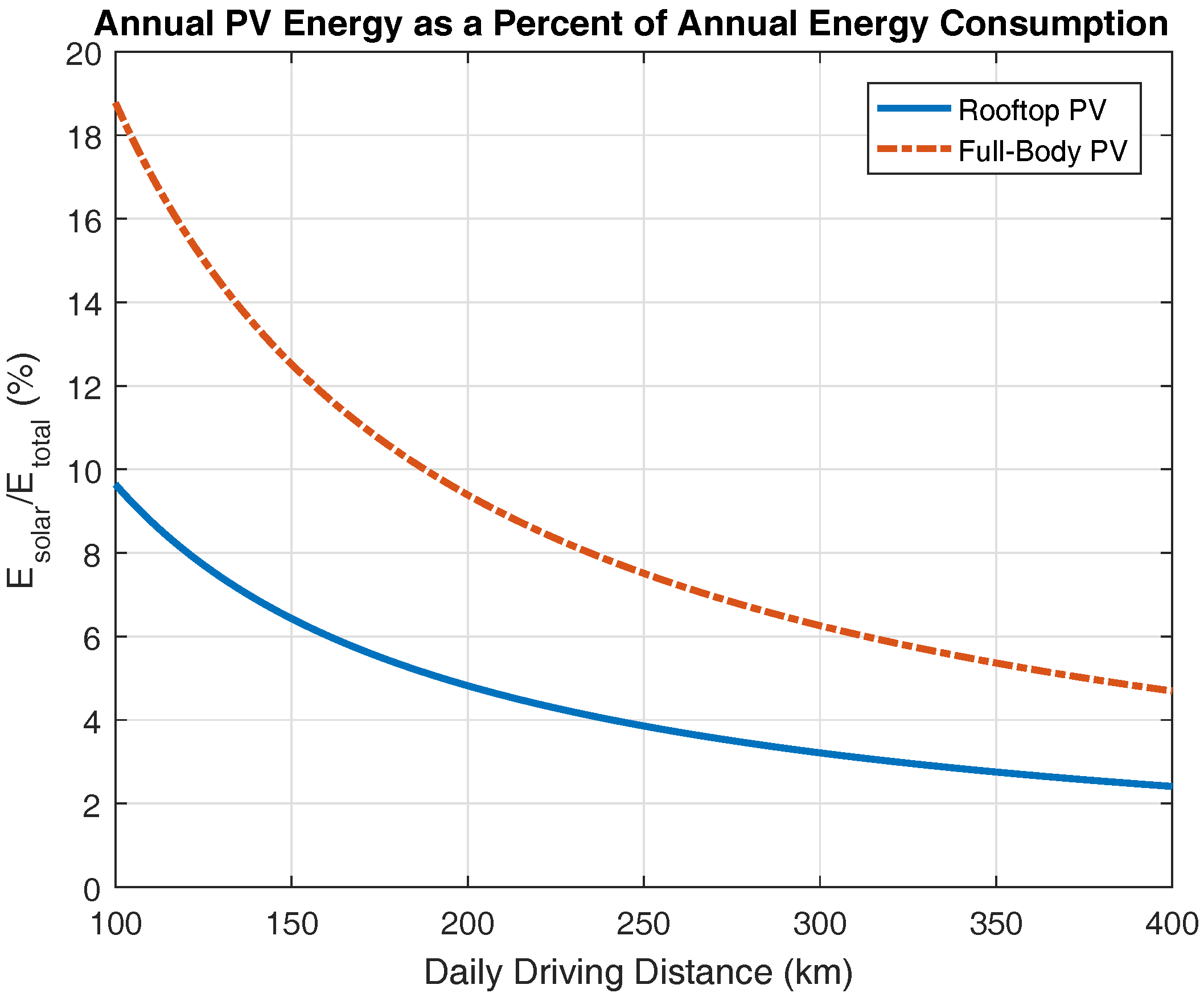
Using the fuel economy results presented earlier, one can estimate the portion of the annual electrical energy consumption of the bus that the PV modules can provide for various daily route lengths. For instance, if a bus is driven 150 km each day, Rooftop PV modules could provide up to 6.4% of the electrical energy, while modules on the roof and sides could together provide up to 12.5%. The relation between this percentage and the average daily driving distance is illustrated in Figure 19.
An interesting finding was that although the side-mounted PV panels provided less power in summer months, they provided as much or more power than the Rooftop PV modules during the winter months. This was because, in winter months, the earth is tilted away from the sun, resulting in the radiation having a more direct path to the side modules than in summer months. Although the side PV modules were less efficient on a per-area basis, they reduced the variability in daily energy collected between summer and winter months.
The payback time can be computed for the top and side PV modules using the commercial off-peak cost of energy in Davis, $0.23 per kWh [57]. Using the industrial average price per watt of solar panels, it is estimated that the rooftop module would cost $6247, while the side modules would cost $13,139 [53]. Then, the rooftop panels are expected have a payback time of six years, while the side panels are expected to have a payback time of 13 years and three months. These payback times are longer than the amount estimated in [4,13] due to the lower price of electric energy compared to diesel fuel. For payback times of this length, it is questionable whether a manufacturer would want to go ahead with PV integration. However, these payback times do not account for any incentives that local government might offer for solar installation, nor do they account for the value added from extending the battery cycle life, which will be discussed in Section 4.3.
4.3. Battery Aging
Repeated simulations were carried out for each configuration to find the battery cycle life associated with each configuration and route duration. In this section, one “cycle” refers to one day of driving. The nominal, equal weight, and equal cost configurations did not have any weather-dependent parameters, so the only variation from one simulation to the next was the maximum battery capacity. On the other hand, the Rooftop PV and Full-Body PV configurations had weather conditions that changed daily in addition to the changing maximum battery capacity. These experiments were carried out using chronological TMY data.
Before proceeding to the battery aging results, some of the aging modeling assumptions are verified. The battery aging model assumed that the charge and discharge rates, as well as the difference in charge and discharge rates between configurations, would be small enough that the aging model would only need to consider the depth-of-discharge per cycle. It was observed from the results that the average absolute C-rate for the nominal bus was 0.169 C, while it was 0.166 C for the Rooftop PV configuration and 0.165 C for the Full-Body configuration. These rates are low and near 0.5 C, the C-rate of the test data in [34]. Additionally, the maximum discharging C-rates were 0.777 C, 0.768 C, and 0.764 C, respectively, while the maximum charging C-rates were 0.968 C, 0.977 C, and 0.992 C. Because the C-rates were low and near the C-rate of the empirical cycle life data, and because the differences in C-rate between the configurations were minimal, the assumption that charge and discharge rates could be neglected from the aging model was considered valid.
Figure 20 shows the aging of the five different configurations for a 160 km daily bus route. The battery for the nominal configuration aged the fastest, reaching its end-of-life after approximately 6000 charge-and-discharge cycles—or rather, approximately 6000 days of driving. The Full-Body PV configuration aged the slowest, followed by Rooftop PV and then the two extra-battery configuration. For each configuration, as the maximum storage capacity of the battery decreased with each day of driving, it was discharged to greater depths, which, in turn, caused each cycle to do more damage.
Figure 21a shows the cycle life for each configuration as it varies with route length, while Figure 21b shows the increase in cycle life of each configuration over the nominal configuration at each route length. Although the marginal cycle life for each configuration increased with decreasing route length, the percentage increase in cycle life was greater for longer routes. The Full-Body PV configuration increased the battery cycle life the most, followed by the Rooftop PV, then the Equal Cost, and finally the Equal Weight configuration.
Increased cycle life on its own is not necessarily a good metric for each configuration’s performance. Each configuration would have different drawbacks, such as added mass, size, or installation cost. The additional benefits of each configuration should therefore be compared to the additional penalty incurred by implementing that configuration.
This paper first considers the marginal mass of each configuration. If the added PV modules or battery cells add too much weight, it might require the manufacturer to redesign other components of the bus or reduce the allowable number of passengers. The marginal mass of each configuration is summarized in Table 5.
Additionally, each configuration was looked at in terms of the effort required to implement that configuration. “Effort to implement” might include cost to install each configuration, ongoing maintenance costs, or additional hardware, such as a larger battery management system. This paper considers the estimated marginal cost of the configuration, in terms of the industrial average price per watt of PV panels and price per kilowatt-hour of lithium-ion batteries, to be a reasonable proxy variable for “effort to implement”. The price per kilowatt-hour for lithium-ion batteries is provided by [52], while the price per watt of PV systems is from [53]. The marginal cost of each configuration is summarized in Table 5.
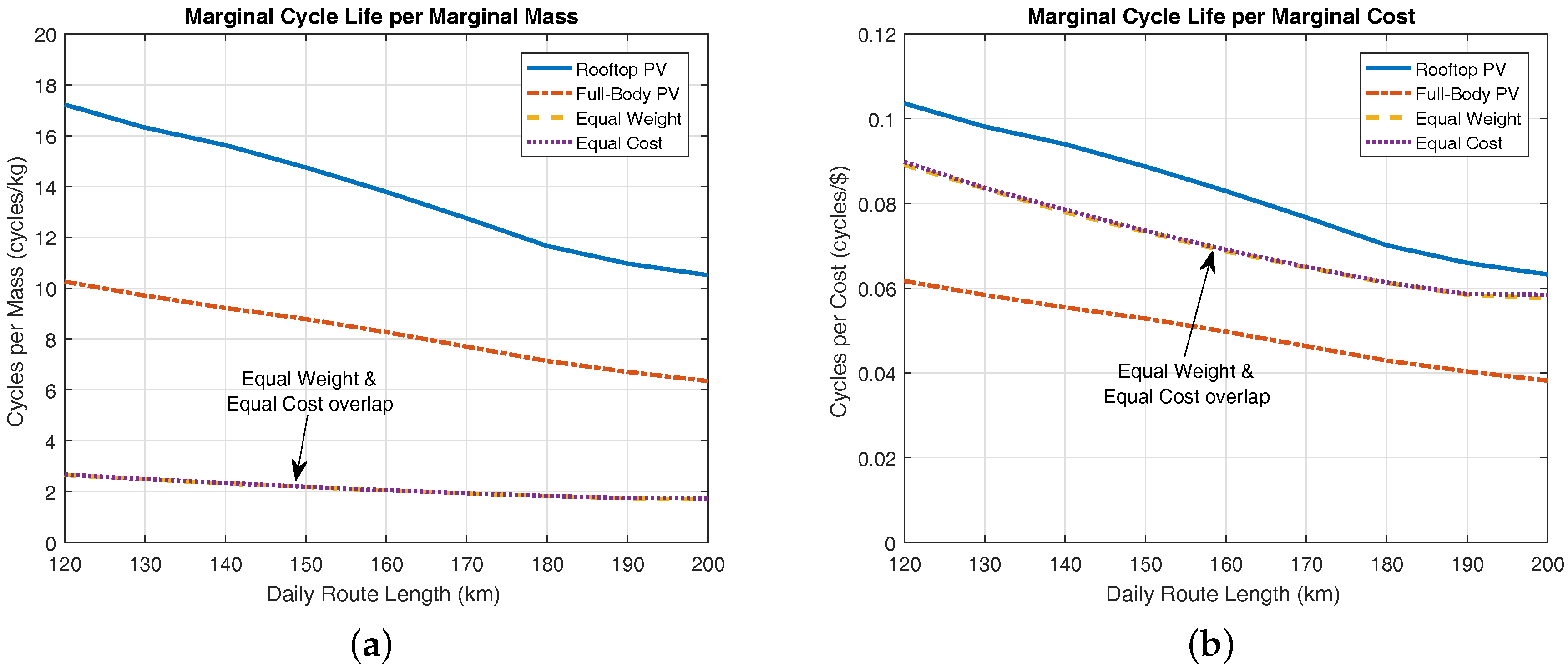
Figure 22a shows the marginal cycle life per marginal mass for each configuration and route length. Although the Full-Body PV configuration yielded the most additional cycles, the Rooftop PV configuration was a more effective use of mass. In general, adding PV modules to the bus was a more effective use of weight than increasing battery size.
Figure 22b shows the marginal cycle life per marginal cost for each configuration and route length. Due to the low amount of radiation that the side modules experienced, the Full-Body PV configuration was the most inefficient use of funds. Although the Equal Weight configuration added the fewest cycles, its marginal cycle life was achieved at very little expense. Both added-battery configurations outperformed the Full-Body PV configuration, but the Rooftop PV configuration was clearly the most cost-effective.
These relationships are visualized with the radar charts shown in Figure 23a–d. It should be noted that these plots use the inverse of marginal cost and marginal mass. This is done so that a large value corresponds to a desirable trait: large “per cost” indicates an inexpensive option, while large “per mass” indicates a low-weight option. The axes of these plots are scaled so that the largest marginal cycle life, inverse marginal cost, and inverse marginal mass across the four cases are all the same distance from the origin. Although the Rooftop PV and Equal Cost configurations had the same initial cost, the Rooftop PV configuration provided moderately longer cycle life and was a much more effective use of weight. The Full-Body PV provided the largest extension to battery life, but was neither as cost or weight effective as PV modules on the bus roof only. The Equal Weight configuration was both low-cost and low-weight, but provided little in the way of additional battery lifespan. Overall, the Rooftop PV configuration offered the best balance of extending battery cycle life while keeping weight and cost low.
Alternatively, one could define a non-dimensional cost or reward function to compare the four configurations with a single metric. For example, Equation (57) is a reward function that increases with larger cycle life improvements and decreases with larger costs at rates defined by the weighting parameters , , and , where is the average marginal cycle life, is the marginal mass, and is the marginal cost:
One could select , , and , which normalizes the three variables so that, among the four configurations, the reward due to the maximum mean marginal cycle life is equal to the combined penalty of the maximum marginal mass and maximum marginal cost. The resulting reward/penalty of each configuration for this function and weighting are shown in Figure 24. Once again, the Rooftop PV configuration strikes the best balance between added cycle life and added cost and weight. The higher weight lower marginal cycle life of the larger-battery configurations result in a net penalty rather than reward, indicating that OBPV is a better choice to extend battery lifespan. Of course, these results are heavily dependent on the choice of reward function.
A final metric for assessing the value of each configuration is the return on investment from an increase in cycle life. The nominal configuration was estimated to cost $118,580. Then, the cost per cycle of the nominal configuration can be estimated by dividing the estimated cost by the nominal configuration cycle life :
The value of the cycles added by each configuration can then be found by multiplying the nominal cost per cycle by the marginal cycle life of a given configuration:
The net profit or loss is found by subtracting the marginal cost of a given configuration:
Return on investment (ROI) is then found by normalizing by the marginal cost of that same configuration and expressing the result as a percent:
Here, indicates the break-even point, while indicates that the value of the added cycle life is twice the estimated cost of the configuration.
The ROI for each configuration and daily driving distance are shown in Figure 25. For all configurations, the ROI is greater with longer daily driving distances—or, rather, for routes where the battery is discharged to a greater depth. The Rooftop PV configuration is seen to provide a positive ROI for all route lengths, while the Full-Body PV configuration is a net loss until the daily driving distance reaches 160 km. The added-battery configurations are beneficial, but not to the extent of the Rooftop PV configuration.
5. Conclusions
This paper proposed modifying an electric bus to have OBPV power generation. PV modules mounted on both the vehicle roof and vehicle sides were considered. A modeling framework of an electric bus was developed so that the impact of the OBPV could be assessed for different locations, bus routes, and bus componentry. In particular, a method was developed to model the solar irradiance on a moving surface. Daily operation of an electric bus on a suburban bus route in Davis, CA, USA was simulated as a case study.
The results of the numerical experiment showed that, on average, the collected power could extend range by approximately 4.7 km per 100 km driven with rooftop panels and 8.9 km per 100 km driven with rooftop and side panels. However, high variance in the daily power collected meant that OBPV were not a robust means of range extension.
The PV modules could supply up to 8881 kWh of energy annually when mounted on both the roof and sides of the bus, or up to 4560 kWh of energy annually when mounted on the roof only. Although the side modules occupied approximately twice the area of the rooftop module, over the course of a year, they produced 5% less energy than the roof modules, indicating that side-mounted modules were not as effective but could still prove beneficial after all of the rooftop area has been exploited. The payback time for the roof-mounted panels was estimated to be six years, while the payback time of the side-mounted panels was estimated to be 13 years and three months. However, this payback time did not consider the value added by increasing battery cycle life.
The results were also used to assess the impact of OBPV on battery lifespan. For constant vehicle range, Rooftop PV modules could extend battery cycle life by up to 10%, while PV modules on both the roof and sides could extend it by up to 19%. Rooftop PV modules were shown to be both a more weight-effective and cost-effective means of increasing battery cycle life than expanding the size of the battery. Adding PV modules to both the roof and sides of the bus extended battery life the most and was more weight-effective than increasing battery size, but was the least cost-effective method. The additional lifespan added by the Rooftop PV was a positive return on investment, while the return on investment for a system with modules on both the roof and sides was negative unless the battery was discharged deeply each day.
Future work will include experimental validation of both the photovoltaics model and the battery aging model. In particular, the modeling assumptions for shading losses on a moving vehicle must be verified for the bus route under consideration.
Acknowledgments
This work was supported by Department of Mechanical and Aerospace Engineering, the University of California, Davis.
Author Contributions
Kevin R. Mallon, Francis Assadian, and Bo Fu conceived and designed the experiments; Kevin R. Mallon developed the bus model performed the numerical experiments; Kevin R. Mallon, Francis Assadian, and Bo Fu analyzed the data; and Kevin R. Mallon wrote the paper.
Conflicts of Interest
The authors declare no conflict of interest.
Abbreviations
| PV | Photovoltaics |
| OBPV | On-Board Photovoltaics |
| DC | Direct Current |
| AC | Alternating Current |
| OCV | Open-Circuit Voltage |
| SOC | State of Charge |
| DOD | Depth of Discharge |
| PM | Palmgren–Miner |
| CL | Cycle Life |
| TMY | Typical Meteorological Year |
| NREL | National Renewable Energy Lab |
| SPD | Surface Power Density |
| AD | Area Density |
| DNI | Direct Normal Irradiance |
| DHI | Diffuse Horizontal Irradiance |
| MPP | Maximum Power Point |
| SRC | Standard Reporting Conditions |
| NOCT | Nominal Operating Cell Temperature |
| OCTA | Orange County Transit Authority |
| ROI | Return On Investment |
References
- Abdel-Rahman, A.A. On the emissions from internal-combustion engines: A review. Int. J. Energy Res. 1998, 22, 483–513. [Google Scholar] [CrossRef]
- Yanowitz, J.; McCormick, R.L.; Graboski, M.S. In-Use Emissions from Heavy-Duty Diesel Vehicles. Environ. Sci. Technol. 2000, 34, 729–740. [Google Scholar] [CrossRef]
- Lee, T.K.; Filipi, Z. Impact of Model-Based Lithium-Ion Battery Control Strategy on Battery Sizing and Fuel Economy in Heavy-Duty HEVs. SAE Int. J. Commer. Veh. 2011, 4, 198–209. [Google Scholar] [CrossRef]
- Geca, M.; Wendeker, M.; Grabowski, L. A City Bus Electrification Supported by the Photovoltaic Power Modules; SAE Technical Paper; SAE International: Birmingham, UK, 2014. [Google Scholar]
- Abdel Dayem, A.M. Set-up and performance investigation of an innovative solar vehicle. J. Renew. Sustain. Energy 2012, 4, 033109:1–033109:18. [Google Scholar] [CrossRef]
- Kimura, K.; Kudo, Y.; Sato, A. Techno-Economic Analysis of Solar Hybrid Vehicles Part 1: Analysis of Solar Hybrid Vehicle Potential Considering Well -to-Wheel GHG Emissions; SAE Technical Paper; SAE International: Birmingham, UK, 2016. [Google Scholar]
- Hara, T.; Shiga, T.; Kimura, K.; Sato, A. Techno-Economic Analysis of Solar Hybrid Vehicles Part 2: Comparative Analysis of Economic, Environmental, and Usability Benefits; SAE Technical Paper; SAE International: Birmingham, UK, 2016. [Google Scholar]
- Abdelhamid, M. A Comprehensive Assessment Methodology Based on Life Cylce Analysis for On-Board Photovoltaic Solar Modeules in Vehicles. Ph.D. Thesis, Clemson University, Clemson, SC, USA, 2014. [Google Scholar]
- Giannouli, M.; Yianoulis, P. Study on the incorporation of photovoltaic systems as an auxiliary power source for hybrid and electric vehicles. Sol. Energy 2012, 86, 441–451. [Google Scholar] [CrossRef]
- Rizzo, G. Automotive Applications of Solar Energy. IFAC Proc. Vol. 2010, 43, 174–185. [Google Scholar] [CrossRef]
- Almonacid, G.; Muñoz, F.J.; de la Casa, J.; Aguilar, J.D. Integration of PV systems on health emergency vehicles. The FIVE project. Prog. Photovolt. Res. Appl. 2004, 12, 609–621. [Google Scholar] [CrossRef]
- Bahaj, A.S.; James, P.A.B. Economics of solar powered refrigeration transport applications. In Proceedings of the Conference Record of the Twenty-Ninth IEEE Photovoltaic Specialists Conference, New Orleans, LA, USA, 19–24 May 2002; IEEE: New Orleans, LA, USA, 2002; pp. 1561–1564. [Google Scholar]
- Kronthaler, L.; Maturi, L.; Moser, D.; Alberti, L. Vehicle-integrated Photovoltaic (ViPV) systems: Energy production, Diesel Equivalent, Payback Time; an assessment screening for trucks and busses. In Proceedings of the 2014 Ninth International Conference on Ecological Vehicles and Renewable Energies (EVER), Monte-Carlo, Monaco, 25–27 March 2014; pp. 1–8. [Google Scholar]
- Xue, J. Assessment of agricultural electric vehicles based on photovoltaics in China. J. Renew. Sustain. Energy 2013, 5, 6745–6759. [Google Scholar] [CrossRef]
- Azwan, M.B.; Norasikin, A.L.; Sopian, K.; Abd Rahim, S.; Norman, K.; Ramdhan, K.; Solah, D. Assessment of electric vehicle and photovoltaic integration for oil palm mechanisation practise. J. Clean. Prod. 2017, 140 Pt 3, 1365–1375. [Google Scholar] [CrossRef]
- Assadian, F.; Mallon, K.R.; Fu, B. The Impact of Vehicle-Integrated Photovoltaics on Heavy-Duty Electric Vehicle Battery Cost and Lifespan; SAE Technical Paper; SAE International: Birmingham, UK, 2016. [Google Scholar]
- Mohan, G.; Assadian, F.; Longo, S. Comparative analysis of forward-facing models vs backwardfacing models in powertrain component sizing. In Proceedings of the IET Hybrid and Electric Vehicles Conference 2013 (HEVC 2013), London, UK, 6–7 November 2013; pp. 1–6. [Google Scholar]
- Guzzella, L.; Sciarretta, A. Vehicle Propulsion Systems, 3rd ed.; Springer: Berlin/Heidelberg, Germany, 2013. [Google Scholar]
- Zeng, X.; Yang, N.; Wang, J.; Song, D.; Zhang, N.; Shang, M.; Liu, J. Predictive-model-based dynamic coordination control strategy for power-split hybrid electric bus. Mech. Syst. Signal Process. 2015, 60–61, 785–798. [Google Scholar] [CrossRef]
- Sangtarash, F.; Esfahanian, V.; Nehzati, H.; Haddadi, S.; Bavanpour, M.A.; Haghpanah, B. Effect of Different Regenerative Braking Strategies on Braking Performance and Fuel Economy in a Hybrid Electric Bus Employing CRUISE Vehicle Simulation. SAE Int. J. Fuels Lubr. 2008, 1, 828–837. [Google Scholar] [CrossRef]
- Wang, B.; Luo, Y.; Zhang, J. Simulation of city bus performance based on actual urban driving cycle in China. Int. J. Automot. Technol. 2008, 9, 501–507. [Google Scholar] [CrossRef]
- Proterra. Catalyst 40-Foot Transit Vehicle. Available online: https://www.proterra.com/products/catalyst-40ft/ (accessed on 10 March 2017).
- Lesster, L.E.; Lindberg, F.A.; Young, R.M.; Hall, W.B. An Induction Motor Power Train for EVs—The Right Power at the Right Price. In Advanced Components for Electric and Hybrid Electric Vehicles: Workshop Proceedings; Stricklett, K.L., Ed.; National Institute of Standards and Technology: Gaithersburg, MD, USA, 1993; pp. 170–173. [Google Scholar]
- He, H.; Xiong, R.; Fan, J. Evaluation of Lithium-Ion Battery Equivalent Circuit Models for State of Charge Estimation by an Experimental Approach. Energies 2011, 4, 582–598. [Google Scholar] [CrossRef]
- Valence Technology, Inc. Lithium Iron Magnesium Phosphate 26650 Power Cell. 2016. Available online: https://www.valence.com/products/cells/26650-power-cells/ (accessed on 10 March 2017).
- Saw, L.H.; Somasundaram, K.; Ye, Y.; Tay, A.A.O. Electro-thermal analysis of Lithium Iron Phosphate battery for electric vehicles. J. Power Sources 2014, 249, 231–238. [Google Scholar] [CrossRef]
- Williamson, S.S. Energy Management Strategies for Electric and Plug-In Hybrid Electric Vehicles; Springer: New York, NY, USA, 2013. [Google Scholar]
- Valence Technology, Inc. Valence Module Range. Available online: https://www.valence.com/wp-content/uploads/2016/11/Valence-Module-Range-113016.pdf (accessed on 10 March 2017).
- Nelson, R.F. Power requirements for batteries in hybrid electric vehicles. J. Power Sources 2000, 91, 2–26. [Google Scholar] [CrossRef]
- DiOrio, N.; Dobos, A.; Janzou, S.; Nelson, A.; Lundstrom, B. Technoeconomic Modeling of Battery Energy Storage in SAM; Technical Report NREL/TP-6A20–64641; National Renewable Energy Laboratory (NREL): Golden, CO, USA, 2015. [Google Scholar]
- Ramadesigan, V.; Northrop, P.W.C.; De, S.; Santhanagopalan, S.; Braatz, R.D.; Subramanian, V.R. Modeling and Simulation of Lithium-Ion Batteries from a Systems Engineering Perspective. J. Electrochem. Soc. 2012, 159, R31–R45. [Google Scholar] [CrossRef]
- Pelletier, S.; Jabali, O.; Laporte, G.; Veneroni, M. Battery degradation and behaviour for electric vehicles: Review and numerical analyses of several models. Transp. Res. Part B Methodol. 2017. [Google Scholar] [CrossRef]
- Safari, M.; Morcrette, M.; Teyssot, A.; Delacourt, C. Life-Prediction Methods for Lithium-Ion Batteries Derived from a Fatigue Approach I. Introduction: Capacity-Loss Prediction Based on Damage Accumulation. J. Electrochem. Soc. 2010, 157, A713–A720. [Google Scholar] [CrossRef]
- Valence Technology, Inc. Long Cycle Life Lithium Iron Magnesium Phosphate Battery. 2014. Available online: https://www.valence.com/why-valence/long-lifecycle/ (accessed on 10 March 2017).
- Zhou, C.; Qian, K.; Allan, M.; Zhou, W. Modeling of the Cost of EV Battery Wear Due to V2G Application in Power Systems. IEEE Trans. Energy Convers. 2011, 26, 1041–1050. [Google Scholar] [CrossRef]
- Marano, V.; Onori, S.; Guezennec, Y.; Rizzoni, G.; Madella, N. Lithium-ion batteries life estimation for plug-in hybrid electric vehicles. In Proceedings of the 2009 IEEE Vehicle Power and Propulsion Conference, Dearborn, MI, USA, 7–11 September 2009; pp. 536–543. [Google Scholar]
- Millner, A. Modeling Lithium Ion battery degradation in electric vehicles. In Proceedings of the 2010 IEEE Conference on Innovative Technologies for an Efficient and Reliable Electricity Supply, Waltham, MA, USA, 27–29 September 2010; pp. 349–356. [Google Scholar]
- Ma, C.C.Y.; Iqbal, M. Statistical comparison of solar radiation correlations Monthly average global and diffuse radiation on horizontal surfaces. Sol. Energy 1984, 33, 143–148. [Google Scholar] [CrossRef]
- Tracy, C.R.; Hammond, K.A.; Lechleitner, R.A.; Smith, W.J.; Thompson, D.B.; Whicker, A.D.; Williamson, S.C. Estimating clear-day solar radiation: An evaluation of three models. J. Therm. Biol. 1983, 8, 247–251. [Google Scholar] [CrossRef]
- Wilcox, S.; Marion, W. Users Manual for TMY3 Data Sets; Technical Report NREL/TP-581-43156; National Renewable Energy Laboratory: Golden, CO, USA, 2008.
- Arsie, I.; Marotta, M.; Pianese, C.; Rizzo, G.; Sorrentino, M. Optimal Design of a Hybrid Electric Car with Solar Cells. In Proceedings of the 1st AUTOCOM Workshop on Preventive and Active Safety Systems for Road Vehicles, Istanbul, Turkey, 19–20 September 2005. [Google Scholar]
- Emery, K. Measurement and Characterization of Solar Cells and Modules. In Handbook of Photovoltaic Science and Engineering, 2nd ed.; Luque, A., Hegedus, S., Eds.; John Wiley & Sons, Ltd.: Chichester, UK, 2011; pp. 797–840. [Google Scholar]
- HighFlex Solar, Inc. HF315-6-36b. Available online: http://www.highflexsolar.com/docs/HighFlexSolar_HF315-6-36b_Datasheet_v1.0.pdf (accessed on 10 March 2017).
- Reda, I.; Andreas, A. Solar position algorithm for solar radiation applications. Sol. Energy 2004, 76, 577–589. [Google Scholar] [CrossRef]
- Loutzenhiser, P.G.; Manz, H.; Felsmann, C.; Strachan, P.A.; Frank, T.; Maxwell, G.M. Empirical validation of models to compute solar irradiance on inclined surfaces for building energy simulation. Sol. Energy 2007, 81, 254–267. [Google Scholar] [CrossRef]
- Villalva, M.G.; Gazoli, J.R.; Filho, E.R. Comprehensive Approach to Modeling and Simulation of Photovoltaic Arrays. IEEE Trans. Power Electron. 2009, 24, 1198–1208. [Google Scholar] [CrossRef]
- Jain, A.; Kapoor, A. Exact analytical solutions of the parameters of real solar cells using Lambert W-function. Sol. Energy Mater. Sol. Cells 2004, 81, 269–277. [Google Scholar] [CrossRef]
- Esram, T.; Chapman, P.L. Comparison of Photovoltaic Array Maximum Power Point Tracking Techniques. IEEE Trans. Energy Convers. 2007, 22, 439–449. [Google Scholar] [CrossRef]
- Bidram, A.; Davoudi, A.; Balog, R.S. Control and Circuit Techniques to Mitigate Partial Shading Effects in Photovoltaic Arrays. IEEE J. Photovolt. 2012, 2, 532–546. [Google Scholar] [CrossRef]
- Emery, K.; Burdick, J.; Caiyem, Y.; Dunlavy, D.; Field, H.; Kroposki, B.; Moriarty, T.; Ottoson, L.; Rummel, S.; Strand, T.; et al. Temperature dependence of photovoltaic cells, modules and systems. In Proceedings of the Conference Record of the Twenty Fifth IEEE Photovoltaic Specialists Conference, Washington, DC, USA, 13–17 May 1996; pp. 1275–1278. [Google Scholar]
- Muller, M. Measuring and Modeling Nominal Operating Cell Temperature (NOCT). Proceedings of PV Performance Modeling Workshop, Albuquerque, NM, USA, 22–23 September 2010. [Google Scholar]
- McCrone, A.; Moslener, U.; d’Estais, F.; Usher, E.; Grüning, C. Global Trends in Renewable Energy Investment 2016; FS-UNEP Collaborating Centre for Climate & Sustainable Energy Finance: Frankfurt am Main, Germany, 2016. [Google Scholar]
- Kahn, S.; Shiao, M.J.; Honeyman, C.; Perea, A.; Jones, J.; Smith, C.; Gallagher, B.; Moskowitz, S.; Baca, J.; Rumery, S.; et al. Solar Market Insight Report 2016 Q2; Solar Energy Industries Association: Washington, DC, USA, 2016. [Google Scholar]
- National Renewable Energy Laboratory. Dynamic Maps, GIS Data, and Analysis Tools—Solar Maps. Available online: http://www.nrel.gov/gis/solar.html (accessed on 10 March 2017).
- National Renewable Energy Laboratory. National Solar Radiation Data Base, and Analysis Tools—Solar Maps. Available online: http://rredc.nrel.gov/solar/old_data/nsrdb/1991-2005/tmy3/by_state_and_city.html (accessed on 23 May 2017).
- California Air Resource Board. Public Transit Bus Fleet Rule and Emission Standards for New Urban Buses. Available online: https://www.arb.ca.gov/regact/bus02/bus02.htm (accessed on 10 March 2017).
- Pacific Gas and Electric Company. Electric Rates. Available online: https://www.pge.com/tariffs/electric.shtml (accessed on 15 April 2017).
Figure 1.
Vehicle model diagram.

Figure 2.
Diagram of battery, photovoltaic (PV) panel, and motor connections.
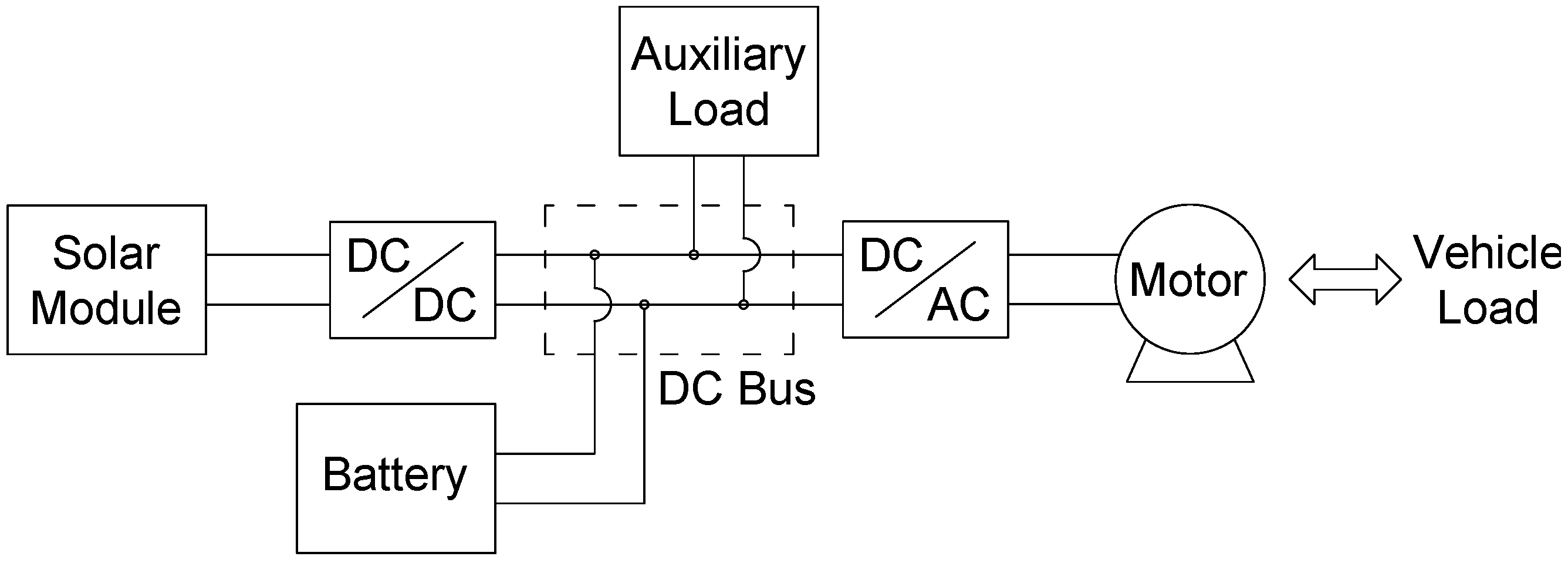
Figure 3.
Battery cell and battery pack equivalent circuit.
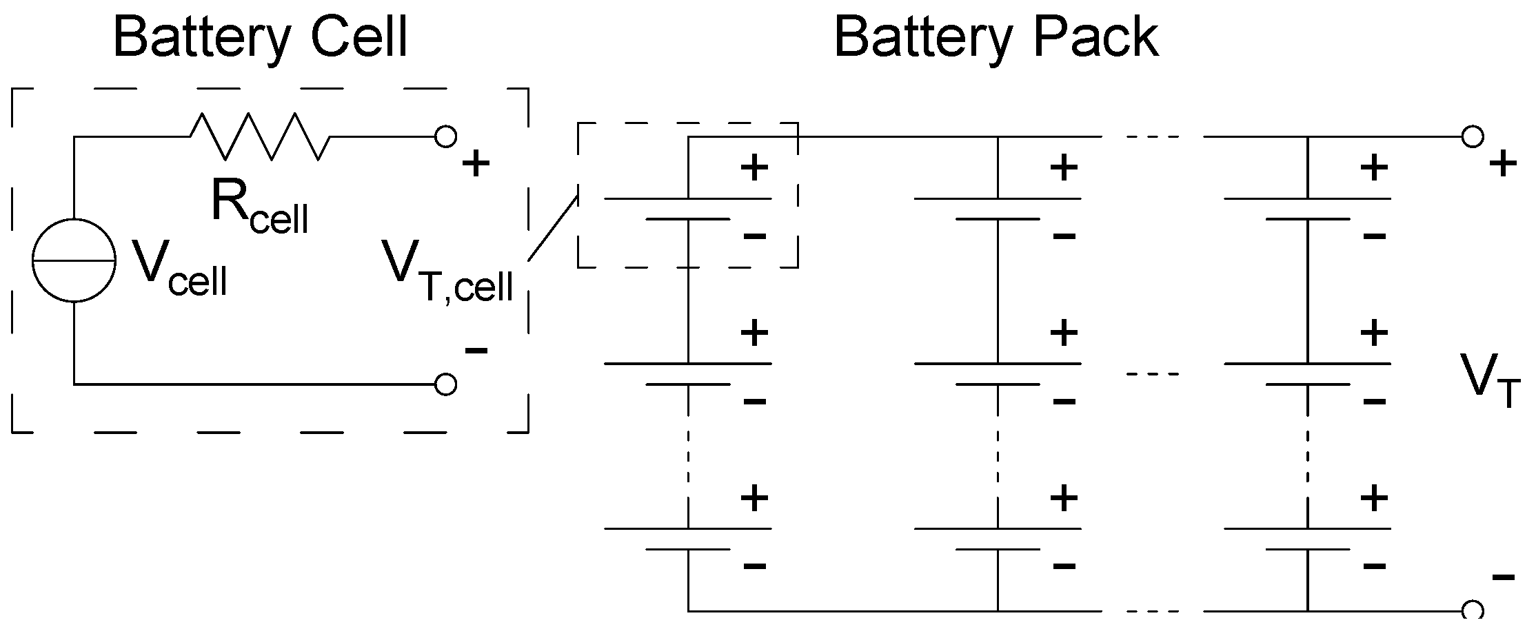
Figure 4.
Depth of discharge versus cycle life of the lithium-ion battery.
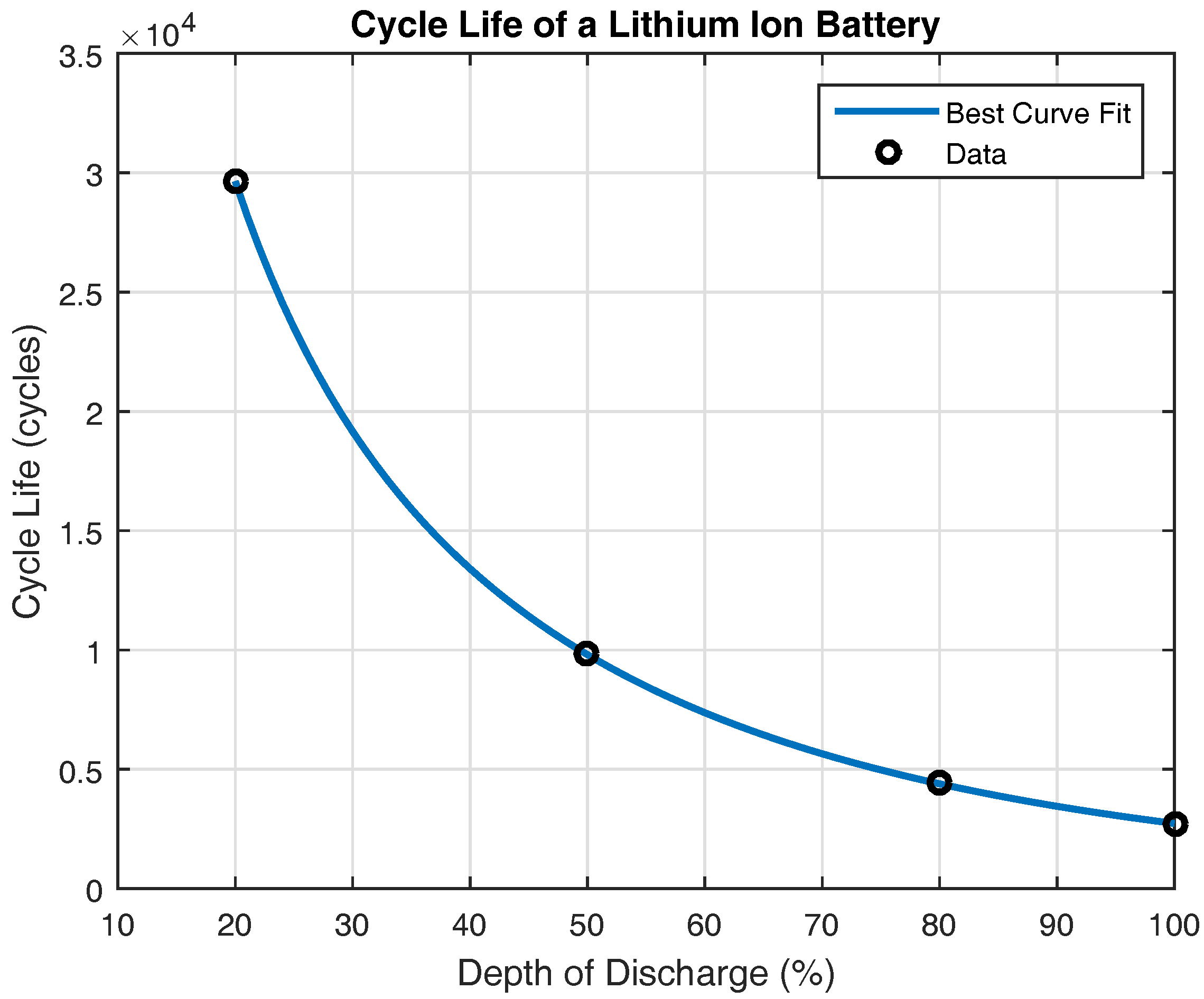
Figure 5.
Types of solar radiation.

Figure 6.
Direct radiation.

Figure 7.
Global coordinate system.

Figure 8.
Bus coordinate system.

Figure 9.
(a) Heading rotation; and (b) pitch rotation.
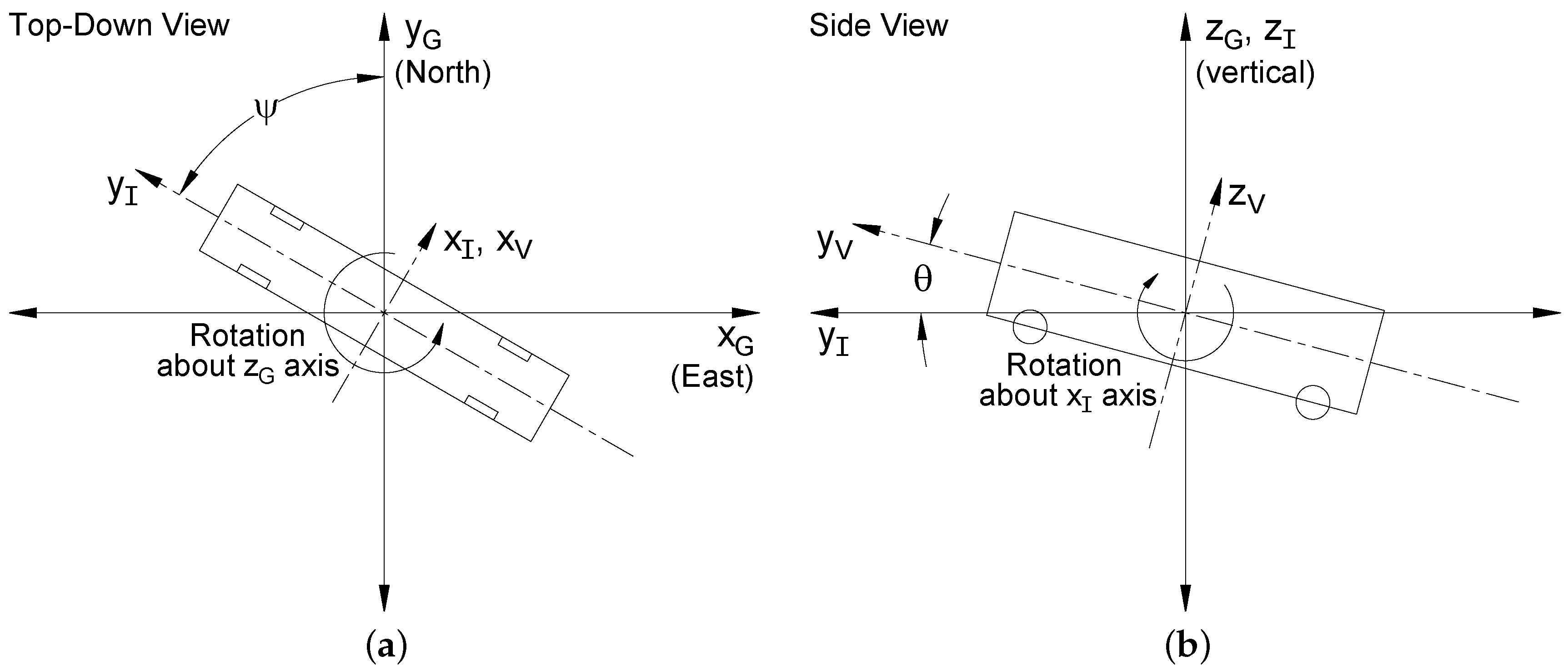
Figure 10.
Tilt angle of Rooftop and Back PV modules.
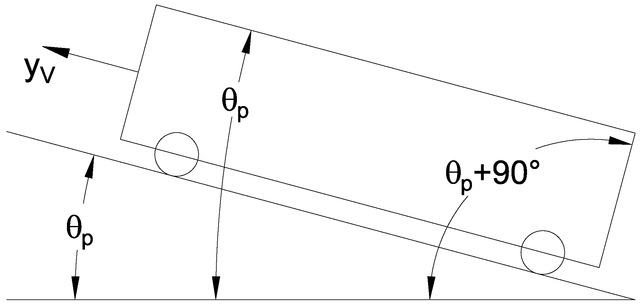
Figure 11.
PV module equivalent circuit.
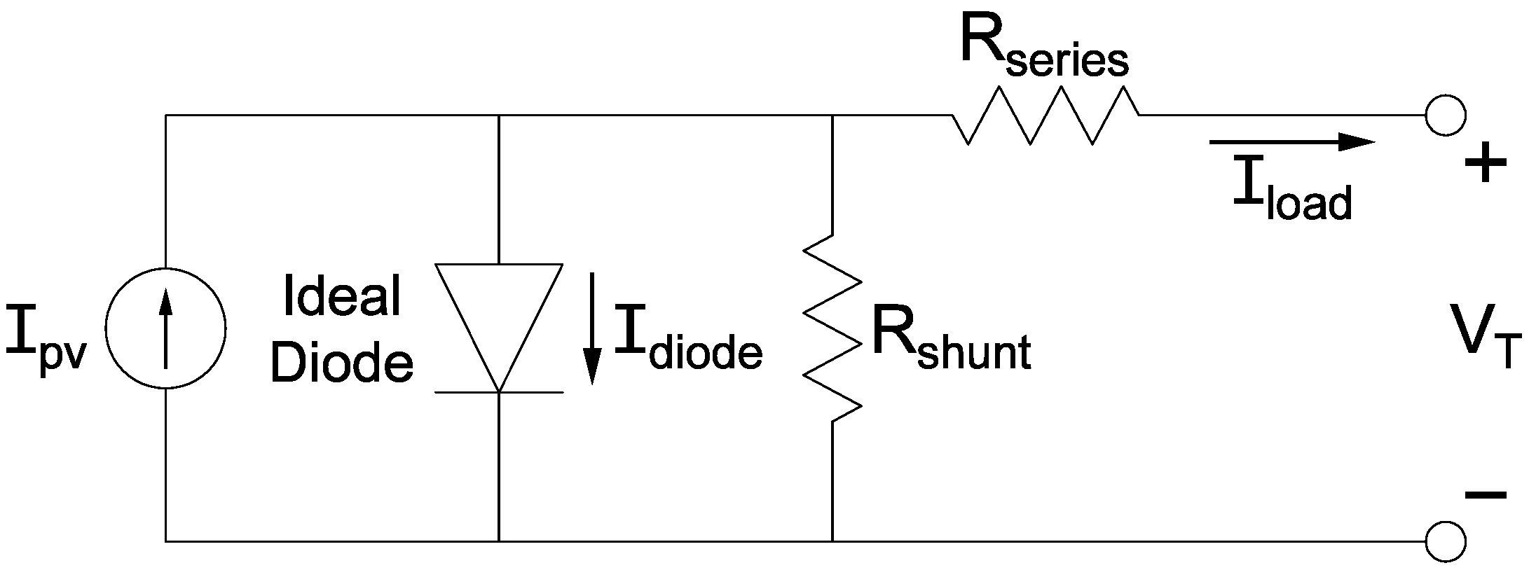
Figure 12.
Typical PV module I–V curve.

Figure 13.
Orange county transit authority (OCTA) suburban bus drive cycle.

Figure 14.
Davis Unitrans O-Route.
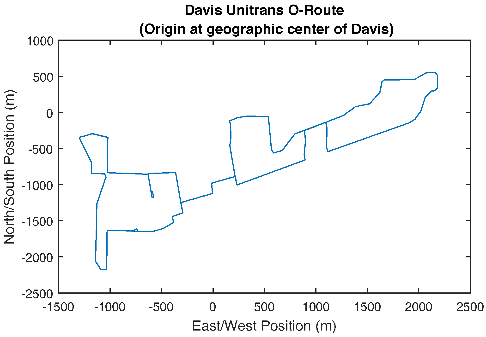
Figure 15.
Simulated bus energy usage per configuration and time of year.

Figure 16.
Histogram of range extension provided by on-board PV (OBPV).

Figure 17.
Intensities of solar radiation reaching the bus: (a) on a typical clear day; and (b) over the course of each month.
Figure 17.
Intensities of solar radiation reaching the bus: (a) on a typical clear day; and (b) over the course of each month.
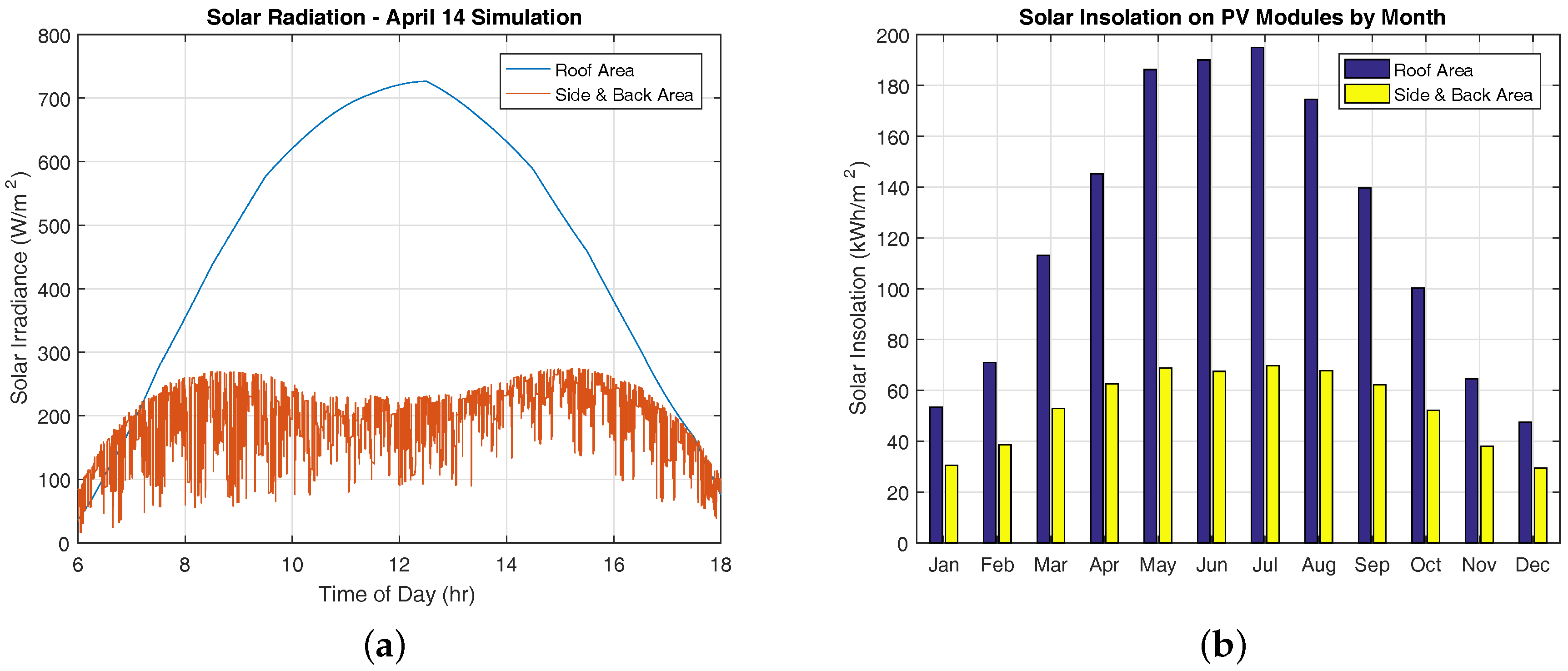
Figure 18.
Monthly electric energy collected from (a) roof and side PV modules; and (b) right, left, and back PV modules.
Figure 18.
Monthly electric energy collected from (a) roof and side PV modules; and (b) right, left, and back PV modules.

Figure 19.
PV contribution towards total annual energy consumption.

Figure 20.
Battery capacity fade on the 160 km bus route.
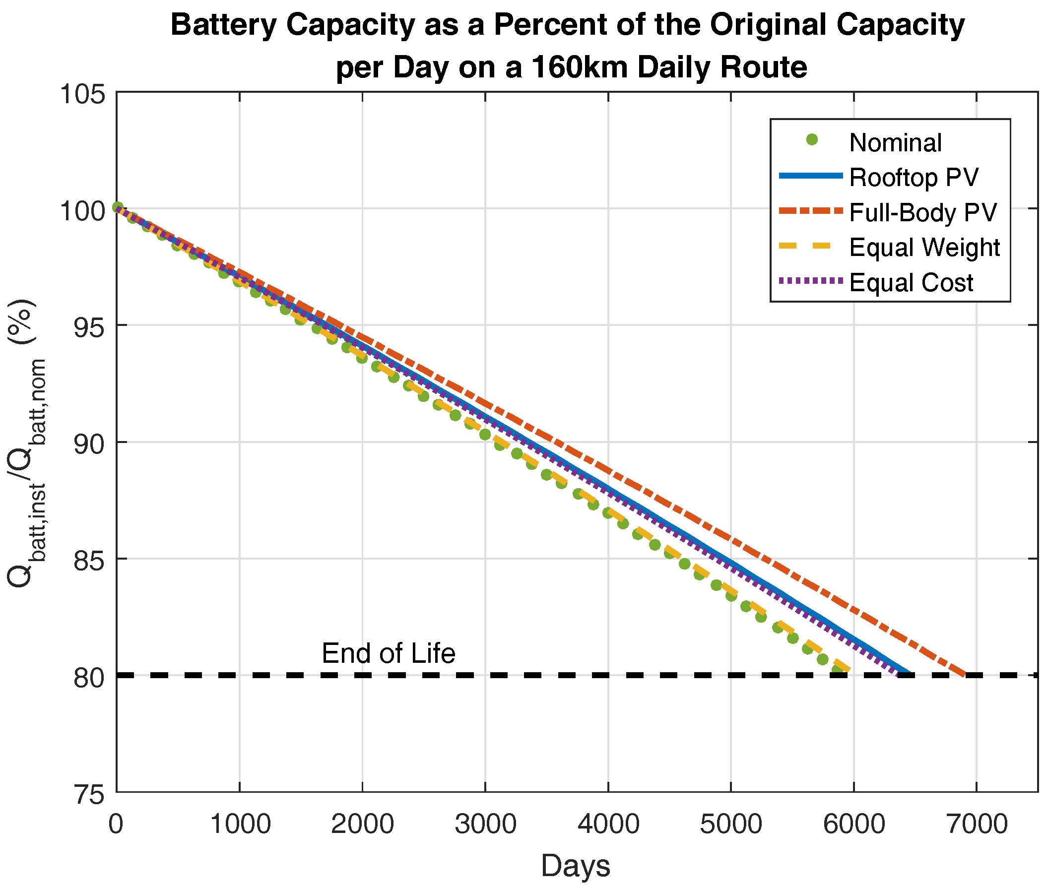
Figure 21.
(a) Battery cycle life; and (b) increase in battery cycle per configuration.
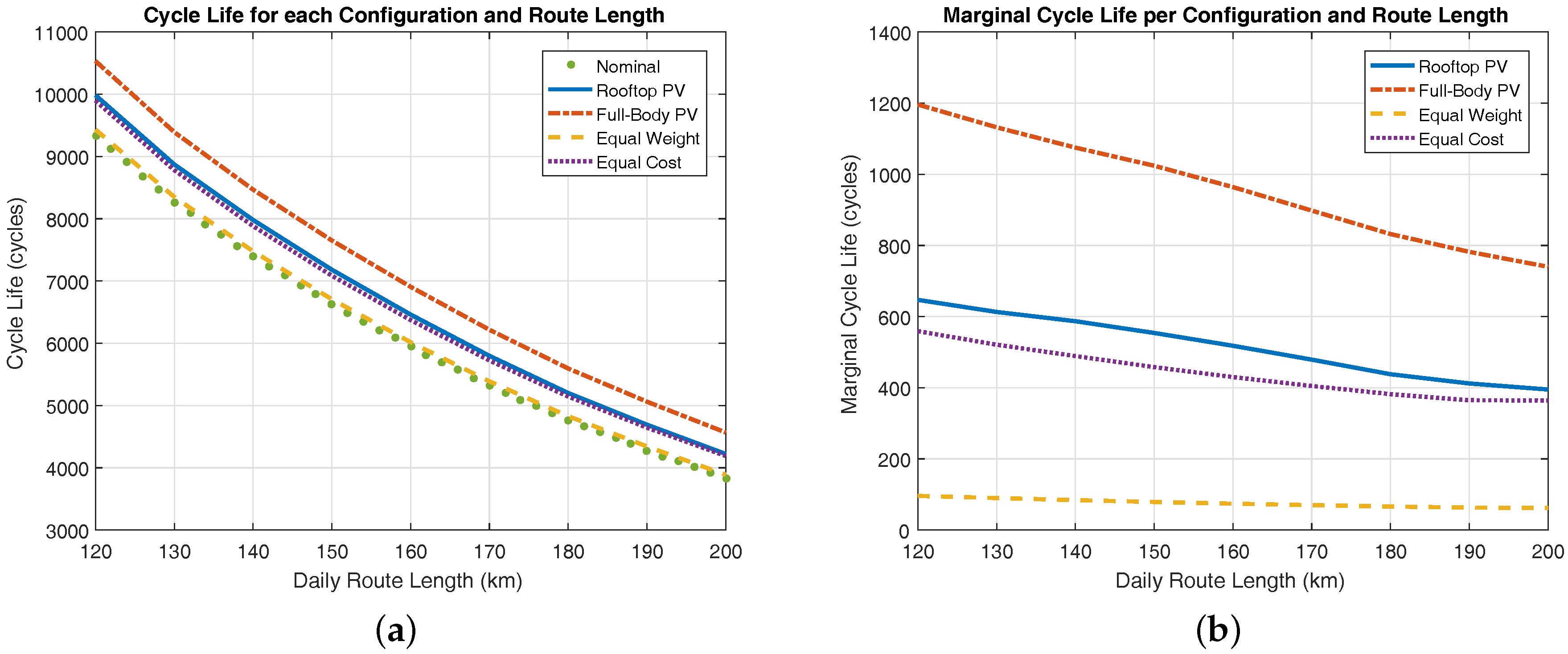
Figure 22.
Marginal cycle life (a) per marginal mass; and (b) per marginal cost.

Figure 23.
Radar plots of the performance metrics for (a) rooftop PV; (b) full-body PV; (c) equal weight; and (d) equal cost.
Figure 23.
Radar plots of the performance metrics for (a) rooftop PV; (b) full-body PV; (c) equal weight; and (d) equal cost.

Figure 24.
Evaluation of each configuration using a reward function.

Figure 25.
Return on investment of OBPV and increased battery size.


Table 1.
Vehicle model parameters.
| Parameter | Variable | Value |
|---|---|---|
| Vehicle Mass | 15,500 kg | |
| Frontal Area | 8.02 m | |
| Aerodynamic Drag Coefficient | 0.55 | |
| Rolling Resistance Coefficient | 0.008 | |
| Wheel Inertia | 20.52 kg-m | |
| Motor Inertia | 0.277 kg-m | |
| Wheel Radius | 0.48 m | |
| Final Drive Ratio | 5.5:1 | |
| Gearbox Ratio | 5:1 | |
| Transmission Efficiency | 96% |
Table 2.
Battery model parameters.
| Parameter | Variable | Value |
|---|---|---|
| Open-Circuit Voltage per Cell | 2.0 to 3.4 V | |
| Rated Energy Capacity per Cell | 8 Wh | |
| Rated Charge Capacity per Cell | 2.5 Ah | |
| Battery Cell Equivalent Resistance | 6 m | |
| Battery Cells in Parallel | 385 cells | |
| Parallel Sets in Series | 110 sets | |
| Battery Weight per Cell | 94 g |
Table 3.
Photovoltaic (PV) model parameters.
| Parameter | Variable | Value |
|---|---|---|
| Vehicle Roof Area | 33.2 m | |
| Vehicle Side Area | 44.1 m | |
| Vehicle Back Area | 8.81 m | |
| Surface Power Density | 165 W/m | |
| Area Density | 1.89 kg/m | |
| Peak Power Temperature Coefficient | −0.43%/C |
Table 4.
Bus configurations.
| Configuration | PV Modules | Battery Size |
|---|---|---|
| Nominal | None | 338.8 kWh |
| Rooftop PV | Top Only | 338.8 kWh |
| Full-Body PV | Top, Sides, and Back | 338.8 kWh |
| Equal Weight | None | 341.9 kWh |
| Equal Cost | None | 356.6 kWh |
Table 5.
Marginal mass and cost of bus configurations.
| Configuration | Marginal Mass | Marginal Cost |
|---|---|---|
| Rooftop PV | 37.6 kg | $6247 |
| Full-Body PV | 116.6 kg | $19,386 |
| Equal Weight | 36.2 kg | $1220 |
| Equal Cost | 209.3 kg | $6227 |
© 2017 by the authors. Licensee MDPI, Basel, Switzerland. This article is an open access article distributed under the terms and conditions of the Creative Commons Attribution (CC BY) license (http://creativecommons.org/licenses/by/4.0/).
Share and Cite
MDPI and ACS Style
Mallon, K.R.; Assadian, F.; Fu, B. Analysis of On-Board Photovoltaics for a Battery Electric Bus and Their Impact on Battery Lifespan. Energies 2017, 10, 943. https://doi.org/10.3390/en10070943
AMA Style
Mallon KR, Assadian F, Fu B. Analysis of On-Board Photovoltaics for a Battery Electric Bus and Their Impact on Battery Lifespan. Energies. 2017; 10(7):943. https://doi.org/10.3390/en10070943
Chicago/Turabian StyleMallon, Kevin R., Francis Assadian, and Bo Fu. 2017. "Analysis of On-Board Photovoltaics for a Battery Electric Bus and Their Impact on Battery Lifespan" Energies 10, no. 7: 943. https://doi.org/10.3390/en10070943
Note that from the first issue of 2016, this journal uses article numbers instead of page numbers. See further details here.