Optimizing the Weather Research and Forecasting (WRF) Model for Mapping the Near-Surface Wind Resources over the Southernmost Caribbean Islands of Trinidad and Tobago


Abstract
:1. Introduction
2. Area of Interest, Method and Data
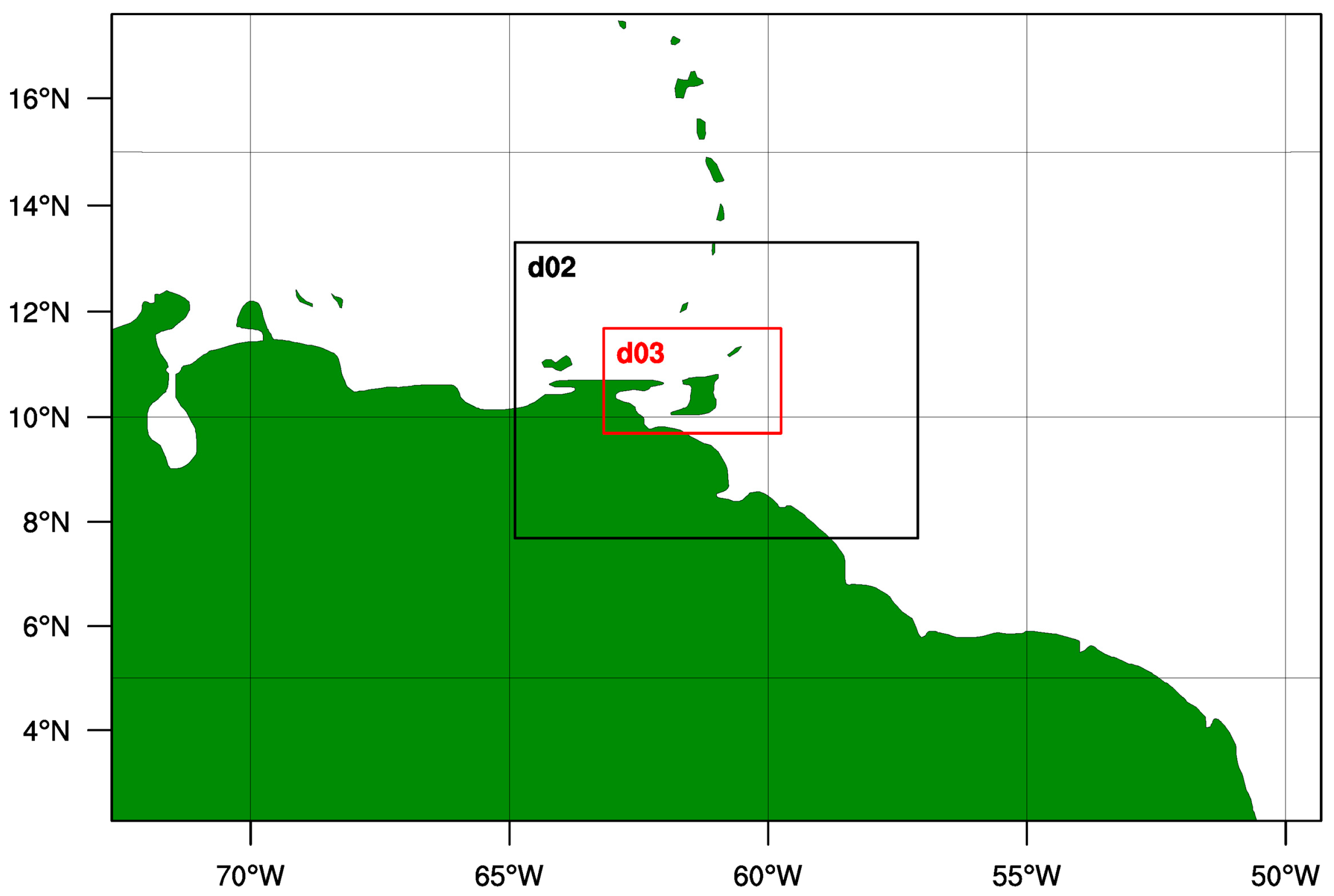
2.1. Area of Interest
2.2. Overview of Method and Data
2.2.1. Reanalysis Data for NWP Model Initialization
2.2.2. In-Situ Data and Error Metrics
2.2.3. Spin-Up Period
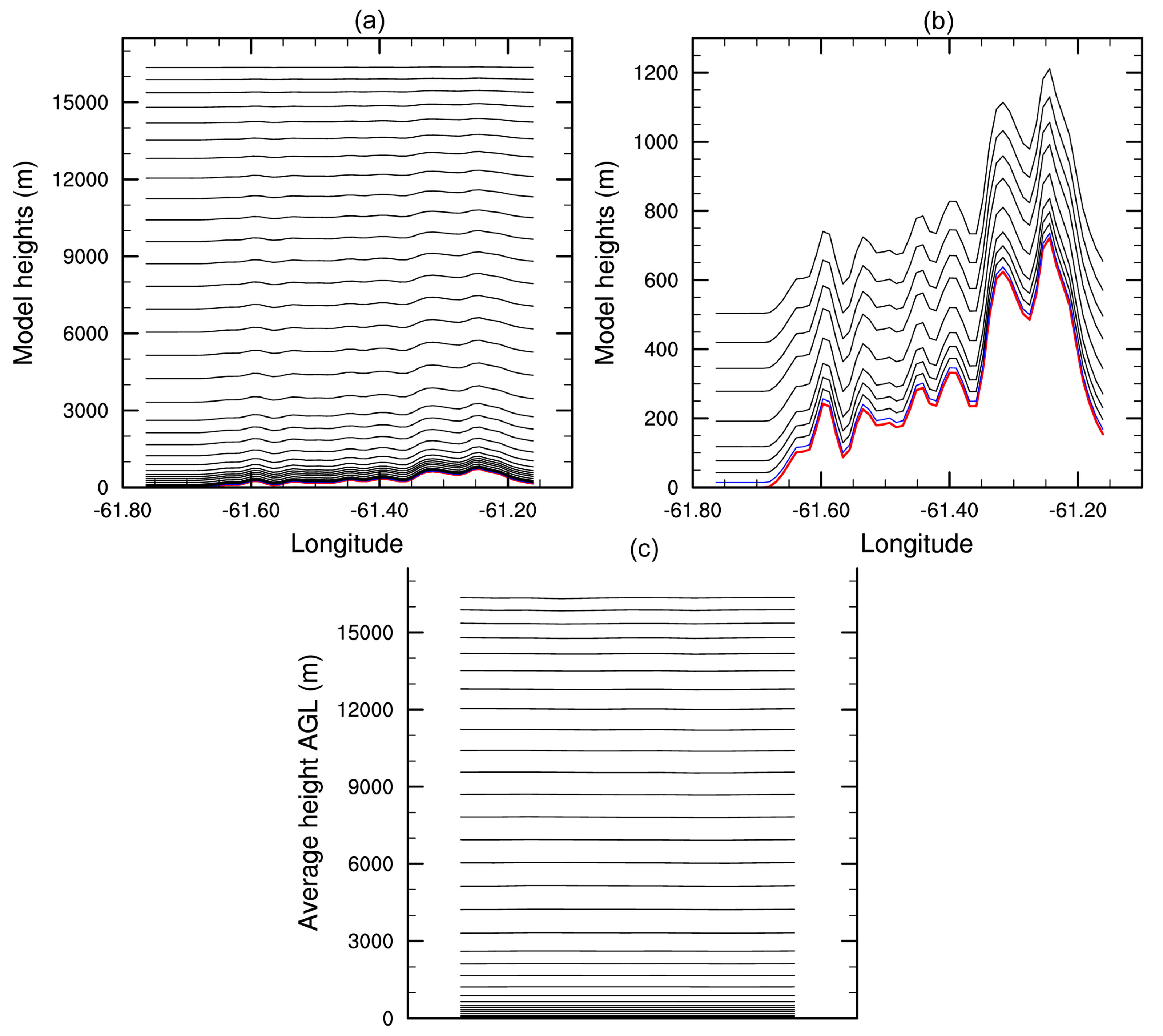
2.2.4. Initial Configuration for the Weather Research and Forecasting (WRF) Model
2.2.5. Planetary Boundary Layer (PBL) Schemes
3. Results
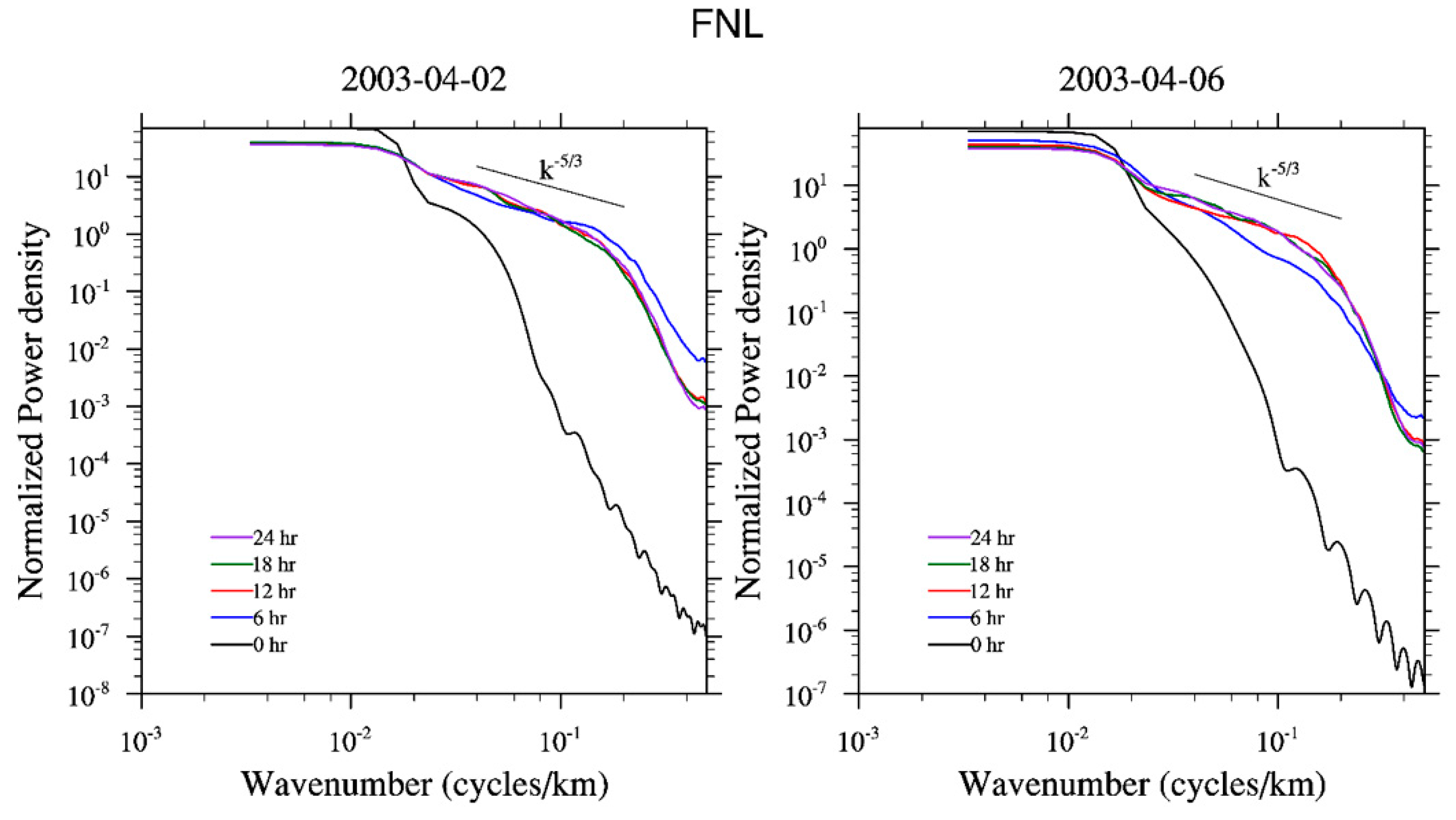
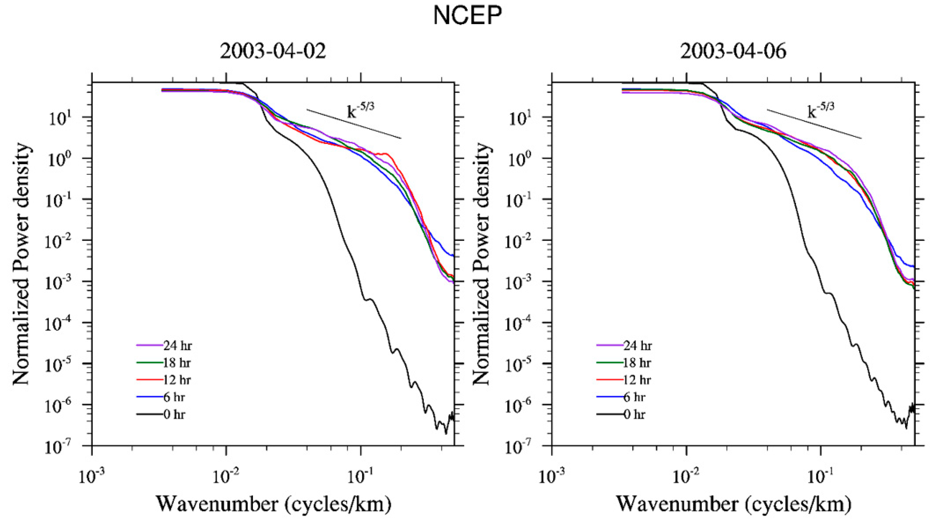
3.1. Spin-Up Period
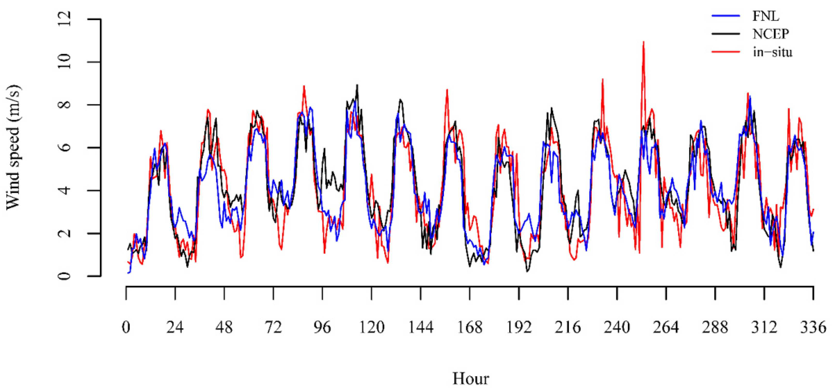
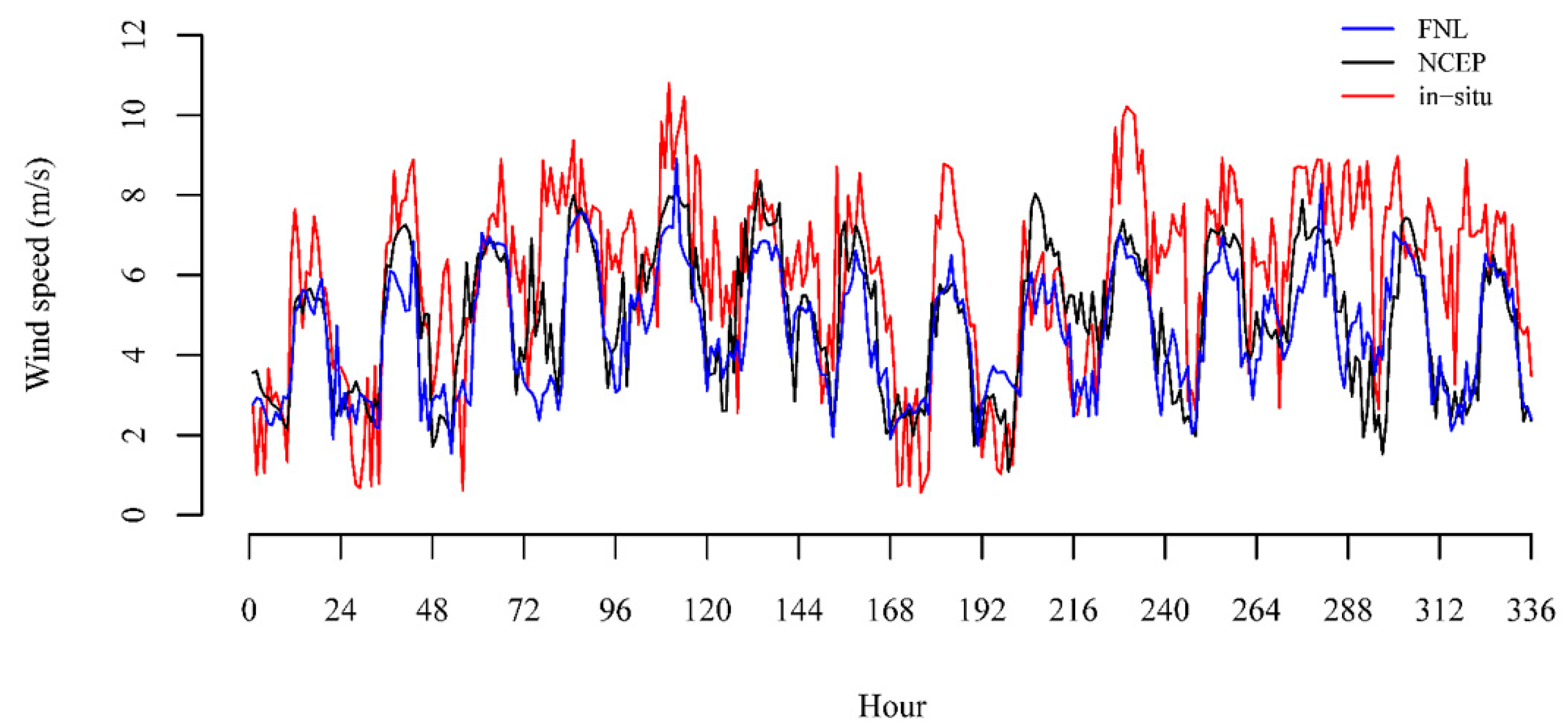
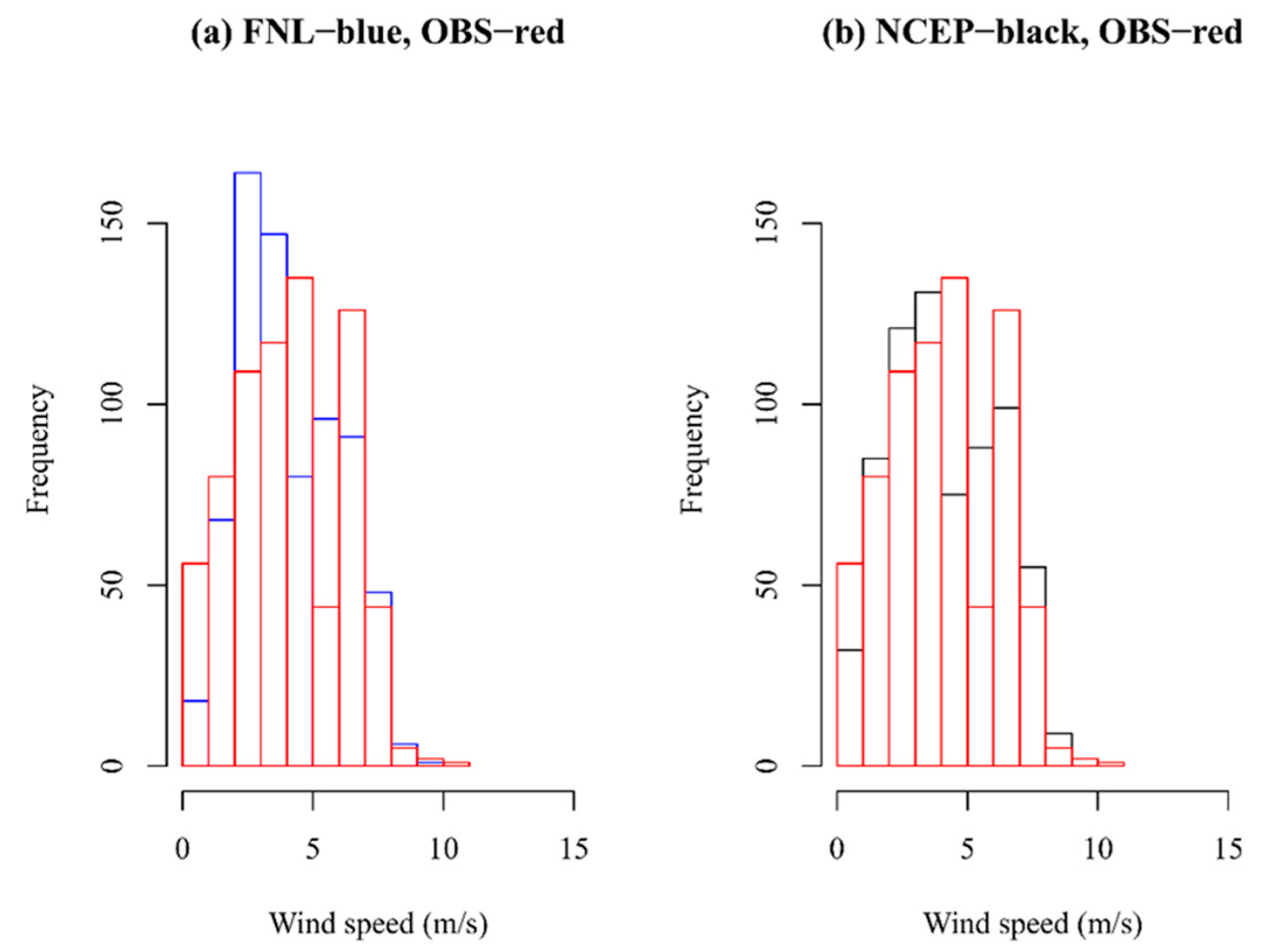
3.2. FNL vs NCEP As Initial and Boundary Conditions
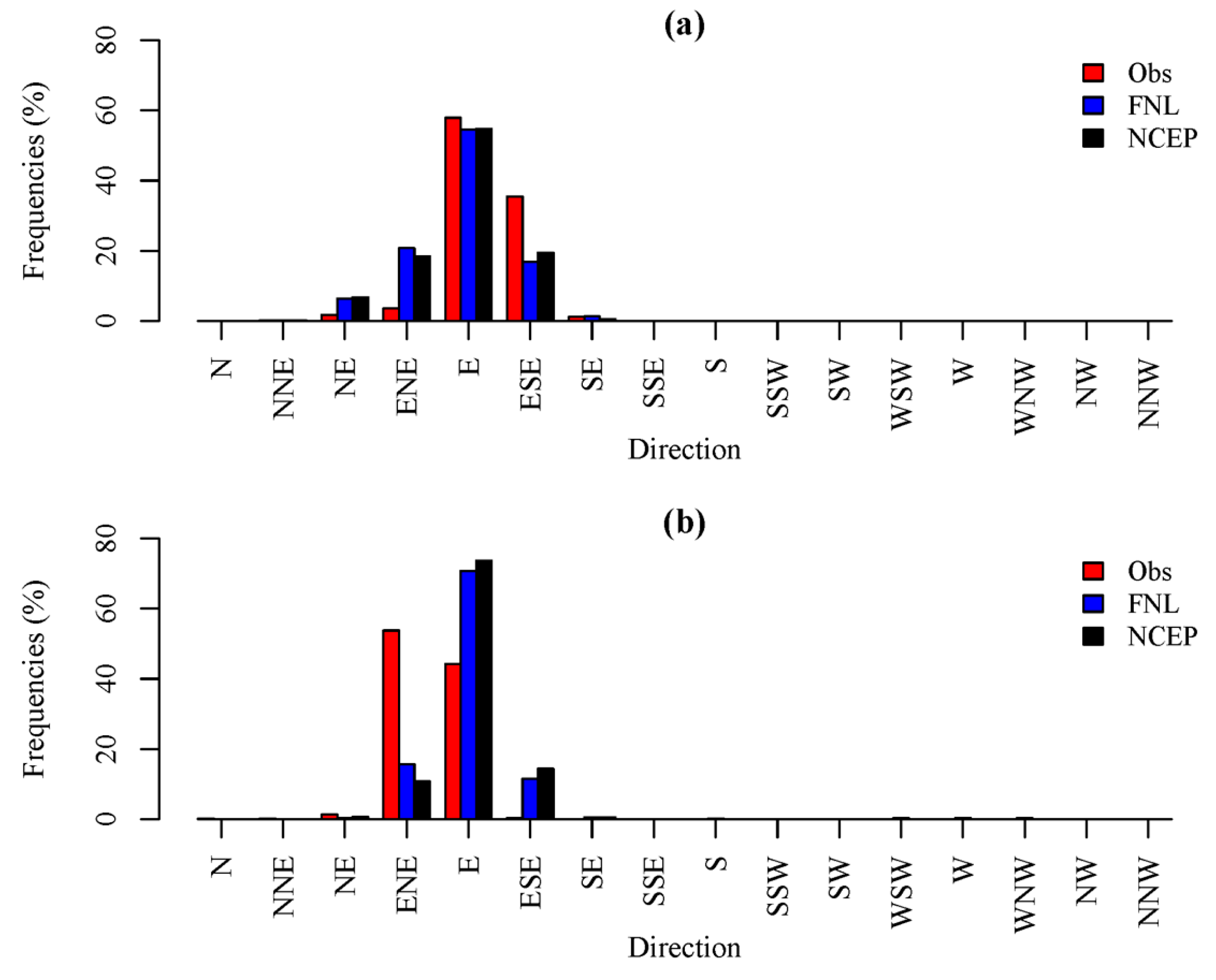
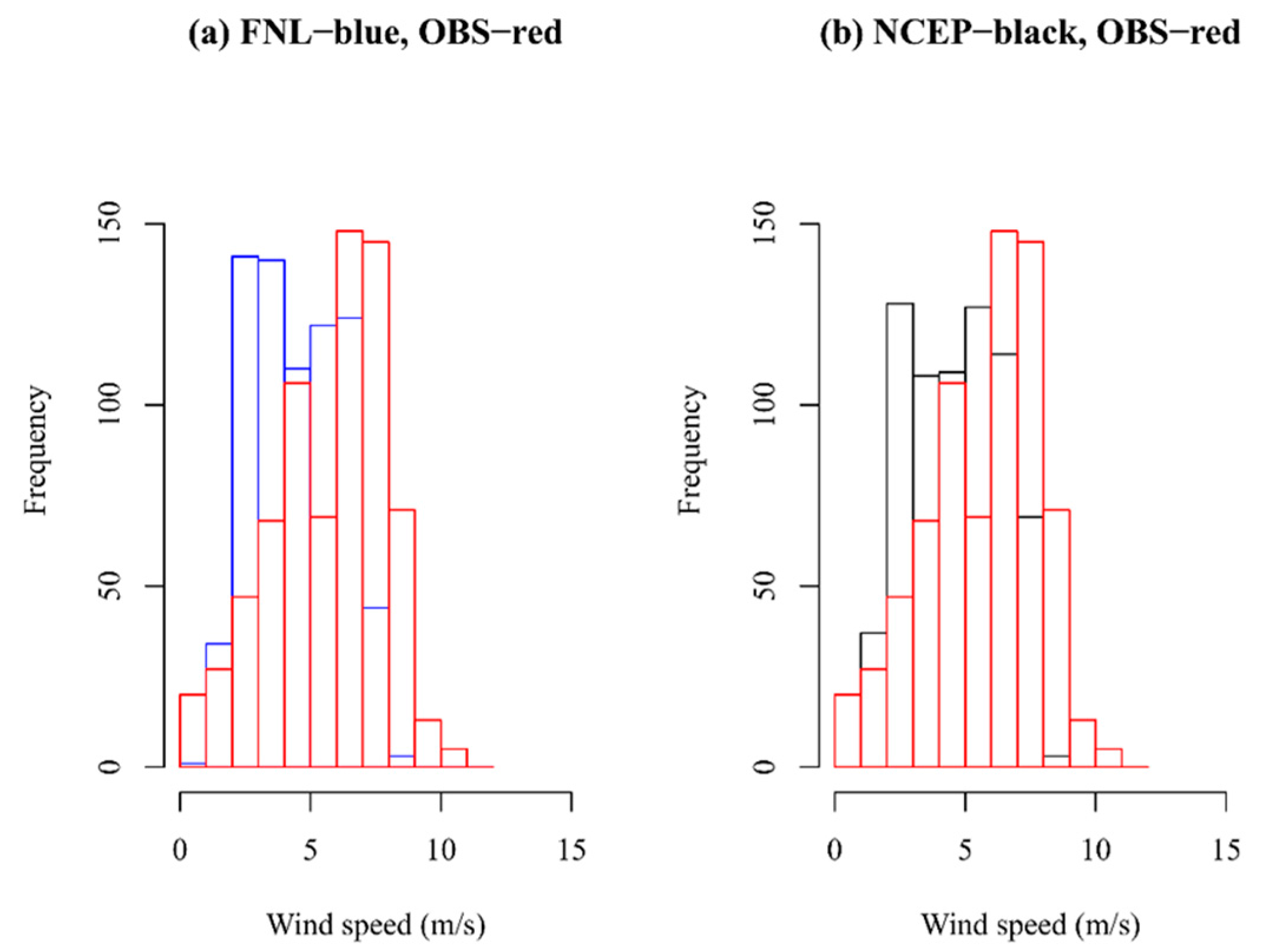
3.2.1. General Observations for Hourly Simulations of Wind Speed
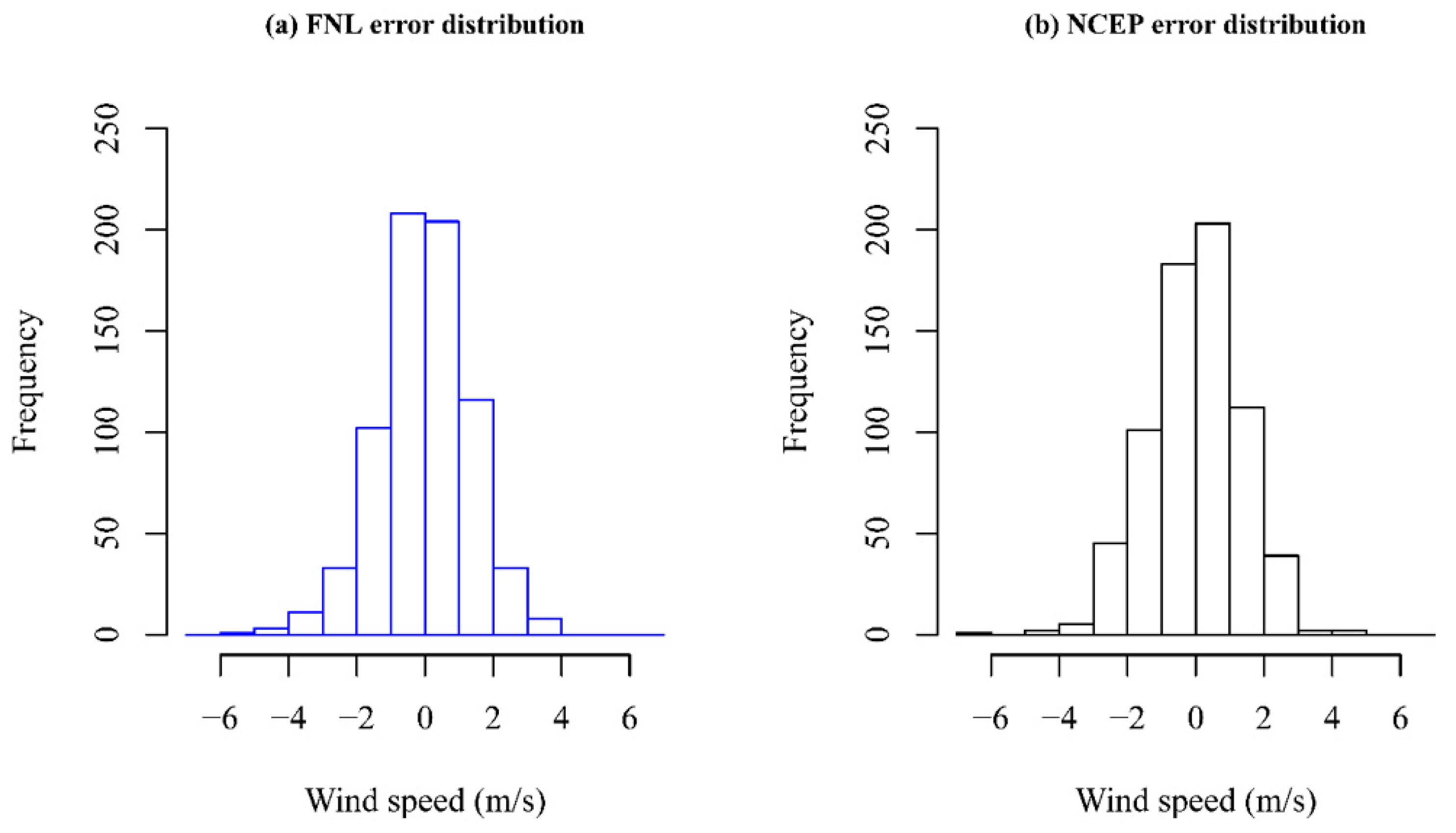
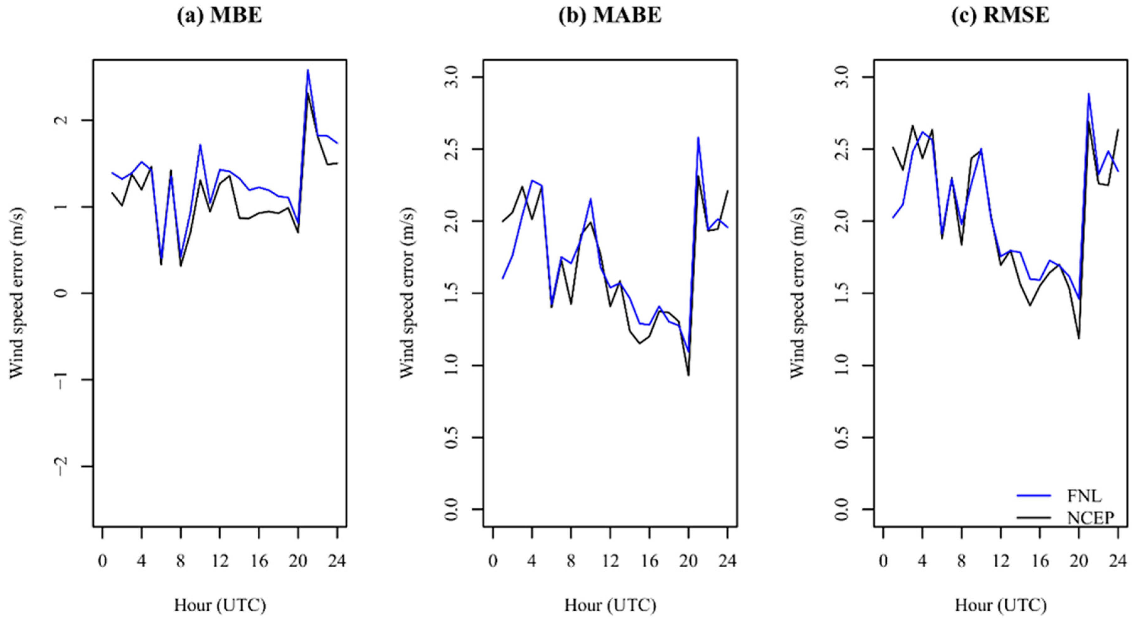
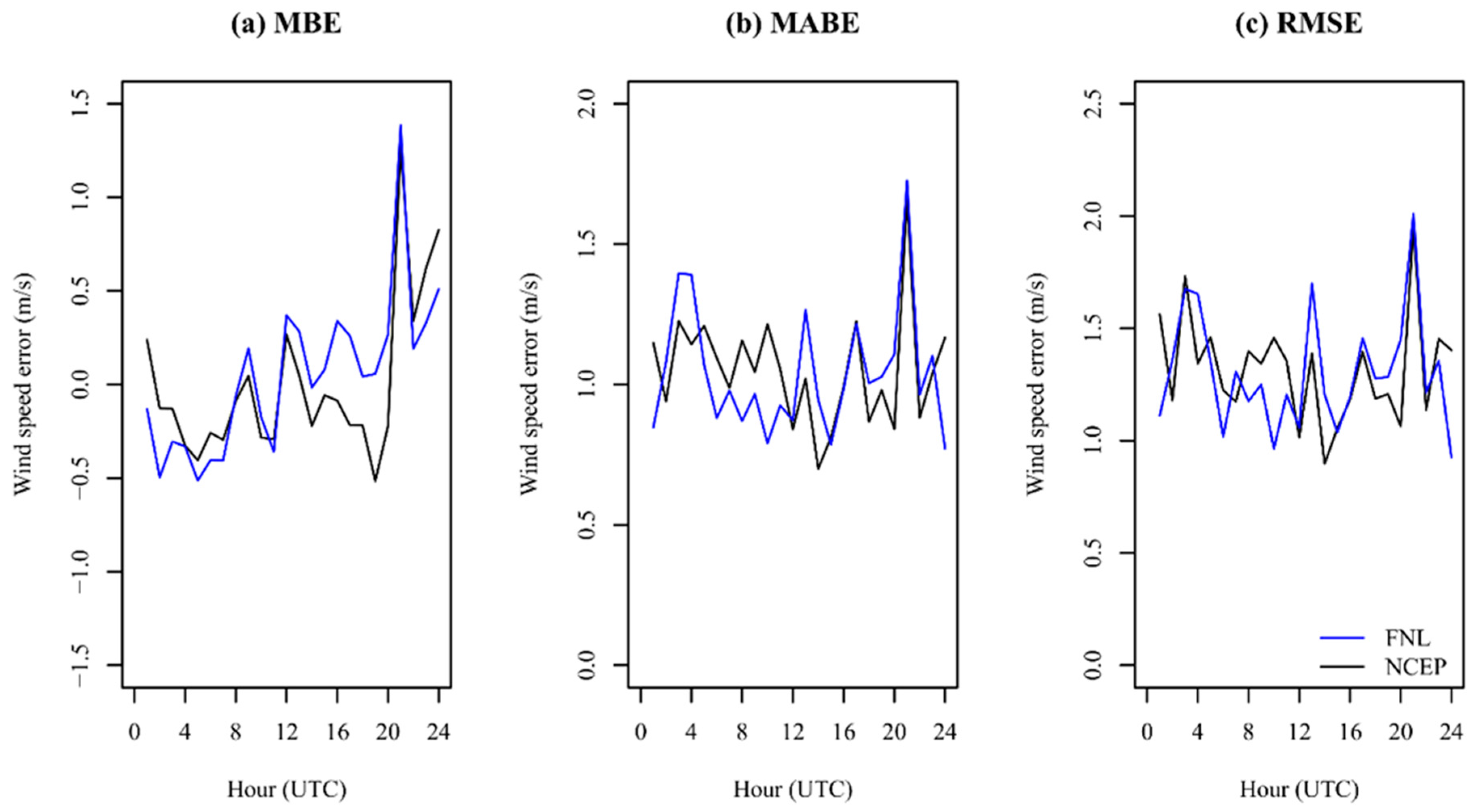
3.2.2. Error Statistics for FNL vs NCEP as Initial and Boundary Conditions
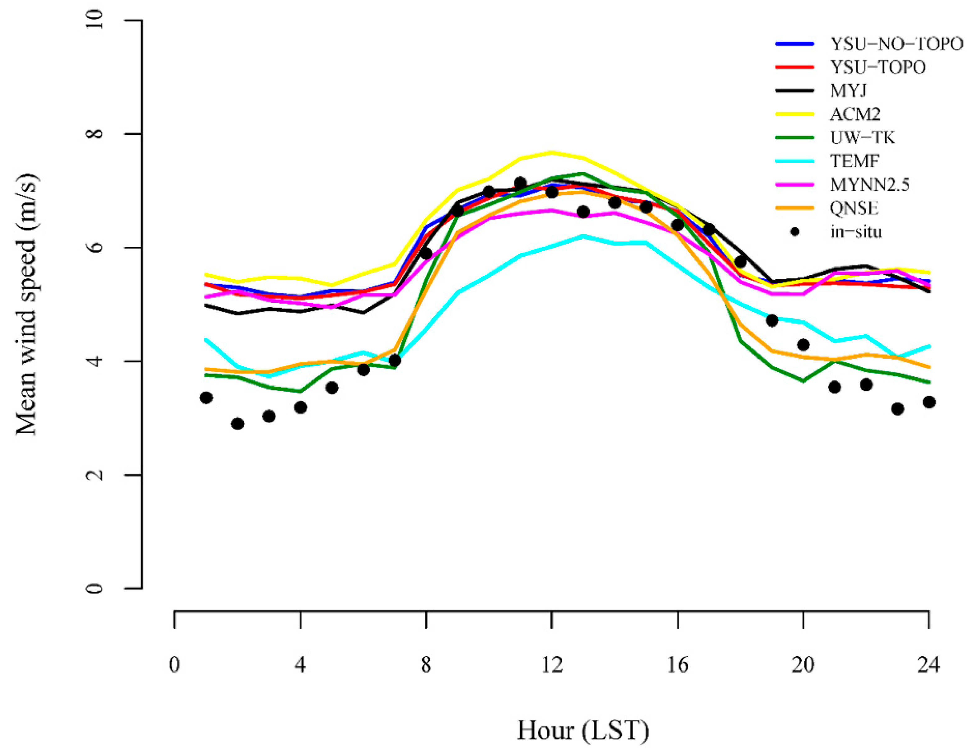
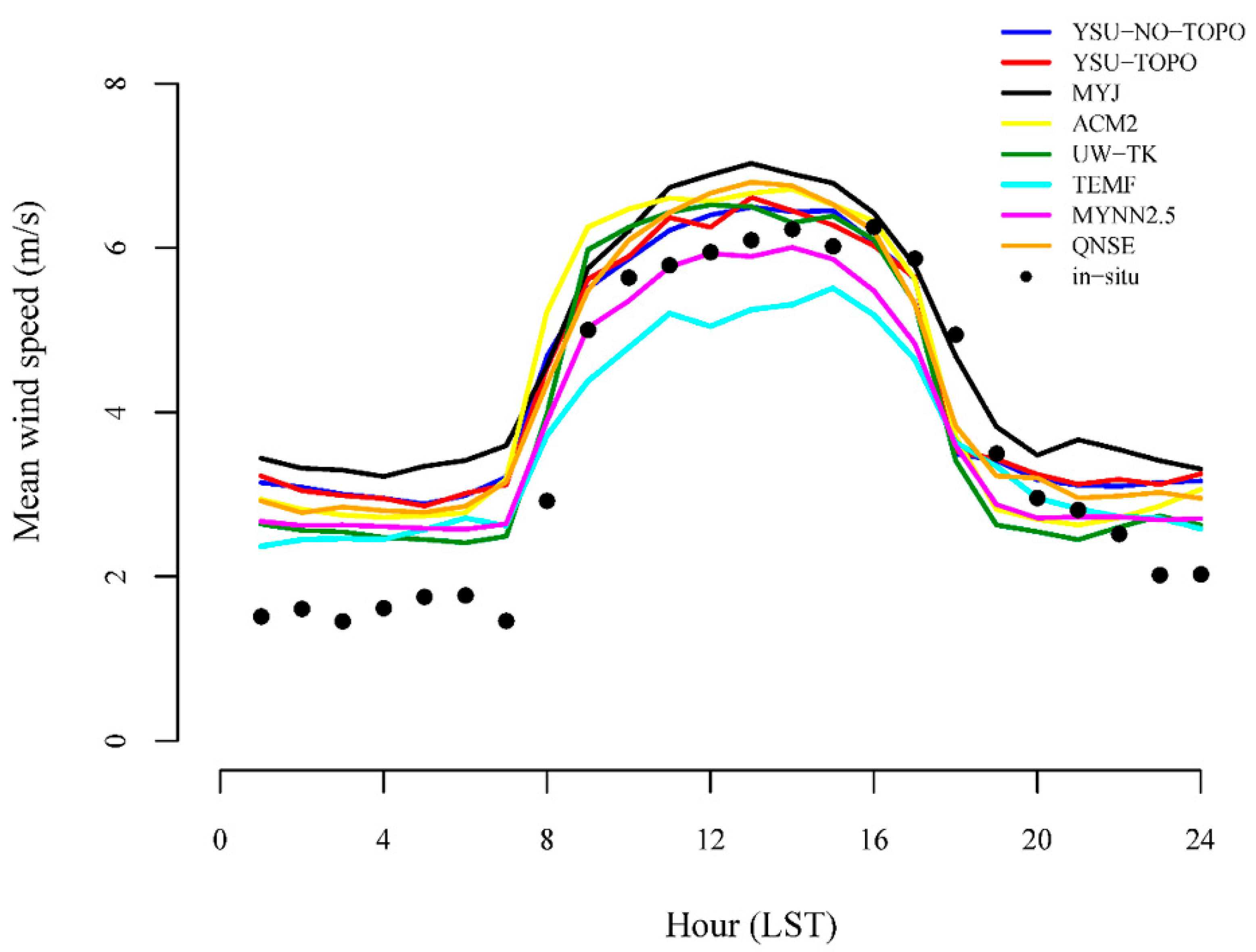
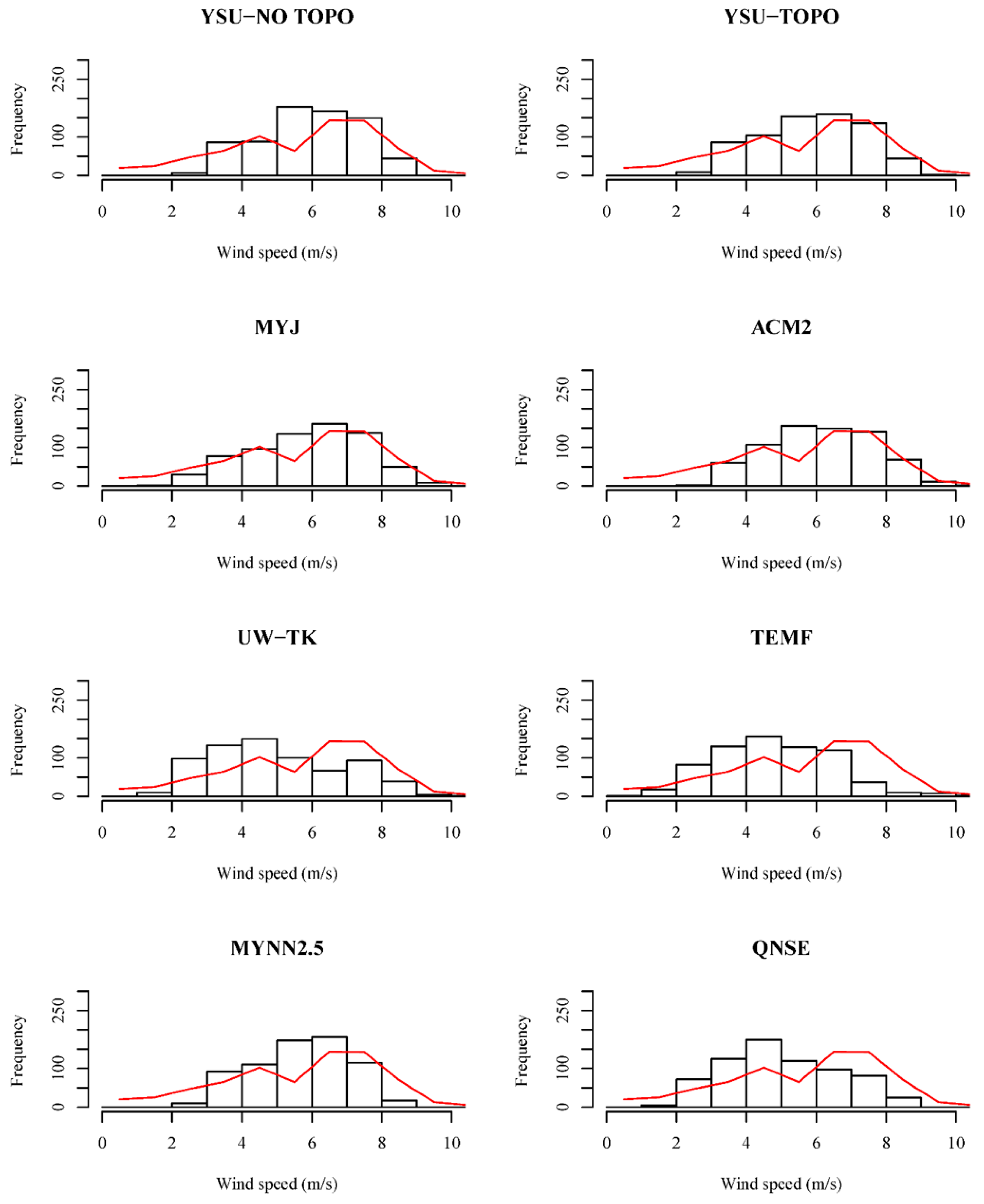
3.3. Sensitivity to PBL Schemes
4. Conclusions
Acknowledgments
Author Contributions
Conflicts of Interest
Appendix A. Description of Error Metrics
References
- Central Intelligence Agency (CIA). The World Factbook: Central America and Caribbean: Trinidad and Tobago. Available online: https://www.cia.gov/library/publications/the-world-factbook/geos/td.html (accessed on 12 May 2017).
- Barton, C.; Kendrick, L.; Humpert, M. The Caribbean Has Some of the World’s Highest Energy Costs—Now Is the Time to Transform the Region’s Energy Market. Available online: http://blogs.iadb.org/caribbean-dev-trends/2013/11/14/the-caribbean-has-some-of-theworlds-highest-energy-costs-now-is-the-time-to-transform-the-regions-energy-market/ (accessed on 16 November 2015).
- Ministry of Energy and Energy Affairs (GORTT). Framework for Development of a Renewable Energy Policy for Trinidad and Tobago. Available online: http://www.energy.gov.tt/wp-content/uploads/2014/01/Framework-for-the-development-of-a-renewable-energy-policy-for-TT-January-2011.pdf (accessed on 19 August 2013).
- IRENA. Renewable Power Generation Costs in 2014. Available online: https://www.irena.org/DocumentDownloads/Publications/IRENA_RE_Power_Costs_2014_report.pdf (accessed on 12 May 2017).
- IRENA. Global Atlas for Renewable Energy. Available online: http://irena.masdar.ac.ae/ (accessed on 16 April 2017).
- Vaisala. How Was the 5 km Global Wind Dataset Created? Available online: http://www.3tier.com/en/support/wind-prospecting-tools/how-was-data-behind-your-prospecting-map-created/ (accessed on 16 April 2017).
- DTU Department of Wind Energy. Global Wind Atlas. Available online: http://globalwindatlas.com/ (accessed on 16 April 2017).
- Potter, C.W.; Lew, D.; McCaa, J.; Cheng, S.; Eichelberger, S.; Grimit, E. Creating the dataset for the Western wind and solar integration study (USA). Wind Eng. 2008, 32, 325–338. [Google Scholar] [CrossRef]
- Yim, S.H.L.; Fung, J.C.H.; Lau, A.K.H.; Kot, S.C. Developing a high resolution wind map for a complex terrain with a coupled MM5/CALMET system. J. Geophys. Res. 2007, 112, D05106. [Google Scholar] [CrossRef]
- Dvorak, M.J.; Archer, C.L.; Jacobson, M.Z. California offshore wind energy potential. Renew. Energy 2010, 35, 1244–1255. [Google Scholar] [CrossRef]
- Larsén, X.G.; Mann, J.; Berg, J.; Göttel, H.; Jacob, D. Wind climate from the regional climate model REMO. Wind Energy 2010, 13, 279–296. [Google Scholar] [CrossRef]
- Frank, H.P.; Rathmann, O.; Mortensen, N.G.; Landberg, L. The Numerical Wind Atlas—The KAMM/WasP Method. Available online: http://orbit.dtu.dk/files/7728898/ris_r_1252.pdf (accessed 8 May 2017).
- Charabi, Y.; Al-Yahyai, S.; Gastli, A. Evaluation of NWP performance for wind energy resource assessment in Oman. Renew. Sustain. Energy Rev. 2011, 15, 1545–1555. [Google Scholar] [CrossRef]
- Kotroni, V.; Lagouvardos, K.; Lykoudis, S. High-resolution model-based wind atlas for Greece. Renew. Sustain. Energy Rev. 2014, 30, 479–489. [Google Scholar] [CrossRef]
- Yu, W.; Benoit, R.; Girard, C.; Glazer, A.; Lemarquis, D.; Salmon, J.R.; Pinard, J.-P. Wind energy simulation toolkit (WEST): A wind mapping system for use by the wind-energy industry. Wind Eng. 2006, 30, 15–33. [Google Scholar] [CrossRef]
- Draxl, C.; Hahmann, A.N.; Peña, A.; Giebel, G. Evaluating winds and vertical wind shear from weather research and forecasting model forecasts using seven planetary boundary layer schemes. Wind Energy 2014, 17, 39–56. [Google Scholar] [CrossRef]
- Giannakopoulou, E.-M.; Nhili, R. WRF model methodology for offshore wind energy applications. Adv. Meteorol. 2014, 2014, 319819. [Google Scholar] [CrossRef]
- Penchah, M.M.; Malakooti, H.; Satkin, M. Evaluation of planetary boundary layer simulations for wind resource study in East of Iran. Renew. Energy 2017, 111, 1–10. [Google Scholar] [CrossRef]
- Wootten, A.; Bowden, J.H.; Boyles, R.; Terando, A. The sensitivity of WRF downscaled precipitation in Puerto Rico to cumulus parameterization and interior grid nudging. J. Appl. Meteor. Climatol. 2016, 55, 2263–2281. [Google Scholar] [CrossRef]
- Whitehall, K.; Chiao, S.; Mayers-Als, M. Numerical investigations of convective initiation in Barbados. Adv. Meteorol. 2013, 2013, 630263. [Google Scholar] [CrossRef]
- Rama Rao, Y.V.; Alves, L.; Seulall, B.; Mitchell, Z.; Samaroo, K.; Cummings, G. Evaluation of the weather and forecasting (WRF) model over Guyana. Nat. Hazards 2012, 61, 1243–1261. [Google Scholar] [CrossRef]
- Yang, Z.; Taraphdar, S.; Wang, T.; Leung, L.R.; Grear, M. Uncertainty and feasibility of dynamical downscaling for modeling tropical cyclones for storm surge simulations. Nat. Hazards 2016, 84, 1161–1184. [Google Scholar] [CrossRef]
- Khain, A.; Lynn, B.; Shpund, J. High resolution WRF simulations of Hurricane Irene: Sensitivity to aerosols and choice of microphysics schemes. Atmos. Res. 2016, 167, 129–145. [Google Scholar] [CrossRef]
- Seroka, G.; Miles, T.; Xu, Y.; Kohut, J.; Schofield, O.; Glenn, S. Hurricane Irene sensitivity to stratified coastal ocean cooling. Mon. Weather Rev. 2016, 144, 3507–3530. [Google Scholar] [CrossRef]
- Carvalho, D.; Rocha, A.; Gómez-Gesteira, M.; Silva Santos, C. WRF wind simulation and wind energy production estimates forces by different reanalyses: Comparison with observed data for Portugal. Appl. Energy 2014, 117, 116–126. [Google Scholar] [CrossRef]
- Skamarock, W.C. Evaluating mesoscale NWP models using kinetic energy spectra. Mon. Weather Rev. 2004, 132, 3019–3031. [Google Scholar] [CrossRef]
- Carvalho, D.; Rocha, A.; Gómez-Gesteira, M.; Santos, C. A sensitivity study of the WRF model in wind simulation for an area of high wind energy. Environ. Modell. Softw. 2012, 33, 23–34. [Google Scholar] [CrossRef]
- Wen, M.; Yang, S.; Vintzileos, A.; Higgins, W.; Zhang, R. Impacts of model resolutions and initial conditions on predictions of the Asian summer monsoon by the NCEP Climate Forecast System. Weather Forecast. 2012, 27, 629–646. [Google Scholar] [CrossRef]
- Environment Canada. Canadian Wind Energy Atlas at 5 km. Available online: http://www.windatlas.ca or http://collaboration.cmc.ec.gc.ca/science/rpn/modcom/eole/ (accessed on 10 August 2014).
- Kalnay, E.; Kanamitsu, M.; Kistler, R.; Collins, W.; Deaven, D.; Gandin, L.; Iredell, M.; Saha, S.; White, G.; Woollen, J.; et al. The NCEP/NCAR 40-year reanalysis project. Bull. Am. Meteor. Soc. 1996, 77, 437–470. [Google Scholar] [CrossRef]
- Nunalee, C.G.; Basu, S. Mesoscale modeling of coastal low-level jets: Implications for offshore wind resource estimation. Wind Energy 2013, 17, 1199–1216. [Google Scholar] [CrossRef]
- Berrisford, P.; Dee, D.; Poli, P.; Brugge, R.; Fielding, K.; Fuentes, M.; Kållberg, P.; Kobayashi, S.; Uppala, S.; Simmons, A. The ERA-Interim Archive. Available online: https://www.ecmwf.int/en/library/8174-era-interim-archive-version-20 (accessed on 6 June 2017).
- Chadee, X.T.; Clarke, R.M. Large-scale wind energy potential of the Caribbean region using near-surface reanalysis data. Renew. Sustain. Energy Rev. 2014, 30, 45–58. [Google Scholar] [CrossRef]
- Kanamitsu, M.; Ebisuzaki, W.; Woollen, J.; Yang, S.-K.; Hnilo, J.J.; Fiorino, M.; Potter, G.L. NCEP-DOE AMIP-II Reanalysis (R-2). Bull. Am. Meteor. Soc. 2002, 83, 1631–1643. [Google Scholar] [CrossRef]
- NCEP FNL Operational Model Global Tropospheric Analyses, Continuing from July 1999. Available online: https://doi.org/10.5065/D6M043C6 (accessed on 6 June 2017).
- NCEP. GFS/GDAS Changes Since 1991. Available online: http://www.emc.ncep.noaa.gov/gmb/STATS/html/model_changes.html (accessed on 17 April 2017).
- Petersen, E.L.; Troen, I. Wind conditions and resource assessment. WIREs Energy Environ. 2012, 1, 206–217. [Google Scholar] [CrossRef]
- Larsén, X.G.; Badger, J.; Hahmann, A.N.; Mortensen, N.G. The selective dynamical downscaling method for extreme-wind atlases. Wind Energy 2013, 16, 1167–1182. [Google Scholar] [CrossRef]
- Zack, J.; Natenberg, E.J.; Knowe, G.V.; Manobianco, J.; Waight, K.; Hanley, D.; Kamath, C. Use of Data Denial Experiments to Evaluate ESA Forecast Sensitivity Patterns. Available online: http://ckamath.org/yahoo_site_admin/assets/docs/LLNL-TR-499166.298232948.pdf (accessed on 19 June 2017).
- Al-Yahyai, S.; Charabi, Y.; Al-Badi, A.; Gastli, A. Nested ensemble NWP approach for wind energy assessment. Renew. Energy 2012, 37, 150–160. [Google Scholar] [CrossRef]
- Beaucage, P.; Brower, M.C.; Tensen, J. Evaluation of four numerical wind flow models for wind resource mapping. Wind Energy 2014, 17, 197–208. [Google Scholar] [CrossRef]
- Huva, R.; Dargaville, R.; Caine, S. Prototype large-scale renewable energy system optimisation for Victoria, Australia. Energy 2012, 41, 326–334. [Google Scholar] [CrossRef]
- Santos-Alamillos, F.J.; Pozo-Vázquez, D.; Ruiz-Arias, J.A.; Lara-Farego, V.; Tovar-Pescador, J. Analysis of WRF model wind estimate sensitivity to physics parameterization choice and terrain representation in Andalusia (Southern Spain). J. Appl. Meteorol. Climatol. 2013, 52, 1592–1609. [Google Scholar] [CrossRef]
- Marrero, C.; Jorba, O.; Cuevas, E.; Baldasano, J.M. Sensitivity study of surface wind flow of a limited area model simulating the extratropical storm Delta affecting the Canary Islands. Adv. Sci. Res. 2008, 2, 151–157. [Google Scholar] [CrossRef]
- Mohan, M.; Bhati, S. Analysis of WRF model performance over subtropical region of Delhi, India. Adv. Meteorol. 2011, 2011, 621235. [Google Scholar] [CrossRef]
- Storm, B.; Basu, S. The WRF model forecast-derived low-level wind shear climatology over the United States Great Plains. Energies 2010, 3, 258–276. [Google Scholar] [CrossRef]
- Woods, B.; Nehrkorn, T.; Henderson, J. A downscaled wind climatology on the Outer Continental Shelf. J. Appl. Meteorol. Climatol. 2013, 52, 1878–1890. [Google Scholar] [CrossRef]
- Amjad, M.; Zafar, Q.; Khan, F.; Sheikh, M.M. Evaluation of weather research and forecasting model for the assessment of wind resource over Gharo, Pakistan. Int. J. Climatol. 2015, 35, 1821–1832. [Google Scholar] [CrossRef]
- Nawri, N.; Petersen, G.N.; Bjornsson, H.; Hahmann, A.N.; Jónasson, K.; Hasager, C.; Clausen, N.-E. The wind energy potential of Iceland. Renew. Energy 2014, 69, 290–299. [Google Scholar] [CrossRef]
- National Climatic Data Center. Data Access. Available online: https://www.ncdc.noaa.gov/data-access (accessed on 29 November 2012).
- Jiménez-Guerrero, P.; Jorba, O.; Baldasano, J.M.; Gassó, S. The use of a modelling system as a tool for air quality management: Annual high-resolution simulations and evaluation. Sci. Total Environ. 2008, 390, 323–340. [Google Scholar] [CrossRef] [PubMed]
- Legates, D.R.; McCabe, G.J., Jr. Evaluating the use of “goodness-of-fit” measures in hydrologic and hydroclimatic model validation. Water Resour. Res. 1999, 35, 233–241. [Google Scholar] [CrossRef]
- Chu, Y.; Li, C.; Wang, Y.; Li, J.; Li, J. A long-term wind speed ensemble forecasting system with weather adapted correction. Energies 2016, 9, 894. [Google Scholar] [CrossRef]
- Skamarock, W.C.; Klemp, J.B.; Dudhia, J.; Gill, D.O.; Barker, D.M.; Duda, M.G.; Huang, X.-Y.; Wang, W.; Powers, J.G. A Description of the Advanced Research WRF Version 3. Available online: http://www2.mmm.ucar.edu/wrf/users/docs/arw_v3.pdf (accessed on 12 October 2013).
- Hong, S.-Y.; Noh, Y.; Dudhia, J. A new vertical diffusion package with an explicit treatment of entrainment processes. Mon. Weather Rev. 2006, 134, 2318–2341. [Google Scholar] [CrossRef]
- Pleim, J.E. A combined local and non-local closure model for the atmospheric boundary layer. Part I: Model description and testing. J. Appl. Meteorol. Climatol. 2007, 46, 1383–1395. [Google Scholar] [CrossRef]
- Janjic, Z.I. The Step-Mountain Eta Coordinate model: Further developments of the convection, viscous sublayer, and turbulence closure schemes. Mon. Weather Rev. 1994, 122, 927–945. [Google Scholar] [CrossRef]
- Nakanishi, M.; Niino, H. An improved Mellor-Yamada level 3 model: Its numerical stability and application to a regional prediction of advecting fog. Bound. Layer Meteorol. 2006, 119, 397–407. [Google Scholar] [CrossRef]
- Nakanishi, M.; Niino, H. Development of an improved turbulence closure model for the atmospheric boundary layer. J. Meteorol. Soc. Jpn. 2009, 87, 895–912. [Google Scholar] [CrossRef]
- Sukoriansky, S.; Galperin, B.; Perov, V. Application of a new spectral model of stratified turbulence to the atmospheric boundary layer over sea ice. Bound. Layer Meteorol. 2005, 119, 397–407. [Google Scholar]
- Bretherton, C.S.; Park, S. A new moist turbulence parameterization in the Community Atmosphere Model. J. Clim. 2009, 22, 3422–3448. [Google Scholar] [CrossRef]
- Angevine, W.M.; Jiang, H.; Mauritsen, T. Performance of an eddy diffusivity-mass flux scheme for shallow cumulus boundary layers. Mon. Weather Rev. 2010, 138, 2895–2912. [Google Scholar] [CrossRef]
- Nastrom, G.D.; Gage, K.S. A climatology of atmospheric wavenumber spectra of wind and temperature observed by commercial aircraft. J. Atmos. Sci. 1985, 58, 3424–3442. [Google Scholar] [CrossRef]
- Cho, J.Y.N.; Zhu, Y.; Newell, R.E.; Anderson, B.E.; Barrick, J.D.; Gregory, G.L.; Sachse, G.W.; Carroll, M.A.; Albercook, G.M. Horizontal wavenumber spectra of winds, temperature, and trace gases during the Pacific Exploratory Missions: 1. Climatology. J. Geophys. Res. Atmos. 1999, 104, 5697–5716. [Google Scholar] [CrossRef]
- Cho, J.Y.N.; Newell, R.E.; Barrick, J.D. Horizontal wavenumber spectra of winds, temperature, and trace gases during the Pacific Exploratory Missions: 2. Gravity waves, quasi-two-dimensional turbulence, and vortical models. J. Geophys. Res. Atmos. 1999, 104, 16297–16308. [Google Scholar] [CrossRef]


| Statistic | Piarco | Crown Point | ||
|---|---|---|---|---|
| FNL | NCEP | FNL | NCEP | |
| Mean predicted wind speed (m/s) | 4.06 | 4.10 | 4.45 | 4.64 |
| Mean observed wind speed (m/s) | 4.10 | 4.10 | 5.77 | 5.77 |
| Mean bias error (MBE) (m/s) | 0.05 | −0.01 | 1.32 | 1.13 |
| Mean absolute error (MABE) (m/s) | 1.04 | 1.05 | 1.72 | 1.70 |
| RMSE (m/s) | 1.33 | 1.34 | 2.11 | 2.11 |
| R2 | 0.61 | 0.62 | 0.45 | 0.38 |
| IOA | 0.88 | 0.89 | 0.73 | 0.73 |
| 17° | 16° | 13° | 15° | |
| 27° | 20° | 17° | 19° | |
| 13° | 15° | −9° | −9° | |
| Statistic | Piarco | |||||||
|---|---|---|---|---|---|---|---|---|
| YSU-NO-TOPO | YSU-TOPO | MYJ | ACM2 | UW-TK | TEMF | MYNN 2.5 | QNSE | |
| Mean observed wind speed (m/s) | 4.10 | 4.10 | 4.10 | 4.10 | 4.10 | 4.10 | 4.10 | 4.10 |
| Mean predicted wind speed (m/s) | 4.32 | 4.32 | 4.69 | 4.31 | 4.01 | 3.64 | 3.85 | 4.29 |
| Mean bias error (MBE) (m/s) | +0.22 | +0.22 | +0.59 | +0.19 | −0.08 | −0.45 | −0.25 | +0.19 |
| RMSE (m/s) | 1.33 | 1.32 | 1.47 | 1.30 | 1.28 | 1.62 | 1.28 | 1.34 |
| Mean absolute error (MABE) (m/s) | 1.04 | 1.03 | 1.16 | 1.03 | 1.03 | 1.27 | 1.02 | 1.05 |
| STDE | 1.31 | 1.30 | 1.34 | 1.28 | 1.28 | 1.56 | 1.26 | 1.33 |
| R2 | 0.61 | 0.61 | 0.58 | 0.62 | 0.62 | 0.44 | 0.64 | 0.59 |
| IOA | 0.87 | 0.87 | 0.84 | 0.88 | 0.89 | 0.78 | 0.87 | 0.87 |
| Observed wind power density (WPD) (W m−2) | 74.9 | 74.9 | 74.9 | 74.9 | 74.9 | 74.9 | 74.9 | 74.9 |
| Predicted WPD (W m−2) | 72.1 | 72.4 | 88.9 | 78.9 | 68.3 | 46.2 | 52.8 | 75.5 |
| Statistic | Crown Point | |||||||
|---|---|---|---|---|---|---|---|---|
| YSU-NO-TOPO | YSU-TOPO | MYJ | ACM2 | UW-TK | TEMF | MYNN 2.5 | QNSE | |
| Mean observed wind speed (m/s) | 5.77 | 5.77 | 5.76 | 5.77 | 5.76 | 5.77 | 5.77 | 5.76 |
| Mean predicted wind speed (m/s) | 5.92 | 5.88 | 5.90 | 6.16 | 5.00 | 4.83 | 5.71 | 5.03 |
| Mean bias error (MBE) (m/s) | +0.16 | +0.12 | +0.15 | +0.39 | −0.76 | −0.92 | −0.06 | −0.74 |
| RMSE (m/s) | 1.75 | 1.73 | 1.78 | 1.76 | 1.92 | 2.25 | 1.81 | 1.83 |
| Mean absolute error (MABE) (m/s) | 1.37 | 1.39 | 1.42 | 1.40 | 1.52 | 1.81 | 1.47 | 1.48 |
| STDE | 1.74 | 1.73 | 1.77 | 1.72 | 1.76 | 2.05 | 1.81 | 1.67 |
| R2 | 0.37 | 0.38 | 0.37 | 0.40 | 0.40 | 0.22 | 0.34 | 0.42 |
| IOA | 0.74 | 0.75 | 0.76 | 0.75 | 0.77 | 0.66 | 0.71 | 0.76 |
| Observed wind power density (WPD) (W m−2) | 165.6 | 165.6 | 165.6 | 165.6 | 165.6 | 165.6 | 165.6 | 165.6 |
| Predicted WPD (W m−2) | 149.4 | 147.6 | 153.8 | 168.5 | 109.7 | 96.2 | 132.7 | 102.2 |
| Statistic | Average Spatial Error for Each PBL Scheme | |||||||
|---|---|---|---|---|---|---|---|---|
| YSU-NO-TOPO | YSU-TOPO | MYJ | ACM2 | UW-TK | TEMF | MYNN 2.5 | QNSE | |
| Mean bias error (MBE) (m/s) | +0.19 | +0.16 | +0.37 | +0.29 | −0.42 | −0.69 | −0.16 | −0.28 |
| RMSE (m/s) | 1.54 | 1.53 | 1.63 | 1.53 | 1.60 | 1.94 | 1.55 | 1.59 |
| Mean absolute error (MABE) (m/s) | 1.21 | 1.21 | 1.29 | 1.22 | 1.28 | 1.54 | 1.25 | 1.27 |
| STDE | 1.53 | 1.52 | 1.56 | 1.50 | 1.52 | 1.81 | 1.55 | 1.50 |
© 2017 by the authors. Licensee MDPI, Basel, Switzerland. This article is an open access article distributed under the terms and conditions of the Creative Commons Attribution (CC BY) license (http://creativecommons.org/licenses/by/4.0/).
Share and Cite
Chadee, X.T.; Seegobin, N.R.; Clarke, R.M. Optimizing the Weather Research and Forecasting (WRF) Model for Mapping the Near-Surface Wind Resources over the Southernmost Caribbean Islands of Trinidad and Tobago. Energies 2017, 10, 931. https://doi.org/10.3390/en10070931
Chadee XT, Seegobin NR, Clarke RM. Optimizing the Weather Research and Forecasting (WRF) Model for Mapping the Near-Surface Wind Resources over the Southernmost Caribbean Islands of Trinidad and Tobago. Energies. 2017; 10(7):931. https://doi.org/10.3390/en10070931
Chicago/Turabian StyleChadee, Xsitaaz T., Naresh R. Seegobin, and Ricardo M. Clarke. 2017. "Optimizing the Weather Research and Forecasting (WRF) Model for Mapping the Near-Surface Wind Resources over the Southernmost Caribbean Islands of Trinidad and Tobago" Energies 10, no. 7: 931. https://doi.org/10.3390/en10070931