
Minimization of Construction Costs for an All Battery-Swapping Electric-Bus Transportation System: Comparison with an All Plug-In System

1
Department of Tourism and Leisure, National Penghu University of Science and Technology, Makung 880, Taiwan
2
Department of Electrical Engineering, National Penghu University of Science and Technology, Makunk 880, Taiwan
*
Author to whom correspondence should be addressed.
Energies 2017, 10(7), 890; https://doi.org/10.3390/en10070890
Submission received: 12 April 2017
/
Revised: 23 June 2017
/
Accepted: 26 June 2017
/
Published: 30 June 2017
Abstract
:The greenhouse gases and air pollution generated by extensive energy use have exacerbated climate change. Electric-bus (e-bus) transportation systems help reduce pollution and carbon emissions. This study analyzed the minimization of construction costs for an all battery-swapping public e-bus transportation system. A simulation was conducted according to existing timetables and routes. Daytime charging was incorporated during the hours of operation; the two parameters of the daytime charging scheme were the residual battery capacity and battery-charging energy during various intervals of daytime peak electricity hours. The parameters were optimized using three algorithms: particle swarm optimization (PSO), a genetic algorithm (GA), and a PSO–GA. This study observed the effects of optimization on cost changes (e.g., number of e-buses, on-board battery capacity, number of extra batteries, charging facilities, and energy consumption) and compared the plug-in and battery-swapping e-bus systems. The results revealed that daytime charging can reduce the construction costs of both systems. In contrast to the other two algorithms, the PSO–GA yielded the most favorable optimization results for the charging scheme. Finally, according to the cases investigated and the parameters of this study, the construction cost of the plug-in e-bus system was shown to be lower than that of the battery-swapping e-bus system.
1. Introduction
Global warming and climate change have led to extreme changes in weather conditions in recent years. In addition, the rapid growth of human activities has accelerated the depletion of traditional petrochemical energy sources, resulting in severe ecological, environmental, and economic threats and impacts. Therefore, carbon reduction has become a formidable challenge in the 21st century. Numerous countries have actively implemented countermeasures against local greenhouse gas emissions [1,2,3]. Green policies should be actively promoted to create sustainable employment opportunities, implement environmental sustainability, and establish a low-carbon society with a low-carbon economy as the goal.
The Penghu Islands (23°33′ N, 119°35′ E) are located in the Taiwan Strait, approximately 44 km west of Taiwan. The total area of the archipelago is approximately 128 km2, and it has a population of approximately 100,000. The Penghu Low Carbon Island Project began in 2011 with the aim to transform the archipelago through eight dimensions, namely renewable energy, energy conservation, green transportation, low-carbon construction, resource recycling, environmental greening, low-carbon living, and low-carbon education [4]. The impetus of this study was the promotion of electric buses (e-buses) in the green transportation section of the Penghu Low Carbon Island Project. The use of public transportation vehicles in the confined Penghu Islands will substantially increase as the tourism industry develops. The exhaust gas emitted by conventional diesel-powered vehicles is a source of air pollution, and reducing the emissions of these diesel-powered vehicles will improve the air quality. Public transport operators in Taiwan have begun promoting low-carbon transportation with hybrid e-buses. Although these hybrid e-buses consume fewer resources and generate less carbon emissions than diesel-powered buses do, they still emit carbon dioxide. A pure electric bus can run without generating any carbon dioxide and creates no environmental burden throughout the service route. Replacing all diesel buses in the Penghu Islands with e-buses could thus alleviate vehicle-generated carbon emissions [5,6,7]. Coupled with other green transportation equipment, a green traffic network can conserve energy by reducing carbon emissions, alleviate environmental hazards caused by human activities, and establish a comfortable living environment.
1.1. Literature Review
In response to breakthroughs in battery technology, automotive manufacturers have been investing in low-carbon electric vehicle development [8,9,10,11]. Electric vehicle manufacturing technology has matured in Taiwan because of the competitive electrical and electronics industry and the complete integration of the industrial chain. The two types of e-bus charging equipment are plug-in e-buses (PI-Ebus) and battery-swapping e-buses (BS-Ebus). Charging specifications differ according to the e-bus type. In addition, charging schemes generally comprise slow-charging and fast-charging models. The slow-charging model provides the battery with the current appropriate for its characteristics. This can prolong battery life, enable charging during off-peak hours, and lower the charging costs. However, the long charging hours may prevent it from meeting the operating demand [12,13,14,15]. The fast-charging model can provide 80–90% battery capacity in a short time by supplying a substantial amount of current. However, this involves a higher level of charging technology, greater safety requirements, and higher charging costs than the slow-charging model does [16,17,18].
Used batteries from BS-Ebuses can be quickly swapped with fully-charged ones. In addition, battery life assessment and fault detection can be conducted in battery-swapping facilities to prevent battery shortage [19]. However, the construction costs for battery-swapping facilities are high, and users must understand how to operate the battery-swapping model to ensure the normal operation of the system.
Genetic algorithms (GA) solve optimization problems through the process of natural selection [20,21]. The advantages of a GA include the abilities to: (1) encode decision variables as operators; (2) directly search the objective function; (3) search multiple signals simultaneously; and (4) utilize the probability search technique [22]. In this study, a GA was used to cooperate with the hybrid powertrain and calculate the optimal power management offline [23,24].
Particle swarm optimization (PSO), developed by Kennedy and Eberhart [25,26], is an algorithm based on swarm intelligence. PSO features advantages such as fast convergence, relatively few parameters, and suitability for dynamic environments [27]. Population-based PSO has attracted increasing attention because it is highly efficient and can search for global optimal solutions in scientific and engineering domains [27,28].
Compared with GAs, which no longer consider previous knowledge after each evolution, PSO can remember satisfactory solutions by using all its particles [29]. Moreover, the evolution of a GA is based on reproduction, crossover, and mutation. Therefore, a high computation load is required. By contrast, because the unique information diffusion and interaction mechanisms of PSO are comparably simple, a low computational burden is required, and the PSO is suitable for use in various applications such as control, system identification, network optimization, and electric power systems. Because the optimal and mean fitness of PSO populations do not easily converge to the same value, new GA-generated particles are employed in later iterations to expand the search range and obtain the global optimum through PSO–GA [30,31].
1.2. Motivation and Contributions
This study investigated the cost of e-bus construction to the public bus transportation system in the Penghu Islands. In contrast to conventional vehicles, e-buses feature the advantages of fuel efficiency, environmental friendliness, and low noise pollution; moreover, they benefit from electrical efficiency enhanced by power grid storage systems consisting of battery modules. The BS-Ebus system operation was simulated using a daytime charging option during e-bus operating hours. Through an optimized charging scheme, this study analyzed the effects of the number of buses in operation, battery capacity, the number of additional batteries, and the cost fluctuation of charging facilities and power consumption. Subsequently, the minimized construction cost was obtained through optimization using three algorithms: PSO, a GA, and a PSO–GA. Finally, this study compared the results of the BS-Ebus and PI-Ebus systems.
2. System Modeling and the Calculation of Construction Costs for a Battery-Swapping Electric-Buses Transportation System
The authors of this study previously proposed a PI-Ebus model for construction cost calculation [32]. This study adapted the aforementioned system modeling techniques to meet the requirements of a BS-Ebus model. The on-board batteries of PI-Ebuses cannot be detached and are recharged at charging stations [33]. These charging stations can be installed in e-bus parking lots without the need to construct additional facilities, thereby reducing the land cost. However, charging e-buses cannot be dispatched until the completion of the charging process, thereby decreasing the vehicle utilization rate. Consequently, additional costs are incurred to purchase a sufficient number of e-buses for bus operation throughout the day. In the BS-Ebus system, e-buses quickly complete battery switches through a battery-swapping system. In contrast to the PI-Ebus system, the e-buses in the BS-Ebus system can be immediately dispatched after the battery switch, thereby increasing the utilization rate. However, battery-swapping facilities and additional back-up batteries are required in the BS-Ebus system, thereby increasing the equipment costs.
This study tested the slow-charging model during nighttime off-peak hours (i.e., 22:30–07:30) because of the high electricity price during peak hours. All e-buses were fully charged in the morning before the bus service commenced. Although the daytime charging hours were designated as between 06:00 and 18:00, actual daytime charging began after 08:00. The daytime charging scheme in this study varied by e-bus type, including hourly or quarter-hour residual battery capacity (RBC) and battery-charging energy (BCE). The undispatched e-buses in the depot were inspected in intervals of 15 min or 1 h to determine whether the RBC was lower than the assigned value. A fast charge was conducted to increase the BCE according to the assigned value if the RBC was lower than the assigned value.
2.1. Modeling a Battery-Swapping Electric-Buses Transportation System
In the BS-Ebus system, the e-bus operating model was formulated according to the existing bus schedule. The e-bus operating and charging schedules were established according to four sequences, namely operation–line, bus number–line, e-bus battery capacity, and e-bus charging. The similarities and differences between the BS-Ebus and PI-Ebus systems in this study are described as follows:
- (1)
- The operating models in both systems were formulated according to the existing bus schedule. However, because the two models required different durations for recharging and battery swapping, the operation–line and number–line sequence diagrams varied between the two systems.
- (2)
- Both systems required fast charging during daytime and slow charging during nighttime. Because they required different charging equipment and back-up batteries, the battery capacity and recharging sequence diagrams varied between the two systems.
- (3)
- The round-trip durations in both systems were 20 min (10 min for each one-way trip), and each bus required 10 min for changing destination signs, cleaning, and driver change before being redispatched. The PI-Ebuses were recharged immediately at the charging station in the depot upon their return, whereas the BS-Ebuses required 15 min for battery swap according to the e-bus manufacturers.
- (4)
- Identical fast- and slow-charging curves were employed in both systems. To prolong the battery life, the minimum battery capacity of the on-board batteries was maintained at ≥20% in both systems.
- (5)
- The optimization parameters of the PI-Ebus system were RBC and battery-charging time (BCT), whereas those of the BS-Ebus system were RBC and BCE.
- (6)
- The electricity costs of the two e-bus systems were calculated according to the latest price quoted by Taipower Company.
- (7)
- The research considers a complex problem spanning the life expectancy of batteries. Some assumptions have been made, including no disruptions, schedule-based operations, and installation of a unique charging point. The costs are based on expected values, and no reliability analysis was fulfilled.
- (8)
- Because of the complexity of road and traffic conditions, a microscopic simulation could not be executed in this study. The energy consumption of each e-bus line was calculated by the constant energy consumption rate per kilometer. The energy consumption rates per kilometer were 1.6 and 0.74 kWh for large and medium e-buses, respectively.
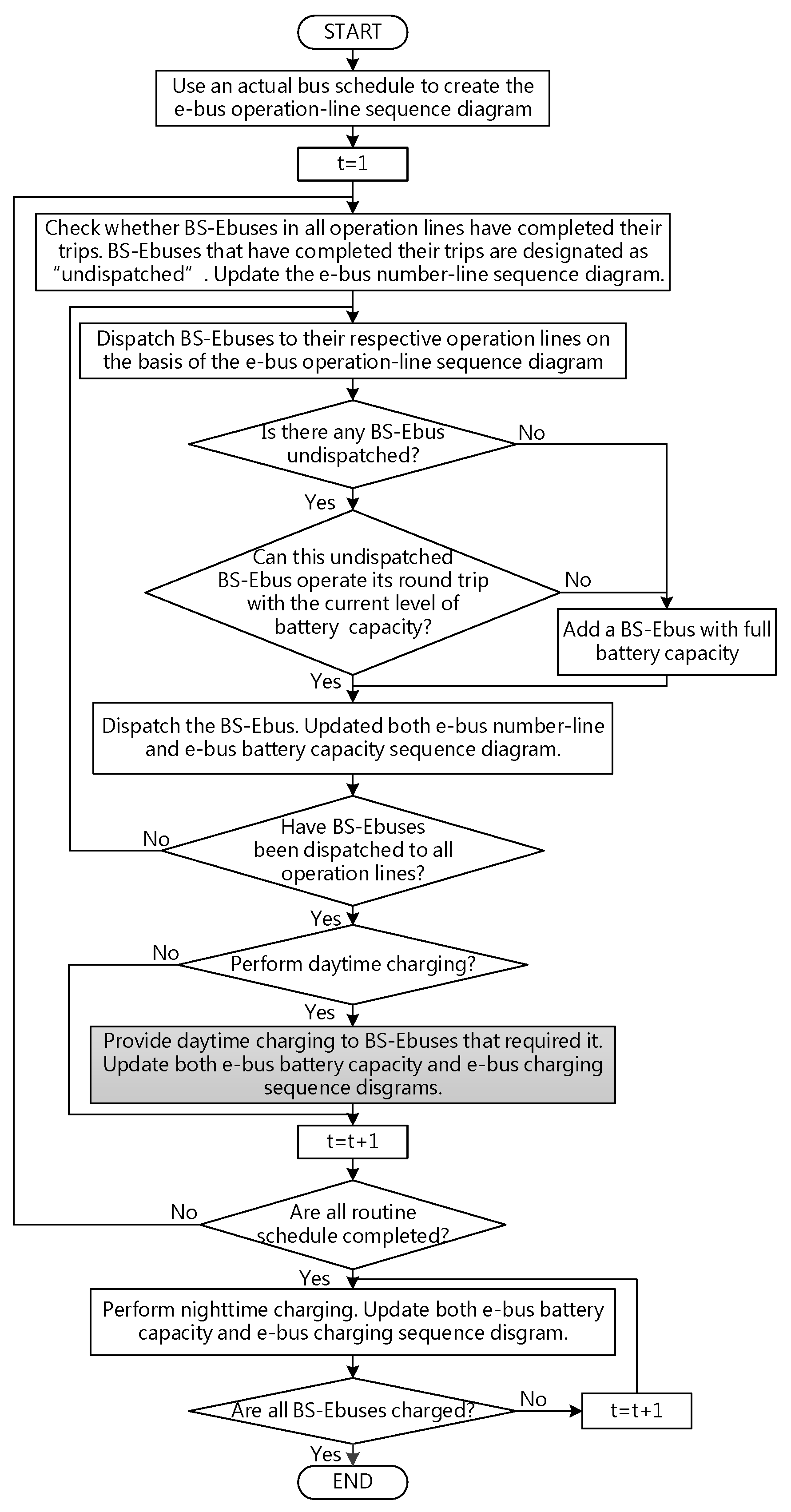
Figure 1 illustrates the flow chart of the BS-Ebus system modeling. Most steps of the BS-Ebus system were similar to those of the PI-Ebus system except for the shadowed rectangle, which was changed to provide daytime charging to the BS-Ebuses that require it as shown in Figure 1 [32].
Figure 2 demonstrates the battery-swapping and -charging processes of the BS-Ebus system.
2.1.1. Battery-Swapping Process
Figure 2 shows the battery-swapping flow chart of the BS-Ebus system. The battery-swapping process required 15 min, and the data for system modeling were updated every 5 min. First, whether a BS-Ebus was still undergoing the battery-swapping process was determined. To reduce the number of back-up batteries required by the system, when a BS-Ebus reached the required time for battery swap, a daytime charged battery (preferred) or a back-up battery replaced the used battery. The replaced battery was then recharged in the charging station, and the bus was returned to the depot for its next dispatch. If the e-bus reached the required time for battery swap, the swap time was updated. Subsequently, if any e-buses in the depot were awaiting battery swap, the waiting time for battery swaps was clocked. The steps were repeated until all the BS-Ebuses that required battery swaps were replaced with new batteries and all the data were updated.
2.1.2. Battery-Charging Process
Figure 3 shows the battery-charging flowchart of the BS-Ebus system. First, the recharging location within the charging station was determined for a replaced battery. Subsequently, the initial charging position in the charging curve was determined according to the RBC of the battery. The BCE was calculated and the RBC record was updated. When the battery reached the assigned BCE, the battery-charging process was complete and the battery was ready for use. The steps were repeated until the charging data of the all recharged batteries were completely updated.
2.2. Calculation of the Construction Costs of a Battery-Swapping Electric-Buses System
This study minimized the construction costs of the PI-Ebus and BS-Ebus systems and compared the two systems. This section describes how the construction costs of the BS-Ebus system were calculated. The construction costs included medium and large e-buses, on-board and back-up batteries, battery-charging and -swapping systems, and electricity. The construction costs of the BS-Ebus system as determined through modeling can be related as follows:
where total construction cost; : e-bus cost; : on-board and back-up battery costs; : battery-charging and -swapping system costs; and : electric energy cost.
The details of each item in Equation (1) are described as follows:
- (1)
- E-bus cost: The BS-Ebus system in this study included two types of e-buses, namely medium- and large- e-buses. The bus cost was calculated by multiplying the number of buses with the price. The number of buses was determined according to the actual number of scheduled buses in the timetable.
- (2)
- On-board and additional battery costs: The minimum battery capacity of the on-board batteries was maintained at ≥20% in this study, and the installation interval of the on-board battery was set at 10% (i.e., possible battery capacities include 30%, 40%, 50%, ..., and 90%). The percentage of both on-board and back-up battery capacities of each bus was calculated to obtain the battery cost. The battery cost can be related as follows:where: : number of large and medium e-buses with different on-board battery capacities; : battery price of large and medium e-buses and : number of extra batteries based on full on-board battery capacity for large and medium e-buses.
- (3)
- Battery-charging and -swapping system cost: The batteries that were replaced during daytime were quickly recharged in the battery-swapping facilities. Each battery-swapping facility could accommodate both medium and large buses and simultaneously recharge four batteries. After all scheduled trips were completed, all on-board and back-up batteries were slow charged during nighttime, and all batteries were fully charged by the following morning before the bus schedule commenced. During the slow-charging process, each charger could simultaneously recharge two buses. The battery-charging and -swapping system costs can be related as follows:where: : number of large e-buses and battery charger unit price; : number of medium e-buses and battery charger unit price; : number of battery-swapping systems and unit price.
- (4)
- Electricity cost: Generally, the electricity rate consists of two parts, the flat and meter rates. To simplify the calculations, only the meter rate was included in this study. The meter rate includes summer and nonsummer prices, and the summer price is divided into peak and off-peak periods. The off-peak period starts at 22:30 and ends at 07:30, and the peak period starts at 07:30 and ends at 22:30. The peak price was applied to the daytime charging in this study, whereas the off-peak price was applied to the nighttime charging.
3. Optimization Methods
This study minimized the construction costs of the BS-Ebus transportation system with an existing timetable and routes. The parameters of the daytime charging scheme, namely residual battery capacity and battery-charging energy every 15 min during daytime peak electricity hours, were used. The combinatorial optimization problem was addressed using three metaheuristic algorithms: PSO, GA, and PSO–GA. The optimization results affected the system configuration, including the number of e-buses, capacity of onboard batteries, number of extra batteries, and facilities for charging.
The metaheuristic algorithms that are direct search methods compensate for the disadvantages of local search methods, such as dependence on the neighborhood structure and easy entrapment in a local optimal solution. The solution increasingly improves with the increasing computation time, but it cannot guarantee convergence to global optimization.
3.1. Optimization Variables
This study minimized the construction costs of an e-bus transport system through combinatorial optimization. We optimized the decision variables in each time interval during daytime charging hours from 06:00 to 18:00. These decision variables directly affected the number of e-buses and chargers, on-board and back-up battery capacities, battery-charging facilities, and electricity cost.
Because the PI-Ebus and BS-Ebus systems featured different construction costs, the decision variables for daytime charging also varied. The decision variables for recharging on-board batteries in the PI-Ebus system were the RBC and BCT of undispatched e-buses every 15 min. After the decision variables were established, the undispatched buses in the depot were inspected every 5 min to determine whether they satisfied the required RBC value. Those that met the requirement were driven to the charging station for fast charging according to the assigned BCT value [34]. The decision variables for recharging on-board batteries in the BS-Ebus system were the RBC and BCE of undispatched e-buses every 15 min. After the decision variables were established, the software package inspected the undispatched buses in the depot every 5 min to determine whether these buses satisfied the required RBC value. Those that met RBC requirements were driven back to the charging station for a battery swap, and the replaced batteries were quickly recharged according to the assigned BCE value. BCT and BCE determined whether the batteries were in the recharging process at the beginning of each 5-min interval, and the previously charged batteries did not alter the values of the decision variables.
The RBC requirement ranged from 30 to 90% of the on-board battery capacity with 10% intervals. The maximum was set at 90% to avoid triggering the charge order on fully charged on-board batteries (i.e., 100% battery capacity), and the minimum was set at 30% to avoid battery depletion before the bus returned from the scheduled trip.
BCT ranged from 5 to 60 min with 5-min intervals. In the daytime fast-charging curve, it took 2 h to charge a battery from 0 to 100% capacity. Because the minimum battery capacity in this study was predetermined at 20%, the battery approached full capacity after being charged for 80 min. Therefore, the maximum BCT was set at 60 min with 5-min intervals.
The BCE requirement ranged from 30 to 100% of the on-board battery capacity with 10% intervals, and this decision variable was used for BS-Ebus optimization. Because the replaced batteries could be recharged independently, the BCT did not affect the number of e-buses. Therefore, BCE was chosen over BCT as the decision variable in the BS-Ebus system. According to the data provided by the e-bus manufacturers, the batteries in the BS-Ebus system in this study were single-module batteries. Other vehicles are designed with multi-module batteries, and these batteries are compatible with the single-module vehicles as long as the total capacity and RBC are the same. The software package in this study used the BCE as the optimized variable in the BS-Ebus system to ensure the applicability of the software in subsequent studies.
The authors previously minimized the construction cost of the PI-Ebus system using a GA [28]. Two algorithms, namely PSO and a PSO–GA, were implemented in this study for optimizing the decision variables of daytime charging in both the PI-Ebus and BS-Ebus systems. The two algorithms are described in the following sections.
3.2. Particle Swarm Optimization
The PSO algorithm is based on swarm intelligence, and features advantages such as fast convergence, relatively few parameters, and suitability for dynamic environments [25,26,27,35,36]. The steps of PSO are described as follows:
3.2.1. Particle Coding and Initialization
The same real numbers were used for encoding in the PSO and GA because, in PSO–GA, the encoded vectors in the PSO-optimized position are also used in the GA. The temporal unit of the optimization has 15-min intervals, and the encoding is expressed in integers.
Each particle determines the initial position vector and the velocity vector before starting to evolve. The number of position vectors is equal to the number of daytime charging periods. The position and velocity vectors represent RBC and BCE, respectively. Each position and velocity vector is generated using a stochastic function, and the encoding method is expressed as follows:
where: : position of the j-th particle in the swarm; : h-th position vector of the j-th particle; : number of optimization time slots; : RBC and BCE codes of the j-th candidate solution in the h-th time slot and : number of particles in the swarm.
where: : velocity of the j-th particle in the swarm; : h-th velocity vector of the j-th particle. The position and velocity vectors of each particle are randomly initialized, and the optimal position of the population is obtained after comparison.
3.2.2. Particle Movement
During particle movement, two random numbers, and , and the inertia weight, , are generated. The new velocity, , is calculated using Equation (6) according to the vectors of the current optimal positions of the particle and population, ( and ). To satisfy the requirements of this study, the new velocity must lie between the minimum and maximum. To accelerate the convergence, the inertia weight, , decreases linearly after each iteration [27]. During the first movement, the previous velocity vectors of all particles, , are reset to zero. The new position vector, , is calculated after the new velocity vector, , is substituted into Equation (7):
where: inertia weight; , : individuality and sociality coefficients; : new value of the h-th velocity vector of the j-th particle; : previous value of the h-th velocity vector of the j-th particle; : new value of the h-th position vector of the j-th particle; : previous value of the h-th position vector of the j-th particle; : best known h-th position vector of the j-th particle; : best known h-th position vector in the swarm.
3.2.3. Update the Best Known Particle
The new construction cost can be calculated after each particle movement, and the calculated result is compared with the best known result. If the new result yields a lower construction cost, it replaces the previous best result as the new best known result. Subsequently, all particles in the swarm are ordered according to the calculated results. The best known particle in the current iteration is compared with the previously best known particle. If the former yields a lower construction cost than the latter does, the former replaces the latter as the best known particle.
3.2.4. End Loop
Steps 2 and 3 are repeated until the error between the mean construction cost in the swarm and the best known construction cost is lower than the assigned value; finally, exit the loop.
3.3. Particle Swarm Optimization–Genetic Algorithm
In this study, by using the PSO-generated initial population with sufficient fitness for the GA, the convergence was effectively accelerated, and the search space was expanded [30,31]. The optimized convergence in case studies revealed that because particles easily found the optimal solution during the early stage of evolution, they frequently moved large distances. When the particles obtained more favorable positions in later stages, they could not find more favorable solutions in the neighborhood, resulting in decreased movement. During the execution of a PSO algorithm, the minimum and mean costs in the swarm do not easily converge to approximations, and the convergence effect was difficult to observe. To avoid being trapped in local optima, this study employed the PSO–GA to increase the opportunities to obtain optimal solutions by expanding the search space in later stages of PSO evolution by using the GA to generate new particles. The flow chart of PSO–GA algorithm was shown in Figure 4.
3.3.1. Early Stage of Optimization
Particles with high fitness are generated during each iteration of PSO optimization, and these particles subsequently join the GA population. When the GA population reaches half of the total population, the optimization process enters the later stage. To conduct the optimization with PSO and GA concurrently, the particle swarms or genetic population of both algorithms were encoded in the same scheme.
3.3.2. Later Stage of Optimization
In this stage, the evolution is conducted using the GA. First, particles with high fitness are selected as half of the initial population, and particles in the other half are randomly generated. The selected and randomly generated genes breed a child population with high fitness. In contrast to PSO, PSO–GA features a wide search space, which effectively reduces the number of iterations during optimization. In this study, several PSO–GA iterations yielded the same results as dozens of GA iterations. Although the computational times of the PSO–GA iterations were slightly longer than those of the GA iterations, the former yielded substantially superior results compared with the latter.
4. Results and Discussion
In this section, the PI-Ebus and BS-Ebus system simulations for the Penghu public bus transportation system with the daytime charging scheme and battery maintenance cost are presented. The minimum construction cost for establishing an e-bus system in Penghu was examined through optimization with the GA, PSO, and PSO–GA algorithms.
4.1. Penghu Bus Transportation System
This study adapted the timetable and related parameters of the Penghu bus transportation system from [32]. In the case of Penghu, Lines Zero West/East and TSGH-PB are loop lines operating medium-sized buses in cities, whereas all nonloop lines operate large-sized buses. All service routes originate or terminate at the Makung terminus, as shown in Figure 5. The distance traveled along route was estimated using the locations of stop stations, and the travel time for each route was estimated according to the timetable.
4.2. Minimization of the Construction Cost of the Battery-Swapping Electric-Busesc System
The main scheduling difference between the BS-Ebus and PI-Ebus systems is the time required for battery charging and swapping. The BS-Ebuses can be dispatched immediately after a fast battery swap, whereas the PI-Ebuses require a long recharge time at the charging station. In the optimization of the daytime charging scheme employed in this study, most PI-Ebuses required >20 min for every daytime recharge, whereas the BS-Ebuses only required 15 min for a battery swap. The short downtime of the BS-Ebus system decreased the vacancy rate of the e-buses and enhanced the efficiency of the system.
During daytime operation, if a BS-Ebus was low on battery, the battery was swapped in the battery-swapping facilities at the charging station. The replaced battery module was either immediately recharged to meet the operational demand or recharged at nighttime for the lower electricity rate. Therefore, the BS-Ebus system incurred higher battery costs than the PI-Ebus system did because it required extra batteries.
In this study, the daytime charging scheme for the replaced battery modules in the BS-Ebus system was optimized. The optimization parameters consisted of the RBCs of e-buses every 15 min from 06:00 to 18:00 and the BCEs of the replaced batteries. The RBC parameter setting in the BS-Ebus system was the same as that in the PI-Ebus system. Because BCE provides flexibility for recharging the replaced batteries, it was selected over BCT as an optimization parameter in the BS-Ebus system. In this study, the maximum RBC was set as 100% capacity of the on-board battery.
The only energy-filling facilities of the PI-Ebus system in this study were the e-bus chargers in the charging station. Each charger could only conduct fast or slow charging on one PI-Ebus at one time. In the BS-Ebus system, the energy-filling facilities consisted of battery-swapping facilities and e-bus chargers. The battery-swapping facilities could perform both battery swapping and charging. In each battery-swapping facility, only one battery-swapping process could be performed at one time; nevertheless, four battery modules could be simultaneously recharged using fast charging. In the BS-Ebus system, each charger could simultaneously recharge two e-buses through slow charging, thereby halving the number of chargers required for the PI-Ebus system. The energy-filling facility cost in the BS-Ebus system was greater than that in the PI-Ebus system. Fast charging was performed during daytime in both systems for improved battery utilization, whereas slow charging was performed at nighttime for prolonged battery life.
According to the data provided by the e-bus manufacturers, the e-buses and chargers in the BS-Ebus system have a life expectancy of approximately 10 years, and the batteries in the BS-Ebus system have a life expectancy of approximately 5 years. The 10-year total cost calculated in this study consisted of e-buses, on-board batteries, back-up batteries, chargers, and electricity costs, as shown in Table 1.
4.2.1. Case 1: No Daytime Charging
Case 1 simulated the BS-Ebus system without incorporating daytime charging. When the RBC of an on-board battery was lower than the assigned value, the e-bus returned to the charging station for battery swapping. The replaced batteries were not recharged until nighttime. Fully-charged batteries were not recharged during daytime, and were deployed to e-buses running routes suitable for their RBC.
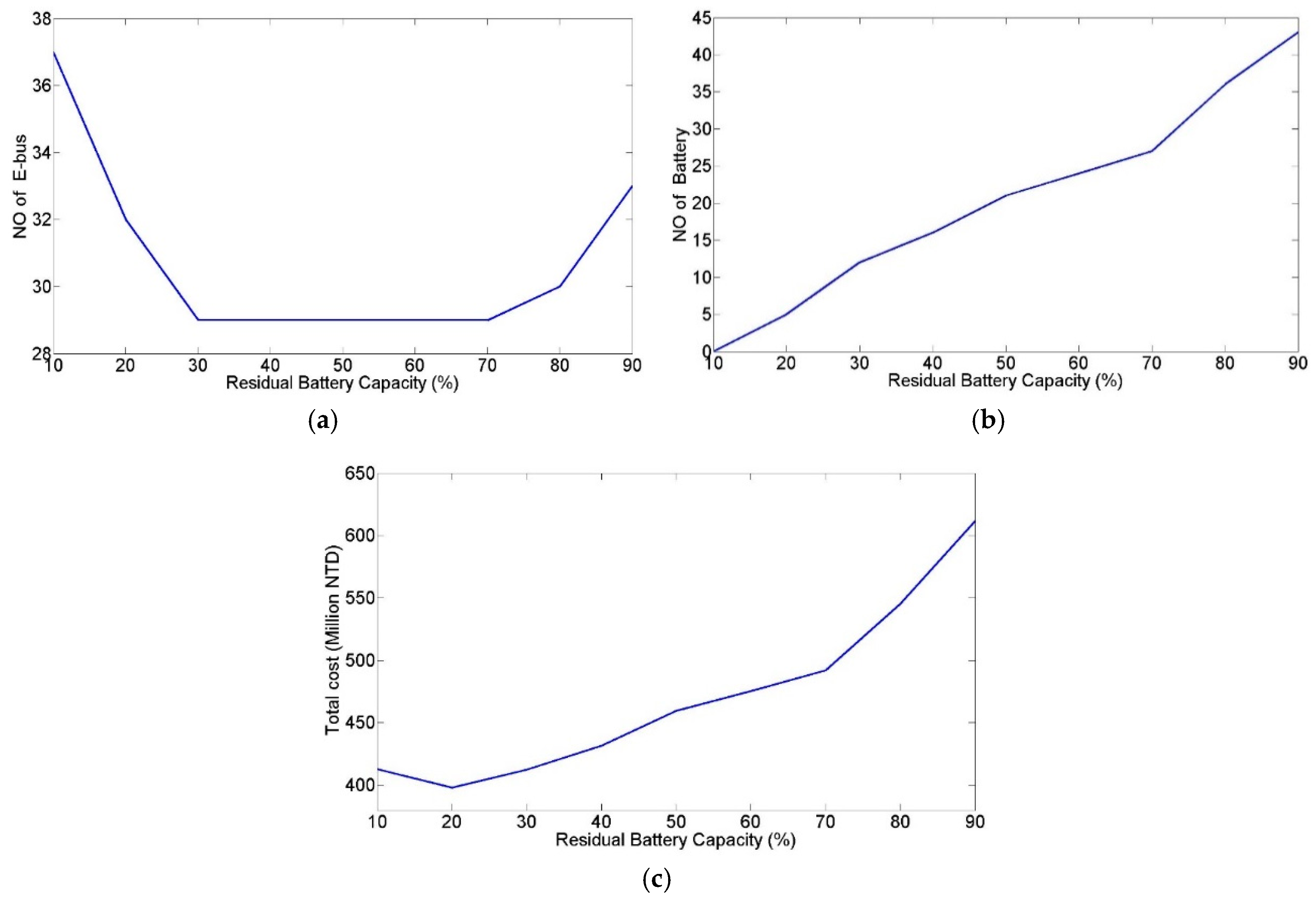
Figure 6a illustrates the number of e-buses plotted against RBC values. When the RBC was lower than 20% and the e-buses were dispatched for long-distance routes, the e-buses remaining in the depot did not have sufficient battery capacity for long-distance routes and their RBCs were not low enough for battery swapping. Therefore, additional e-buses with full battery capacity were required to satisfy the operational demands, which increased the required number of e-buses. However, this problem could be resolved when the assigned RBC value was increased to 30%. When the assigned RBC value exceeded 80%, most e-buses required battery swapping in the charging station after the completion of one trip. The increased number of trips between the depot and charging station led to an increase in the number of e-buses required. Figure 6b illustrates the relationships between different RBCs and the number of additional battery units. The required number of additional battery units increased as the RBC increased because the high RBC increased the frequency of daytime battery swaps. Therefore, additional back-up batteries were required to replace the on-board batteries, resulting in an increased battery cost. Figure 6c demonstrates that the total construction cost increased as the required number of additional batteries increased, except when RBC = 10%. Although the RBC affected the number of e-buses required, the influence was limited.
Table 2 shows the minimized construction cost of the BS-Ebus system without daytime charging. The minimum construction cost occurred when the RBC was set at 20% with 29 large and 3 medium e-buses. When the daily operation commenced, five e-buses were equipped with fully-charged on-board batteries and five additional fully-charged battery modules were required throughout the day. The 10-year construction cost was NT$ 399.9 million.
4.2.2. Case 2: Optimize the Residual Battery Capacity and Battery-Charging Energy by Using the Genetic Algorithm
Case 2 optimized the RBC and BCE every 15 min from 06:00 to 18:00 using the GA. When the RBC of an on-board battery was lower than the assigned value, the e-bus returned to the charging station for battery swapping. Batteries that were replaced earlier in the day and were recharged to the assigned BCE value were the preferred replacement option; batteries that were fully charged at nighttime were selected if the aforementioned batteries were not available, thereby reducing the required number of additional batteries.
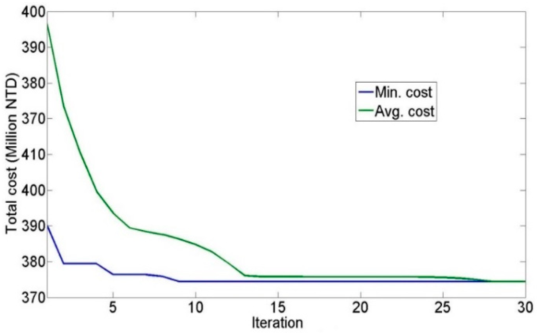
Figure 7 illustrates the optimized convergence in the GA. When the number of iterations reached 30, the error between the mean total cost and minimum total cost was lower than the assigned value, thereby terminating the evolution. Table 3 shows the minimized construction cost optimized by the GA, in which 26 large and 3 medium e-buses and 13 chargers (half of the total number of e-buses) were required. Table 3 lists the battery capacity demands of the two types of e-buses. When the bus operation commenced, the large e-bus fleet consisted of 10 fully-charged e-buses; in addition, the number of e-buses with 90%, 80%, 70%, 60%, 50%, 40%, and 30% charge were two, seven, one, two, two, one, and one, respectively. Moreover, three sets of additional battery modules were required for daily operation. When the bus operation commenced, the number of medium e-buses with 70%, 50%, 30% charge was one, one, and one, respectively. The daily daytime and nighttime BCEs of the large e-bus fleet were 855.8 kWh and 4674.6 kWh, respectively. The medium e-bus fleet operated without additional battery modules, and it consumed 124.80 kWh daily through nighttime charging. The 10-year construction cost was NT$ 372.20 million.
In contrast to Case 1, daytime charging was implemented in Case 2, leading to a reduced on-board battery capacity, two fewer additional battery modules required, and a lower additional battery cost. However, the high electricity cost during peak periods increased the overall electricity cost. In addition, after the 15-min RBC and BCE were optimized using the GA, the increased e-bus occupancy rate led to a decreased number of e-buses required for operation, thereby lowering the e-bus cost. After all the items were aggregated, the construction cost of Case 2 was NT$27.7 million lower than that of Case 1.
4.2.3. Case 3: Optimize the Residual Battery Capacity and Battery-Charging Energy by Using the Particle Swarm Optimization–Genetic Algorithm
Case 3 optimized the RBC and BCE every 15 min from 06:00 to 18:00 by using the PSO–GA. The initial population was trained using PSO. After evolution, the initial population was added to the GA population for optimization. To avoid being trapped in local optima when the evolved population converged, new genes were added to the population for diversity and continuing evolution.
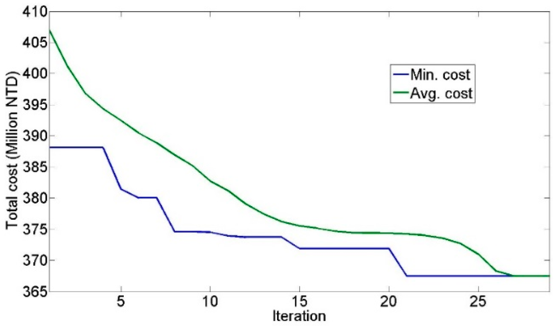
Figure 8 illustrates the optimized convergence in the PSO–GA. When the number of iterations reached 29, the error between the mean total cost and minimum total cost was lower than the assigned value, thereby terminating the evolution. Table 4 shows the minimized construction cost optimized by the PSO–GA, in which 26 large and 3 medium e-buses and 13 chargers (half of the total number of e-buses) were required. Table 4 lists the battery capacity demands of two types of e-buses. When the bus operation commenced, the large e-bus fleet consisted of seven fully-charged e-buses; in addition, the number of e-buses with 90%, 80%, 70%, 60%, 50%, and 40% charge were 3, 10, 1, 1, 1, and 2, respectively. Moreover, three additional battery modules were required for daily operation. When the bus operation commenced, the number of medium e-bus fleet with 70%, 50%, and 30% charge were one, one, and one, respectively. The daily daytime and nighttime BCEs of the large e-bus fleet were 576.4 kWh and 4875.6 kWh, respectively. The medium e-bus fleet operated without additional battery modules, and it consumed 124.80 kWh daily through nighttime charging. The 10-year construction cost was NT$ 367.50 million.
The construction cost for Case 3 was NT$ 4.7 million lower than that of Case 2, and it was the lowest among the three cases in this study. Figure 7 and Figure 8 demonstrate that the GA generated the optimal solution (i.e., the lowest minimum cost) in the 9th iteration, whereas the PSO–GA did so in the 21st iteration. The GA converged faster than the PSO–GA did. After multiple iterations of optimization were conducted, the minimum construction cost in Case 2 converged to approximately NT$ 380 million. The PSO–GA did not converge as fast as the GA did. After multiple optimization iterations, the minimum construction cost in Case 3 converged to approximately NT$ 370 million. Figure 7 and Figure 8 demonstrate the effectiveness of the PSO–GA by revealing that the GA converged to a local optimum.
4.3. Comparission of Battery-Swapping Electric-Buses and Plug-In Electrice-Buses System Results
The authors previously investigated the minimized construction cost of the PI-Ebus system in Penghu [32]. Results of the PI-Ebus and BS-Ebus systems are compared in this section. The different optimization results of the two systems using the GA, PSO, and PSO–GA algorithms are analyzed as follows.
The optimization variables needed to be selected before the construction cost of the e-bus system could be minimized. This study selected the decision variables of daytime charging schemes during a fixed period as the optimization variables. The decision variables in the PI-Ebus system were the 15-min RBC and BCT values of undispatched e-buses, whereas those in the BS-Ebus system were the 15-min RBC and BCE values. The decision variables of the charging schemes directly affected the electricity costs and the numbers of e-buses, chargers, on-board and back-up batteries, and charging facilities.
Table 5 presents the optimized results of the PI-Ebus and BS-Ebus systems according to various algorithms. When daytime charging was not implemented in the PI-Ebus system, all on-board batteries were charged at nighttime for daytime operation. When both daytime and nighttime charging schemes were incorporated into the PI-Ebus system, the decision variables (RBC and BCT) were optimized using the PSO, GA, and PSO–GA algorithms. The results revealed that daytime charging significantly decreased the construction costs of the PI-Ebus system. The optimization results revealed that although the PSO yielded an ineffective result, the GA and PSO–GA algorithms yielded similar results; those of the PSO–GA were slightly more favorable than those of the GA. The GA and PSO–GA yielded the same e-bus and charger costs, indicating that both costs reached the minimum. Therefore, the daytime charging scheme was the key to cost reduction. The GA yielded higher electricity and on-board battery costs than the PSO–GA did, indicating that PSO–GA yielded longer daytime charging hours by comparison. The increased electricity cost in the PSO–GA was offset by the more substantially decreased on-board battery cost. Therefore, the PSO–GA still yielded a lower total cost than the GA did.
In the BS-Ebus system without daytime charging, all on-board batteries were charged at nighttime for daytime operation. When the capacities of these on-board batteries were insufficient, the e-buses were driven to the charging station for battery swapping before subsequent operation. When both daytime and nighttime charging were incorporated into the BS-Ebus system, the decision variables (RBC and BCE) were optimized using the PSO, GA, and PSO–GA algorithms, similarly to the decision variables in the PI-Ebus system. Table 5 demonstrates that the PSO yielded the highest total cost, followed by the GA and PSO–GA. The multiple position vectors of the PSO particles, the discontinuity of the charging scheme corresponding to the construction cost, and the fact that the velocity vectors must be integers contributed to the PSO converging to a local optimum in early iterations (i.e., inability to move to desirable positions). Although the PSO yielded a substantially more favorable result than did the case without daytime charging, the result was not as favorable as that of the GA. When the charging scheme was optimized using the GA, the construction cost was significantly reduced. When the PSO–GA was used, the particles in early iterations were prone to be trapped in local optima. After the inertia was readjusted, particles indicating lower construction costs gradually appeared. Subsequently, the GA evolution in later iterations of the PSO–GA increased the search space of each iteration and yielded more favorable results than the GA did.
Finally, when both the PI-Ebus and BS-Ebus systems were optimized using the PSO–GA algorithm, the e-bus costs in both models were equal. Because additional back-up batteries in the BS-Ebus system required longer nighttime charging hours (and thereby fewer daytime charging hours) than the PI-Ebus system did, the electricity cost in the PI-Ebus system was higher than that in the BS-Ebus system. However, the additional battery and battery-swapping system costs in the BS-Ebus system contributed to a higher total cost than that of the PI-Ebus system. In this study, the daytime charging scheme was optimized using the Penghu public bus transportation system and timetable as an example. The results revealed that the construction cost of the BS-Ebus system was higher than that of the PI-Ebus system. However, the design parameters of the two e-bus systems were provided using different e-bus manufacturers. Although this study strived for consistency, any discrepancy in the parameters may have affected the calculation of construction costs and the optimization results.
5. Conclusions
The 10-year construction costs required for the complete replacement of the diesel buses in the existing transportation system with e-buses were investigated in this study. The PI-Ebus system modeling method was adapted and modified to a BS-Ebus system. The daytime charging scheme was optimized using the PSO, GA, and PSO–GA algorithms. The minimized construction cost of the BS-Ebus system was then compared with the results of the PI-Ebus system.
The utilization rate of the e-buses could be improved when the BS-Ebus system was implemented because of the shorter wait time during daytime charging. However, in contrast to the PI-Ebus system, the battery-swapping system in the BS-Ebus system required more extensive land area and additional batteries.
Three case studies of the BS-Ebus system were conducted for analysis. Daytime charging was not considered in Case 1. When the RBC of an on-board battery was lower than the assigned value, the e-bus returned to a charging station for battery swapping. The replaced batteries were not recharged until nighttime. When the assigned RBCs were excessively low, many e-buses exhibited insufficient battery capacity for long-distance routes. When the assigned RBC was excessively high, the e-buses frequently required battery swaps after completing only one round trip. Both occasions increased the number of e-buses required for daily operations. In addition, the required number of additional batteries increased as the assigned RBC value increased. Because the additional battery cost affected the total construction costs more than the e-bus cost did, the minimum construction cost occurred when RBC = 20%. The 10-year construction cost was NT$ 399.9 million.
Case 2 optimized the RBC and BCE values every 15 min during peak electricity price periods using the GA. In contrast to Case 1, both the on-board battery capacity and the number of additional batteries were reduced when daytime charging was incorporated into the BS-Ebus system. Moreover, the increased utilization rate of e-buses contributed to a NT$ 27.7 million decrease in the total cost. Case 3 optimized the RBC and BCE values every 15 min during peak electricity price periods using the PSO–GA, and the total construction cost was NT$ 4.7 million lower than that of Case 2. The PSO–GA did not converge as fast as the GA did in Case 2, and the early convergence to local optima was alleviated in Case 3. Therefore, Case 3 yielded more favorable results than Case 2 did.
This study compared the PI-Ebus and BS-Ebus systems through the optimization with three algorithms. The multiple position vectors in the PSO particles, the discontinuity of the charging scheme corresponding to the construction cost, and the fact that the velocity vectors must be integers contributed to the PSO converging to local optima in early iterations (i.e., inability to move to desirable positions). In PSO–GA optimization, the PSO conducted the evolution in early iterations. Although the particles may converge to local optima, the GA evolution in later iterations increased the search space at each iteration. Therefore, the PSO–GA yielded more favorable results than the other two algorithms did. The study results also revealed that daytime charging reduced the construction costs of both systems. The PSO–GA yield the lowest construction cost of the three optimization methods for the daytime charging scheme, followed by the GA and PSO algorithms. According to the case studies and parameters provided, the construction cost of the PI-Ebus system was less than that of the BS-Ebus system. Altering the cases or parameters may yield different results. Therefore, the ideal e-bus system must still be determined on the basis of individual cases and parameters.
Acknowledgment
This research was sponsored in part by the Ministry of Science and Technology, Taiwan, under grant MOST 105-2221-E-346-008.
Author Contributions
Shyang-Chyuan Fang and Bwo-Ren Ke conceived and designed the experiments; Bwo-Ren Ke and Chen-Yuan Chung performed the experiments; Shyang-Chyuan Fang and Bwo-Ren Ke analyzed the data; Bwo-Ren Ke and Chen-Yuan Chung contributed analysis tools; Shyang-Chyuan Fang and Bwo-Ren Ke wrote the paper.
Conflicts of Interest
The authors declare no conflict of interest.
References
- Acquaye, A.A.; Duffy, A.P. Input–output analysis of Irish construction sector greenhouse gas emissions. Build Environ. 2010, 45, 784–791. [Google Scholar] [CrossRef]
- Chang, Y.; Ries, R.J.; Wang, Y. The embodied energy and environmental emissions of construction projects in china: An economic input–output LCA model. Energy Policy 2010, 38, 6597–6603. [Google Scholar] [CrossRef]
- Peters, G.P. From production-based to consumption-based national emission inventories. Ecol. Econ. 2008, 65, 13–23. [Google Scholar] [CrossRef]
- Trappey, A.J.C.; Amy, J.C.; Trappey, C.; Hsiao, C.T.; Jerry, J.R.; Chen, L.S.; Kevin, W.P. An evaluation model for low carbon island policy: The case of Taiwan’s green transportation policy. Energy Policy 2012, 45, 510–515. [Google Scholar] [CrossRef]
- Al-Alawi, B.M.; Bradley, T.H. Review of hybrid, plug-in hybrid, and electric vehicle market modeling studies. Renew. Sustain. Energy Rev. 2013, 21, 190–203. [Google Scholar] [CrossRef]
- Sun, F.; Xiong, R. A novel dual-scale cell state-of-charge estimation approach for series-connected battery pack used in electric vehicles. J. Power Sources 2015, 274, 582–594. [Google Scholar] [CrossRef]
- Chen, Z.; Xiong, R.; Wang, C.; Cao, J. An on-line predictive energy management strategy for plug-in hybrid electric vehicles to counter the uncertain prediction of the driving cycle. Appl. Energy 2017, 185, 1663–1672. [Google Scholar] [CrossRef]
- Wang, S.; Shang, L.; Li, Z.; Deng, H.; Li, J. Online dynamic equalization adjustment of high-power lithium-ion battery packs based on the state of balance estimation. Appl. Energy 2016, 166, 44–58. [Google Scholar] [CrossRef]
- Jiang, H.R.; Zhao, T.S.; Liu, M.; Wu, M.C.; Yan, X.H. Two-dimensional SiS as a potential anode material for lithium-based batteries: A first-principles study. J. Power Sources 2016, 331, 391–399. [Google Scholar] [CrossRef]
- Wen, J.; Yu, Y.; Chen, C. A review on lithium-ion batteries safety issues: Existing problems and possible solutions. Mater. Express 2012, 2, 197–212. [Google Scholar] [CrossRef]
- Peng, P.; Jiang, F. Thermal safety of lithium-ion batteries with various cathode materials: A numerical study. Int. J. Heat Mass Transf. 2016, 103, 1008–1016. [Google Scholar] [CrossRef]
- Li, L.; You, S.; Yang, C.; Yan, B.; Song, J.; Chen, Z. Driving-behavior-aware stochastic model predictive control for plug-in hybrid electric buses. Appl. Energy 2016, 162, 868–879. [Google Scholar] [CrossRef]
- Yi, L.; He, H.; Peng, J. Hardware-in-loop simulation for the energy management system development of a plug-in hybrid electric bus. Energy Procedia 2016, 88, 950–956. [Google Scholar] [CrossRef]
- Zhang, S.; Xiong, R.; Cao, J. Battery durability and longevity based power management for plug-in hybrid electric vehicle with hybrid energy storage system. Appl. Energy 2016, 179, 316–328. [Google Scholar] [CrossRef]
- Li, G.; Zhang, J.; He, H. Battery SOC constraint comparison for predictive energy management of plug-in hybrid electric bus. Appl. Energy 2016, 194, 578–587. [Google Scholar] [CrossRef]
- Zhang, X.P.; Rao, R.; Xie, J.; Liang, Y.N. The current dilemma and future path of China’s electric vehicles. Sustainability 2014, 6, 1567–1593. [Google Scholar] [CrossRef]
- García-Villalobos, J.; Zamora, I.; Knezović, K.; Marinelli, M. Multi-objective optimization control of plug-in electric vehicles in low voltage distribution networks. Appl. Energy 2016, 180, 155–168. [Google Scholar] [CrossRef]
- Yan, J.; Xu, G.; Qian, H.; Xu, Y.; Song, Z. Model Predictive Control-Based Fast Charging for Vehicular Batteries. Energies 2011, 4, 1178–1196. [Google Scholar] [CrossRef]
- Rao, R.; Zhang, X.P.; Xie, J.; Ju, L. Optimizing electric vehicle users’ charging behavior in battery swapping mode. Appl. Energy 2015, 155, 547–559. [Google Scholar] [CrossRef]
- Bi, J.; Zhang, T.; Yu, H.; Kang, Y. State-of-health estimation of lithium-ion battery packs in electric vehicles based on genetic resampling particle filter. Appl. Energy 2016, 182, 558–568. [Google Scholar] [CrossRef]
- Blaifi, S.; Moulahoum, S.; Colak, I.; Merrouche, W. An enhanced dynamic model of battery using genetic algorithm suitable for photovoltaic applications. Appl. Energy 2016, 169, 888–898. [Google Scholar] [CrossRef]
- Gen, M.; Cheng, R. Genetic Algorithms and Engineering Design; John Wiley & Sons: New York, NY, USA, 1997. [Google Scholar]
- Montazeri-Gh, M.; Poursamad, A.; Ghalichi, B. Application of genetic algorithm for optimization of control strategy in parallel hybrid electric vehicles. J. Frankl. Inst. 2006, 343, 420–435. [Google Scholar] [CrossRef]
- Mohan, G.; Assadian, F.; Longo, S. An Optimization Framework for Comparative Analysis of Multiple Vehicle Powertrains. Energies 2013, 6, 5507–5537. [Google Scholar] [CrossRef]
- Kennedy, J.; Eberhart, R.C. Empirical study of particle swarm optimization. In Proceedings of the 1999 Congress on Evolutionary Computation, Washington, DC, USA, 6–9 July 1999. [Google Scholar]
- Liu, D.; Wang, Y.; Shen, Y. Electric Vehicle Charging and Discharging Coordination on Distribution Network Using Multi-Objective Particle Swarm Optimization and Fuzzy Decision Making. Energies 2016, 9, 186. [Google Scholar] [CrossRef]
- Kennedy, J.; Eberhart, R.C. Particle swarm optimization. Proc. IEEE. Int. Conf. Neural Netw. 1995, 4, 1942–1948. [Google Scholar]
- Clerc, M.; Kennedy, J. The particle swarm-explosion, stability, and convergence in a multidimensional complex space. IEEE Trans. Evol. Comput. 2002, 6, 58–73. [Google Scholar] [CrossRef]
- Chen, S.Y.; Hung, Y.H.; Wu, C.H.; Huang, S.T. Optimal energy management of a hybrid electric powertrain system using improved particle swarm optimization. Appl. Energy 2015, 160, 132–145. [Google Scholar] [CrossRef]
- Zhang, Q.; Ogren, R.M.; Kong, S.C. A comparative study of biodiesel engine performance optimization using enhanced hybrid PSO–GA and basic GA. Appl. Energy 2016, 165, 676–684. [Google Scholar] [CrossRef]
- Shi, X.H.; Lianga, Y.C.; Leeb, H.P.; Lub, C.; Wanga, L.M. An improved GA and a novel PSO-GA-based hybrid algorithm. Inf. Process Lett. 2005, 93, 255–261. [Google Scholar] [CrossRef]
- Ke, B.R.; Chung, C.Y.; Chen, Y.C. Minimizing the costs of constructing an all plug-in electric bus transportation system: A case study in Penghu. Appl. Energy 2016, 177, 649–660. [Google Scholar] [CrossRef]
- Valdivia-Gonzalez, A.; Zaldívar, D.; Fausto, F.; Camarena, O.; Cuevas, E.; Perez-Cisneros, M. A States of Matter Search-Based Approach for Solving the Problem of Intelligent Power Allocation in Plug-In Hybrid Electric Vehicles. Energies 2017, 10, 92. [Google Scholar] [CrossRef]
- Maigha; Crow, M.L. Economic Scheduling of Residential Plug-In (Hybrid) Electric Vehicle (PHEV) Charging. Energies 2014, 7, 1876–1898. [Google Scholar]
- Yang, Y.; Zhang, W.; Niu, L.; Jiang, J. Coordinated Charging Strategy for Electric Taxis in Temporal and Spatial Scale. Energies 2015, 8, 1256–1272. [Google Scholar] [CrossRef]
- Peng, L.L.; Fan, G.F.; Huang, M.L.; Hong, W.C. Hybridizing DEMD and Quantum PSO with SVR in Electric Load Forecasting. Energies 2016, 9, 221. [Google Scholar] [CrossRef]
Figure 1.
Constructing the battery-swapping e-buses (BS-Ebus) transportation system [32].
Figure 1.
Constructing the battery-swapping e-buses (BS-Ebus) transportation system [32].

Figure 2.
Steps for battery swapping.
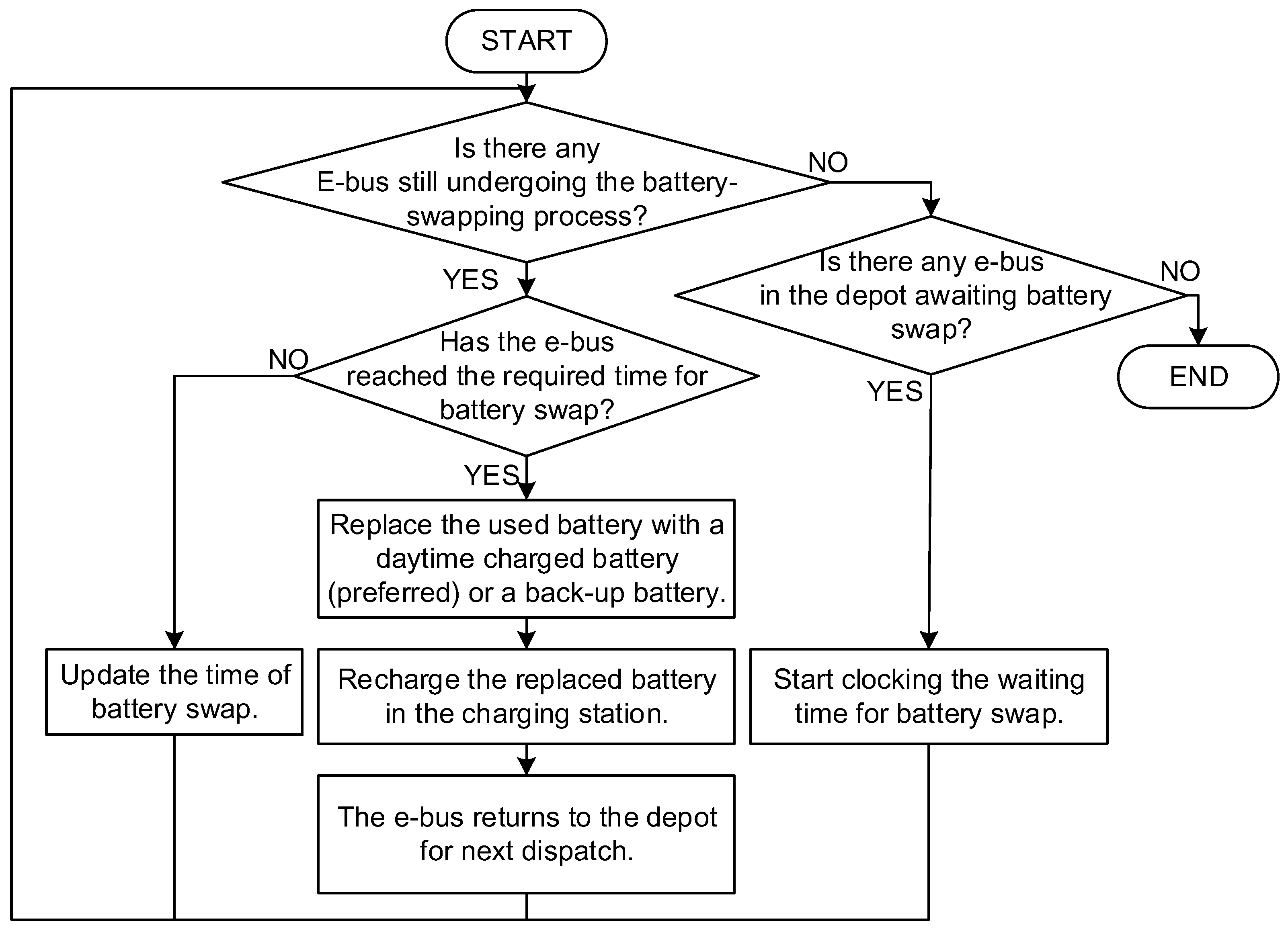
Figure 3.
Steps for battery charging.
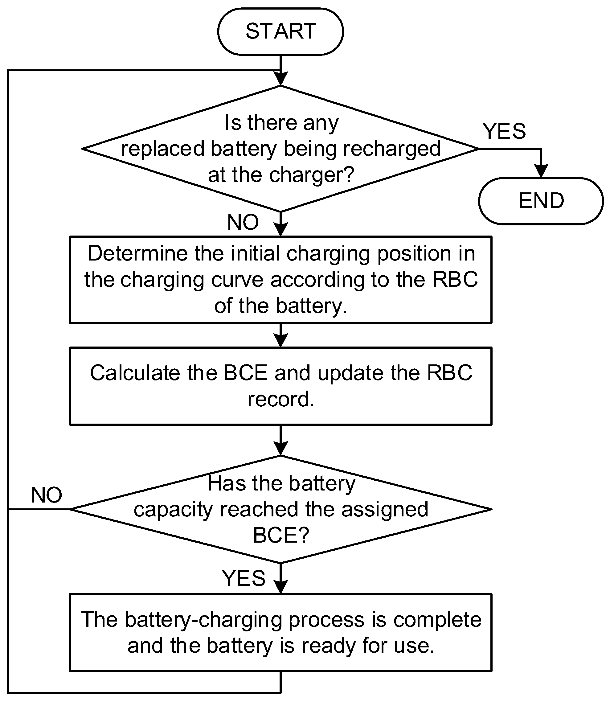
Figure 4.
Flow chart of particle swarm optimization–genetic algorithm (PSO–GA) algorithm application in this study.
Figure 4.
Flow chart of particle swarm optimization–genetic algorithm (PSO–GA) algorithm application in this study.
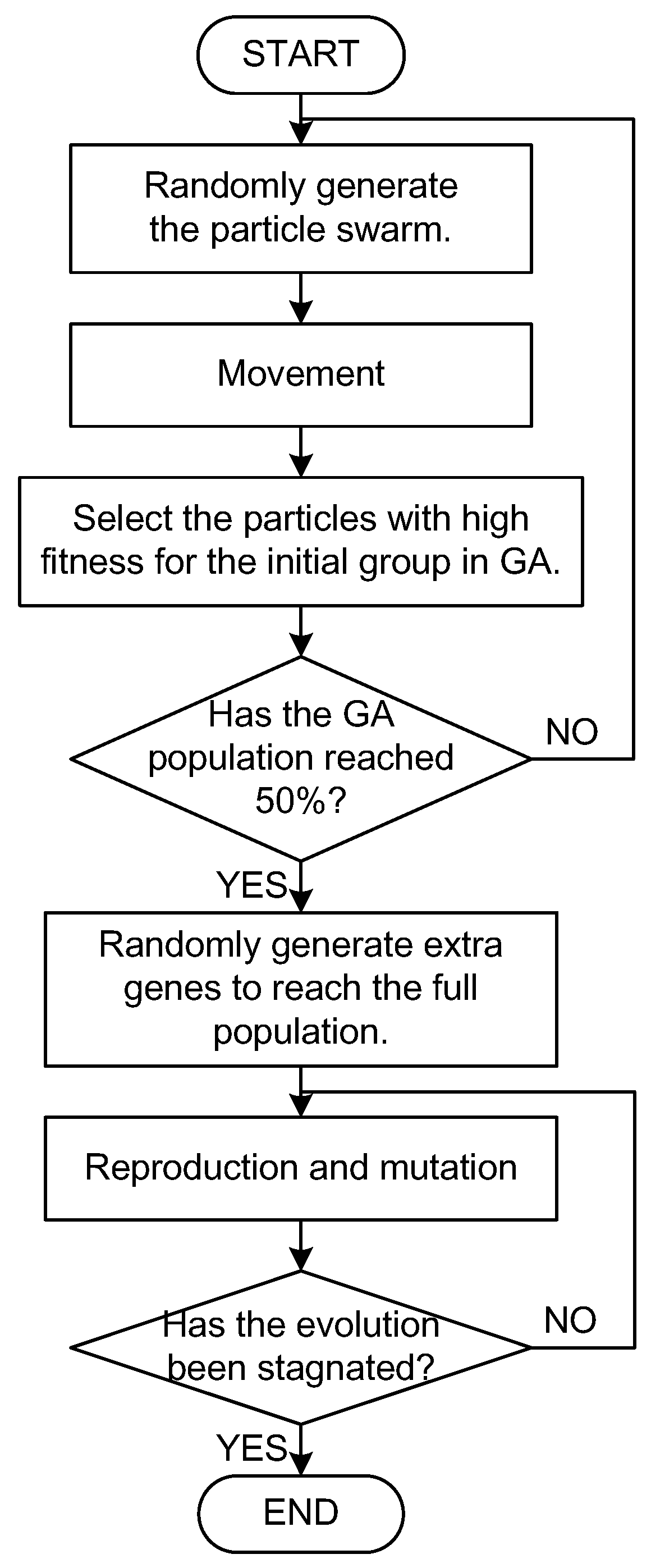
Figure 5.
Penghu bus transportation system [32].
Figure 5.
Penghu bus transportation system [32].
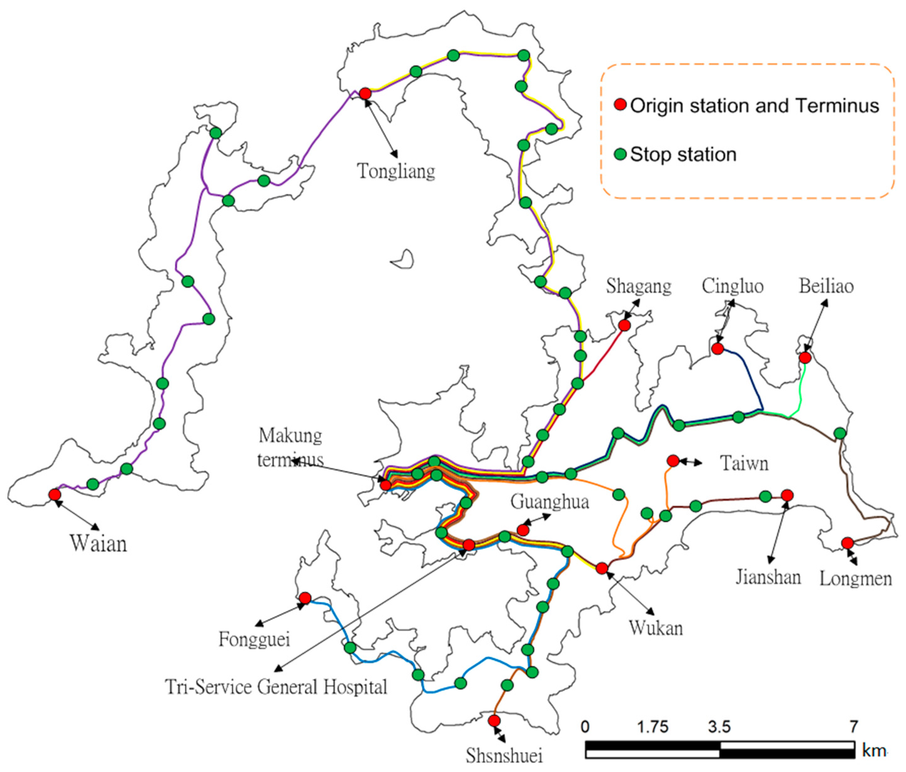
Figure 6.
Results of Case 1. (a) Number of electric-buses (e-buses) for various residual battery capacity (RBCs); (b) number of additional battery units for various RBCs; and (c) construction costs for various RBCs.
Figure 6.
Results of Case 1. (a) Number of electric-buses (e-buses) for various residual battery capacity (RBCs); (b) number of additional battery units for various RBCs; and (c) construction costs for various RBCs.

Figure 7.
Optimized convergence in the GA.

Figure 8.
Optimized convergence in the PSO–GA.

Table 1.
Facility and electricity costs in the battery-swapping e-buses (BS-Ebus) system.
| Price | Bus Type | |
|---|---|---|
| Large | Medium | |
| E-buses (NT$/unit) | 6,000,000 | 4,000,000 |
| On-board batteries (NT$/unit) | 2,600,000 | 1,200,000 |
| Chargers (NT$/unit) | 950,000 | 750,000 |
| Energy-filling facilities (NT$/unit) including battery-swapping equipment and battery chargers | 19,435,000 | |
| Electricity cost (NT$/kWh) | Summer: Peak 3.89 Off-peak 1.99 Nonsummer: Peak 3.79 Off-peak 1.88 | |
Table 2.
Minimized construction costs in the BS-Ebus system without daytime charging. Unit: Million NT$.
Table 2.
Minimized construction costs in the BS-Ebus system without daytime charging. Unit: Million NT$.
| System Construction | Cost Calculation | ||||
|---|---|---|---|---|---|
| E-Bus Type | Large | Medium | Item | 10-Year Cost | |
| On-board battery capacity when dispatched | Full | 5 | 0 | On-board battery cost | 117.8 |
| 90% | 1 | 0 | |||
| 80% | 13 | 0 | |||
| 70% | 5 | 0 | |||
| 60% | 2 | 1 | |||
| 50% | 0 | 1 | |||
| 40% | 1 | 0 | |||
| 30% | 2 | 1 | |||
| Number of e-buses | 29 | 3 | E-bus cost | 186 | |
| Number of extra battery modules | 5 | 0 | Extra battery cost | 26 | |
| Number of chargers | 15 | 2 | Charger cost | 15 | |
| Number of charging facilities | 1 | Facility cost | 19.4 | ||
| Nighttime BCE (kWh) | 5418.6 | 124.8 | Electricity cost | 35.7 | |
| - | Total cost | 399.9 | |||
Table 3.
Minimized construction costs optimized by the genetic algorithm (GA). Unit: Million NT$.
| System Construction | Cost Calculation | ||||
|---|---|---|---|---|---|
| E-Bus Type | Large | Medium | Item | 10-Year Cost | |
| On-board battery capacity when dispatched | Full | 10 | 0 | On-board battery cost | 112.8 |
| 90% | 2 | 0 | |||
| 80% | 7 | 0 | |||
| 70% | 1 | 1 | |||
| 60% | 2 | 0 | |||
| 50% | 2 | 1 | |||
| 40% | 1 | 0 | |||
| 30% | 1 | 1 | |||
| Number of e-buses | 26 | 3 | E-bus cost | 168 | |
| Number of extra battery modules | 3 | 0 | Extra battery cost | 15.6 | |
| Number of chargers | 13 | 2 | Charger cost | 13.9 | |
| Number of charging facilities | 1 | Facility cost | 19.4 | ||
| Daily BCE (kWh) | Day | 855.8 | 0 | Electricity cost | 42.5 |
| Night | 4674.6 | 124.8 | |||
| - | Total cost | 372.2 | |||
Table 4.
Minimized construction costs optimized by the particle swarm optimization–genetic algorithm (PSO–GA). Unit: Million NT$.
Table 4.
Minimized construction costs optimized by the particle swarm optimization–genetic algorithm (PSO–GA). Unit: Million NT$.
| System Construction | Cost Calculation | |||||
|---|---|---|---|---|---|---|
| E-Bus Type | Large | Medium | Item | Decade Cost | ||
| On-board battery capacity when dispatched | Full | 7 | 0 | On-board battery cost | 108.2 | |
| 90% | 3 | 0 | ||||
| 80% | 10 | 0 | ||||
| 70% | 1 | 1 | ||||
| 60% | 1 | 0 | ||||
| 50% | 2 | 1 | ||||
| 40% | 2 | 0 | ||||
| 30% | 0 | 1 | ||||
| Number of e-buses | 26 | 3 | E-bus cost | 168 | ||
| Number of extra battery modules | 3 | 0 | Extra battery cost | 15.6 | ||
| Number of chargers | 13 | 2 | Charger cost | 13.9 | ||
| Number of charging facilities | 1 | Facility cost | 19.4 | |||
| Daily BCE (kWh) | Day | 576.4 | 0 | Electricity cost | 42.5 | |
| Night | 4875.6 | 124.8 | ||||
| - | Total cost | 367.5 | ||||
Table 5.
Optimized results of the plug-in e-buses (PI-Ebus) and BS-Ebus systems according to various algorithms. Unit: Million NT$.
Table 5.
Optimized results of the plug-in e-buses (PI-Ebus) and BS-Ebus systems according to various algorithms. Unit: Million NT$.
| Cost Items | PI-Ebus System | BS-Ebus System | ||||||
|---|---|---|---|---|---|---|---|---|
| Non Day-Charging [32] | Day-Charging | Non Day-Charging | Day-Charging | |||||
| PSO | GA [32] | PSO-GA | PSO | GA | PSO-GA | |||
| E-bus cost | 222 | 174 | 168 | 168 | 186 | 174 | 168 | 168 |
| On-board battery cost | 102.2 | 117.0 | 109.7 | 105.0 | 117.8 | 121.1 | 112.8 | 108.2 |
| Extra battery cost | --- | --- | --- | --- | 26 | 10.4 | 15.6 | 15.6 |
| Charger cost | 29.8 | 23.4 | 22.6 | 22.6 | 15.0 | 14.8 | 13.9 | 13.9 |
| Battery swapping system | --- | --- | --- | --- | 19.4 | 19.4 | 19.4 | 19.4 |
| Energy cost | 38.9 | 58.3 | 50.4 | 53.0 | 35.7 | 41.7 | 42.5 | 42.5 |
| Total cost | 392.9 | 372.7 | 350.7 | 348.7 | 399.9 | 381.5 | 372.2 | 367.5 |
© 2017 by the authors. Licensee MDPI, Basel, Switzerland. This article is an open access article distributed under the terms and conditions of the Creative Commons Attribution (CC BY) license (http://creativecommons.org/licenses/by/4.0/).
Share and Cite
MDPI and ACS Style
Fang, S.-C.; Ke, B.-R.; Chung, C.-Y. Minimization of Construction Costs for an All Battery-Swapping Electric-Bus Transportation System: Comparison with an All Plug-In System. Energies 2017, 10, 890. https://doi.org/10.3390/en10070890
AMA Style
Fang S-C, Ke B-R, Chung C-Y. Minimization of Construction Costs for an All Battery-Swapping Electric-Bus Transportation System: Comparison with an All Plug-In System. Energies. 2017; 10(7):890. https://doi.org/10.3390/en10070890
Chicago/Turabian StyleFang, Shyang-Chyuan, Bwo-Ren Ke, and Chen-Yuan Chung. 2017. "Minimization of Construction Costs for an All Battery-Swapping Electric-Bus Transportation System: Comparison with an All Plug-In System" Energies 10, no. 7: 890. https://doi.org/10.3390/en10070890
Note that from the first issue of 2016, this journal uses article numbers instead of page numbers. See further details here.