
Optimal Power Transmission of Offshore Wind Power Using a VSC-HVdc Interconnection


Electrical Engineering Department, Carlos III University of Madrid, Av. de la Universidad 30, 28911 Leganés, Madrid, Spain
*
Author to whom correspondence should be addressed.
Energies 2017, 10(7), 1046; https://doi.org/10.3390/en10071046
Submission received: 4 April 2017
/
Revised: 6 July 2017
/
Accepted: 17 July 2017
/
Published: 20 July 2017
(This article belongs to the Special Issue Wind Generators Modelling and Control)
Abstract
:High-voltage dc transmission based on voltage-source converter (VSC-HVdc) is quickly increasing its power rating, and it can be the most appropriate link for the connection of offshore wind farms (OWFs) to the grid in many locations. This paper presents a steady-state operation model to calculate the optimal power transmission of an OWF connected to the grid through a VSC-HVdc link. The wind turbines are based on doubly fed induction generators (DFIGs), and a detailed model of the internal OWF grid is considered in the model. The objective of the optimization problem is to maximize the active power output of the OWF, i.e., the reduction of losses, by considering the optimal reactive power allocation while taking into account the restrictions imposed by the available wind power, the reactive power capability of the DFIG, the DC link model, and the operating conditions. Realistic simulations are performed to evaluate the proposed model and to execute optimal operation analyses. The results show the effectiveness of the proposed method and demonstrate the advantages of using the reactive control performed by DFIG to achieve the optimal operation of the VSC-HVdc.
1. Introduction
During 2015, 13,805 MW of wind power was installed across Europe, of which 12,800.2 MW was in the Europe Union (EU). Of the 12,800.2 MW installed in the EU, 9765.7 MW was onshore and 3035.5 MW offshore. In 2015, the annual onshore market decreased in the EU by 7.8%, and offshore installations more than doubled compared to 2014 [1]. This increase in offshore installation is expected to continue in the future. Large offshore wind farms (OWFs), typically between 250 MW and 1000 MW, are likely to be built within a distance of approximately 100 km to 150 km from the coast [2]. These OWFs will have to contribute to the operation of the grid as well as to the grid’s reliability and security.
OWFs must inject their energy into the grid through stronger connection buses at higher voltage levels, and thus they require larger transmission lines. As distances increase (mainly undersea), so do the AC cable costs, and the cost becomes prohibitive beyond certain distances [3]. Long AC cables produce large amounts of capacitive reactive power and thus reduce the transmission capacity. For long distances, high-voltage DC (HVdc) connections are an interesting option, and they are especially adequate for undersea cables. Today, HVdc transmission is based on two alternative technologies, namely, Line Commutated Converters (LCC), using thyristors, and Voltage Source Converters (VSC), using Insulated Gate Bipolar Transistors (IGBTs) [2].
LCC-HVdc links are generally used in high-power applications, typically 1000 MW or higher. However, a LCC-HVdc requires a strong AC voltage system for its commutation and to allow the converters to work properly. Moreover, it cannot provide independent control of the active and reactive powers. Thus, either a synchronous compensator or a Static Synchronous Compensator (STATCOM) is required at the offshore station to supply the necessary short-circuit capacity [3]. VSC-HVdc technology overcomes this deficiency by using auto-commutated switches, and it can feed island and passive networks. Further, reactive power control is independent of the active power control. Thus, VSC-HVdc links are attractive for the connection of OWFs to the grid [4,5,6].
DFIG wind farms and HVdc links have been thoroughly studied as separate components. In [7], an optimized dispatch control strategy for the active and reactive power output of the DFIG was considered for onshore wind farms. Nevertheless, the reactive power capability curve of wind turbines is not considered. The incorporation of the active power-reactive power P-Q wind turbine curve in the Optimal Power Flow (OPF) algorithm is shown in [8,9]. In this instance, the method proposed obtains the set points and takes into consideration the loading capabilities of the wind turbines. The incorporation of the VSC-HVdc equations in the OPF is formulated in [10], which gives suitable algorithms to determine the best solution for high-power systems with VSC-HVdc. In [11,12], the representation of a system consisting of one OWF connected to the grid through a LCC-HVdc link (OWF+HVdc) was proposed. The difficulties with the controllability of a LCC-HVdc link (mainly on the sea side) are highlighted on these papers.
This paper proposes the integrated operation of the OWF and the DC interconnection, including in a unique optimization problem, a VSC-HVdc steady-state model, and the detailed representation of an OWF, aiming to calculate the optimal combined operation. The optimal method considers the doubly fed induction generator (DFIG) capability limits, the HVdc restrictions, and the operational requirements in one unique optimization problem, aiming for the improvement of the overall system operation. The main objective of this operation is to maximize the active power output of the configuration of the DFIG and VSC-HVdc, i.e., to minimize electrical losses throughout the system. The results show the effectiveness of the proposed method and demonstrate the advantage of using the reactive power control performed by DFIG to achieve the optimal operation of the VSC-HVdc.
2. DFIG Base Wind Turbine
The doubly fed induction generator (DFIG), when connected to the grid, can supply power at constant voltage and constant frequency while the rotor speed varies [13]. The DFIG consists of a wound rotor induction generator with the stator directly connected to the grid and with the rotor interfaced through a power electronics converter (back-to-back). This configuration is especially interesting as it allows the power electronic converter to deal with approximately 30% of the generated power, reducing the cost and the efficiency compared with full converter based topologies [14]. Additionally, a DFIG has a decoupled control of active power and reactive power, using vector control techniques.
When DFIG-based wind turbines are connected to a LCC-HVdc transmission, the OWF side is working in islanding mode. Therefore, the DFIG must contribute to the regulation of the grid voltage and frequency, and it operates as a variable speed stand-alone generating system. Several control strategies have been proposed to regulate the generator in this operation mode [15,16,17]. However, a VSC-HVdc can work as a grid-supporting converter by using a control loop [18]. This includes the regulation of the voltage amplitude and frequency in the OWF grid. In this paper, the development of a VSC-HVdc model follows the control strategies of a grid-supporting converter presented in [19].
On the other hand, the capability curve of the DFIG-based wind turbines depends on the stator active power, while the rotor power is related to the stator power through the slip, s [15]. Therefore, the reactive power capability relies on the rotor speed of the wind turbine [9,10]. The total capability of the DFIG can be used to improve the combined operation of the OWF and HVdc system.
Reactive Power Capability Limits
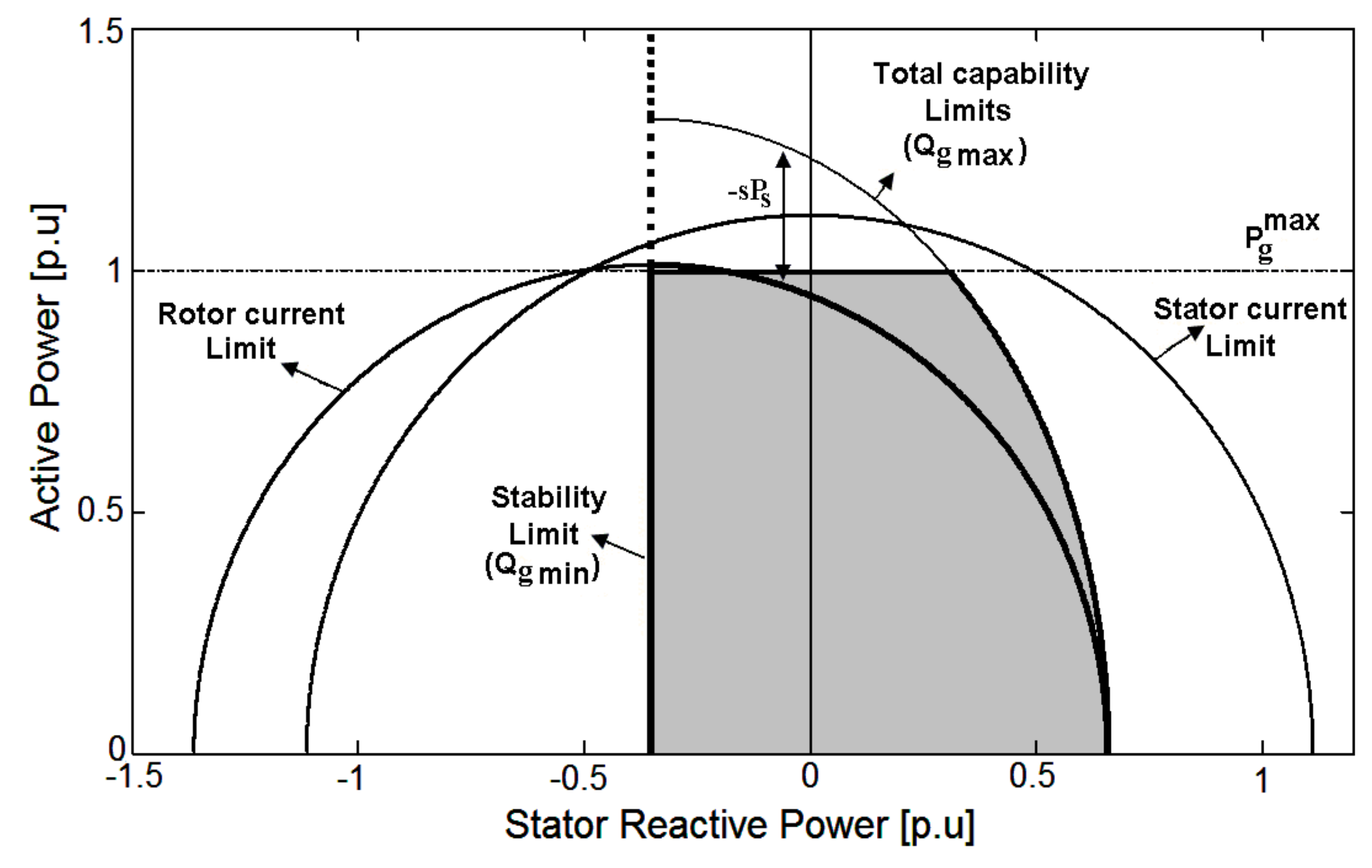
The DFIG reactive power capability limits are obtained by considering both the stator and the rotor rated currents [10]. These currents are responsible for the heating of the stator and the rotor windings due to Joule losses. Another limit of the wind turbine is the maximum active power due to the aerodynamics power (Pgmax), which results from the available wind speed and the power conversion curve. In Figure 1, the steady-state capacity limits of the DFIG are represented, including the stability limit of the generator [11,12]. The resulting P-Q curve is formed by the minimum absolute value of the four operational limits (the stator current, the rotor current, the maximum active power, and the stability limit). The shaded area in Figure 1 represents the feasible area of operation for the DFIG-based wind turbine.
A variation in the stator voltage affects the capability limits of the DFIG (without including Pgmax). Moreover, the rotor limit depends on the rotor winding rating of the DFIG and the rating of the power converter. However, the power converter must be rated to at least the rated current of the rotor winding, while the rotor voltage is related to the stator voltage through the slip [12].
In conventional operation, the active power generated by the DFIG has a given value that depends on the wind speed and the power curve of the turbine. However, the DFIG reactive power can be controlled between the limits shown in Figure 1. These reactive power limits can be expressed as [11]:
where , , and Us is the stator voltage.
To maintain the simplicity of the model, the DFIG parameters (magnetising reactance XM and stator reactance Xs) and the rated rotor current are assumed to be constant values for all the feasible operation points [12].
3. VSC-HVDC Steady State Model
The steady-state model of the VSC-HVdc can be ideally simplified with the following assumptions [20]:
- The internal voltages have constant amplitude and frequency, and they are balanced.
- All voltages and currents harmonically produced by the converters are neglected.
- The internal losses of the converters are neglected, i.e., the valves are considered ideal, that is, without a voltage drop.
- The DC current and voltage have no ripple.
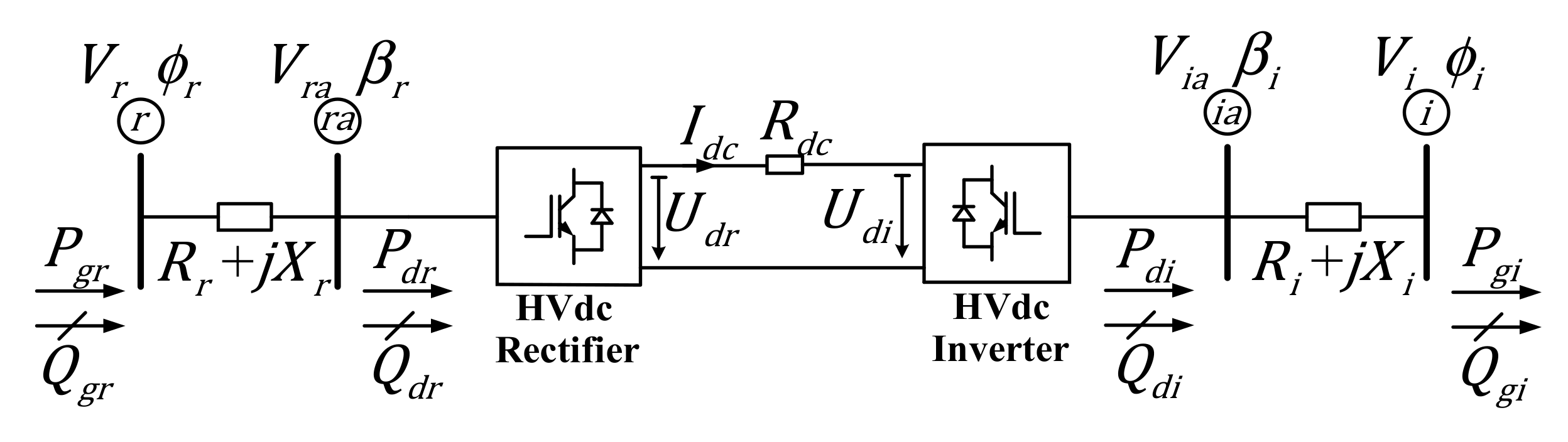
The VSC-HVdc link consists of two voltage-source converter stations (VSC) with series-connected Insulated Gate Bipolar Transistor (IGBT) valves controlled by Pulse Width Modulation (PWM). The OWF side converter operates as a rectifier and the other as an inverter. The two converters are joined together by a DC cable, as represented in Figure 2.
The operation principles of the VSC-HVdc can be explained by considering each VSC station separately. In Figure 2, one VSC is connected to the OWF side and the other to the grid, both using an interfacing transformer. The impedances of the interface transformer are Rr + jXr and Ri + jXi. The amplitude and the phase angle of the output fundamental AC voltage (Vra < βr and Via < βi) for each VSC station can be modified with respect to the amplitude and the phase angle of the respective AC system voltage (on the OWF side, Vr < φr, and on the grid side, Vi < φi) [4]. The amplitude and the phase angle of the voltage drop across the impedances of the interfacing transformers are modified with the active and reactive power flows. Finally, the active power flowing through the HVdc link can be calculated knowing the DC voltage at each HVdc side, Udr and Udi, respectively, together with the DC current Idc. In this work, all magnitudes are in per unit (p.u.) for both AC and DC grids. The relationship between the AC and DC base values is included in Appendix A.
3.1. Rectifier Model
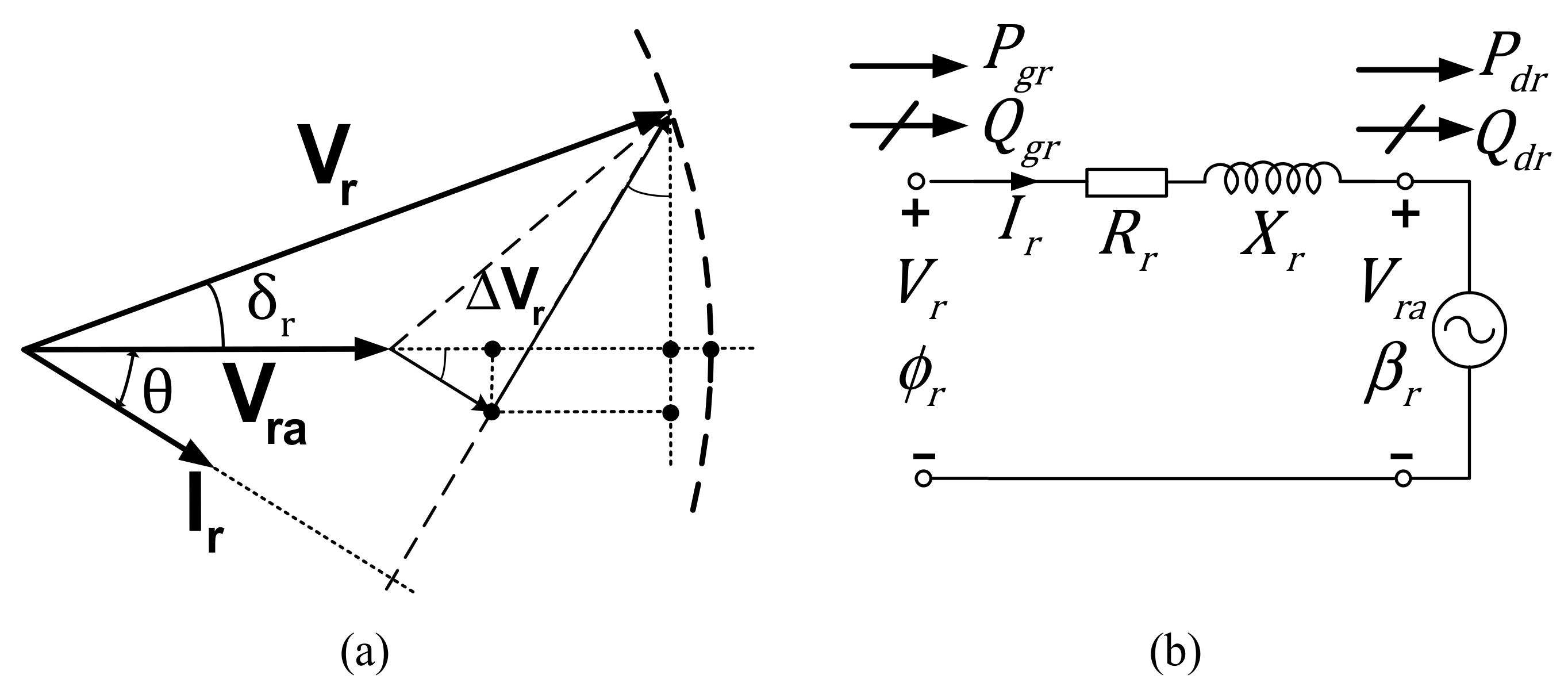
Based on the equivalent circuit represented in Figure 2, it is possible to obtain the equations that model the rectifier operation when it is connected to the OWF (Figure 3). It must be stressed that, in the present operation, the active power flow is always from the OWF to the external grid, which simplifies the operational modes of the HVdc.
The VSC output fundamental AC voltage phasor Vra lags the AC voltage phasor Vr by an angle δr (see Figure 3) because the active power Pgr flows from the OWF to the rectifier. Therefore, the active power flowing into the HVdc link Pdr will modify the phase shift angle δr. This angle is defined as:
However, the reactive power Qgr flows from the OWF to the rectifier when the amplitude of the AC voltage phasor Vr is larger than the VSC output fundamental AC voltage phasor Vra for a relatively small δr. Therefore, the reactive power supplied or absorbed, Qdr, by the rectifier is modified by adjusting the amplitudes of the VSC output fundamental AC voltage (Vra).
The VSC output fundamental AC voltage magnitude at the rectifier terminal, Vra, is related to the amplitude modulation index of the space-vector PWM [17], Mr (p.u.), and to the DC voltage Udr by:
The active power, Pdr, flowing into the DC side of the rectifier can be expressed as follows:
By taking into consideration the voltage drop ΔVr given in Figure 3, according to the phasor representation, the equivalent circuit, and (4) and (5), the reactive power flowing into the AC rectifier terminals Qdr can be calculated as follows [20]:
where .
Similarly, the angle δr may be calculated using the following equation:
Additionally, the active and reactive powers, Pgr and Qgr, can be obtained with the following expressions:
3.2. Inverter Model
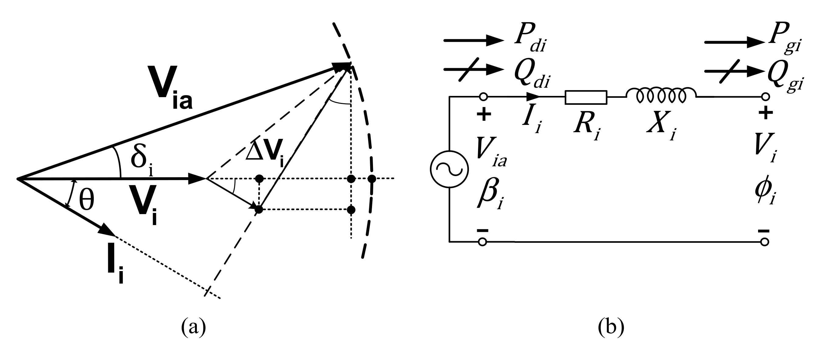
Similar to the rectifier operation mode and based on the equivalent circuit shown in Figure 4, the inverter operation mode of the VSC station connected to the grid can be obtained.
The phasor VSC output fundamental AC voltage Via leads the phasor AC voltage Vi by an angle δi (see Figure 4) when the active power Pdi flows from the AC side converter to the grid. This angle is defined as:
The reactive power Qdi flows from the AC side inverter to the grid when the amplitude of the phasor VSC output fundamental AC voltage Via is greater than the phasor AC voltage Vi for a relatively small δi.
Similar to the rectifier mode operation of the VSC, the DC voltage Udi can be calculated as:
where Mi (p.u.) is the amplitude modulation index at the inverter station.
The active and reactive powers, Pdi and Qdi, of the AC side inverter can be expressed as follows:
The active power Pgi can be obtained by:
The angle δi may be calculated as:
Finally, based on Figure 2, the current flow through the DC link between the two terminals of the converter is expressed by (17). The equivalent model the HVdc link is modeled as a cable with a resistance Rdc.
4. Optimization Procedure
This paper focuses on the maximization of the active power output of the OWF+VSC-HVdc, given the restrictions imposed by available wind power, the reactive power capability of the DFIGs, and the VSC-HVdc link models. The best operation point can be found through an optimization problem involving the AC and DC grids, the interface between these grids, and a wind turbine representation.
The general optimization problem can be formulated as:
where Pgi is the active power output of the OWF+VSC-HVdc system, X is the vector of optimization variables for the combined ac-dc OWF+VSC-HVdc system, h(X) are the equality constraints of the AC and DC grid equations, and g(X) are the inequality constraints.
4.1. Optimization Variables
The optimization variable vector is defined as:
where
is the vector of the voltage magnitudes for each AC bus in the OWF+VSC-HVdc system and n is number of AC buses in the system (including the output bus, i.e., the connection with the external system),
is the vector of phase angles for each AC bus voltage in the OWF+VSC-HVdc system,
is the vector of the reactive power generations for all of the DFIGs at the AC buses, including the grid bus, and
is the vector of the HVdc link variables.
In this analysis, all of the variables are continuous, and the dimension of the optimization variable vector is (2n + ng + 10), where ng is the number of AC generator buses in the wind farm plus the output bus.
4.2. Equality Constraints
The balances between the active and reactive powers at the AC buses of the OWF are represented by equality constraints. For each k AC bus (except those connect to the HVdc link), the nodal power flow equations are given by:
where Gkj and Bkj are the conductance and susceptance, respectively, of the transmission lines and the transformers between the k and j buses of the OWF, Pgk and Qgk are the active and reactive power generations for each DFIG, respectively, and δkj is the phase angle difference between the k and j buses.
The active and reactive balances in AC bus k (when connected to the VSC-HVdc link) must consider the DC power flowing into the DC terminals. Moreover, the incorporation of passive filters connected to both the HVdc rectifier and the inverter terminals, represented by constant shunt admittances Ys, must be also included in the reactive power balances (although this value is small for the VSC-HVdc links, and it can generally be ignored). Therefore, the equations for the active and reactive power balances at the AC bus r (see Figure 2) on the rectifier converter side are:
The equations for the active and reactive power balances at the AC bus ia (see Figure 2) can be written as:
The equations of the HVdc model (see Section 3) are explicitly modeled as equality constraints by the following equations:
In this formulation, the optimization problem includes (2n + 12) equality restrictions.
4.3. Inequality Constraints
The voltage and phase angle limits for AC buses are represented as an inequality constraint in the model:
The active power limit in each DFIG wind turbine is represented as:
The capability limits in each DFIG wind turbine set of the OWF are represented as:
The reactive generation limit for the output bus is represented as:
The operational limits in the HVdc model of vector Xhvdc are given by:
where the additional subscripts r and i are used to denote the quantities of the rectifier and inverter sides, respectively. Moreover, Tik max and Tik are the maximum limit and the variable value of the apparent power of the transmission line between buses i and k, respectively.
The optimization problem considered here requires the representation of [2(2n + 2ng + 9)] inequality constraints. This paper solves the proposed optimization problem using the Predictor-Corrector Primal-Dual Interior Point method, as described in [21].
5. Case Study
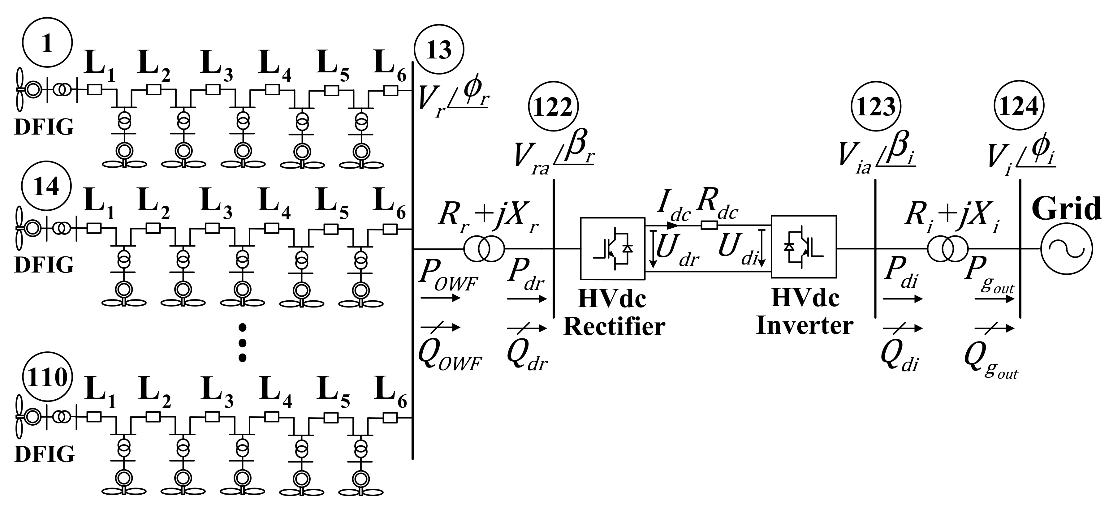
To illustrate the optimization procedure, an OWF comprised of 60 × 5 MW DFIG-based wind turbines (resulting in a 300 MW OWF) is connected to a VSC-HVdc transmission link and, subsequently, to the grid. The string cluster is composed of six DFIG wind turbines with step-up transformers operated at 690 V/30 kV and 5 MVA and an impedance transformer equal to Xtr = 0.05 p.u. and Rtr = 0.005 p.u. (the base values are the generator rating), as shown in Figure 5. The submarine cable parameters are shown in Table 1 [22]. The AC bases are Vac_base = 132 kV and Sbase = 300 MVA. The DC bases are defined by using the equations in Appendix A.
The VSC-HVdc link has a rating of 300 MW and operates at ±100 kV. Each converter has a 30 kV/132 kV step-up transformer with an impedance equal to Rr,i = 0.0065 p.u. and Xr,i = 0.1 p.u. The total resistance of the HVdc cable is Rdc = 0.9 Ω (0.067 p.u.) for a length of 100 km.
To simulate the performance of the model for all operational wind speeds, the case study was sequentially solved for different operation points. Each wind turbine power input, Pgk, was varied between 0.0833 MW (0.00027 p.u.) and 5 MW (0.0167 p.u.), with a step size of 0.0833 MW (0.00027 p.u.). The allowable ranges of values for all variables are given in Table 2 and Table 3.
5.1. Non-Optimal Operation of the OWF-VSC-HVDC
For comparison with the proposed optimization procedure, a power flow solution is used to find the steady-state operating point of the VSC-HVdc and OWF system without optimization.
In this OWF study case, the control of the rectifier station is modeled as the slack node (i.e., bus 122 in Figure 5 has a constant voltage module, Vra = 0.97, with a phase angle βr = 0°). This control approach of the rectifier is very useful because the power flow problem involves fixing a reference angle and balancing the active and reactive power in the internal grid of the OWF.
Moreover, the reference AC bus at the inverter side, named the 124-bus (see Figure 5), has the values Vi = 1.0 and βi = 0°. Consequently, the modulation indexes at the converters are constants in the model of the VSC-HVdc (Mr = 0.87 and Mi = 0.9 for the fixed reference AC voltages). Furthermore, each wind turbine bus on the OWF is expressed in terms of the active and reactive powers supplied (PQ bus). Hence, each DFIG must have a particular power factor (pf) based on the Pgk range.
These fixed values ensure that the solution of the power flow problem fits the allowable range of values for the AC and DC voltages (see Table 2 and Table 3).
Figure 6a illustrates the active and reactive power on all DFIGs of the first row of the OWF under a predetermined power factor (pf = 0.9 leading) at different wind speeds.
Figure 6b shows that the generator voltage modules of the first row of the OWF are increased due to the injection of reactive power in those buses. However, this reactive power injection (in Figure 6d) causes an increase in the voltage at the collector bus (13-bus, see Figure 5), as shown in Figure 6c.
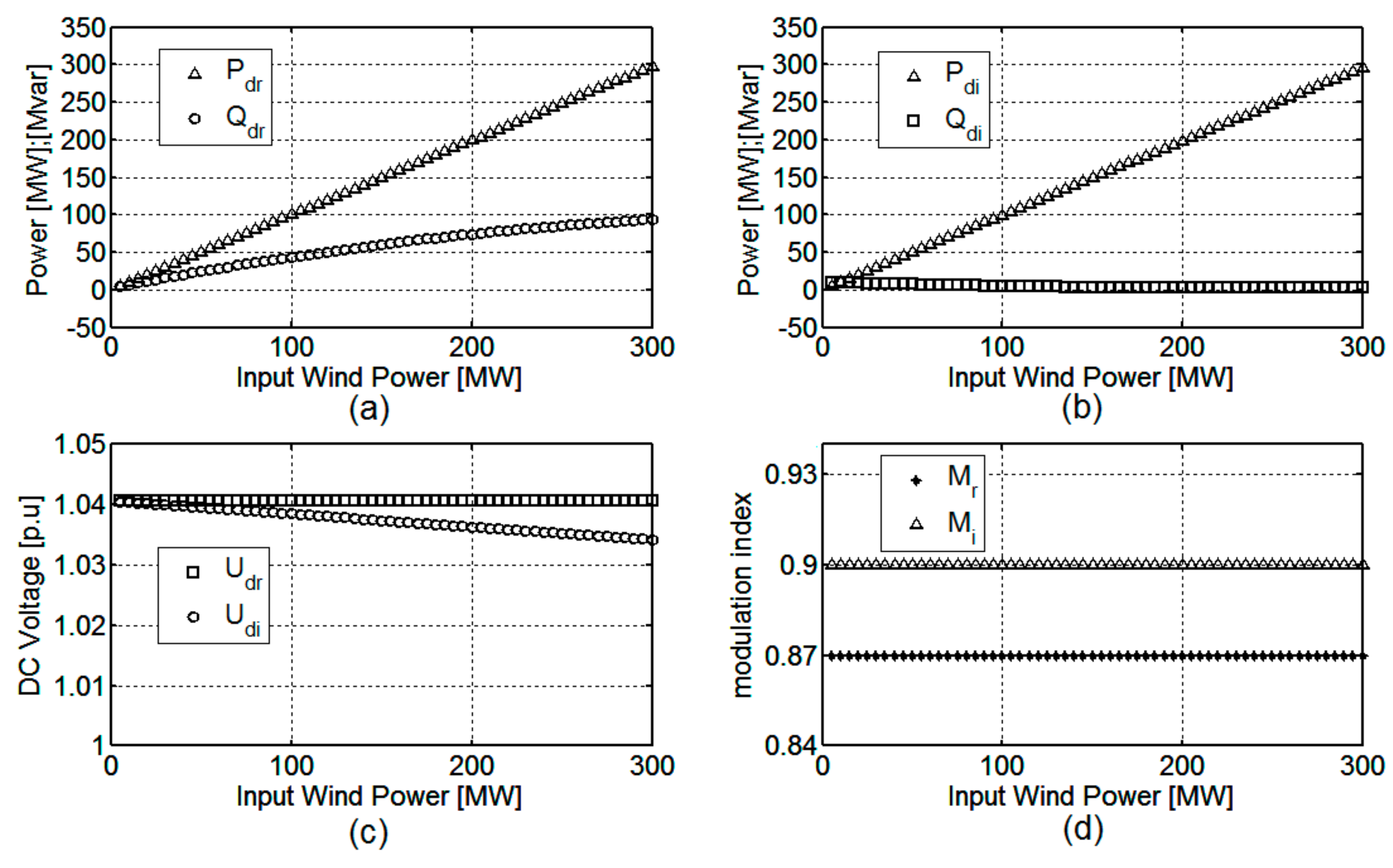
Figure 7 shows the variables of the VSC-HVdc model. In Figure 7a, the reactive power absorbed by the rectifier station (Qdr) causes the rectifier to operate with a low power factor for a full load due to the injection of reactive power by the DFIGs of the OWF. However, the inverter station almost maintains a unity power factor over all ranges of values, as is observed in Figure 7b.
As expected, the DC voltage on the rectifier (Figure 7c) is constant for all ranges of operation due to the fixed modulation index (Mr). The fixed modulation indexes at the converters of the VSC-HVdc are shown in Figure 7d. The selected values (Mr = 0.87 and Mi = 0.9) fulfill two requirements for the safe operation of the system; the first value achieves the allowable range of values in the AC and DC voltages, and the second value prevents overmodulation in transient operation.
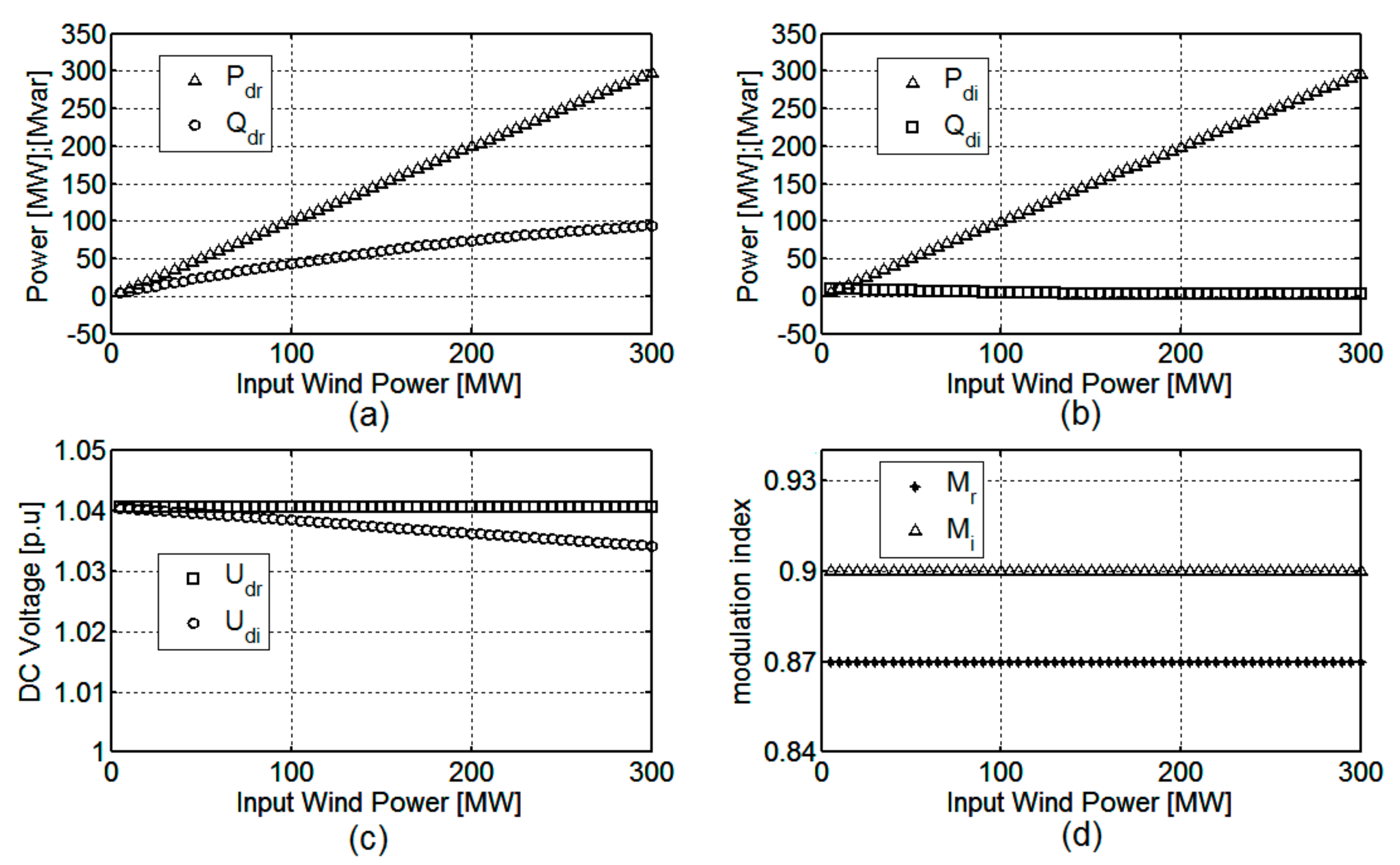
Now, a new non-optimal operation case is considered, where the DFIGs work with a unity power factor, as shown in Figure 8a.
When a power factor equal to one is used, the behavior of the OWF and VSC-HVdc changes slightly. The voltage modules of the first row of the OWF and the collector bus (13-bus) are lower than in the previous case (Figure 8b,c). The reactive power is now supplied by the VSC-HVdc, as shown Figure 8d. This reactive power cannot maintain the voltages in the OWF. Moreover, the reactive power supplied by rectifier station (Qdr) is 48 Mvar with a full load (Figure 9a); therefore, the rectifier is still operating with a poor power factor.
5.2. Optimal Operation of the OWF-VSC-HVDC
This section presents the result of the optimal operation. It is remarkable that there is no need to define PV, PQ, or the reference bus in the optimization procedure. In fact, the voltage can change in all the buses between the specified limits to achieve optimization. However, to assess and compare the optimization approach with the previous case, some variables are predefined in the optimization procedure. Hence, the value of the phase angle of the output fundamental AC voltage at the rectifier (122-bus, see Figure 5) βr is fixed to zero. On the inverter side, the reference bus is the same as in the previous case (Vi = 1.0, and βi = 0°).
The optimization procedure finds the optimal operation using the reactive capability of the DFIG. Figure 10 shows the optimization results. In Figure 10a, the reactive power is fixed in each DFIG to achieve the objective function, i.e., to minimize the power losses in the overall OWF-HVdc system.
Some wind turbines have lagging and leading power factors that are different from those in previous cases. Moreover, the reactive power in the OWF (Figure 10d) is smaller than the value obtained in the previous cases (see Figure 6 and Figure 8), and the voltages of the first row of the OWF and the collector bus (13-bus) are close to one (Figure 10b,c, respectively).
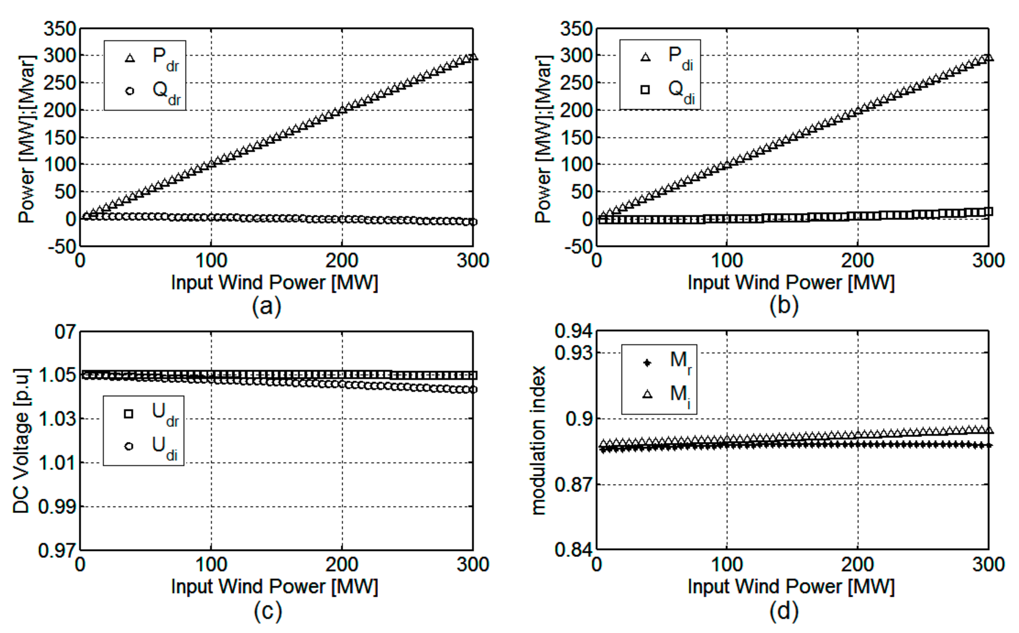
Figure 11a shows that the reactive power delivered by the rectifier is lower than in the previous cases (5 Mvar at full load). Thus, the rectifier operates with a better power factor, and the sizing of the rectifier station may be reduced, which allows the selection of a more efficient, reliable, and cost-effective converter for the VSC-HVdc.
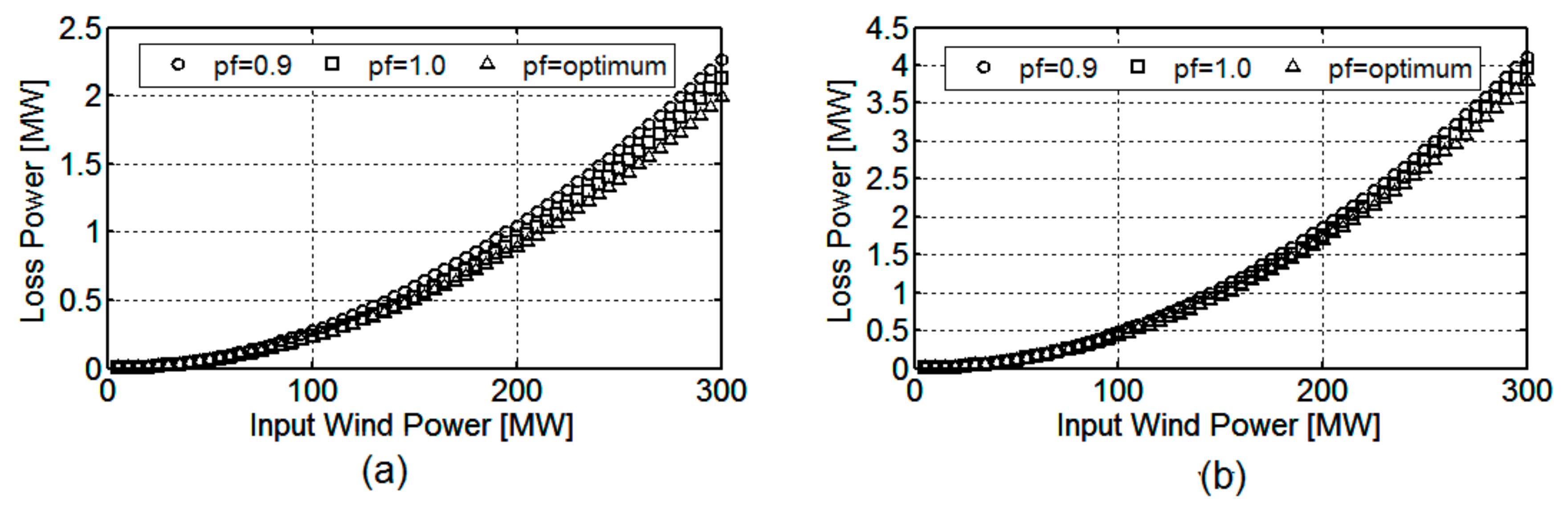
Figure 11c,d show the DC voltage at the VSC-HVdc and the modulation indexes. These values are set to the optimal values to minimize the losses at the HVdc link. Finally, Figure 12 shows the power losses at both the OWF and OWF+VSC-HVdc links. In both cases, losses are reduced when the optimal operation is employed versus operation at a fixed power factor. In the optimal operation, the power factor is set independently at each wind turbine in order to minimize losses.
6. Conclusions
An OWF with a DFIG and a VSC-HVdc link has been modeled to obtain the optimal operation of the overall system. The problem has been formulated as a nonlinear optimization problem in steady state. A case study for a 300 MW-rated OWF was sequentially solved for the whole active power range by taking 60 operation points. The proposed procedure includes the DFIG capability limits, the VSC-HVdc restrictions, and the operational requirements for the right level of security for the OWF-HVdc system. Three different reactive power control concepts for each WT were considered (pf = 0.9; pf = 1.0; and pf = optimum). The proposed optimal method was compared with the solutions of classical power flows, obtained by operating the WT at a constant power factor (pf = 0.9 and pf = 1.0). The simulation results show that optimal operation of the OWF with a VSC-HVdc link can be achieved, allowing a more efficient, reliable, and cost effective converter for the VSC-HVdc link for all wind conditions. These results show, in 300 MW, that the optimization procedure contributes to a reduction in power losses at the OWF of around 13% in the pf = 0.9 case and up to 4.76% for the pf = 1.0 case. The optimization procedure makes use of the reactive capability of the DFIGs to obtain the optimal operation of the combined OWF and HVdc system. The results also show that operation at a fixed power factor in the DFIGs is not an optimal solution.
Acknowledgments
This work has been supported by the I+D program for Research Groups of the Autonomous Community of Madrid under ref. S2013/ICE-2933.
Author Contributions
The authors contributed equally to this work.
Conflicts of Interest
The authors declare no conflict of interest.
Appendix A
Per unit system
A common base power, Sbase, is chosen for both the AC and DC systems. For the DC base quantities:
References
- Wind in Power 2015 European Statistic. The European Wind Energy Association EWEA Report. 2015. Available online: http://www.ewea.org/fileadmin/ewea_documents (accessed on 7 February 2017).
- Bresesti, P.; Kling, W.L.; Hendriks, R.L.; Vailati, R. HVDC Connection of Offshore Wind Farms to the Transmission System. IEEE Trans. Energy Convers. 2007, 1, 37–43. [Google Scholar]
- Ackermann, T. Wind Power in Power Systems; John Wiley & Sons: Chichester, England, UK, 2005; pp. 480–504. [Google Scholar]
- Flourentzou, N.; Agelidis, V.G.; Demetriades, G.D. VSC-Based HVDC Power Transmission Systems: An Overview. IEEE Trans. Power Electron. 2009, 24, 592–602. [Google Scholar] [CrossRef]
- Theologi, A.M.; Ndresko, M.; Rueda, J.L.; Van der Meijden, M.A.; González-Longatt, F. Optimal Management of Reactive Power Sources in Far-offshore Wind Power Plants. In Proceedings of the IEEE Manchester Power Tech, Manchester, UK, 18–22 June 2017. [Google Scholar]
- Kunjumuhammed, L.P.; Pal, B.C.; Gupta, R.; Dyke, K. Stability Analysis of a PMSG Based Large Offshore Wind Farm Connected to a VSC-HVDC. IEEE Trans. Energy Convers. 2017, 99. [Google Scholar] [CrossRef]
- De Almeida, R.G.; Castronuovo, E.D.; Peças Lopes, J.A. Optimum Generation Control in Wind Park When Carrying Out System Operator Request. IEEE Trans. Power Syst. 2006, 21, 718–725. [Google Scholar] [CrossRef]
- Zhang, B.; Hou, P.; Hu, W.; Soltani, M.; Chen, C.; Chen, Z. A reactive power dispatch strategy with loss minimization for a DFIG-based wind farm. IEEE Trans. Sustain. Energy 2016, 7, 914–923. [Google Scholar] [CrossRef]
- Moyano, C.F.; Peças Lopes, J.A. Using an OPF Like Approach to Define the Operational Strategy of a Wind Park under a System Operator Control. In Proceedings of the IEEE Lausanne Power Tech, Lausanne, Switzerland, 1–5 July 2007; pp. 651–656. [Google Scholar]
- Pizano-Martinez, A.; Fuerte-Esquivel, C.R.; Ambriz-Pérez, H.; Acha, E. Modelling of VSC-Based HVDC Systems for a Newton-Raphson OPF Algorithm. IEEE Trans. Power Syst. 2007, 22, 1784–1803. [Google Scholar] [CrossRef]
- Montilla-DJesus, M.E.; Santos-Martin, D.; Arnaltes, S.; Castronuovo, E.D. Optimal Operation of Offshore Wind Farms With Line-Commutated HVDC Link Connection. IEEE Trans. Energy Convers. 2010, 25, 504–513. [Google Scholar] [CrossRef]
- Montilla-DJesus, M.; Santos-Martin, D.; Arnaltes, S.; Castronuovo, E.D. Optimal Reactive Power Allocation in an Offshore Wind Farms with LCC-HVdc Link Connection. Renew. Energy 2012, 40, 157–166. [Google Scholar] [CrossRef]
- Peña, R.; Clare, J.C.; Asher, G.M. Doubly fed induction generator using back-to-back PWM converters and its application to variable-speed wind-energy generation. IEE Proc. Electr. Power Appl. 1996, 143, 231–241. [Google Scholar] [CrossRef]
- Chen, Z.; Guerrero, J.M.; Blaabjerg, F. A review of the state of the art of power electronics for wind turbines. IEEE Trans. Power Electron. 2009, 24, 1859–1875. [Google Scholar] [CrossRef]
- Peña, R.; Clare, J.C.; Asher, G.M. A doubly fed induction generator using back to back PWM converters supplying an isolated load from a variable speed wind turbine. IEE Proc. Electr. Power Appl. 1996, 143, 380–387. [Google Scholar]
- Jain, A.K.; Ranganathan, V.T. Wound rotor induction generator with sensorless control and integrated active filter for feeding nonlinear loads in a stand-alone grid. IEEE Trans. Ind. Electron. 2008, 55, 218–228. [Google Scholar] [CrossRef]
- Trzynadlowski, A.M. Introduction Modern Power Electronics; John Wiley & Sons: New York, NY, USA, 1998; pp. 273–360. [Google Scholar]
- Rocabert, J.; Luna, J.A.; Blaabjerg, F.; Rodriguez, P. Control of power converters in ac microgrids. IEEE Trans. Power Electron. 2012, 27, 4734–4739. [Google Scholar] [CrossRef]
- Giddani, O.A.; Adam, G.P.; Anaya-Lara, O.; Burt, G.; Lo, K.L. Control strategies of VSC-HVDC transmission system for wind power integration to meet GB grid code requirements. In Proceedings of the IEEE SPEEDAM, Pisa, Italy, 14–16 June 2010. [Google Scholar]
- Li, G.; Zhou, M.; He, J.; Li, G.; Liang, H. Power flow calculation of power system incorporation VSC-HVDC. In Proceedings of the IEEE International Conference on Power System Technology, Singapore, 21–24 November 2004. [Google Scholar]
- Castronuovo, E.D.; Campagnolo, J.M.; Salgado, R. On the Application of High Performance Computation Techniques to Nonlinear Interior Point Methods. IEEE Trans. Power Syst. 2001, 16, 325–331. [Google Scholar] [CrossRef]
- Asea Brown Boveri (ABB). XLPE Cable System User's Guide. 2010. Available online: http://www.abb.com/cables (accessed on 7 February 2017).
Figure 1.
Doubly fed induction generator (DFIG) capability curves.

Figure 2.
Voltage Source Converters (VSC)-high-voltage DC (HVdc) Link single-line diagram.

Figure 3.
(a) Phasor representation and (b) equivalent circuit of the rectifier-VSC operation mode.

Figure 4.
(a) Phasor representation and (b) equivalent circuit of the inverter-VSC operation mode.

Figure 5.
Single-line diagram of an offshore wind farm connection using VSC-HVdc transmission.

Figure 6.
Steady-state curves without optimization (DFIG pf = 0.9): (a) Active and reactive power in each DFIG of the first row of the OWF; (b) AC voltage modules of the first row of the OWF; (c) AC voltage module in the VSC-HVdc model; (d) active and reactive power at the collector bus of the OWF.
Figure 6.
Steady-state curves without optimization (DFIG pf = 0.9): (a) Active and reactive power in each DFIG of the first row of the OWF; (b) AC voltage modules of the first row of the OWF; (c) AC voltage module in the VSC-HVdc model; (d) active and reactive power at the collector bus of the OWF.
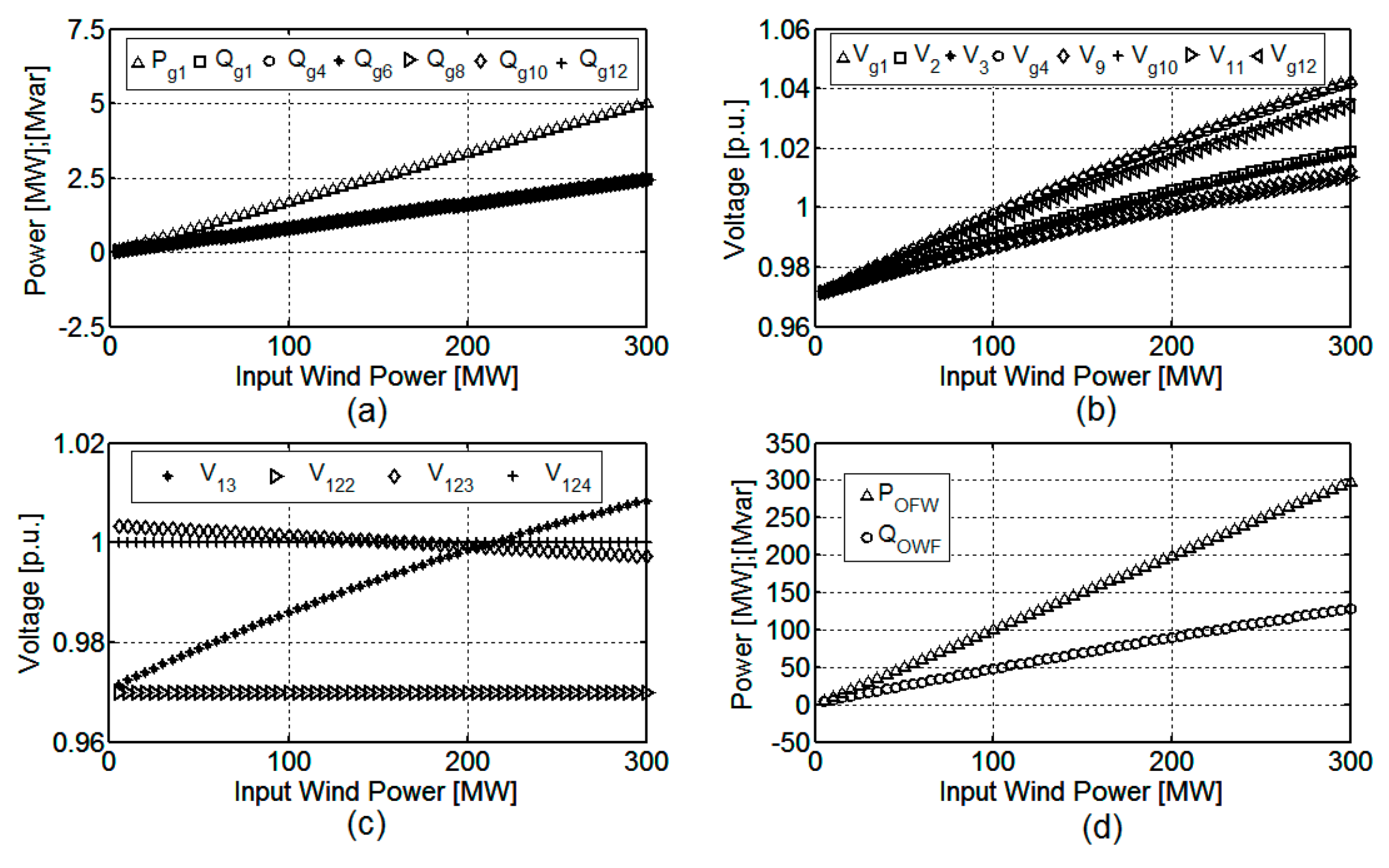
Figure 7.
Steady-state curves without optimization (DFIG pf = 0.9): (a) Active and reactive power at the rectifier side of the VSC-HVdc model; (b) active and reactive at the inverter side of the VSC-HVdc model; (c) DC voltage in the VSC-HVdc model; (d) modulation indexes in the VSC-HVdc model.
Figure 7.
Steady-state curves without optimization (DFIG pf = 0.9): (a) Active and reactive power at the rectifier side of the VSC-HVdc model; (b) active and reactive at the inverter side of the VSC-HVdc model; (c) DC voltage in the VSC-HVdc model; (d) modulation indexes in the VSC-HVdc model.

Figure 8.
Steady-state curves without optimization (DFIG pf = 1.0): (a) Active and reactive power in each DFIG of the first row of the OWF; (b) AC voltage modules of the first row of the OWF; (c) AC voltage module in the VSC-HVdc model; (d) active and reactive power at the bus collection of the OWF.
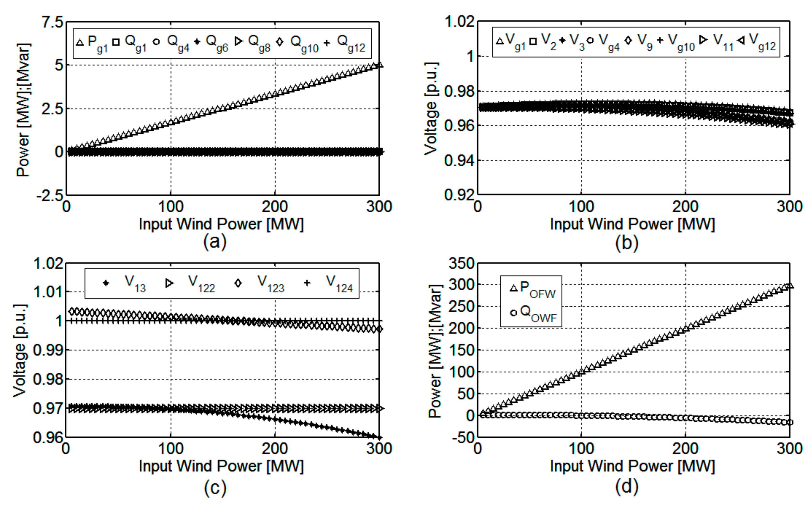
Figure 9.
Steady-state curves without optimization (DFIG pf = 1.0): (a) Active and reactive power at the rectifier side of the VSC-HVdc model; (b) active and reactive at the inverter side of the VSC-HVdc model; (c) DC voltage in the VSC-HVdc model; (d) modulation indexes in the VSC-HVdc model.
Figure 9.
Steady-state curves without optimization (DFIG pf = 1.0): (a) Active and reactive power at the rectifier side of the VSC-HVdc model; (b) active and reactive at the inverter side of the VSC-HVdc model; (c) DC voltage in the VSC-HVdc model; (d) modulation indexes in the VSC-HVdc model.

Figure 10.
Steady-state curves with optimization: (a) Active and reactive power in each DFIG of the first row of the OWF; (b) AC voltage modules of the first row of the OWF; (c) AC voltage module in the VSC-HVdc model; (d) active and reactive power at the bus collection of the OWF.
Figure 10.
Steady-state curves with optimization: (a) Active and reactive power in each DFIG of the first row of the OWF; (b) AC voltage modules of the first row of the OWF; (c) AC voltage module in the VSC-HVdc model; (d) active and reactive power at the bus collection of the OWF.
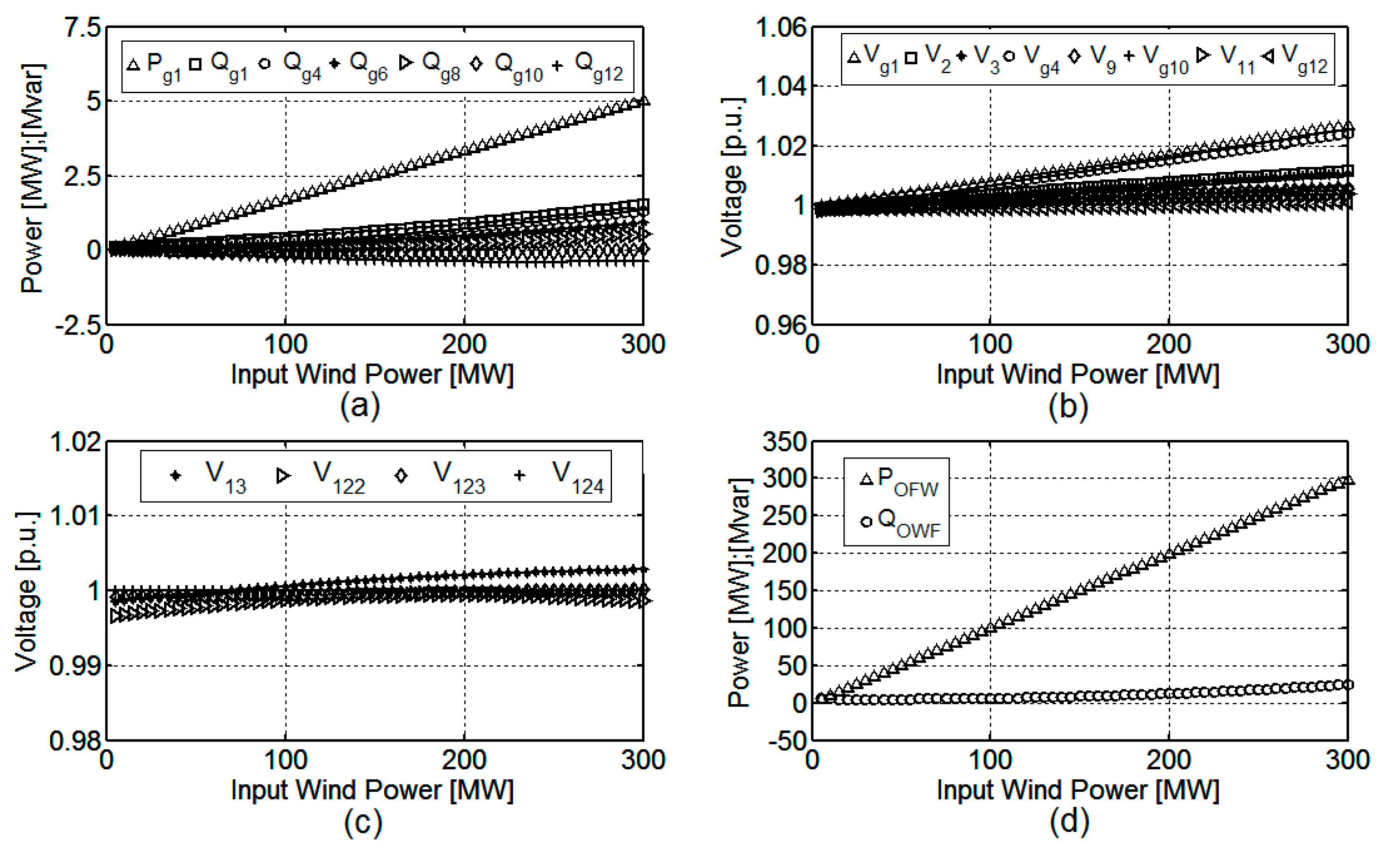
Figure 11.
Steady-state curves with optimization: (a) Active and reactive power at the rectifier side of the VSC-HVdc model; (b) active and reactive power at the inverter side of the VSC-HVdc model; (c) DC voltage in the VSC-HVdc model; (d) modulation indexes in the VSC-HVdc model.
Figure 11.
Steady-state curves with optimization: (a) Active and reactive power at the rectifier side of the VSC-HVdc model; (b) active and reactive power at the inverter side of the VSC-HVdc model; (c) DC voltage in the VSC-HVdc model; (d) modulation indexes in the VSC-HVdc model.

Figure 12.
Power losses: (a) At the OWF; (b) at the OWF+VSC-HVdc.

Table 1.
Line parameters within the offshore wind farm (OWF).
| Z (Ω/km) | C (μF/km) | |
|---|---|---|
| L1 | 0.25 + j0.1351 | 0.17 |
| L2 | 0.25 + j0.1351 | 0.17 |
| L3 | 0.16 + j0.1257 | 0.20 |
| L4 | 0.16 + j0.1162 | 0.23 |
| L5 | 0.10 + j0.1100 | 0.28 |
| L6 | 0.06 + j0.1005 | 0.34 |
Table 2.
AC variables range.
| ac Variable Bus k | Limits | |
|---|---|---|
| Min | Max | |
| Vk (p.u.) | 0.95 | 1.05 |
| φk (°) | −90 | 90 |
| Pk (p.u.) | 0.0 | 1.0 |
| Qk (p.u.) | −1.0 | 1.0 |
| Pgk (p.u.) | 0.0 | 1.0 |
| Qgk (p.u) | −1.0 | 1.0 |
Table 3.
DC-link variables range.
| dc Variables | Limits | |
|---|---|---|
| Min | Max | |
| Pdr,i (p.u.) | 0.0 | 1.0 |
| Qdr,i (p.u.) | −1.0 | 1.0 |
| Udr,i (p.u.) | 0.95 | 1.05 |
| Idc (p.u.) | 0.0 | 1.0 |
© 2017 by the authors. Licensee MDPI, Basel, Switzerland. This article is an open access article distributed under the terms and conditions of the Creative Commons Attribution (CC BY) license (http://creativecommons.org/licenses/by/4.0/).
Share and Cite
MDPI and ACS Style
Montilla-DJesus, M.E.; Arnaltes, S.; Castronuovo, E.D.; Santos-Martin, D. Optimal Power Transmission of Offshore Wind Power Using a VSC-HVdc Interconnection. Energies 2017, 10, 1046. https://doi.org/10.3390/en10071046
AMA Style
Montilla-DJesus ME, Arnaltes S, Castronuovo ED, Santos-Martin D. Optimal Power Transmission of Offshore Wind Power Using a VSC-HVdc Interconnection. Energies. 2017; 10(7):1046. https://doi.org/10.3390/en10071046
Chicago/Turabian StyleMontilla-DJesus, Miguel E., Santiago Arnaltes, Edgardo D. Castronuovo, and David Santos-Martin. 2017. "Optimal Power Transmission of Offshore Wind Power Using a VSC-HVdc Interconnection" Energies 10, no. 7: 1046. https://doi.org/10.3390/en10071046
Note that from the first issue of 2016, this journal uses article numbers instead of page numbers. See further details here.