Performance Predictions of Dry and Wet Vapors Ejectors Over Entire Operational Range

1
College of Environmental Science and Engineering, Taiyuan University of Technology, Taiyuan 030024, China
2
Australasian Joint Research Centre for Building Information Modelling, School of Built Environment, Curtin University, Perth, WA 6845, Australia
*
Author to whom correspondence should be addressed.
Energies 2017, 10(7), 1012; https://doi.org/10.3390/en10071012
Submission received: 12 April 2017
/
Revised: 6 July 2017
/
Accepted: 7 July 2017
/
Published: 17 July 2017
Abstract
:If a traditional ideal-gas ejector model is used to evaluate the performance of a wet vapor ejector, large deviations from the experimental results will be unavoidable. Moreover, the model usually fails to assess the ejector performance at subcritical mode. In this paper, we proposed a novel model to evaluate the performance of both dry and wet vapors ejectors over the entire operational range at critical or subcritical modes. The model was obtained by integrating the linear characteristic equations of ejector with critical and breakdown points models, which were developed based on the assumptions of constant-pressure mixing and constant-pressure disturbing. In the models, the equations of the two-phase speed of sound and the property of real gas were introduced and ejector component efficiencies were optimized to improve the accuracy of evaluation. It was validated that the proposed model for the entire operational range can achieve a better performance than those existing for R134a, R141b and R245fa. The critical and breakdown points models were further used to investigate the effect of operational parameters on the performance of an ejector refrigeration system (ERS). The theoretical results indicated that decreasing the saturated generating temperature when the actual condensing temperature decreases, and/or increasing the saturated evaporating temperature can improve the performance of ERS significantly. Moreover, superheating the primary flow before it enters the ejector can further improve the performance of an ERS using R134a as a working fluid.
1. Introduction
Electrical energy consumed by compressor-based refrigeration systems (CRSs), which provide cooling capacities for air conditioning systems, rapidly grows with people’s increasing demand for thermal comfort [1,2]. Ejector refrigeration technology is an energy-efficient strategy [1,3] and an attractive alternative to a conversional compressor-based refrigeration. Thus, researches on the ejector refrigeration systems (ERSs) have attracted great attentions, in particular theoretical models of ejectors since the ejector is the heart of an ejector refrigeration system.
An ejector refrigeration system (ERS) basically includes an ejector, an evaporator, a generator, a condenser, a pump and an expansion valve, as illustrated in Figure 1. The corresponding thermodynamic cycle is shown in Figure 2. In the generator, the liquid refrigerant is evaporated at high temperature and constant pressure and changed into high saturated vapor (called the primary flow) at point p0, then it enters the ejector and entrains the saturated vapor (called the secondary flow) at point s0, which have provided cooling by evaporating at constant pressure and low temperature in the evaporator. The two streams then mix and the mixed flow experiences a pressure lift in the ejector. At point c, it leaves the ejector as a medium-pressure, superheated vapor, and then enters the condenser to be condensed at constant pressure. At point c1, the liquid refrigerant from the condenser is divided into two parts, one being pumped into the generator at point g, and the other expanding through the expansion valve and entering the evaporator at point e. Then the two parts of refrigerant evaporate in the generator and evaporator, respectively.
Many ideal-gas ejector models for critical mode have been developed as they are simple yet effective in the ejector performance evaluation. Keenan and Newman [4] proposed a 1-D ejector model, which is probably the first constant-area mixing model. Then, Keenan et al. [5] developed a model for a constant-pressure mixing ejector. Munday and Bagster [6] postulated that the secondary flow is choked at a fictive throat and then it mixes with the primary flow under a uniform pressure. Based on Keenan’s model [5], Eames et al. [7] took three isentropic efficiencies to consider losses inside an ejector. Their experimental results were within 85% of theoretical predictions. Huang et al. [8] introduced four ejector component efficiencies to account for losses inside the ejector in their ideal-gas ejector model. Compared with their experiment data of R141b ejectors, the maximum evaluation error is 22.99%. Besagni et al. [9] proposed a model for sonic and sub-sonic ejectors based on the ideal-gas assumption. In the model, the correlation equations of ejector component efficiencies were determined by CFD method. Khennich et al. [10] carried out an exergy analysis of a one-phase ejector taking R141b as the refrigerant and found that large exergy losses are created during the shock. If an ideal-gas model is used to predict the performance of wet-vapor ejectors, large deviations from the experimental results will be unavoidable, since the wet vapor refrigerants, such as R11, R22, and etc., usually deviate far from the ideal gas law [11]. To address this issue, real gas treatment was introduced in ejector models for critical mode. Lear et al. [12] presented a 1-D ejector model, which can handle the two-phase flow in an ejector with Fabri choking. Cardemil and Colle [13] proposed a real-gas ejector model. The evaluation results show good agreement with the experimental data for the R141b [8], water [14] and carbon dioxide [15] ejectors operating at critical modes.
All the ejector models mentioned above are only capable of evaluating the ejector performance at critical mode. To date, a few attempts were made to develop the ejector model for the entire operational range, including critical and subcritical modes. Chen et al. [16] extended the ideal-gas ejector model of Huang et al. [8] to the entire operational range. The prediction errors at subcritical mode were about 20%. Chen et al. [11] also proposed a real-gas ejector model for the entire operational range. For the dry vapor refrigerant R141b, the prediction errors of critical condensing pressure and entrainment ratio were within ±9% and ±17%, respectively. For the wet vapor refrigerant R11, the maximum error of COP was −31.58%.
From the literature review above, it is found that there are few ejector models, which can predict the ejector performance over the entire operational range with high accuracy, especially for wet vapors ejectors. The main objective of this paper is hence to propose a novel model for both dry and wet vapor ejectors over the entire operational range. To obtain high accuracy, the following strategies were adopted: (1) developing the critical and breakdown points models based on constant-pressure mixing and constant-pressure disturbing, and integrating them with linear characteristic equations of ejector to form the model; (2) introducing real gas property and the equations of sound speed with high evaluation accuracy into the models; (3) adopting the analysis method of the effect of change (EOC) of the efficiencies [17] and the sparsity-enhanced optimization method [18] to identify and determine the correlation equations of ejector components efficiencies. Then, the model was employed to analyze the influences on the ejector performance induced by superheating the primary flow before it enters the ejector.
2. Preliminaries
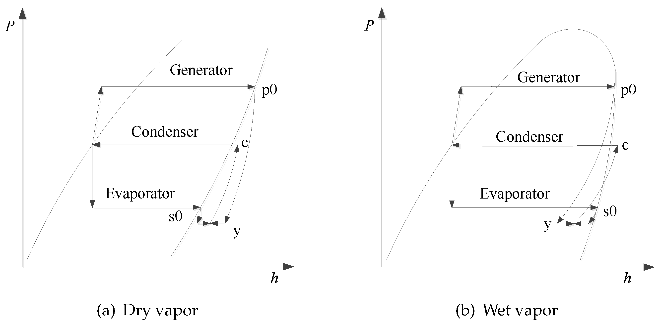
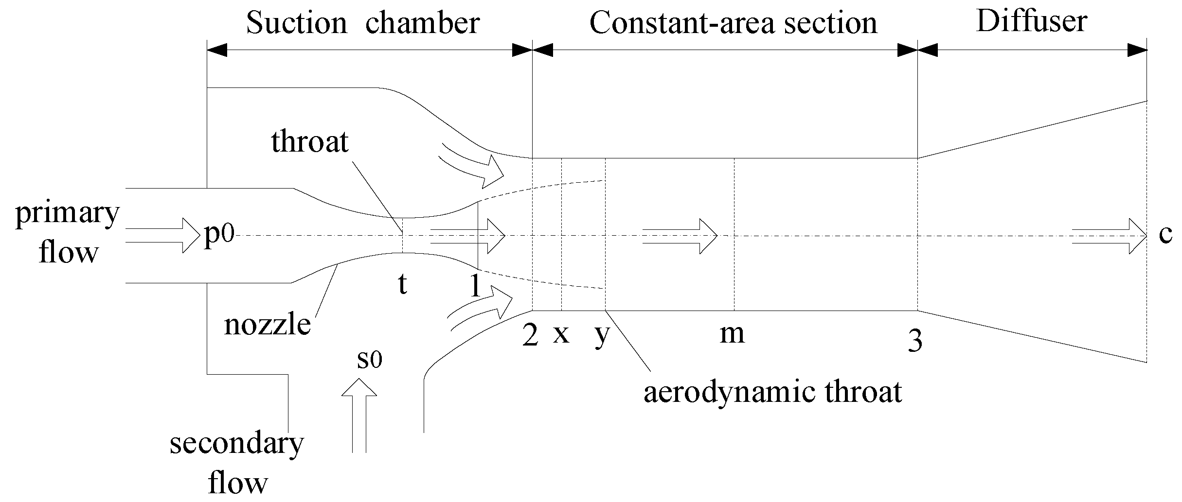
Ejector is a compression component of an ERS and the entrainment ratio u, which is the ratio between the mass flow rate of the secondary flow and the primary flow, is a key parameter of it. Schematic diagram of an ejector is shown in Figure 3. The working fluids of ERSs are classified into two categories: wet vapor (R11, R12, R134a or Steam) and dry vapor (R113, R123 or R141b) [19]. The thermodynamic cycle for the two working fluids are shown in Figure 2. It can be observed that during the expansion of the primary flow in the nozzle, the isentropic line for wet working fluid goes into the wet vapor region. While for dry working fluid, it goes into the superheated region. It can be deduced that the property of wet vapor is far from that of ideal gas.
2.1. Operation Modes
Figure 4 illustrates the three operational modes of ejector. The modes are divided by the two key points, i.e., critical point, at which entrainment ratio u equals critical entrainment ratio and condensing pressure equals critical condensing pressure , and breakdown point, at which and is equal to breakdown condensing pressure . The three operational modes are:
- Critical mode: the primary flow and the secondary flow are choked at the nozzle throat and section y-y, respectively, and u is constant, as ;
- Subcritical mode: only the primary flow is choked at the nozzle throat and u decreases with as ;
- Back-flow mode: no choking phenomenon exists and as .
For critical mode, the performance characteristic equation of ejector and its boundary are:
For subcritical mode, the performance characteristic equation of ejector and its boundary are:
2.2. Assumptions
It can be found that the ejector loses its function at backflow mode as indicated in Figure 4. Thus, the entire operational range only includes the critical and subcritical modes. The prediction performance at critical mode can be obtained by , , Equations (1) and (2). Similarly, the model at subcritical mode can be obtained by , , , Equations (3) and (4). Therefore, the ejector model over the entire operational range can be developed based on the models at the critical and breakdown points. To develop the ejector models at the critical and breakdown points, we require the following assumptions:
- The inner wall of the ejector is adiabatic and the flow is one dimensional and steady inside the ejector;
- The kinetic energy of the primary flow at the nozzle inlet, the secondary flow at the suction inlet and the mixing flow at the diffuser outlet are negligible;
- Constant-pressure mixing exists at critical point. After fanning out of the nozzle, the primary flow entrains but does not mix with the secondary flow before section y-y. The secondary flow is choked at section y-y and starts to mix with the primary flow with a uniform pressure, i.e., before the shock;
- Constant-pressure disturbing occurs at breakdown point. The primary and secondary flows do not mix before section x-x. Then, before the shock, the secondary flow disturbs the the primary flow by mixing in and out of the primary flow with a uniform pressure, i.e., .
3. Ejector Performance Modelling
3.1. Model for the Critical Point
3.1.1. Primary Flow from Inlet to Nozzle Throat
According to assumption (2), the inlet enthalpy is thought as stagnant enthalpy. Then the energy conservation equation is:
where and are enthalpy and velocity at nozzle throat, respectively. The velocity equals the sound of speed since the primary flow is choked at throat, namely
where, is the speed of sound at the nozzle throat. For single phase state, it can be obtained directly from NIST [20]; for wet vapor, the calculation method of it will be described in Section 3.3. In general, it can be expressed as the following relation:
where,
In this model, the isentropic efficiency is introduced to account for the losses during the expansion process, and it should be determined by experimental data. It is defined as:
where is the enthalpy obtained after a hypothetical isentropic expansion from the inlet to the nozzle throat. It can be expressed as:
where is the entropy of the primary flow corresponding to the hypothetical enthalpy at throat, which equals the entropy at the inlet of nozzle. is the pressure at throat, which is a parameter used to determine the speed of sound and can be derived by an iterative process using Equations (5)–(10).
The primary flow rate is obtained by the following relation:
3.1.2. Primary Flow from Throat to Exit of Nozzle
The energy conservation equation during this process is:
where and are enthalpy and velocity at nozzle exit, respectively.
The velocity meets the following mass conservation equation:
where,
This process is a simple expansion process since the back pressure, namely, the pressure of the secondary flow are much less than that of the primary flow in nozzle throat and thus oblique shocks will occur out of the nozzle [13] rather than between the throat and the exit of nozzle. Thus, it is assumed that the expansion process is approximately isentropic as other ejector models. Then, the entropy of the primary flow at the exit of nozzle, , follows:
Then,
3.1.3. Primary Flow from Nozzle Exit to Section y-y
The energy conservation equation between the nozzle exit and section y-y is:
where and are enthalpy and velocity at section y-y, respectively.
The velocity meets the following mass conservation equation:
where,
The isentropic efficiency is used to considering the losses cause by the oblique shocks during the expansion process, and it is defined as:
where is the enthalpy of the secondary at section y-y after an isentropic expansion process, it follows:
where, , according to the assumption (3).
3.1.4. Secondary Flow from Suction Inlet to Section y-y
According to the assumption (2), the suction enthalpy of the secondary flow is treated as the stagnant enthalpy. Then, the energy conservation equation is:
where, is velocity of the secondary flow at section y-y, and it equals the speed of sound according to the assumption (3), i.e.,
where, is the speed of sound of the secondary flow at section y-y. It can be expressed as:
where,
During the expansion process, the isentropic efficiency is defined as
where is the enthalpy of the secondary flow at section y-y after an isentropic expansion from suction to section y-y. It follows:
where is the entropy corresponding to the enthalpy at section y-y and it equals ; is the pressure at section y-y, which is a parameter used to determine the speed of sound. It can be obtained by an iterative process using Equations (22)–(27).
The secondary flow rate is derived by the following relation:
The area follows:
3.1.5. Mixing and Shock in Constant Section
The mixing starts at section y-y with a uniform pressure . The energy conservation equation can be expressed as:
Since the mixing occurs under constant pressure in the mixing chamber whose sectional-area are constant, the momentum conservation equation can be expressed as :
where is the momentum transfer efficiency which is used to account for the losses during the mixing of the two streams. The density of the mixed flow is:
The pressure rises from to when the mixed flow passes through the shock wave. They meet the following equation [13]:
The energy conservation equation can be expressed as:
Hugoniot equation [21] expresses the thermodynamic parameter relationship while the flow experiences a normal shock wave:
where,
3.1.6. Diffuser
The energy conservation equation of the mixed flow exhausting from diffuser is expressed as follows:
where is the enthalpy at the exit of diffuser when the ejector operates at critical point. Introducing to express the efficiency during the compression process. Then
where is the enthalpy obtained by an ideal isentropic compression process, i.e.,
During the hypothetic isentropic process, the pressure recovers from to . The critical condensing pressure , i.e., the pressure at the exit of the diffuser after a real process, is equal to , namely,
3.2. Model for the Breakdown Point
3.2.1. Primary Flow from Inlet to Nozzle Exit
3.2.2. Primary Flow from Nozzle Exit to Section x-x
The process is approximately an isentropic process, i.e.,
According to the assumption (4), at section x-x, the pressure of the primary flow equals that of the secondary flow. i.e. . Then,
The velocity of the primary flow at section x-x, , can be obtained by the following energy conservation equation:
3.2.3. Secondary flow at section x-x
According to the assumption (4), the secondary flow does not mix with the primary flow before section x-x. Thus, the energy of the secondary flow at section x-x equals , i.e.,
At breakdown point, the entrainment ratio equals zero, then it can be assumed that the velocity of the secondary flow is small enough and the pressure of the secondary flow at section x-x equals inlet pressure, i.e., .
3.2.4. Constant Pressure Disturbing
Although the entrainment ratio is equal to zero, the breakdown condensing pressure, , is changed with the pressure of the secondary flow. Obviously, the secondary flow has an effect on , in other words, the secondary flow disturbs the primary flow to influence as assumption (4). To consider this effect, it is assumed that the flow rate of the secondary flow is small enough and equals kg/s and introducing the momentum transfer efficiency in momentum conservation equation to account for the losses from section x-x to section m-m.
Applying the energy conservation, gives:
The momentum conservation equation is:
According assumption (4), the constant-pressure disturbing starts at section x-x with a uniform pressure, that is . Then, the density of the flow is:
3.2.5. Diffuser
Assuming the kinetic energy being zero at exit of diffuser, the energy conservation equation is expressed as:
where is the enthalpy at the exit of diffuser at breakdown point. The isentropic efficiency is defined as:
where is the enthalpy after an ideal isentropic compression process, i.e.,
The pressure at the exit of the diffuser in a real process is equal to , which is corresponding to the enthalpy . Then
3.3. Speed of Sound of Wet Vapor
For wet-vapor working fluid, the flow in the nozzle throat is in two-phase state. Although droplets formed in the throat are so less, they obviously affect the speed of sound of the flow and the ejector performance. Khaled Ameur et al. [22] proposed relations to calculate two-phase speed of sound. They also conducted comparisons with several available methods on two-phase speed of sound and found that Wood’s equation [23] provided relatively good predictions. Tao et al. [24] also found that Wood’s equation agrees well with experimental data [25]. Here the Wood’s equation is introduced in our models which is
where and are the speed of sound of saturated liquid and vapor, respectively, is the void fraction of vapor; and are the densities of saturated liquid and vapor, respectively; is the density of two-phase vapor, it is:
It is assumed that: (1) the gas phase medium and the liquid phase medium are uniformly mixed together; (2) it is an adiabatic process; (3) there is no surface tension and the pressure of liquid phase is equal to that of vapor phase. Then the wood’s equation can be deduced as follows:
The bulk modulus of elasticity of the fluid K is the ratio between stress and strain :
The stress and strain meet the following relationship in the two-phase vapor:
The bulk modulus of elasticity follows:
3.4. Model over Entire Operational Range
As discussed above, the critical point model and breakdown point model are basic models for the model over the entire operational range. We developed the critical point model by modifying the model of Cardemil and Colle [13]. Moreover, we proposed a novel breakdown point model for both dry and wet vapor based on the constant-disturbing assumption. Then, the critical and breakdown points models can be integrated with linear characteristic Equations (1) and (3) and the boundaries Equations (2) and (4) to form the novel model for the entire operational range.
4. Experimental Verification
To obtain more accurate prediction performance, the ejector component efficiencies should be determined carefully since they dramatically influence the validity of an ejector model [26] and the values of the efficiencies depend on the ejector geometry, working fluid and operation conditions [8,9]. In this paper, five efficiencies, , , , and are introduced in critical point model. is used to consider the losses during the mixing of the primary and secondary flows, and , , , are the isentropic efficiencies of the primary flow from inlet to the throat of the nozzle and from the exit of the nozzle to section y-y of the ejector, the efficiency of the secondary flow from suction to hypothetical throat, and the efficiency of the mixed flow in diffuser, respectively. Even though they have physical meaning, they act as a correct factors in generally cases [27]. Thus, they should be determined based on experimental data.
We will employ the experiment data for R134a [28], R141b [8] and R245fa [1] ejectors to determine the efficiencies and verify our models. The physical parameters, safety and environmental data of these refrigerants are listed in Table 1. R141b is viewed as a higher efficiency refrigerant for an ERS, but it will be phased out due to its ozone depletion potential (ODP). R134a was widely used in the refrigeration systems as an alternative environment friendly refrigerant from point of ODP, toxicity and flammability. Although the US Environmental Protection Agency (EPA) announced the timetable for eliminating the use of it and it will be limited to use according to the EU Regulation 517/2014 due to its high global warming potential (GWP), it can be used in other countries. R245fa is a dry refrigerant, its properties in ODP and GWP are similar with those of R134a, but its applications are less than R134a as its safety class is in B1.
A program was developed to calculate the ejector performance over the entire operational range. The flowchart is shown in Figure 5, where the sub-flowcharts for calculating the speed of sound and the parameters of shock wave are shown in Figure 6. The properties of refrigerants are calculated by REFPROP Version 9.0 [20]. EOC analysis method proposed in [17] was employed to analyze the influence of the efficiencies. From [17], larger absolute value of average EOC indicates that the efficiency has larger influence on the prediction accuracy of . The same applies to EOC and the prediction accuracy of . Based on the experimental data of R134a ejectors in [28], the absolute values of average EOC for , , , and are 2.0, 1.11, 0.13, 0, 0, respectively; and those of average EOC for , , , and are 0.48, 0.20, 0.12, 0.86, 0.11, respectively. It can be found that, in terms of prediction , the efficiencies and have more influence than the other efficiencies, and, for , the efficiencies and have more impact than the other efficiencies. For R141b, the effects of the efficiencies are similar with those for R134a. Hence, the efficiencies and are taken as constant since entrainment ratio and critical condensing pressure are not sensitive to them. The other efficiencies were determined by sparsity-enhanced optimization [18] based on the foregoing experiment. For the ejector model at breakdown point, three component efficiencies are used, and are taken as those in the critical point model due to the same choking phenomenon and compression process, respectively, and will be expressed as correlation equations as breakdown condensing pressure is sensitive to it.
4.1. R134a Ejector
R134a is a typical wet-vapor refrigerant. The experimental data [28] are taken to validate the ejector model using R134a as a working fluid. An experimental ejector consists of two parts: the nozzle and the ejector body, which includes suction chamber, constant-area section and diffuser. Thus, nozzles and ejector bodies can interchange. The throat and exit diameters are 2.5 and 3.3 mm for nozzle A, and 2.09 and 2.7 mm for nozzle B, respectively. The diameters of mixing chambers A and B are 4.16 and 3.81 mm, respectively. The efficiency is taken as 0.88 as that in [8] and is adopted as 0.95 as that in [13]. Based on 20 cases of experimental data at critical points, the other efficiencies are derived through sparsity-enhanced optimization:
These correlations of efficiencies should be used within the following boundaries:
The comparisons between the theoretical prediction results and the experiment data are shown in Table 2. It can be seen that the theoretical results of critical condensing pressures coincide fairly well with the measured , most of the errors are within ± 3% and the maximum prediction error is 3.71%. For critical entrainment ratios , most of them are within ± 6% deviation in comparison with the measured and the maximum error is 6.97%. The estimated speed of sound of the primary flow at nozzle throat, , is also reported in Table 2. It can be observed that mainly relates to the saturated temperature and varies slightly with and . This is because that the speed of sound relates to , and as indicate in Equation (5) to (10), and the efficiency varies with and as indicated in Equation (58).
For the breakdown point, the choking of the primary flow is the same as that at critical point. Thus, the ejector component efficiency is taken as that at critical point, namely, . Based on 12 cases at breakdown points, the optimized result of and its boundaries are:
The theoretical values of breakdown condensing pressure versus experimental data for breakdown points are shown in Figure 7. It can be observed that the theoretical values of breakdown condensing pressure are within ±2% deviation from the experimental data.
For the entire operational range, the theoretical and experimental performances in terms of condensing pressures are illustrated in Figure 8. It is obviously that the theoretical coincide fairly well with the experimental values, and deviations are within ±12% over the entire operational range.
4.2. R141b Ejector
In the experiment of Huang et al. [8], they tested the performance of 11 ejectors at critical points. The area ratios of ejectors range from 6.44 to 10.64, the pressures of the primary flow and the secondary flow vary from 0.400 MPa to 0.604 Mpa and from 0.040 MPa to 0.047 MPa, respectively.
As we have mentioned before, the efficiencies and are taken as 0.88 and 0.95, respectively. The other efficiencies are optimized based on the experimental data and the methods in [18]. They are:
These correlations of efficiencies should be used within the following boundaries:
The theoretical results of ejector performance are compared with the experimental data as shown in Table 3. As can be seen, most of theoretical results of critical condensing pressure are within ±4% deviation in comparison with the measured values and the maximum error is 6.73%. For critical entrainment ratio , the maximum error is 7.70%. The estimated speed of sound of the primary flow at nozzle throat, , is summarized in Table 3. It can be seen that relates to , and although the variations of for R141b are less than those for R134a.
4.3. R245fa Ejector
The experimental results of Shestopalov et al. [1] were used to validate our model over the entire operational range. In the experiment, R245fa was used as a working fluid, and 9 ejectors for 11 critical-point cases and 1 ejector for 3 cases over the entire operational range were tested, respectively.
As those for R141b, the efficiencies and are adopted as 0.88 and 0.95 in critical point model, respectively. The other efficiencies were obtained through optimizing them to fit the experiment data. They are:
The boundaries for these correlations of efficiencies are:
The model validation for critical condensing pressure and are illustrated in Figure 9a,b, respectively. As shown in the figures, both and are agree fairly well with the experimental results. More specifically, the prediction errors of and are within ±2% and ±5%, respectively.
For the breakdown point model, the efficiencies and are taken as those in critical point model. The efficiency was derived by fitting the calculated breakdown condensing pressures to the experimental values in [1]. The obtained optimum correlation and its boundaries are:
For the entire operational range, the experimental and calculated entrainment ratios u in terms of condensing temperatures are plotted in Figure 10. It can be observed that the prediction values coincide with experimental results very well. Further observation finds that the prediction accuracy of breakdown condensing temperatures at breakdown point is higher than that of critical entrainment ratios and critical condensing temperatures . In fact, the prediction errors of are within ±0.5%.
5. Results and Discussion
For wet vapor refrigerant, droplets will form in the nozzle when the primary flow expands through the nozzle. However, for dry vapor refrigerant, the vapor is in superheated state in the nozzle. Droplets in nozzle will affect ejector performance. In this paper, wet vapor refrigerant R134a and dry vapor refrigerants R141b and R245fa are selected to perform the comparison. A R134a ejector and a R141b ejector were designed to meet the same design conditions at critical point; more specifically, cooling capacity = 1.5 kW, saturated generating temperature °C, saturated evaporating temperature = 10 °C and critical condensing temperature °C. The key geometric parameters of the R134a ejector are: = 2.491 mm, = 3.177 mm, = 4.96 mm. For the R141b ejector, = 4.261 mm, = 7.80 mm, = 10.865 mm. To simplify the analysis, it is assumed that the losses from the generator and the evaporator to the ejector are ignored, and the inlet pressures and are corresponding to saturated temperatures and , respectively.
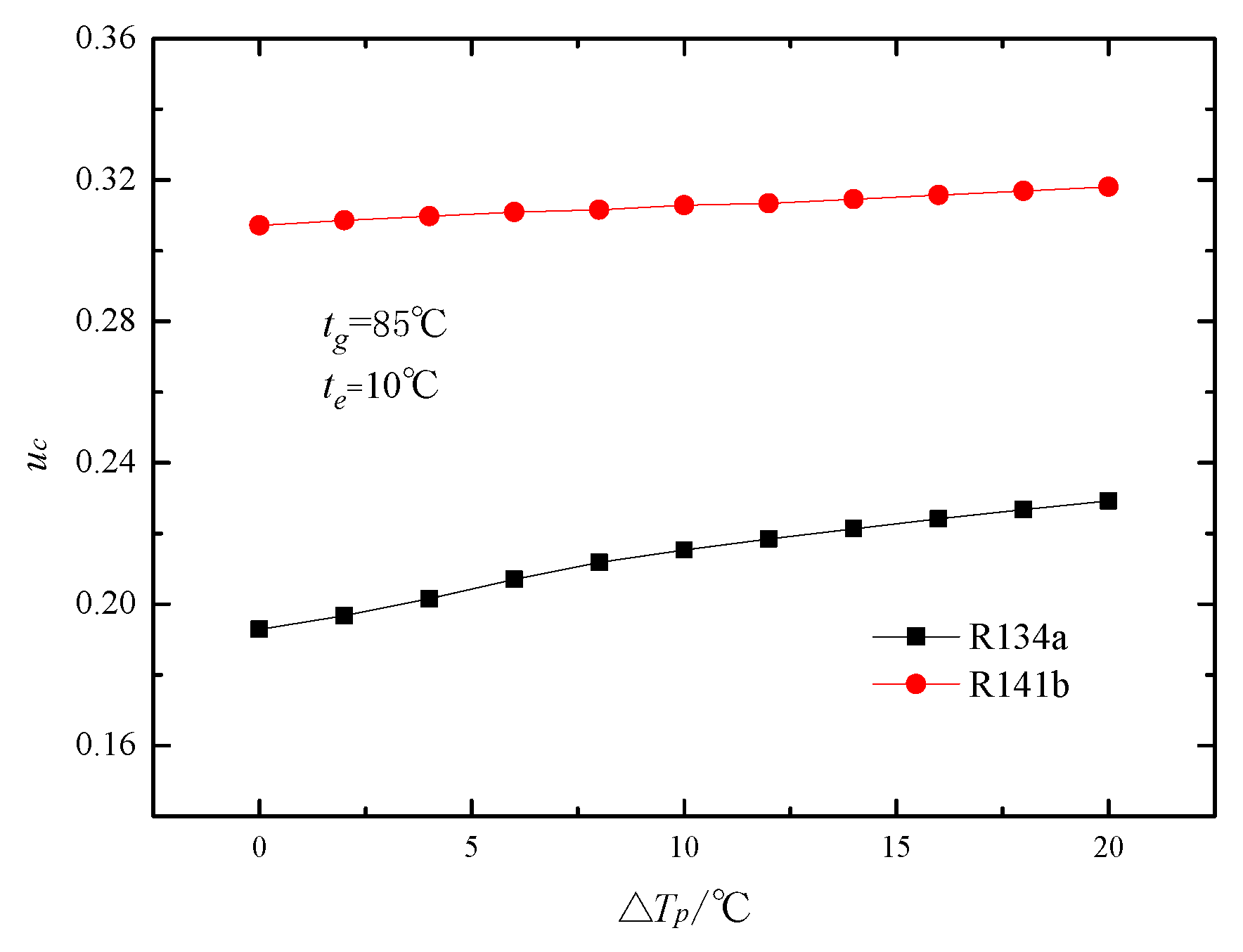
Figure 11 shows the critical entrainment ratio versus the superheating degree △ of the primary flow. It can be observed that for the R134a ejector, is lower than that for the R141b ejector. For the R141b ejector, increases slightly and uniformly with the increasing of △, but for the R134a ejector, increases more rapidly at low △ than at high △, with the inflection point being at about △ 8 °C. Since , the increasing of may be induced by the increasing of and/or the decreasing of .
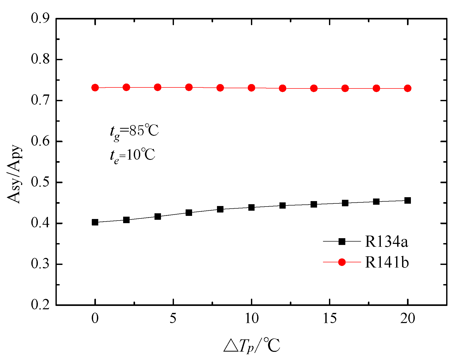
The flow rates and vs. △ are plotted in Figure 12a,b, respectively, and vs. △ is shown in Figure 13. As can be seen, the increasing rate of , the decreasing rate of and increasing rate of of the R134a ejector are all lessened after △ grows higher than 8 °C. The inflection point of these curves are all at △ °C. According to the calculation results of the vapor quality, R134a is in wet vapor state at section y-y as △ °C; after that, it changes into superheated vapor. Thus, the inflection of the variations rate of , , and the resultant change of are induced by the phase change of the primary flow at section y-y.
For the R141b ejector, the variation rates of , , and are less than those for the R134a ejector, and there is no significant change in the variation rate as shown in Figure 11 to Figure 13. The main reason is that R141b stays at the superheated-vapor state rather than the wet vapor state as △ is changed. Thus, superheating R134a before it enters the ejector has much higher influence than superheating R141b.
Figure 14 shows the cooling capacity over the primary superheating △. It can be found that has the same variation trend as since the enthalpies at the inlet and the outlet of the evaporator have no variation. Superheating the primary flow is helpful in increasing for a R134a ejector ( increased by 10% at △ = 20 °C). However, for a R141b ejector, shows no change.
The coefficient of performance (COP) is often employed in evaluating the performance of a refrigeration system. For an ERS, it is defined as the ratio of cooling capacity to energy input which includes generating heat and pump power . Generally, since is much less than , it has less influence on COP. Figure 15 depicts COP over the superheating temperature △. For R134a, COP has no significant variation with △, although increases with the increasing of △ as shown in Figure 14. This is because superheating the primary flow will cost more energy. In other words, the increasing rate of is close to that of . For R141b, COP decreases with rise in △. This lies in that superheating the primary flow costs more energy, whereas, the cooling capacity is almost constant.
Figure 16 illustrates the critical condensing temperature v.s. the primary superheating △. It can be seen that for the R134a ejector, has a slight increase when △ increases, but for the R141b ejector, remains almost constant. The difference may be mainly induced by the different variation of , which equals to the speed of sound at the nozzle. The calculation results indicate that increases by 14% and 4% for the R134a ejector and the R141b ejector, respectively, when △ changes from 0 to 20 °C. Thus, the increment of for the R134a ejector is larger than that for the R141b ejector. When △ varies from 0 to 20 °C, the increments of the outlet temperature of the ejector are about 26 °C and 17 °C for the R134a ejector and R141b ejector, respectively. It should be noticed that the above is not the outlet temperature of the diffuser but the saturated temperature which is corresponding to the critical condensing pressure .
Besagni et al. [26] studied the optimum ejector performance, which is obtained by adjusting area ratio to a suitable value in relation to the variations of generating, evaporating and condensing temperature. This is significant for the design of an ERS. However, for operating an ERS, it seems more helpful to find the coupled influence of operating conditions and superheating on the performance of the ejector at fixed .
Figure 17 illustrates the variations of ejector performance with saturated generating temperature using R134a as a working fluid. It can been seen that, for the same , the critical entrainment ratio at °C is larger than that at °C, but COPs are almost the same at both °C and °C. As those have indicated in Figure 11 and Figure 14, except the rise in , superheating the primary flow can also cause the rise in cooling capacity . In terms of critical condensing temperature , superheating the primary flow can increase it slightly when > 85 °C as shown in Figure 17b. Thus, for wet-vapor R134a, it can be concluded that superheating the primary flow has insignificant influence on COP, but can increase the cooling capacity . In fact, further observation on Figure 17 finds that the effect of the change of is much more significant than that of superheating the primary flow. Namely, COP and both increase sharply with the decrease of . Therefore, for a given ERS, decreasing the saturated generating temperature can result in significant increase in both and COP when the actual condensing temperature is lower than .
Figure 18 depicts the ejector performance v.s. the saturated generating temperature using R141b as a working fluid. It can be observed that when °C, the critical entrainment ratio has a diminutive rise and COP has a slight decrease relative to those at °C, but has hardly any variation when the primary flow is superheated at °C. Referring to Figure 11 and Figure 14, it can be deduced that can not increase for each in the range from 70 to 95 °C. Thus, for an ERS using dry-vapor refrigerant R141b, superheating primary flow could not improve its performance.
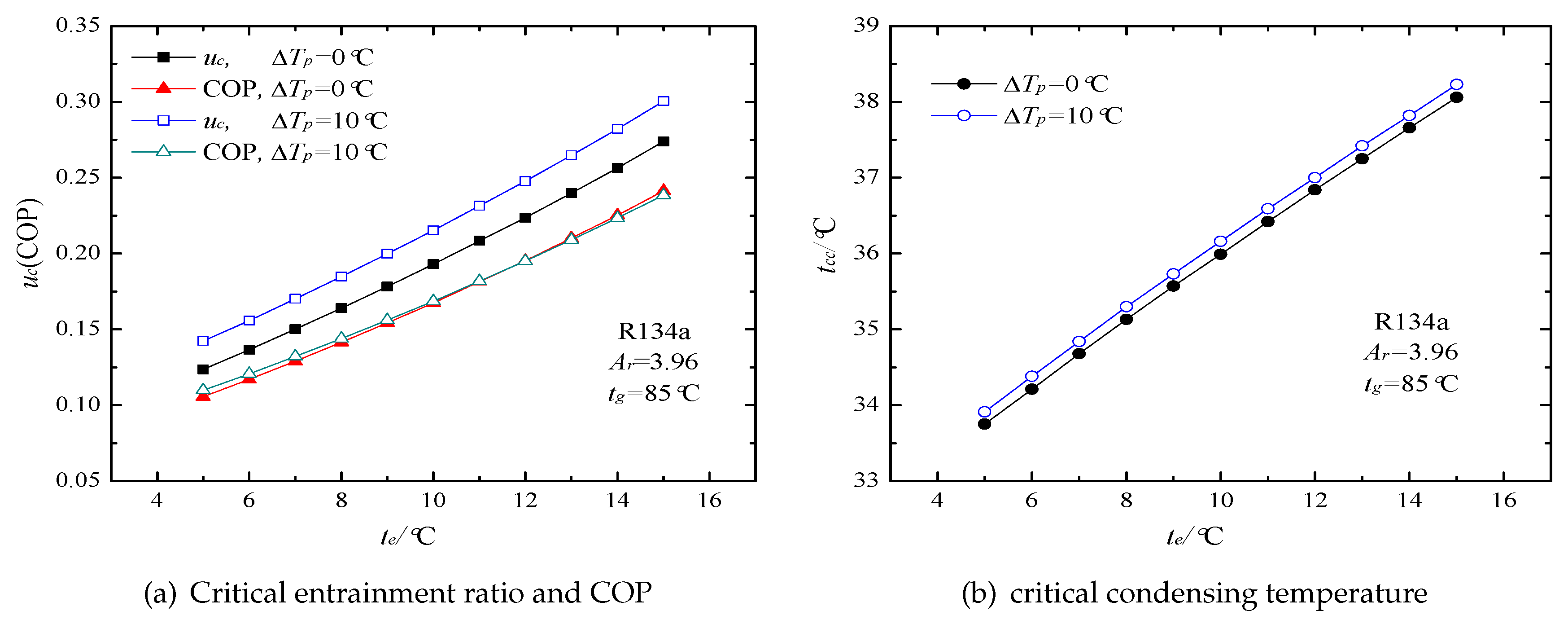
Figure 19 shows the ejector performance v.s. the saturated evaporating temperature using R134a as a working fluid. For each , the critical entrainment ratio and critical condensing temperature at °C are both larger than those at °C, but COP are almost the same for the two conditions. Referring to Figure 11 and Figure 14, it can be deduced that can be larger at = 10 °C than that °C for each . Thus, for saturated generating temperature = 85 °C, superheating primary flow can lead to some increase in and of an ERS using R134a as a working fluid. However, COP, u and all rapidly increase with rise in . This means increasing of has more significant influence on the performance of an ERS than superheating the primary flow. However, it is certain that for each , superheating the primary flow can further improve the cooling capacity .
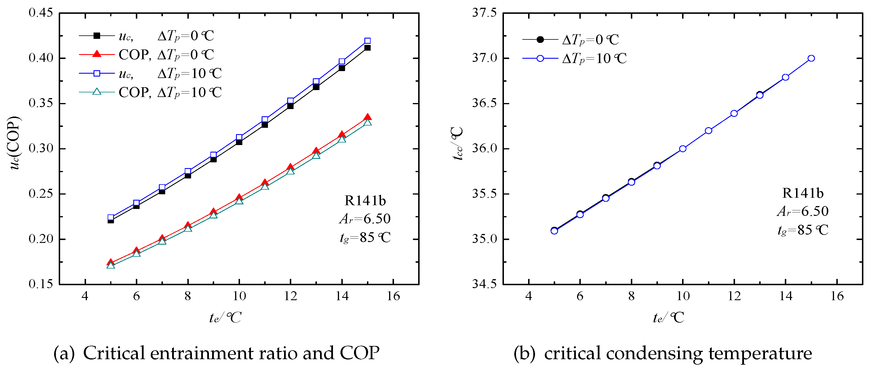
Figure 20 illustrates the ejector performance v.s. the evaporating temperature using R141b as a working fluid. It is found that for the ejector with fixed , the critical entrainment ration at °C is a little larger than that at °C and COP is slightly lower than that at °C for each . As shown in Figure 20b, has hardly any variation when changes from 0 to 10 °C. Thus, superheating the primary flow has little influence on the performance of an ERS using R141b as a working fluid. However, it can be observed that the performance, namely u, COP and , of an ERS can be obviously improved with a rise in .
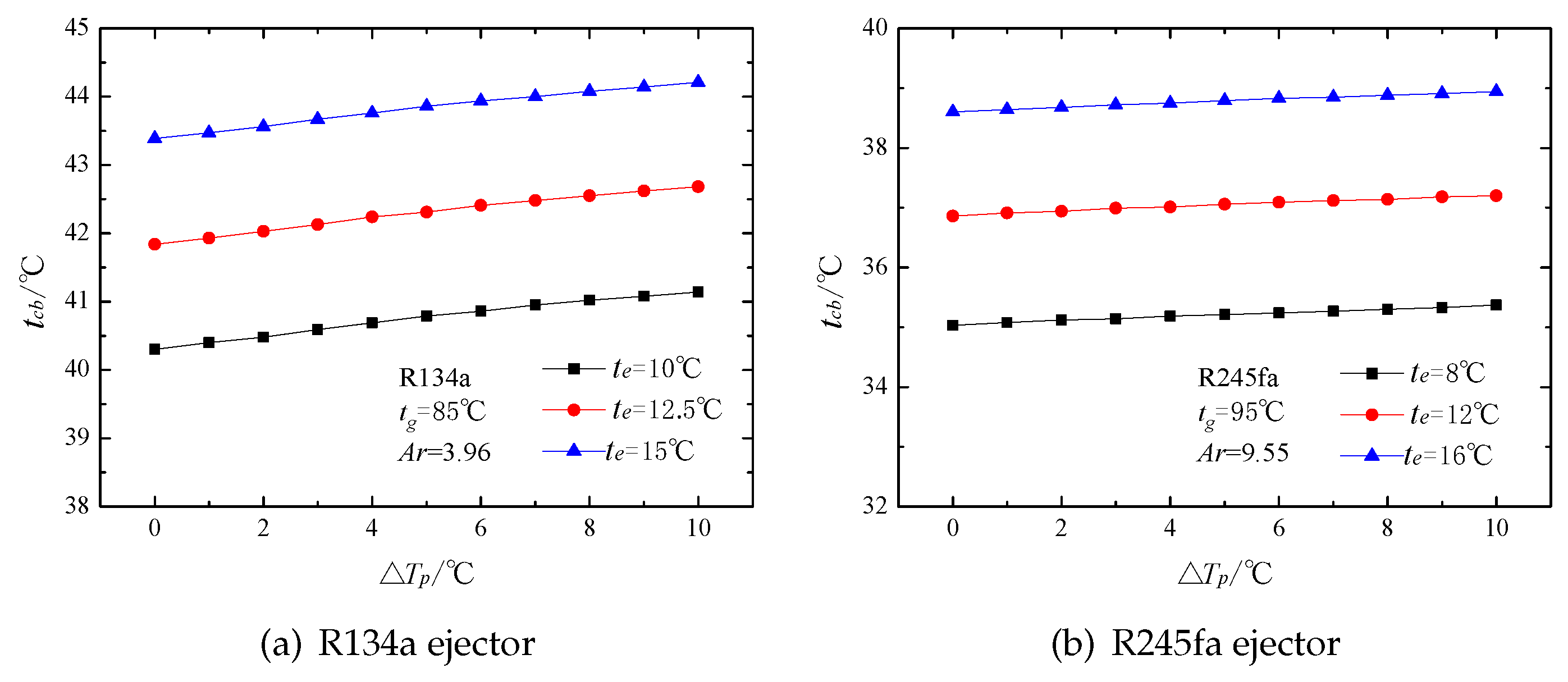
For the breakdown point model, R134a and R245fa are used as working fluids to analyze the ejector performance vs. the primary superheating △. Figure 21a,b show the breakdown condensing temperature in terms of the primary superheating △ for a R134a ejector and a R245fa ejector, respectively. is corresponding to the breakdown condensing pressure . It can be observed that increases with the rise in △. For the R134a ejector, has up to 2% rise at △ = 10 °C, but for a R245fa ejector, the increasing of is insignificant. This is mainly because the variation rate of sound speed in the nozzle throat is different for the two ejectors. It is known that the speed of sound sharply increases as the working fluid changes from wet vapor to dry saturated vapor. Hence, the increasing rate of the sound speed in the nozzle throat of the R134a ejector, is larger than that of the R245fa ejector since R134a changes from two-phase state to vapor state as △ rises from 0 to 10 °C, but for R245fa, it maintains at superheating vapor state. Further observations indicate that the increasing rate is similar for different . This indicates that has no significant influence on the variation rate of when △ is changed.
6. Conclusions
This paper proposed a novel model for the performance predictions of dry and wet vapor ejectors over the entire operational range. The model was obtained by integrating the linear characteristic equations of ejector with critical and breakdown points models, which were developed based on the assumptions of constant-pressure mixing and constant-pressure disturbing. To improve the accuracy of the models, equations of the real gas property and the two-phase speed of sound were introduced and the ejector component efficiencies were determined through EOC analysis and sparsity-enhanced optimization. The theoretical results of the model coincided fairly well with the experimental data for both dry and wet refrigerants over the entire operational range.
It was also found that superheating the primary flow before it enters the ejector can improve the ejector performance. For the R134a ejector, when the primary superheating △ changed from 0 to 20 °C, the critical entrainment ratio and cooling capacity could be increased by 19% and 10%, respectively. For the R141b ejector with the same design conditions as the R134a ejector, increased insignificantly with the enlarging △. For the breakdown point, the condensing temperature had some rise when △ increased. For both wet and dry working fluids, critical entrainment ratios , coefficients of performance COP and critical condensing temperatures could be improved significantly with rising in saturated evaporating temperature . However, for a given ERS, decreasing the saturated generating temperature can result in significant increase in both and COP when the actual condensing temperature decreases. If the primary flow is superheated together with the increase of or the decrease of , and can be further improved for wet working fluid R134a.
Acknowledgments
This research is supported by the Natural Science Foundation of China (50976074, 61473326), Key Science and Technology Program of Shanxi Province, China (20140313006-6), Research Project Supported by Shanxi Scholarship Council of China (2016-032).
Author Contributions
Fenglei Li and Qi Tian designed the study. Fenglei Li and Zhao Chang performed the simulations. Fenglei Li wrote the first draft of the paper. Changzhi Wu and Xiangyu Wang reviewed the manuscript.
Conflicts of Interest
The authors declare no conflict of interest.
Abbreviations
The following abbreviations are used in this manuscript:
| COP | the coefficient of performance |
| CRS | compressor-based refrigeration system |
| EOC | the effect of the change (of efficiency) |
| ERS | ejector refrigeration system |
Nomenclature
| a | speed of sound (m/s) |
| A | area (m) |
| d | diameter (m) |
| h | enthalpy (kJ/kg) |
| K | bulk modulus of elasticity (N/m) |
| m | mass flow rate (kg/s) |
| P | pressure (MPa) |
| s | entropy (kJ/kg K) |
| t | temperature (°C) |
| T | temperature (K) |
| u | entrainment ratio |
| v | velocity (m/s) |
| void fraction of vapor | |
| strain | |
| efficiency relating to isentropic efficiency | |
| density (kg/m) | |
| stress (N/m) | |
| efficiency account for losses | |
| infinitesimal | |
| Subscripts | |
| b | breakdown |
| c | condensation, critical point |
| d | diffuser |
| e | expansion, evaporation |
| g | generation |
| l | liquid |
| m | mixing flow |
| p | primary flow |
| primary flow at inlet of ejector | |
| primary flow at nozzle exit | |
| r | ratio |
| s | secondary flow, isentropic process |
| secondary flow at inlet of ejector | |
| t | throat |
| v | vapor |
| y | position of the hypothetical throat |
References
- Shestopalov, K.; Huang, B.; Petrenko, V.; Volovyk, O. Investigation of an experimental ejector refrigeration machine operating with refrigerant R245fa at design and off-design working conditions. Part 1. Theoretical analysis. Int. J. Refrig. 2015, 55, 201–211. [Google Scholar] [CrossRef]
- Umair, M.; Akisawa, A.; Ueda, Y. Performance evaluation of a solar adsorption refrigeration system with a wing type compound parabolic concentrator. Energies 2014, 7, 1448–1466. [Google Scholar] [CrossRef]
- Akiloroaya, V.; Samali, B.; Fakhar, A.; Pishghadam, K. A review of different strategies for HVAC energy saving. Energy Convers. Manag. 2014, 77, 738–754. [Google Scholar] [CrossRef]
- Keenan, J.H.; Neumann, E.P. A simple air ejector. ASME J. Appl. Mech. 1942, 9, A75–A81. [Google Scholar]
- Keenan, J.H. An investigation of ejector design by analysis and experiment. J. Appl. Mech. 1950, 17, 299–309. [Google Scholar]
- Munday, J.T.; Bagster, D.F. A new ejector theory applied to steam jet refrigeration. Ind. Eng. Chem. Process. Des. Dev. 1977, 16, 442–449. [Google Scholar] [CrossRef]
- Eames, I.W.; Aphornratana, S.; Sun, D.W. The jet-pump cycle: A low cost refrigerator option powered by waste heat. Heat Recover. Syst. CHP 1995, 15, 711–721. [Google Scholar] [CrossRef]
- Huang, B.J.; Chang, J.M.; Wang, C.P.; Petrenko, V.A. A 1-D analysis of ejector performance. Int. J. Refrig. 1999, 22, 354–364. [Google Scholar] [CrossRef]
- Besagni, G.; Mereu, R.; Chiesa, P.; Inzoli, F. An integrated lumped parameter-CFD approach for off-design ejector performance evaluation. Energy Convers. Manag. 2015, 105, 697–715. [Google Scholar] [CrossRef]
- Khennich, M.; Sorin, M.; Galanis, N. Exergy flows inside a one phase ejector for refrigeration Systems. Energies 2016, 9, 212. [Google Scholar] [CrossRef]
- Chen, W.; Shi, C.; Zhang, S.; Chen, H.; Chong, D.; Yan, J. Theoretical analysis of ejector refrigeration system performance under overall modes. Appl. Energy 2017, 185, 2074–2084. [Google Scholar] [CrossRef]
- Lear, W.E.; Parker, G.M.; Sherif, S.A. Analysis of two-phase ejectors with Fabri choking. Arch. Proc. Inst. Mech. Eng. C-J. Mech. 2002, 216, 607–621. [Google Scholar] [CrossRef]
- Cardemil Cardemil, J.M.; Colle, S. A general model for evaluation of vapor ejectors performance for application in refrigeration. Energy Convers. Manag. 2012, 64, 79–86. [Google Scholar] [CrossRef]
- Chen, Y.M.; Sun, C.Y. Experimental study of the performance characteristics of a steam-ejector refrigeration system. Energy Convers. Manag. 1997, 15, 384–394. [Google Scholar] [CrossRef]
- Xu, X.; Chen, G.; Tang, L.; Zhu, Z.; Liu, S. Experimental evaluation of the effect of an internal heat exchanger on a transcritical CO2 ejector system. J. Zhejiang Univ.-Sci. A 2011, 12, 146–153. [Google Scholar] [CrossRef]
- Chen, W.; Liu, M.; Chong, D.; Yan, J.; Little, A.B.; Bartosiewicz, Y. A 1D model to predict ejector performance at critical and sub-critical operational regimes. Appl. Therm. Eng. 2013, 36, 1750–1761. [Google Scholar] [CrossRef]
- Li, F.; Tian, Q.; Wu, C.; Wang, X.; Lee, J.M. Ejector performance prediction at critical and subcritical operational modes. Appl. Therm. Eng. 2017, 115, 444–454. [Google Scholar] [CrossRef]
- Li, F.; Wu, C.; Wang, X.; Tian, Q.; Teo, K.L. Sparsity-enhanced optimization for ejector performance prediction. Energy 2016, 113, 25–34. [Google Scholar] [CrossRef]
- Chen, S.L.; Yen, J.Y.; Huang, M.C. Experimental investigation of ejector performance based upon different refrigerants. ASHRAE Trans. 1998, 104, 153–160. [Google Scholar]
- Lemmon, E.; Huber, M.; McLinden, M. NIST Standard Reference Database 23: Reference Fluid Thermodynamic and Transport Properties-REFPROP, version 9.1; National Institute of Standards and Technology: Gaithersburg, MD, USA, 2010. [Google Scholar]
- Anderson, J. Modern Compressible Flow, 2nd ed.; McGraw-Hill: New York, NY, USA, 2002. [Google Scholar]
- Ameur, K.; Aidoun, Z.; Ouzzane, M. Modeling and numerical approach for the design and operation of two-phase ejectors. Appl. Therm. Eng. 2016, 109, 809–818. [Google Scholar] [CrossRef]
- Wood, A.B. A Textbook of Sound, 3rd ed.; Neill and Co. Ltd: London, UK, 1957. [Google Scholar]
- Tao, B.; Chen, D.H.; Che, C.X.; Wang, X.M. Study on the sound velocity in a gas-liquid flow. J. Appl. Acoust. 2015, 34, 373–376. [Google Scholar]
- Henry, R.E.; Grolmes, M.A.; Fauske, H.K. Pressure-Pulse Propagation in Two-Phase One- and Two-Component Mixtures; ANL: Chicago, IL, USA, 1971. [Google Scholar]
- Besagni, G.; Mereu, R.; Leo, G.D.; Inzoli, F. A study of working fluids for heat driven ejector refrigeration using lumped parameter models. Int. J. Refrig. 2015, 58, 154–171. [Google Scholar] [CrossRef] [Green Version]
- Varga, S.; Oliveira, A.C.; Diaconu, B. Numerical assessment of steam ejector efficiencies using CFD. Int. J. Refrig. 2009, 32, 1203–1211. [Google Scholar] [CrossRef]
- Li, F. Study on Ejectors and a Solar Ejector-Refrigeration System with Dual Energy-Storage Tanks and Mulitiple Ejectors. Ph.D. Thesis, Taiyuan Univesity Technology, Taiyuan, China, 2016. [Google Scholar]
Figure 1.
Equipments diagram for basic ejector refrigeration system.
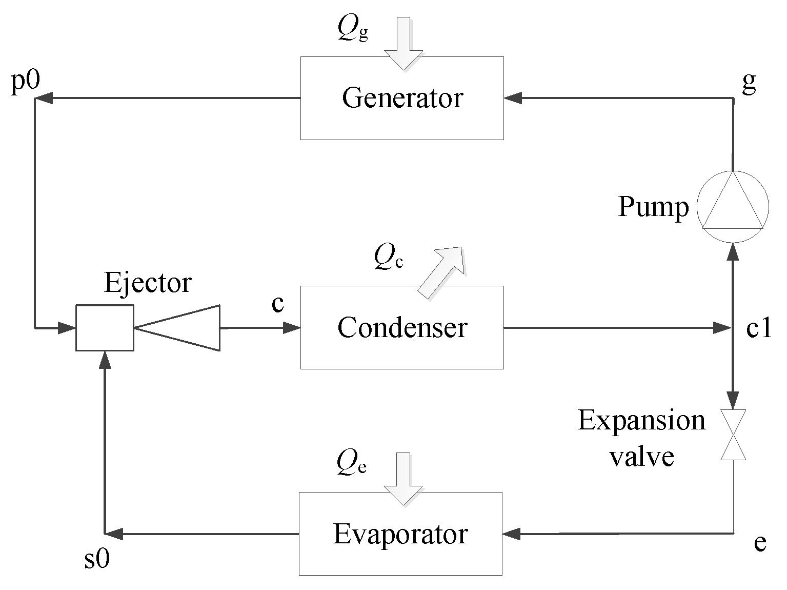
Figure 2.
Pressure-enthalpy charts for ejector refrigeration cycles with dry and wet vapors.

Figure 3.
Schematic diagram of ejector.

Figure 4.
Operational modes of ejector.
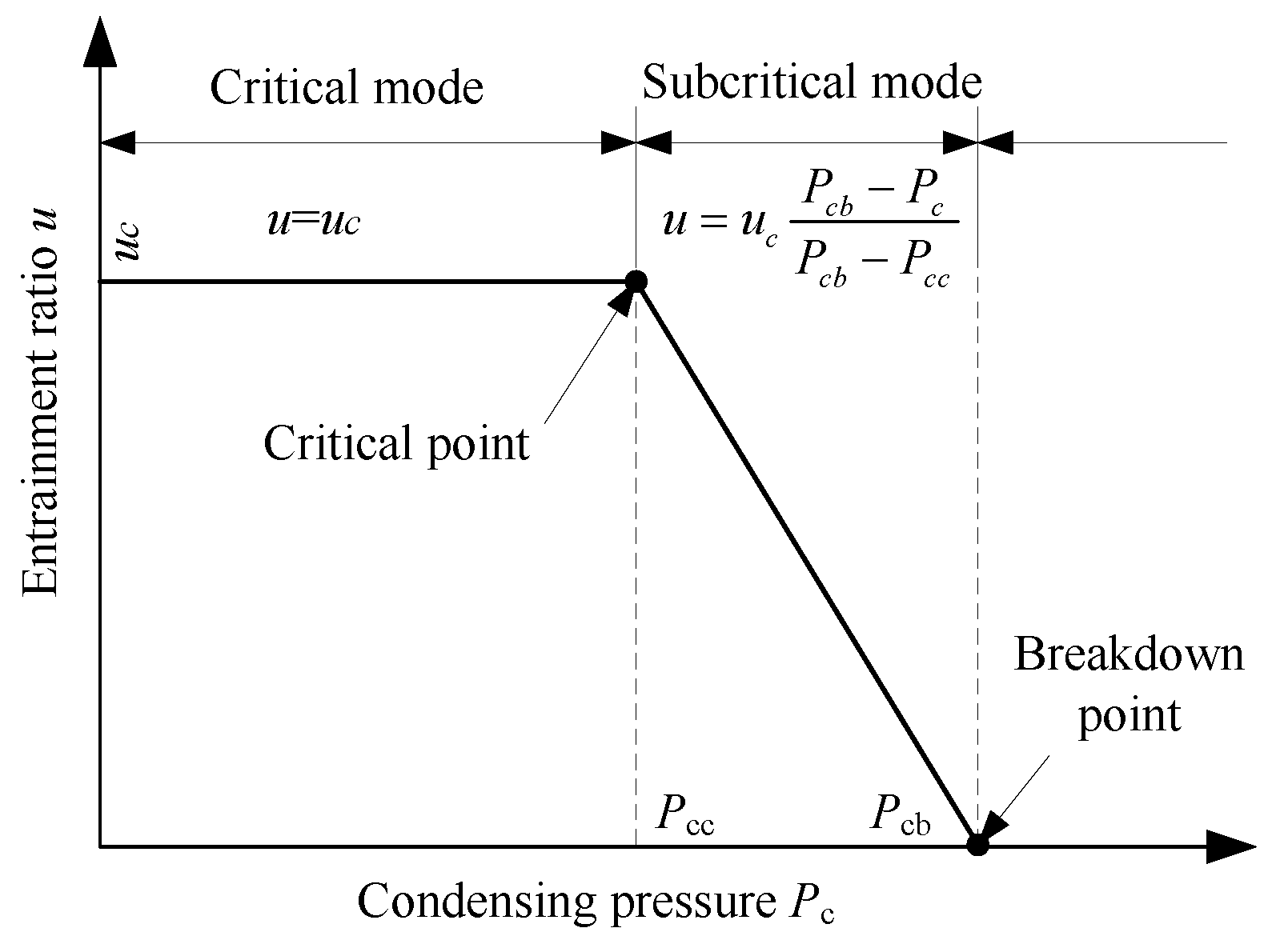
Figure 5.
The flowchart of calculation.

Figure 6.
Sub-flowchart for calculation of the speed of sound and the parameters of shock wave.
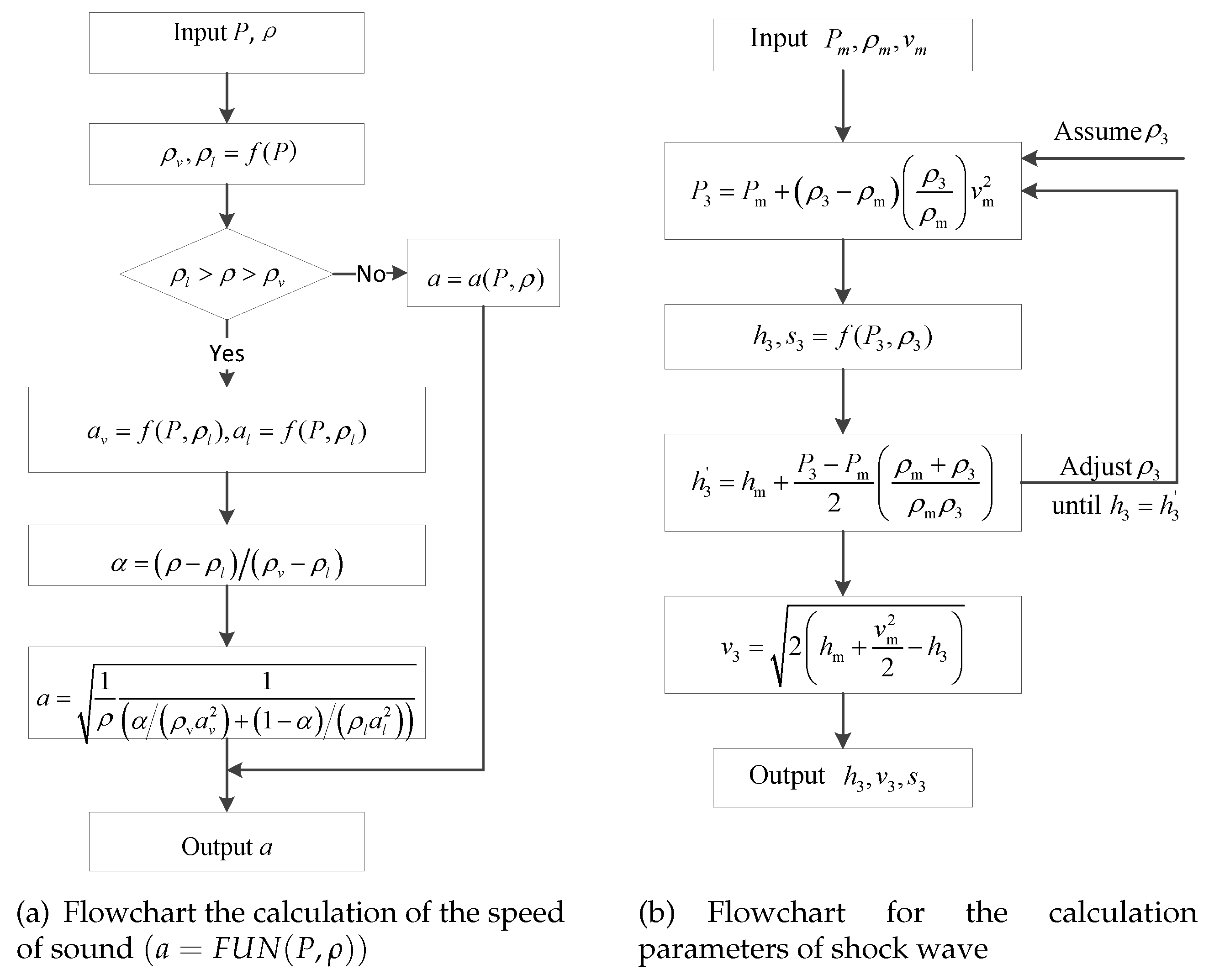
Figure 7.
Comparisons of theoretical breakdown condensing pressures with experimental values using R134a as a working fluid.
Figure 7.
Comparisons of theoretical breakdown condensing pressures with experimental values using R134a as a working fluid.

Figure 8.
Comparisons of theoretical entrainment ratios with experimental values using R134a as a working fluid.
Figure 8.
Comparisons of theoretical entrainment ratios with experimental values using R134a as a working fluid.

Figure 9.
Comparisons of theoretical values of critical condensing pressure and critical entrainment ratios with experimental data using R245fa as a working fluid.
Figure 9.
Comparisons of theoretical values of critical condensing pressure and critical entrainment ratios with experimental data using R245fa as a working fluid.

Figure 10.
Comparisons of theoretical entrainment ratios with experimental values using R245fa as a working fluid.
Figure 10.
Comparisons of theoretical entrainment ratios with experimental values using R245fa as a working fluid.
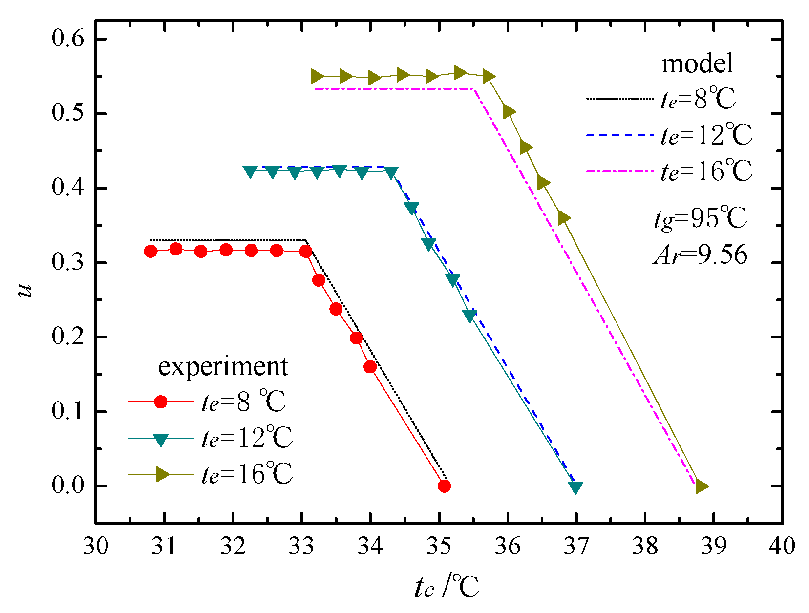
Figure 11.
Entrainment ratio versus the primary superheating △.

Figure 12.
The flow rates of the primary and secondary flows versus the primary superheating △.
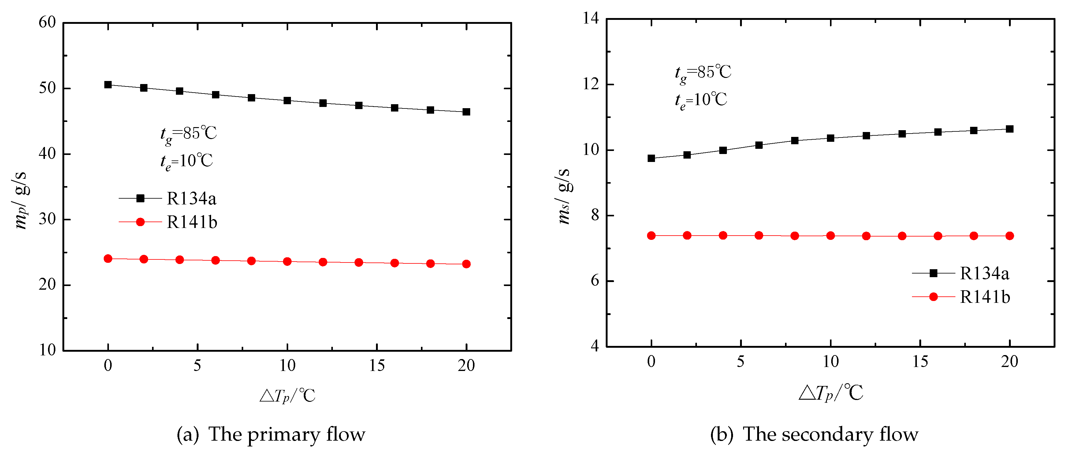
Figure 13.
Area ratio versus the primary superheating △.

Figure 14.
Cooling capacity versus the primary superheating △.
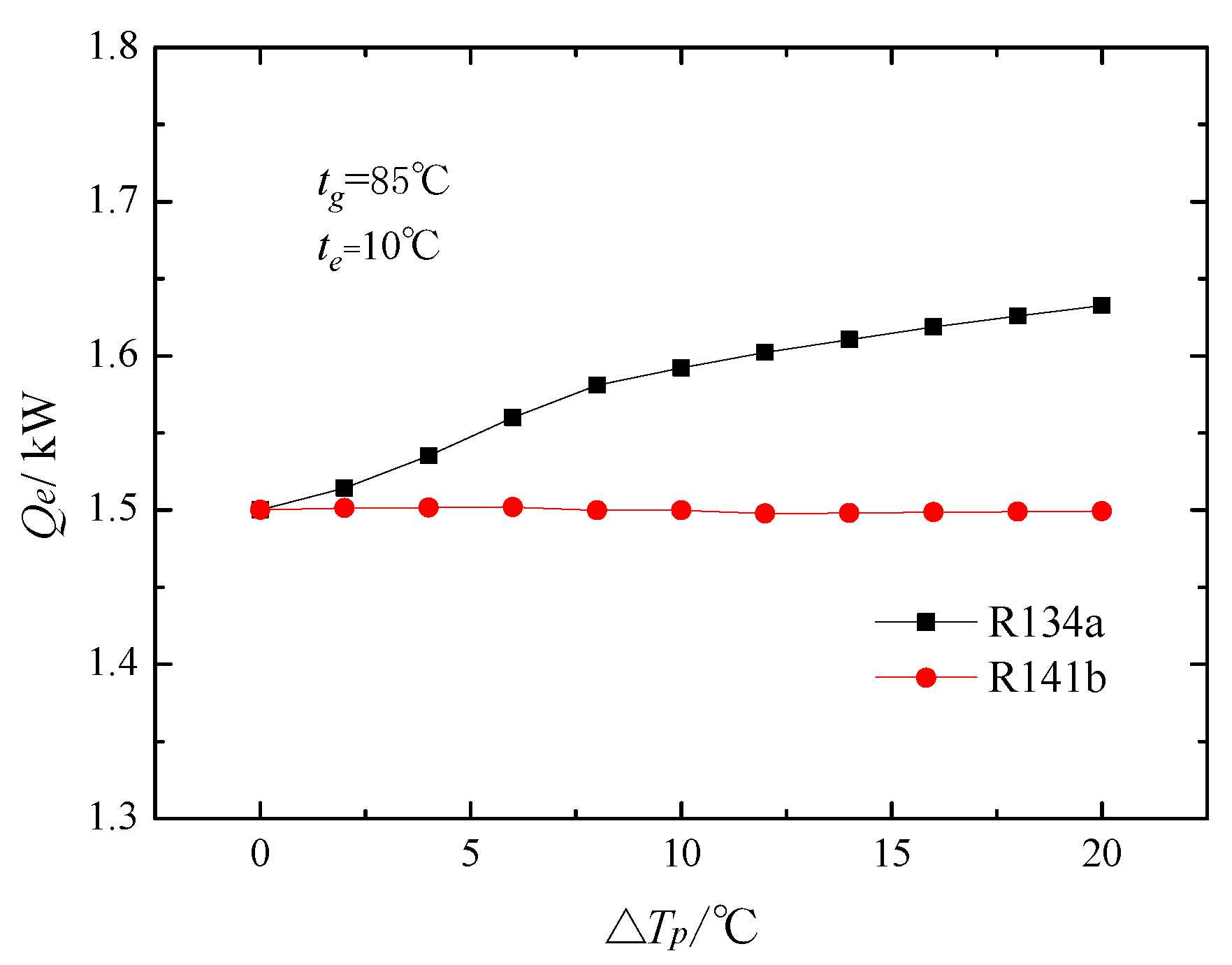
Figure 15.
The coefficient of performance COP versus the primary superheating △.
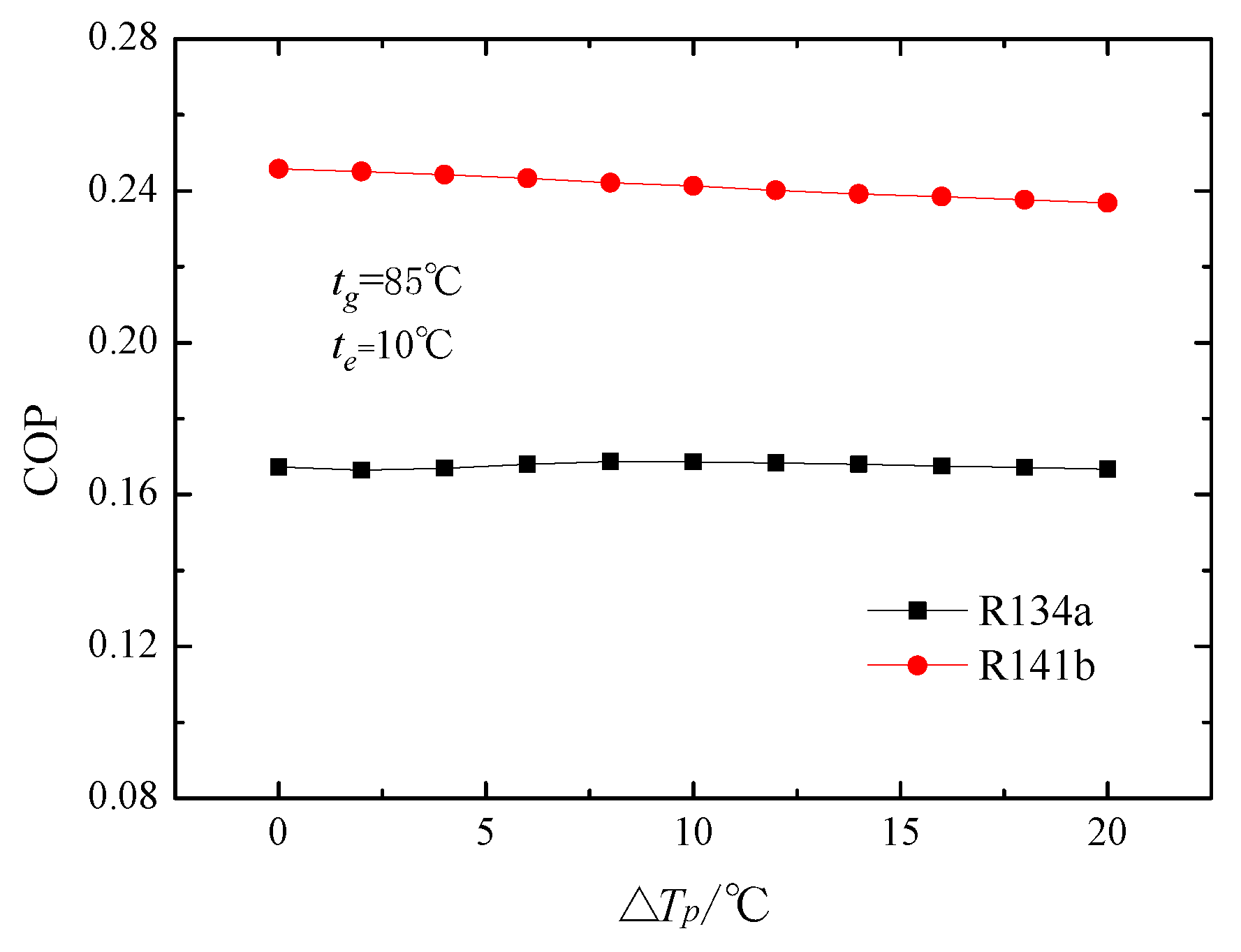
Figure 16.
Critical condensing temperature versus the primary superheating △.
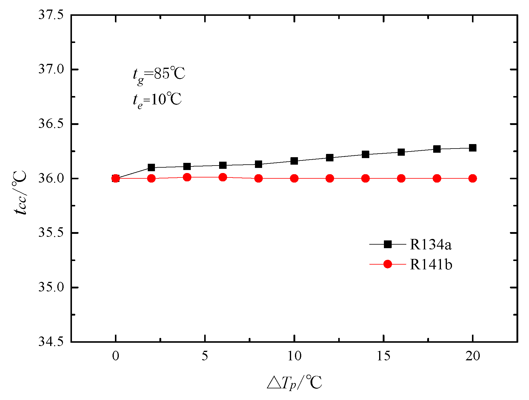
Figure 17.
Critical entrainment ratio, COP and critical condensing temperature versus generating temperature using R134a as a working fluid.
Figure 17.
Critical entrainment ratio, COP and critical condensing temperature versus generating temperature using R134a as a working fluid.
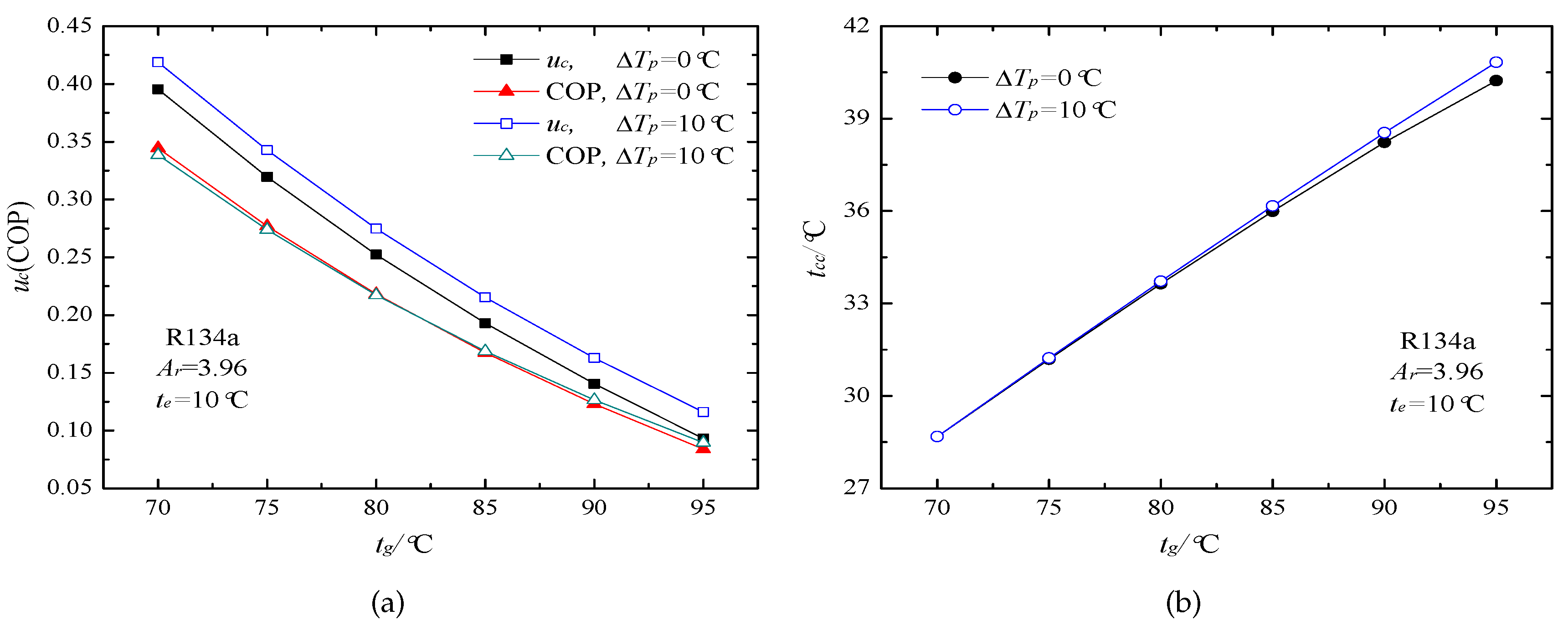
Figure 18.
Critical entrainment ratio, COP and critical condensing temperature versus generating temperature using R141b as a working fluid.
Figure 18.
Critical entrainment ratio, COP and critical condensing temperature versus generating temperature using R141b as a working fluid.
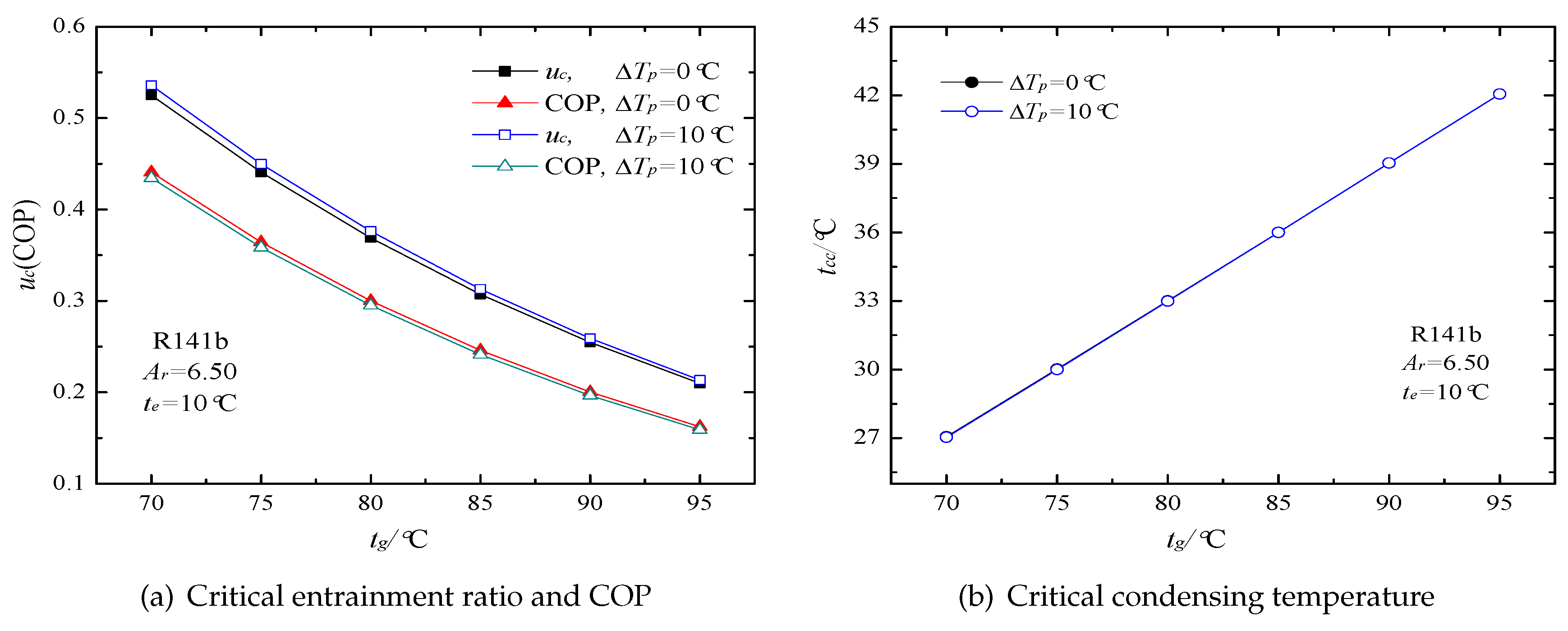
Figure 19.
Critical entrainment ratio, COP and critical condensing temperature versus evaporating temperature using R134a as a working fluid.
Figure 19.
Critical entrainment ratio, COP and critical condensing temperature versus evaporating temperature using R134a as a working fluid.

Figure 20.
Critical entrainment ratio, COP and critical condensing temperature versus evaporating temperature using R141b as a working fluid.
Figure 20.
Critical entrainment ratio, COP and critical condensing temperature versus evaporating temperature using R141b as a working fluid.

Figure 21.
Breakdown condensing temperature versus the primary superheating △ for R134a and R245fa ejectors.
Figure 21.
Breakdown condensing temperature versus the primary superheating △ for R134a and R245fa ejectors.


Table 1.
Thermophysical prosperities, safety and environmental data of the tested working fluid.
| Refrigerant | Molecular Mass | Boiling Point | Critical Temperature | Critical Pressure | Safety Group | ODP | GWP |
|---|---|---|---|---|---|---|---|
| (°C) | (°C) | (MPa) | |||||
| R134a | 102.03 | −26.1 | 101.1 | 4.06 | A1 | 0 | 1370 |
| R141b | 116.95 | 32.0 | 204.4 | 4.21 | A2 | 0.12 | 717 |
| R245fa | 134.05 | 15.1 | 154.0 | 3.65 | B1 | 0 | 1050 |
Table 2.
Comparisons between critical point model and the experiment results for R134a ejectors.
| A | Theory | Experiment | Errors | Theory | Experiment | Errors | |||
|---|---|---|---|---|---|---|---|---|---|
| (°C) | (°C) | (MPa) | (MPa) | (%) | (%) | (m/s) | |||
| AA Ejector | |||||||||
| 2.77 | 75 | 10 | 0.8969 | 0.885 | 1.35 | 0.0844 | 0.0836 | 1.01 | 137.2 |
| 2.77 | 75 | 12.5 | 0.9203 | 0.8974 | 2.55 | 0.1149 | 0.1224 | −6.14 | 137.0 |
| 2.77 | 75 | 15 | 0.9426 | 0.9351 | 0.80 | 0.1472 | 0.1561 | −5.72 | 136.7 |
| BB Ejector | |||||||||
| 3.32 | 75 | 10 | 0.8461 | 0.8553 | −1.08 | 0.1929 | 0.1933 | −0.19 | 136.9 |
| 3.32 | 75 | 12.5 | 0.8685 | 0.8655 | 0.35 | 0.2325 | 0.2209 | 5.24 | 136.7 |
| 3.32 | 75 | 15 | 0.8906 | 0.8808 | 1.11 | 0.2749 | 0.257 | 6.97 | 136.5 |
| 3.32 | 80 | 10 | 0.9071 | 0.9278 | −2.23 | 0.1402 | 0.1411 | −0.65 | 134.8 |
| 3.32 | 80 | 12.5 | 0.9324 | 0.9354 | −0.32 | 0.1749 | 0.1757 | −0.45 | 134.5 |
| 3.32 | 80 | 15 | 0.9568 | 0.9598 | −0.31 | 0.2118 | 0.2055 | 3.08 | 134.2 |
| 3.32 | 85 | 12.5 | 0.9964 | 1.0049 | −0.85 | 0.1235 | 0.1172 | 5.35 | 131.9 |
| 3.32 | 85 | 15 | 1.024 | 1.035 | −1.06 | 0.1562 | 0.1532 | 1.97 | 131.6 |
| BA Ejector | |||||||||
| 3.96 | 75 | 10 | 0.7984 | 0.7994 | −0.12 | 0.3195 | 0.3248 | −1.64 | 136.6 |
| 3.96 | 75 | 12.5 | 0.8204 | 0.8074 | 1.62 | 0.3694 | 0.3744 | −1.32 | 136.4 |
| 3.96 | 75 | 15 | 0.8431 | 0.8129 | 3.71 | 0.4237 | 0.4446 | −4.71 | 136.3 |
| 3.96 | 80 | 10 | 0.8555 | 0.8649 | −1.08 | 0.2522 | 0.2635 | −4.29 | 134.4 |
| 3.96 | 80 | 12.5 | 0.8797 | 0.8818 | −0.23 | 0.2966 | 0.3177 | −6.63 | 134.2 |
| 3.96 | 80 | 15 | 0.9039 | 0.8855 | 2.07 | 0.3442 | 0.3546 | −2.94 | 134.0 |
| 3.96 | 85 | 10 | 0.9134 | 0.9453 | −3.37 | 0.193 | 0.206 | −6.31 | 131.8 |
| 3.96 | 85 | 12.5 | 0.9401 | 0.9647 | −2.55 | 0.2317 | 0.2381 | −2.68 | 131.5 |
| 3.96 | 85 | 15 | 0.9667 | 0.9648 | 0.19 | 0.2739 | 0.2782 | −1.53 | 131.3 |
Table 3.
Comparisons between critical point model and the experiment results for R141b ejectors.
| Experiment | Present | Errors | Experiment | Huang [8] | Present | Huang [8] | Present | |||
|---|---|---|---|---|---|---|---|---|---|---|
| (°C) | (°C) | (MPa) | (MPa) | (%) | Error (%) | Error (%) | (m/s) | |||
| AA Ejector | ||||||||||
| 95 | 8 | 0.1424 | 0.1404 | −1.39 | 0.1859 | 0.1554 | 0.1769 | −16.43 | −4.83 | 154.9 |
| 90 | 8 | 0.1287 | 0.1271 | −1.25 | 0.2246 | 0.2156 | 0.2169 | −3.99 | −3.43 | 154.4 |
| 84 | 8 | 0.1147 | 0.1124 | −2.03 | 0.288 | 0.288 | 0.2745 | 0.23 | −4.68 | 153.8 |
| 78 | 8 | 0.1027 | 0.0991 | −3.53 | 0.3257 | 0.3525 | 0.3442 | 8.24 | 5.68 | 153.2 |
| 95 | 12 | 0.1442 | 0.1438 | −0.27 | 0.235 | 0.2573 | 0.234 | 9.49 | −0.44 | 154.4 |
| 90 | 12 | 0.1312 | 0.1303 | −0.72 | 0.2946 | 0.3257 | 0.2824 | 10.54 | −4.14 | 154.0 |
| 84 | 12 | 0.1167 | 0.1154 | −1.15 | 0.3398 | 0.4147 | 0.352 | 22.04 | 3.59 | 153.5 |
| AB Ejector | ||||||||||
| 90 | 8 | 0.1229 | 0.1203 | −2.12 | 0.2718 | 0.2093 | 0.2551 | −22.99 | −6.13 | 154.2 |
| 84 | 8 | 0.1071 | 0.1065 | −0.59 | 0.3117 | 0.3042 | 0.319 | −2.39 | 2.33 | 153.6 |
| 78 | 8 | 0.0912 | 0.0939 | 3.00 | 0.3922 | 0.4422 | 0.3956 | 12.74 | 0.86 | 153.0 |
| AG Ejector | ||||||||||
| 95 | 8 | 0.1275 | 0.1242 | −2.58 | 0.2552 | 0.2144 | 0.2573 | −15.98 | 0.80 | 154.4 |
| 90 | 8 | 0.1196 | 0.1125 | −5.97 | 0.304 | 0.2395 | 0.3071 | −21.22 | 1.02 | 154.0 |
| 84 | 8 | 0.102 | 0.0996 | −2.35 | 0.3883 | 0.3704 | 0.3783 | −4.61 | −2.56 | 153.4 |
| 78 | 8 | 0.0897 | 0.088 | −1.88 | 0.4393 | 0.4609 | 0.464 | 4.93 | 5.62 | 152.9 |
| 95 | 12 | 0.1279 | 0.1273 | −0.46 | 0.3503 | 0.3434 | 0.3291 | −1.97 | −6.06 | 154.0 |
| 90 | 12 | 0.1167 | 0.1154 | −1.08 | 0.4034 | 0.4142 | 0.3887 | 2.67 | −3.65 | 153.6 |
| 84 | 12 | 0.1023 | 0.1025 | 0.21 | 0.479 | 0.4769 | 0.4729 | 12.09 | −1.27 | 153.2 |
| 78 | 12 | 0.0901 | 0.0908 | 0.82 | 0.6132 | 0.6659 | 0.5733 | 8.60 | −6.51 | 152.6 |
| AC Ejector | ||||||||||
| 95 | 8 | 0.1179 | 0.1185 | 0.49 | 0.2814 | 0.2983 | 0.292 | 6.01 | 3.75 | 154.2 |
| 90 | 8 | 0.1079 | 0.1073 | −0.53 | 0.3488 | 0.3552 | 0.3461 | 1.84 | −0.76 | 153.8 |
| 84 | 8 | 0.095 | 0.0952 | 0.17 | 0.4241 | 0.4605 | 0.4233 | 8.58 | −0.19 | 153.3 |
| 78 | 8 | 0.0816 | 0.0841 | 3.08 | 0.4889 | 0.5966 | 0.5144 | 22.03 | 5.21 | 152.8 |
| AD Ejector | ||||||||||
| 95 | 8 | 0.1071 | 0.1086 | 1.43 | 0.3457 | 0.3476 | 0.3625 | 0.56 | 4.87 | 153.9 |
| 90 | 8 | 0.0988 | 0.0985 | −0.27 | 0.4446 | 0.4178 | 0.4245 | −6.02 | −4.52 | 153.6 |
| 84 | 8 | 0.0856 | 0.0875 | 2.20 | 0.5387 | 0.5215 | 0.5126 | −3.19 | −4.84 | 153.1 |
| 78 | 8 | 0.0726 | 0.0775 | 6.73 | 0.6227 | 0.6944 | 0.6169 | 11.51 | −0.94 | 152.6 |
| 95 | 12 | 0.1107 | 0.1116 | 0.84 | 0.4541 | 0.4708 | 0.4527 | 3.67 | −0.31 | 153.6 |
| 90 | 12 | 0.1008 | 0.1015 | 0.65 | 0.5422 | 0.5573 | 0.5255 | 2.78 | −3.07 | 153.3 |
| 84 | 12 | 0.089 | 0.0903 | 1.48 | 0.635 | 0.6906 | 0.6283 | 8.75 | −1.05 | 152.8 |
| 78 | 12 | 0.0772 | 0.0803 | 3.97 | 0.7412 | 0.8626 | 0.7494 | 16.37 | 1.11 | 152.4 |
| EG Ejector | ||||||||||
| 95 | 8 | 0.1377 | 0.1366 | −0.83 | 0.2043 | 0.1919 | 0.1991 | −6.06 | −2.52 | 154.8 |
| EC Ejector | ||||||||||
| 95 | 8 | 0.1283 | 0.1303 | 1.54 | 0.2273 | 0.2078 | 0.2294 | −8.57 | 0.91 | 154.6 |
| 95 | 12 | 0.1304 | 0.1334 | 2.33 | 0.304 | 0.3235 | 0.296 | 6.41 | −2.64 | 154.1 |
| ED Ejector | ||||||||||
| 95 | 8 | 0.1212 | 0.1194 | −1.45 | 0.2902 | 0.2658 | 0.2911 | −8.39 | 0.32 | 154.2 |
| EE Ejector | ||||||||||
| 95 | 8 | 0.1095 | 0.1111 | 1.44 | 0.3505 | 0.3253 | 0.3482 | −7.20 | −0.67 | 154.0 |
| 95 | 12 | 0.1095 | 0.1141 | 4.20 | 0.4048 | 0.4894 | 0.436 | 10.55 | 7.70 | 153.6 |
| EF Ejector | ||||||||||
| 95 | 8 | 0.1047 | 0.106 | 1.24 | 0.3937 | 0.3774 | 0.3892 | −4.13 | −1.15 | 153.8 |
| 95 | 12 | 0.1051 | 0.109 | 3.68 | 0.4989 | 0.5482 | 0.4835 | 9.89 | −3.09 | 153.5 |
| EH Ejector | ||||||||||
| 95 | 8 | 0.0981 | 0.1004 | 2.37 | 0.4377 | 0.4627 | 0.4401 | 5.70 | 0.55 | 153.7 |
© 2017 by the authors. Licensee MDPI, Basel, Switzerland. This article is an open access article distributed under the terms and conditions of the Creative Commons Attribution (CC BY) license (http://creativecommons.org/licenses/by/4.0/).
Share and Cite
MDPI and ACS Style
Li, F.; Chang, Z.; Tian, Q.; Wu, C.; Wang, X. Performance Predictions of Dry and Wet Vapors Ejectors Over Entire Operational Range. Energies 2017, 10, 1012. https://doi.org/10.3390/en10071012
AMA Style
Li F, Chang Z, Tian Q, Wu C, Wang X. Performance Predictions of Dry and Wet Vapors Ejectors Over Entire Operational Range. Energies. 2017; 10(7):1012. https://doi.org/10.3390/en10071012
Chicago/Turabian StyleLi, Fenglei, Zhao Chang, Qi Tian, Changzhi Wu, and Xiangyu Wang. 2017. "Performance Predictions of Dry and Wet Vapors Ejectors Over Entire Operational Range" Energies 10, no. 7: 1012. https://doi.org/10.3390/en10071012
Note that from the first issue of 2016, this journal uses article numbers instead of page numbers. See further details here.