Efficient Model Predictive Control Strategies for Resource Management in an Islanded Microgrid


1
Energy Efficiency Research Division, Korea Institute of Energy Research, 152 Gajeong-ro, Yuseong-gu, Daejeon 34129, Korea
2
Sandia National Laboratories, Albuquerque, NM 87185, USA
*
Author to whom correspondence should be addressed.
Energies 2017, 10(7), 1008; https://doi.org/10.3390/en10071008
Submission received: 21 February 2017
/
Revised: 6 July 2017
/
Accepted: 11 July 2017
/
Published: 16 July 2017
(This article belongs to the Special Issue Advanced Operation and Control of Smart Microgrids)
Abstract
:The energy research community is continuously pursuing improvements in power system resiliency and reliability. Microgrids offer a unique opportunity for enhanced reliability and resiliency by utilizing localized generation and energy storage when grid power is unavailable or too expensive. Energy management is a critical aspect of these systems to ensure proper balancing of sources and ensuring power supply to critical loads with minimum cost, especially in an islanded microgrid. This paper presents a hierarchical real-time optimization with mathematical formulations to achieve optimal operation for an islanded microgrid. The optimization is implemented using simple numerically tractable model predictive control strategies and enables appropriate decisions in response to constantly changing conditions. The optimization method is extended for experimentation within the real-time simulation. Simulation results show that the proposed resource management algorithm shows near-optimal performance while effectively dealing with uncertainties in forecasting.
1. Introduction
Small self-contained power systems, often termed microgrids [1], allow for the reliable integrated operation of distributed generations, energy storage systems (ESSs) and demand side resources. Flexible power system management may be achieved through the use of networked control architectures and flexible interconnection capabilities. A microgrid may enter islanded mode operation by disconnecting from the main grid and maintaining power balance locally, or it may connect to other microgrids. Exploiting flexible distributed architectures may offer the opportunity to increase overall power system resiliency and reliability of available energy for critical loads [2,3].
Motivations for microgrid usage may vary greatly, depending on the location and needs of the owner, with application requirements often driving unique microgrid designs. Several figures of merit (FOMs) must be considered, including cost of energy, power quality, component reliability and energy reliability (i.e., risk of load shedding). In [4], the authors investigate a power smoothing algorithm for the Mesa Del Sol photovoltaic (PV) plant using battery energy storage (BESS) and a natural gas generator. Specifically, the authors study the sensitivity of algorithm performance FOMs to key control parameters using extensive simulation based on a five-day insolation profile. The influence of control parameters on FOM outcomes is measured using a cross-correlation calculation given the voluminous dataset generated. In [5], the authors investigate the trade-off between communication and performance in a system that includes generation and ESS to mitigate disturbances. Therein, a DC microgrid testbed that included a wind generator, diesel generator, variable resistive load, and ESS was regulated using a hierarchical control scheme. Specifically, the Informatic Control Layer (ICL) continuously updates parameter estimates and adjusts commanded power from resources at power electronic interfaces. Mitigating the effects of load and wind variability on bus voltage required considerable control effort from the ESS. However, high-speed communication between the ICL and system components allowed for a significant mitigation in the ESS control effort by shifting the burden to the generator.
The microgrid control architecture employs a hierarchical scheme that includes primary, secondary, and tertiary control. Energy management is the key function of the secondary control layer. It must responsibly choose appropriate set points for individual microgrid components. Locally managed microgrid systems may be able to prioritize the service of loads, use of ESS, and penetration of renewables within each microgrid such that the power exported or imported to the microgrid may be near dispatchable, with any variation in power flow dependent upon control policies selected according to the relative priority of the FOMs [6,7,8,9].
In the case of isolated microgrids, where an interconnection with the utility grid is not technically or economically feasible, it becomes particularly challenging to achieve reliable operation of the microgrid since it has low inertia and the supplied energy from wind and solar can be highly variable [10]. Moreover, the generator fuel which is usually delivered from the outside of the microgrid site can degrade system reliability. Under this limited energy supply condition, resource management is crucial to reliable operation of the microgrid and thus should be the objective of the optimization [11]. Extensive research has been performed surrounding energy management of isolated microgrids. In [12], rule-based energy management is applied to an isolated microgrid on an island with renewable hybrid generation. An energy management system (EMS) is presented for a stand-alone microgrid to optimize fuel consumption by minimizing total fuel consumption rates of combined heat and power (CHP) generators in [13]. In [14], the authors present a method for optimal dispatch of an isolated DC micro-grid. The optimization is for the minimization of the generation costs and the ESS charging and discharging cycles. A power management system for a stand-alone grid which is composed of renewables and a fuel cell is proposed in [15]. The management system is tested for different scenarios by using real solar irradiation, wind data, and a practical load demand profile. Optimal dispatching of distributed generators and ESSs in an autonomous microgrid to minimize operating cost and emissions is formulated as a multi-objective optimization problem using the weighted sum approach in [16]. The optimization is performed at the high-level control layer and uses the niching evolutionary algorithm to avoid falling into local optima. An operating cost minimization using an expert system for a stand-alone microgrid is presented in [17]. Since it uses next hour forecasting data, the ESS was scheduled to minimize diesel fuel consumption indirectly by minimizing the wasted power through the dump load. As a microgrid greatly depends on its renewables and load demand forecasts which include certain amount of uncertainty [18], model predictive control (MPC) is highly suitable to optimize its operation. MPC is a control method which optimizes control actions based on the predicted system response and associated cost; it requires the definition of a system model and a cost function. MPC has several advantages that include its robustness and its ability to handle nonlinearities and constraints [19].
The generator scheduling which is the main function of the microgrid management system is formulated as a non-linear mixed integer problem (MINLP). It is known that MINLP is generally time consuming and computationally expensive to solve in reasonable computational times. Metaheuristics and heuristics have been proposed to solve the generation scheduling for the microgrids, such as evolutionary algorithm, genetic algorithms [20] and tabu search [21]. In [22], the authors describe a three-step method which decomposes the generator scheduling MILNP into integer and continuous variable optimization. The first and the second steps are for the unit commitment (UC) problem. The renewable-thermal dispatch based on the UC is optimized at the third step. The important function of the EMS of an islanded microgrid is to minimize diesel fuel use while satisfying constraints to prolong the operating time between refueling. Under certain conditions, it should control not only the diesel generators’ on/off status and power output, but even load switches to achieve the main objective under certain conditions within the MINLP formulation.
This paper proposes comprehensive and efficient multi-step MPC strategies for an isolated microgrid. It can control the generation side, including the renewables, and the demand side to optimize microgrid operation for minimum operational cost. Specifically, the control policies are governed by the relative priorities of fossil fuel use, ESS control effort, and load service. Also, the three-level MINLP decomposition method is incorporated into the MPC process to assure the proposed algorithm of finding the optimized solution in time. For the investigation presented herein, a test microgrid model was developed with conventional diesel generators, photovoltaic generation, wind generator, ESS, and several loads.
The next section discusses MPC control strategies and in particular, efficient formulations that can be used for real-time MPC. Section 3 presents the control problem formulation for the test microgrid. Section 4 describes the test microgrid configuration. Section 5 and Section 6 present the results of the real-time simulation and conclusions respectively.
2. Strategies for Real Time Model Predictive Control
2.1. Review of MPC for Energy Management
MPC is a discrete-time control scheme wherein, at each time step , an open-loop optimal control problem is solved for a designated control horizon that includes N time steps [23,24]. A solution to the optimal control problem generates a control policy such that the controls and the predicted system trajectory minimize some designated performance metric (i.e., cost function) subject to system and model constraints. The first control input from the generated sequence is applied to the system, commonly with a zero-order hold, and the process is repeated at . The optimization is typically initialized using the system state at , given by , and the “unused” optimal control inputs from the previous optimization.
Although the actual methods used to minimize the cost function and manage the constraints on control inputs and state can vary greatly, MPC combines the benefits of feedback control and optimal control. Since the system behavior is subject to variability, it is typically not realistic to solve the open-loop optimal control problem for a long time horizon and apply the whole control policy. Further, an analytical solution to the optimal feedback control law may not be attainable due to nonlinearities and constraints. However, MPC provides a stabilizing feedback which minimizes a performance criterion while satisfying constraints by means of repeatedly solving an open-loop optimal control problem [25].
Optimal control and MPC have been applied to the management of microgrid resources and reported in the literature. In [26], an MPC-based centralized EMS for an isolated microgrid is presented; it includes a distribution network model and its unbalance conditions. A two-stage MPC based energy management strategy is proposed in [27]. It comprises two optimization processes, with the first optimization layer supporting power dispatch and the second layer supporting prediction error correction. It controls a diesel generator power output as a control variable to minimize the microgrid operational cost. In [28], developers have optimized the energy management of an islanded military microgrid for forward operating base (FOB) applications. Therein, the microgrid included conventional generation, renewable generation, two ESSs, and several loads. The objective was to determine the loading, generation, and energy storage charge/discharge patterns that minimized diesel fuel use while satisfying constraints. The authors employed dynamic programming, assuming the available solar and wind energy were known in advance, and the optimization was solved for a 24 h period. However, the optimization provides only an hourly optimal control schedule due to the large size of the search space. In [29], the authors developed a centralized MPC controller for dispatch of DERs within an isolated microgrid system. Therein, the system includes diesel generators, wind, and an energy storage system, and dispatch policies are selected to consider economics, performance and “wear and tear.” The control is implemented in simulation, and the authors conclude that the MPC, which adjusts its control with changes in wind speed, performs well compared to an optimal day ahead dispatch algorithm based on weather forecasting. A two-layer control structure with a real time optimizer (RTO) layer and a linear quadratic regulator (LQR) layer has been presented in [30]. The RTO layer is implemented with an MPC control method and used for optimizing economic operation of a microgrid with conventional and renewable sources, battery ESS and a PEM (hydrogen) fuel cell.
In the next section, a novel 3-stage MPC approach is presented that enables the intelligent control of several microgrid components, but without the computational complexities of dynamic programming or typical MINLP formulations. The MPC controller is evaluated in simulation and demonstrated to perform well without extensive computational resources being needed.
2.2. Proposed MPC Approach
Herein, the energy resource management problem is extended to include load shedding, through the control of contactors that are on or off. The objective of the control is to minimize the monetary operational cost, which is computed as a weighted sum of terms that account for fuel cost, component wear, and lost opportunity cost from curtailed renewables and load shed. It can be formulated as a MINLP which is time consuming in general. To achieve approximation to optimal results in a more numerically tractable way, this paper proposes a multi-step MPC architecture and applies it to a microgrid.
The microgrid includes diesel generators, renewable generators, BESS, critical loads, and noncritical loads. A discrete-time model and discrete-time cost function are required for the MPC. The discrete-time model includes prediction for available renewable power, critical load demands and non-critical load demands. The state of the system includes the available stored energy resources of the microgrid, namely the diesel fuel stores and the state-of-charge of the battery respectively. The input may be broken down to , with terms representing diesel generator power (), renewable power (), and noncritical load () respectively. The cost function is formulated as a weighted sum of relative costs associated with fuel consumption, curtailing renewables, battery state of charge (SOC), and amount of load-shedding. A solution for the optimal control policy, which includes continuous-valued and discrete-valued inputs, is determined in three stages. The first stage of the MPC solver provides optimal generator dispatch and computed optimal non-critical load. The second stage realizes the non-critical load as closely as possible using the breaker switches. The third stage “fine-tunes” the power from the diesel and renewable generator and the ESS. The optimizer result is an optimal which comprise power dispatches for the power sources in addition to the generator on-off states , and the non-critical load breaker states . The three stages are described in more detail as follows.
In the first stage, an optimal control policy is computed for each permutation of for all . The final cost of each of these is evaluated using a simple sorting algorithm to determine which generator dispatch routine was optimal. For this stage, the non-critical load demands are summed and is varied to optimize the non-critical load as a continuous-valued quantity. The constraints on inputs are given merely by “box constraints” and are enforced in each iteration. The constraint on the battery power is enforced by assigning an additional cost to the state for all to represent a limit on the rate-of-change in the battery SOC. This term is not considered as part of the system cost and is introduced only to enforce the constraint on the battery power. The problem formulation, including the cost function, is developed in Section 4. Therein, a linear quadratic cost function J is defined as a function of the control inputs for all and the state trajectory for all . Through substitution of the discrete-time model into the cost function, the cost is formulated as a function of the initial conditions and the control inputs over the MPC window.
For each of the optimization runs, a modified iterative Levenberg-Marquard (LM) scheme was employed. The gradient and Hessian matrix for the cost function are needed for iterative optimization and are denoted by:
The modified LM iteration is given by:
where , is the algorithm iteration number, I is the identity matrix, is a parameter that favors the descent direction as it increases, and causes the algorithm to favor the descent direction more and more as the algorithm progresses while shrinking the iterate step length. If H is omitted, the algorithm is effectively a steepest descent with progressively shrinking step, and if , the algorithm is Newton’s method.
The second stage of the algorithm evaluates the non-critical load result and implements a simple search to determine which combination of breaker states best realizes the noncritical load from the load profile . Specifically, it is computed for each time step i:
where .
The third stage is a final optimization applied to the wind and generator power controls. This stage assumes are given and fixed. The input vector is reduced in size to have only (since non-critical load is established) and all matrices are adjusted accordingly. The optimization is initialized using results from the first stage and run last stage to “fine-tune” the generator and renewables curtailment settings. These three stages provide an excellent approximation to the optimal results. Figure 1 illustrates the three stages. The zero-order hold and sample blocks are omitted to simplify the block diagram.
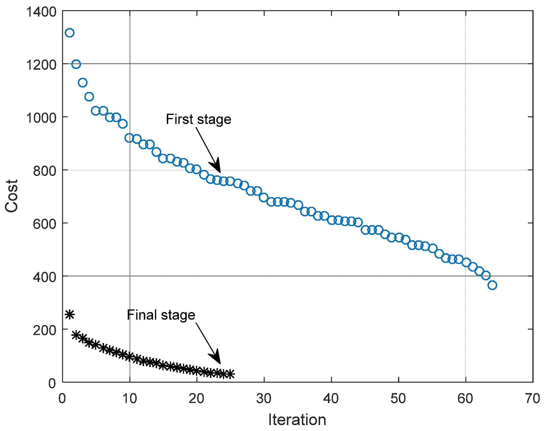
Figure 2 shows the minimum cost trajectory of the proposed algorithm for a six step time horizon as an example. In the first stage, the optimization is performed for the generator UC over the time horizon. The number of UC combination is 64 combinations and each data point in the cost trajectory is the minimum value of the optimization for each of the combination. After the optimal load switch combination was determined in the second stage, the generators and the renewables were fine tuned for the cost minimization in the final stage. On the first and the final stage, each LM optimization process is performed iteratively until the function tolerance is smaller than certain threshold value or maximum iteration number is reached.
3. Control Problem Formulation
3.1. Power Balance
A key operational constraint is that of power balance. All power produced and consumed (or stored) must sum to zero as shown in:
where is the power delivered by the diesel generator in Watts, is the rate of fuel consumption in L/s, is the power delivered by the photovoltaic and the wind turbine generator, is the power consumed by the BESS which can be positive or negative, and and are power consumed by the critical and non-critical loads respectively. represents line loss in the microgrid.
The diesel generator converts chemical energy from diesel fuel into electrical power. The conversion is subject to the efficiency of the engine and generator. For the MPC approach, the system behavior will be optimized over longer time scales, allowing the fast dynamics to be neglected. Thus, neglecting the combustion delay and ramp up/down times, the quasi-steady state electrical power generated by the diesel generator is given by:
where is the efficiency of conversion, is the energy density of the fuel in Joules/L and is the power in Watts needed to maintain the generator in idle at the designated speed. Thus, even though no electrical power is generated, the generator (if it is running) will still incur the cost of fuel consumption to maintain the idle. The generator also has a maximum output power given by the equipment rating .
The power generated by the wind turbine is a function of wind speed and orientation as well as of operator curtailment action. Herein, it is assumed that the wind turbine will operate at maximum power unless curtailed, thus it is modeled as a constrained input where is governed by the weather condition.
The SOC is computed according to the familiar expression given as:
where .
Additional loss or leakage terms may be considered and added to equations (4) or (6). However, these were omitted herein for simplicity. The critical load should be served at any cost without interruption; thus, serving the critical load is an operational constraint. However, the non-critical load is adjustable by the operator from zero up to . The decision variables for the load switches and the generators, which are discrete-valued, introduce nonlinearities into the system. Herein, it is noted that since the generator may be on or off, and since there is a bias term , the fuel consumption is given by:
where , is a decision variable that designates whether the generator is on or off. To aid in solving the optimization problem to be introduced, the variable may be relaxed to which is called the embedded switch state [22,25]. This variable is interpreted as a duty ratio when is not in binary states. Likewise, is replaced with which is the embedded generator power and represented as:
Relaxing the variable improves the ability to solve the problem; however, it results in a new constraint:
After the optimization is solved, the optimal and are interpreted as the generator being on for at a power level of and off for where marks the beginning of the interval and marks the end of the interval.
3.2. Single-Step MPC
A flexible cost function formulation is defined based on the weighted sum of several terms, each representing a different operational objective. The cost function is given by:
where are weighting factors for the squared error of the BESS SOC from desired reference, the deviation of the non-critical load from desired nominal, the curtailment of wind power (it is assumed that in most circumstances), and the use of fuel respectively. These weights are selected to represent a monetary cost or a relative monetary cost (i.e., relative to fuel cost). In addition, tends to favor steady fuel use rather than sporadic or variable use. Finally, weights the deviation in desired dispatch ratio where is set based on some user criteria, and thus captures the cost of starting and stopping the generator.
The cost function may be minimized using a sequential nonlinear program (NLP) which iteratively solves for the optimal power response from each component for some finite time period so as to minimize the value of the cost function subject to constraints. The optimization problem is expressed as:
Selection of the weights in the cost function requires some knowledge of system cost. It is often a challenge to assemble this information, but if the cost is monetary, it may be determined from user agreements with customers, cost of fuel, etc. The cost of curtailing power, for example, is typically the market price for the energy curtailed. In practice, these cost terms are best represented using a 1-norm. However, a quadratic performance index was selected herein to aid in the development of a custom optimization algorithm. Optimization algorithms that benefit from Newton-Raphson-like schemes are easier to develop than those based on the 1-norm. As a starting point, the weights of the cost function may be selected by normalizing the cost of one term relative to another such as 5% SOC error costs as much as shedding the non-critical load.
3.3. Multi-Step MPC
In this section, the one-step MPC control is generalized to a multi-step MPC control. For compactness, the control u and state x are substituted for the power and energy terms used in Section 3.2 using the definitions in Section 2.2. This required some reformulation, but remains consistent with the original approach. Specifically, the problem is formulated using an affine-linear state-space model given by:
where x is the continuous time state, u is the control input as described in Section 2.2, and are time-invariant continuous time state space matrices, and is a vector of time-varying quantities. A linear quadratic cost function is given by:
where is the error state with given as the reference value, is a column vector of weights. Since the MPC control requires a discrete-time formulation, Equation (12) is rewritten as:
where the matrices , and are discrete time matrices. Herein, the Forward Euler method is employed, which is defined simply as:
where T is the time step.
The predicted trajectory of the system is computed over several time steps using this discrete-time model; specifically, each value of the state may be computed in the future using the initial condition and the control policy over N time steps:
It is convenient to modify Equation (16) such that the error state is solved for directly as follows with the more compact formulation shown below, where the overbar designates a matrix or vector with several time steps worth of system information:
Similarly, the cost function is represented in a discrete-time formulation and may be computed using the initial condition and the control policy as:
where .
The Q and R matrices contain the weighting terms . The and matrices are herein selected to be consistent with trapezoidal integration; specifically:
However, since the inputs are assumed to be applied using zero-order hold, trapezoidal integration of the control cost is simply:
From equations (16) and (17), it can be shown that the gradient and Hessian for the cost function are given by:
These terms are used directly in the modified LM iteration described by (3). Note that the Hessian remains constant, but the gradient must be recalculated each time step. Changes in the gradient, however, depend only on the initial condition and the input vector .
4. Case Study
The proposed MPC-based energy management algorithm was demonstrated on a microgrid model in real-time simulation for a one-day scenario. In this scenario, the microgrid is islanded (such as a military FOB) the diesel fuel supply is limited, and an effort is made to extend run-time through optimal use of energy resources, including renewables. The results were used to measure the performance of the optimizer and the effect of forecasting error on the microgrid. In this context, good tolerance to forecasting error is a measure of robustness. The energy management algorithm must make critical decisions surrounding diesel generator operations and support of critical and noncritical load demands. One day uEMS tests pertaining to fuel consumption minimization for a given load demand of the islanded microgrid were performed in a real-time simulation environment, with field data that included load demand, insolation, and wind speed profiles. In addition, the performance metric was developed for the scenario based on the served load demand.
Microgrid Configuration
The microgrid EMS (μEMS) was tested using a real time digital simulation system. The system comprises a real time digital simulator for running the microgrid model in real-time, a PXI platform for a μEMS, and an analog-to-digital conversion (ADC) interface. The ADC interface converts analog measurement data from the simulator for inputs to the μEMS and also for analog output from the μEMS. The μEMS receives the microgrid status such as generator outputs, load demands, breaker status through ADC interface and uses the status information to calculate optimal dispatch. The μEMS samples the output of the diesel generators and their fuel consumptions, the load demands, the BESS SOC, and the renewable generation output every 100 ms. The μEMS feeds this data, including the prediction for the load demand and the renewable generation, to the MPC to generate the dispatch command for the diesel generator, the load switches, and the renewable controls of the real time microgrid model.
Figure 3 illustrates the test AC microgrid with 1350 kW peak load and total generation capacity of 2200 kW as indicated in Table 1. The microgrid has ten separate loads, including three critical loads and seven non-critical loads. To maintain focus on islanded microgrid concepts, the microgrid does not connect to an auxiliary power grid or other external power system. Since the proposed MPC algorithm of the μEMS generates control signals for the diesel generators, the load switches and adjusts renewables based on the predicted load demand every 15 min, it is crucial to maintain the SOC at a certain level to compensate for uncertainty, such as prediction error, to maintain the power balance of the microgrid.
5. Real-Time Simulation Result
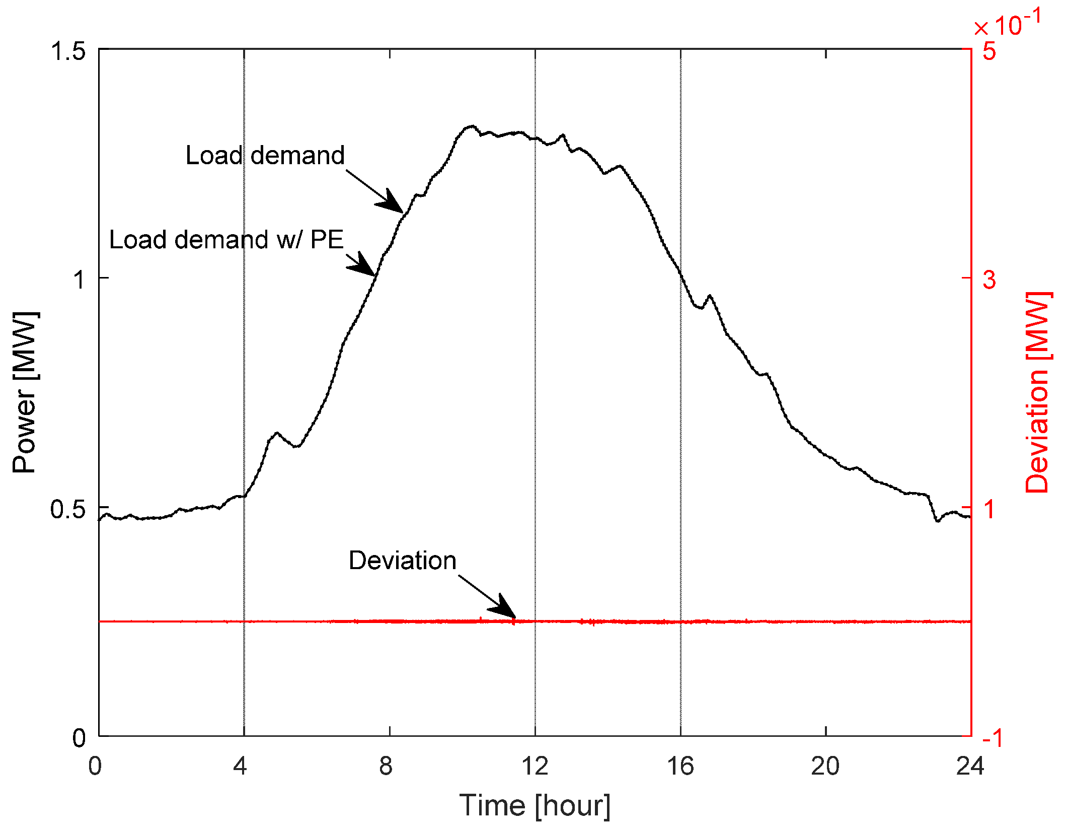
In the case of an islanded microgrid using a diesel generator as the main source, the most important function of the μEMS is to satisfy the load demands that vary with time, using the heterogeneous generation sources. It is shown that the proposed multi-step MPC can effectively manage an islanded microgrid through two real time simulation cases. One scenario considers a case wherein the load demand forecast is perfect, and the other considers a case wherein there is considerable prediction error (PE) between the load prediction and the actual load demand. For the two simulation cases, it is assumed that the fuel of the diesel generator is sufficient. Figure 4 illustrates two scenarios wherein the load predictions are input to the MPC. The solid and dashed lines represent the perfect and the erroneous predictions of the load demand for a day, respectively. The red line represents the discrepancy between the predictions. The negative value of the deviation means the erroneous load prediction is lower than the correct value.
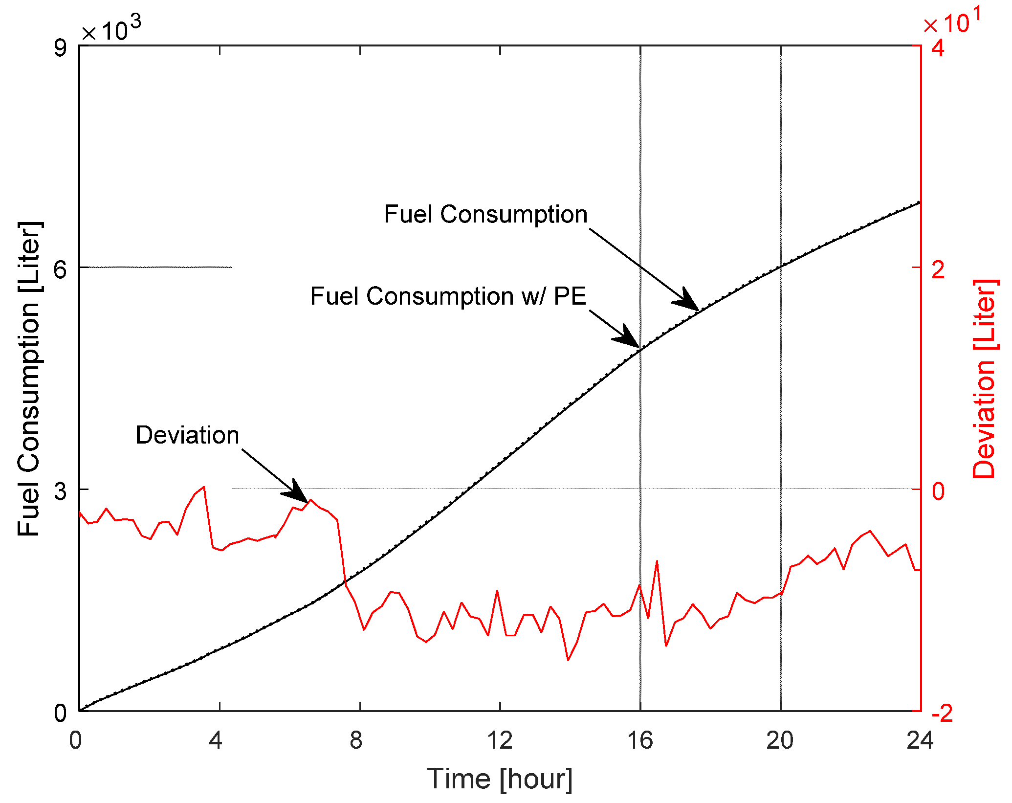
Since the islanded microgrid has limited diesel generation resources and renewable energy sources that cannot be controlled, load shedding can be used to maintain power balance as necessary. However, as it is assumed that the diesel fuel is sufficient to supply the load demand for 24 h, the load shedding cost is heavily weighted to prevent them from shedding for the simulation period. Figure 5 shows the served load demand for 24 h operation of the islanded microgrid. The load demand which is the solid line is the same as the correct prediction in Figure 4. Regardless of the prediction error, the served load of the microgrid with MPC based on the erroneous load demand prediction is the same as that of the correct prediction due to the feedback mechanism in the MPC algorithm that compensates for prediction error. In fact, the differences in the total diesel fuel consumption and the SOC between the two cases (with and without prediction error) are just 0.1% and 0.9% as seen in Figure 6 and Figure 7, respectively.
The load demand is supplied by the diesel generator, the renewables, and a BESS. The deviation between the cases in the diesel generator and the renewables as shown in Figure 8 and Figure 9, respectively, implies that the MPC generated different dispatch commands for the diesel generators due to the prediction error. These dispatch commands resulted in a difference in the diesel generator output and thus a difference in the renewable generation output as shown in Figure 9. When the renewables are curtailed (i.e., limited), the MPC may relax these limits to increase power from renewables or curtail further to reduce power from renewables; in this way, even the renewable energy sources may be modulated to help maintain the SOC to the reference value. However, modifying the renewable generation does not provide as much control authority as it can be limited (i.e., curtailed) but can’t be increased beyond the available resource. The negative deviation in Figure 7 implies that the difference between two diesel generator output values is managed by the BESS and the renewables. The BESS operates as a voltage source and maintains power balance of the microgrid naturally. Therefore, the BESS is critical to the microgrid operation and its SOC should be managed by MPC.
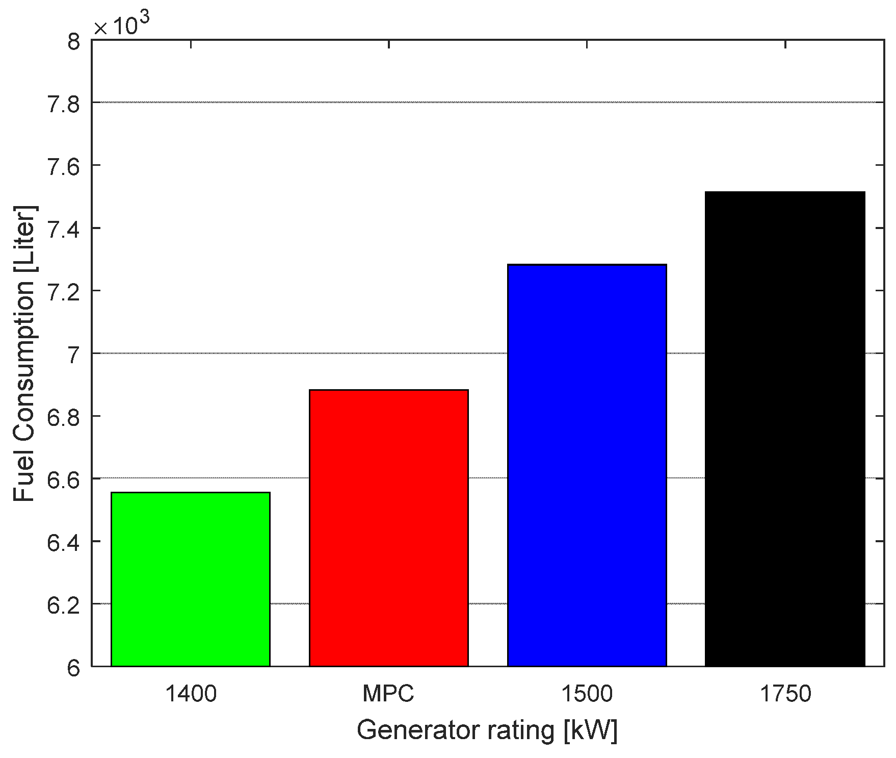
Economics of an islanded microgrid mainly depends on the fuel consumption of diesel generators which are the main power source of the microgrid in general. The fuel consumption mainly depends on the efficiency of the diesel generator and the load demand profile. The efficiency of the diesel generator can be measured by specific fuel consumption (SFC), which is one of the efficiency indicators of the IC engine. It is affected by generator model, rating and loading.
As an ideal reference for comparing fuel consumption, the diesel fuel consumption is calculated for the case where the load demand is the mean of the total diesel power generation in Figure 8 (and with unity load factor for 24 h). As shown in Figure 10 the diesel generators in the test microgrid system, which are controlled by the proposed MPC, consume 5.08% more fuel than the ideal reference, even though the combined SFC of the diesel generators of the test microgrid is much higher than that of the ideal case. Also, considering the reliability of the microgrid, it is not a viable option to use a single diesel generator for the islanded microgrid. Therefore, these results indicate that the MPC can successfully manage multiple diesel generators at near-optimal operating point and provide reliable resource management strategies.
6. Conclusions
In this paper, a multi-step MPC algorithm is proposed and implemented in real-time simulation. The control optimization problem converges to solution for a horizon of 12 time steps of 15 min each, resulting in a time horizon of 180 min. The optimization considers energy costs, and generator and battery depreciation using typical parameter values. The case study with real-time simulation shows that the proposed algorithm works well to provide optimal control for renewable sources, diesel generators, and loads with minimal impact from erroneous load demand prediction to the tracking performance of the algorithm.
Acknowledgments
This work (NRF-2015R1A2A2A01005497) was supported by Mid-career Researcher Program through NRF grant funded by the MEST.
Author Contributions
The research presented in this paper was a collaborative effort among all authors. All authors developed the methodology, conducted the simulation, discussed the results and wrote the paper.
Conflicts of Interest
The authors declare no conflict of interest.
References
- Lasseter, B. Microgrids distributed power generation. In Proceedings of the IEEE Power Engineering Society Winter Meeting, Columbus, OH, USA, 28 January–1 February 2001; Volume 1, pp. 146–149. [Google Scholar]
- Bower, W.; Ton, D.; Guttromson, R.; Glover, S.; Stamp, J.; Bhatnagar, D.; Reilly, J. The Advanced Microgrid: Integration and Interoperability; Technical Report, SAND2014-1535; Sandia National Laboratories: Albuquerque, NM, USA, 2014.
- Arefifar, S.A.; Mohamed, Y.A.; El-Fouly, T.H. Optimum Microgrid Design for Enhancing Reliability and Supply-Security. IEEE Trans. Smart Grid 2013, 4, 1567–1575. [Google Scholar] [CrossRef]
- Johnson, J.; Ellis, A.; Denda, A.; Morino, K.; Shinji, T.; Ogata, T.; Tadokoro, M. PV Output Smoothing Using a Battery and Natural Gas Engine-Generator; Technical Report, SAND2013-1603; Sandia National Laboratories: Albuquerque, NM, USA, 2013.
- Wilson, D.G.; Neely, J.C.; Cook, M.A.; Glover, S.F.; Young, J.; Robinett, R.D. Hamiltonian Control Design for DC Microgrids with Stochastic Sources and Loads with Applications. In Proceedings of the International Symposium on Power Electronics, Electrical Drives, Automation and Motion, Ischia, Italy, 18–20 June 2014. [Google Scholar]
- Olivares, D.E.; Mehrizi-Sani, A.; Etemadi, A.H.; Canizares, C.A.; Iravani, R.; Kazerani, M.; Hajimiragha, A.H.; Gomis-Bellmunt, O.; Saeedifard, M.; Palma-Behnke, R.; et al. Trends in microgrid control. IEEE Trans. Smart Grid 2014, 5, 1905–1919. [Google Scholar] [CrossRef]
- Olivares, D.E.; Cañizares, C.A.; Kazerani, M. A centralized energy management system for isolated microgrids. IEEE Trans. Smart Grid 2014, 5, 1864–1875. [Google Scholar] [CrossRef]
- Teleke, S.; Baran, M.; Bhattacharya, S.; Huang, A. Rule-base control of battery energy storage for dispatching intermittent renewable sources. IEEE Trans. Sustain. Energy 2010, 1, 117–124. [Google Scholar] [CrossRef]
- Shahidehpour, M.; Khodayar, M. Cutting campus energy costs with hierarchical control: The economical and reliable operation of a microgrid. IEEE Electr. Mag. 2013, 1, 40–56. [Google Scholar] [CrossRef]
- Jaganmohan, R.Y.; Pavan, K.Y.V.; Sunil, K.V.; Padma, R.K. Distributed ANNs in a layered architecture for energy management and maintenance scheduling of renewable energy HPS microgrids. IEEE Trans. Ind. Electr. 2011, 58, 316–328. [Google Scholar]
- Bunker, K.; Doig, S.; Hawley, K.; Morris, J. Renewable Microgrids: Profiles from Islands and Remote Communities across the Globe; Rocky Mountain Institute and Carbon War Room: Basalt, CO, USA, 2015. [Google Scholar]
- De Souza Ribeiro, L.A.; Saavedra, O.R.; de Lima, S.L.; de Matos, J.G. Isolated Micro-Grids with Renewable Hybrid Generation: The Case of Lençóis Island. IEEE Trans. Sustain. Energy 2011, 2, 1–11. [Google Scholar]
- Barklund, E.; Pogaku, N.; Prodanvic, M.; Hernandez-Aramburo, C.; Green, T.C. Energy management in autonomous microgrid using stability-constrained droop control of inverters. IEEE Trans. Power Electr. 2008, 23, 2346–2352. [Google Scholar] [CrossRef]
- Morais, H.; Kádár, P.; Faria, P.; Vale, Z.; Khodr, H. Optimal scheduling of a renewable micro-grid in an isolated load area using mixedinteger linear programming. Renew. Energy 2010, 35, 151–156. [Google Scholar] [CrossRef]
- Wang, C.; Hashem, M. Power management of a stand-Alone wind/photovoltaic/fuel cell energy system. IEEE Trans. Energy Convers. 2007, 23, 957–967. [Google Scholar] [CrossRef]
- Hernandez-Aramburo, C.; Green, T.; Mugniot, N. Fuel consumption minimization of a microgrid. IEEE Trans. Ind. Appl. 2005, 41, 673–681. [Google Scholar] [CrossRef]
- Ross, M.; Hidalgo, R.; Abbey, C.; Joos, G. Energy storage system scheduling for an isolated microgrid. IET Trans. Renew. Power Gener. 2011, 5, 117–123. [Google Scholar] [CrossRef]
- Parisio, A.; Rikos, E.; Glielmo, L. A model predictive control approach to microgrid operation optimization. IEEE Trans. Control Syst. Technol. 2014, 22, 1813–1827. [Google Scholar] [CrossRef]
- Nicolao, G.; Magni, L.; Scattolini, R. Stability and robustness of nonlinear receding horizon control. In Nonlinear Model Predictive Control; Springer: Basel, Switzerland, 2000; pp. 3–22. [Google Scholar]
- Liao, G.-C. Solve environmental economic dispatch of smart microgrid containing distributed generation system—Using chaotic quantum genetic algorithm. Electr. Power Energy Syst. 2012, 43, 779–787. [Google Scholar] [CrossRef]
- Takeuchi, A.; Hayashi, T.; Nozaki, Y.; Shimakage, T. Optimal scheduling using metaheuristics for energy networks. IEEE Trans. Smart Grid 2012, 3, 968–974. [Google Scholar] [CrossRef]
- Logenthiran, T.; Srinivasan, D. Short term generation scheduling of a microgrid. In Proceedings of the IEEE Region 10 Conferenced, Singapore, 23–26 November 2009. [Google Scholar]
- Camacho, E.; Carlos, B. Model Predictive Control, 2nd ed.; Springer: New York, NY, USA, 2007. [Google Scholar]
- Allgöwer, F.; Findeisen, R.; Nagy, Z.K. Nonlinear model predictive control: From theory to application. J. Chin. Inst. Chem. Eng. 2004, 35, 299–315. [Google Scholar]
- Mayhorn, E.; Kalsi, K.; Elizondo, M.; Zhang, W.; Lu, S.; Samaan, N.; Butler-Purry, K. Optimal control of distributed energy resources using model predictive control. In Proceedings of the IEEE Power and Energy Society General Meeting, San Diego, CA, USA, 22–26 July 2012. [Google Scholar]
- Palma-Behnke, R.; Benavides, C.; Lanas, F.; Severino, B.; Reyes, L.; Llanos, J.; Sáez, D. A microgrid energy management system based on the rolling horizon strategy. IEEE Trans. Smart Grid 2013, 4, 996–1006. [Google Scholar] [CrossRef]
- Sachs, J.; Sawodny, O.A. Two-stage model predictive control strategy for economic diesel-pv-battery island microgrid operation in rural areas. IEEE Trans. Sustain. Energy 2016, 7, 903–913. [Google Scholar] [CrossRef]
- Nguyen, T.A.; Crow, M.L. Optimization in energy and power management for renewable-diesel microgrids using Dynamic Programming algorithm. In Proceedings of the 2012 International Conference on Cyber Technology in Automation, Control, and Intelligent Systems (CYBER), Bangkok, Thailand, 27–31 May 2012. [Google Scholar]
- Pereira, M.; Limon, D.; Alamo, T.; Valverde, L.; Bordons, C. Economic model predictive control of a smartgrid with hydrogen storage and PEM fuel cell. In Proceedings of the IECON 2013—39th Annual Conference of the IEEE Industrial Electronics Society, Vienna, Austria, 10–13 November 2013; pp. 7920–7925. [Google Scholar]
- DeCarlo, R.; Pekarek, S.; Zefran, M. Optimal control of switching/hybrid systems with applications to hybrid electric vehicles, dc-dc converters, and autonomous mobile robots (M-2). In Proceedings of the American Control Conference, St. Louis, MO, USA, 10–12 June 2009. [Google Scholar]
Figure 1.
Functional diagram of multi-step MPC architecture.
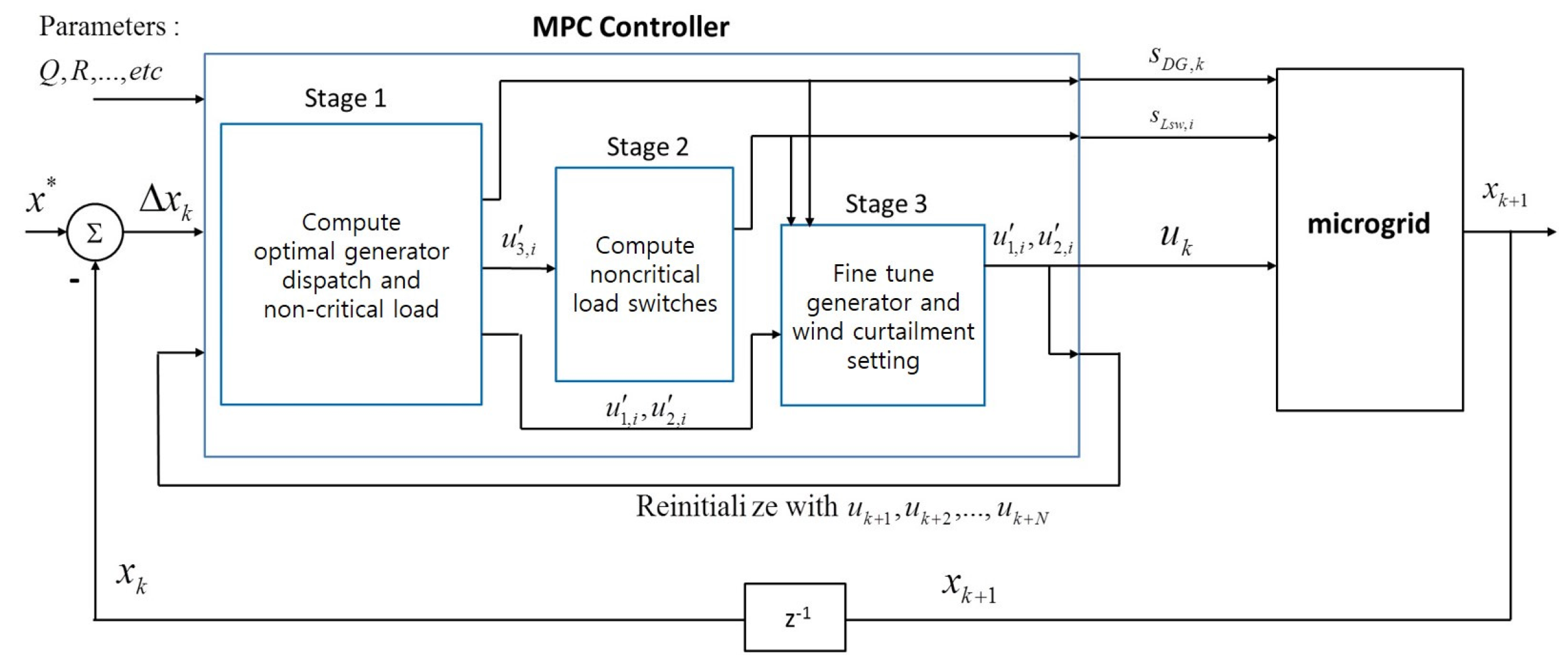
Figure 2.
Cost trajectory example of the proposed algorithm.

Figure 3.
Microgrid model layout.
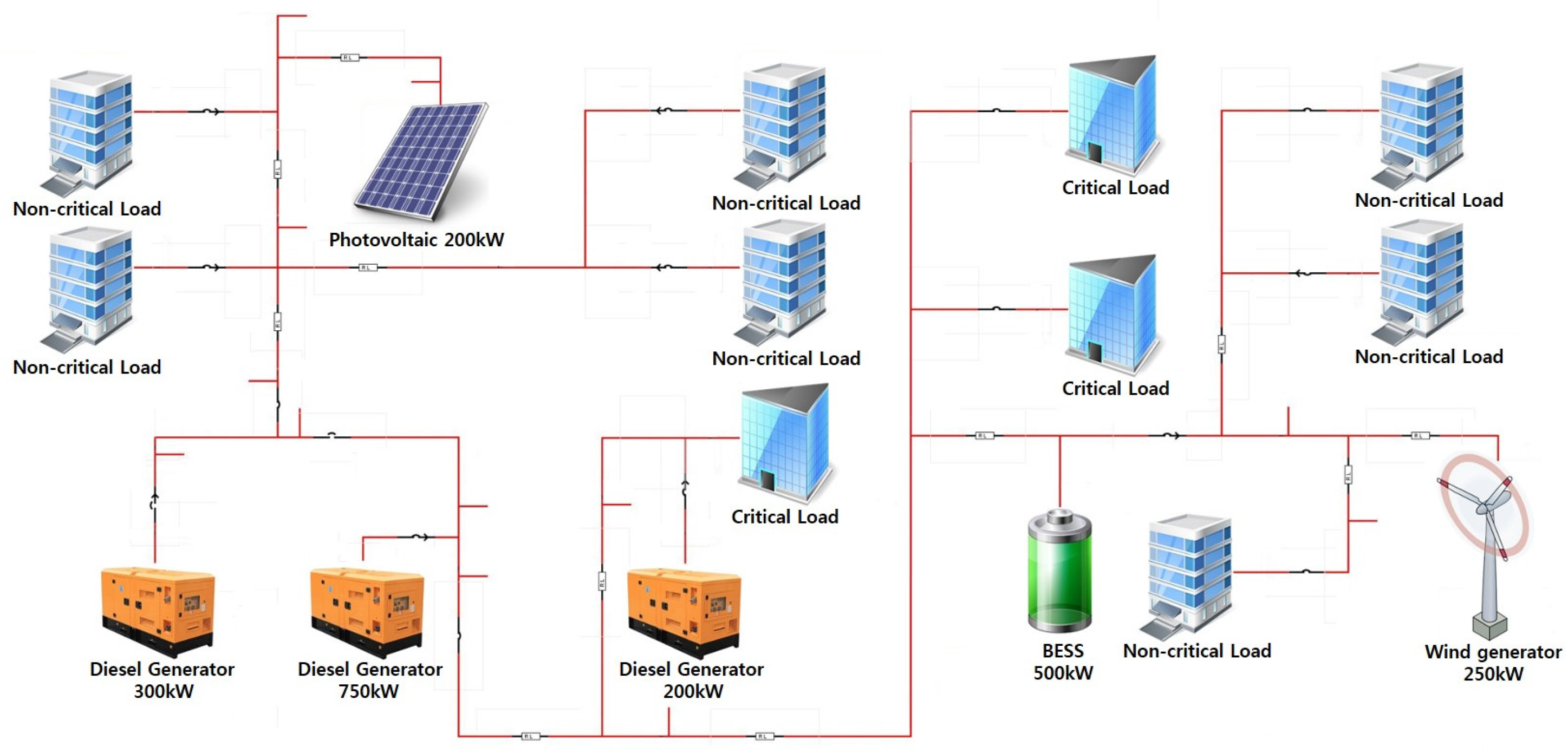
Figure 4.
Predicted load demand for two simulation cases.
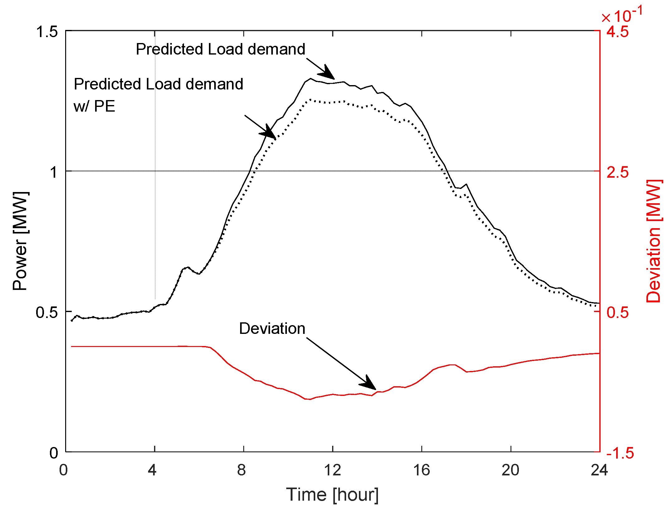
Figure 5.
Served load demand comparison between two cases.

Figure 6.
Fuel consumption comparison between two cases.

Figure 7.
SOC comparison between two cases.
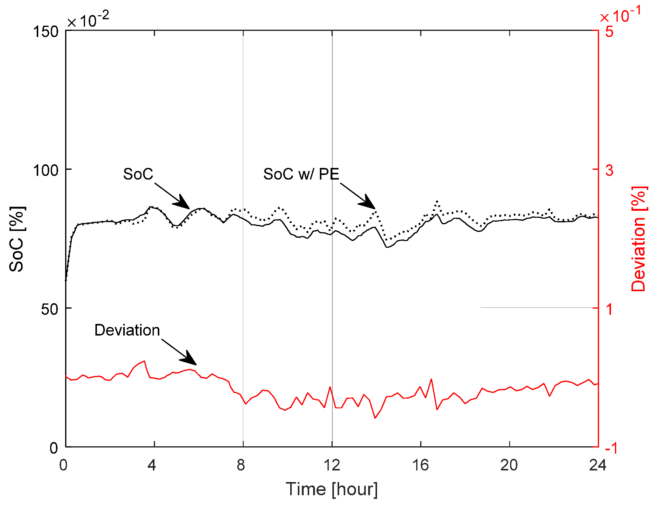
Figure 8.
Diesel generator output comparison between two cases.

Figure 9.
Renewable generation output comparison between two cases.
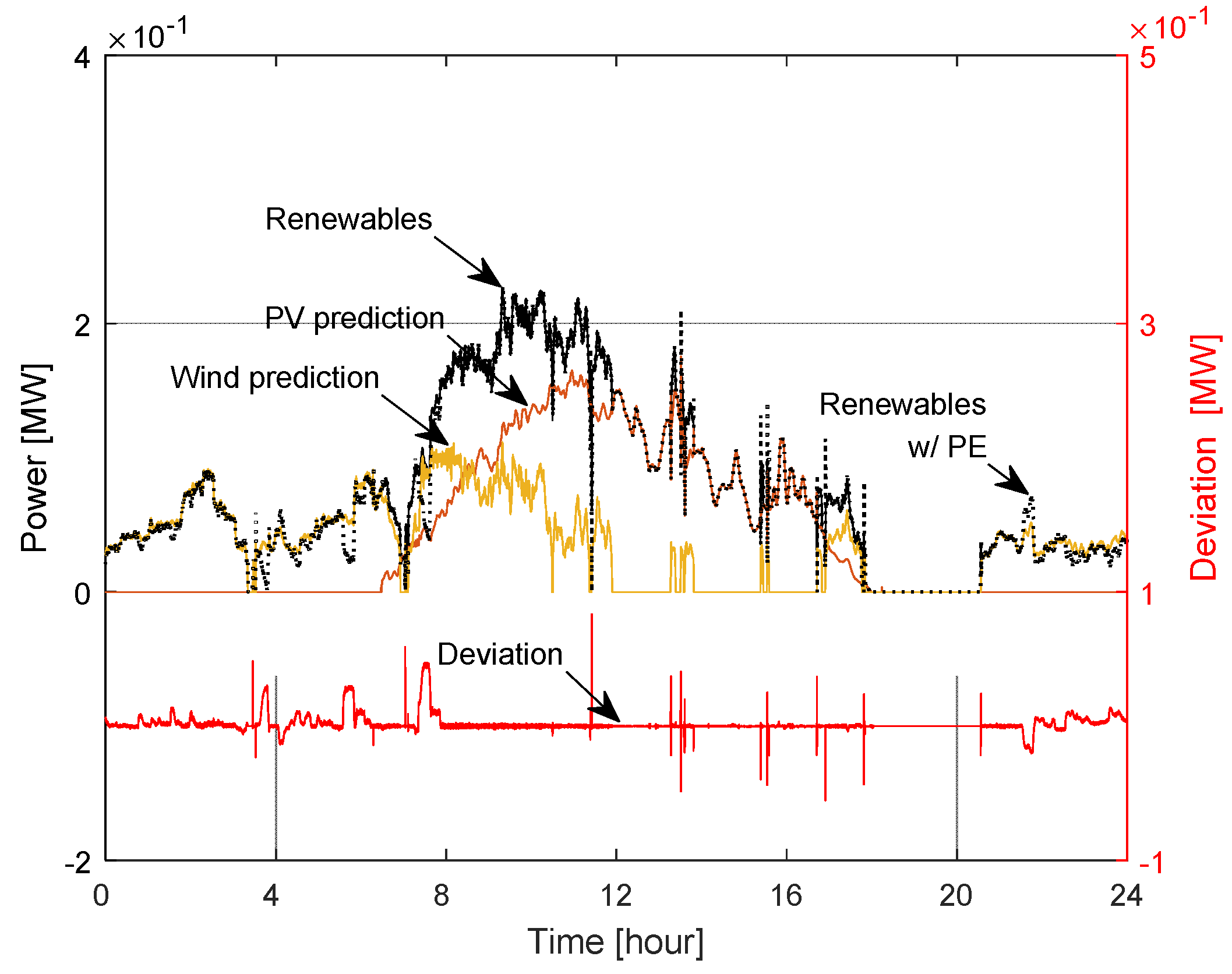
Figure 10.
Diesel generator fuel consumption comparison for 24 h operation.


Table 1.
Microgrid components rating.
| Entity | Voltage [V] | Capacity [kW] |
|---|---|---|
| Diesel | 440 | 200/300/750 |
| BESS | 750 (DC) | 500 (500 kWh) |
| PV | 750 (DC) | 200 |
| Wind | 650 | 250 |
| Feeder | 3300 | 10,000 |
| Loads | 380 | Max 600 each 1 |
1 Transformer rating of the load.
© 2017 by the authors. Licensee MDPI, Basel, Switzerland. This article is an open access article distributed under the terms and conditions of the Creative Commons Attribution (CC BY) license (http://creativecommons.org/licenses/by/4.0/).
Share and Cite
MDPI and ACS Style
Oh, S.; Chae, S.; Neely, J.; Baek, J.; Cook, M. Efficient Model Predictive Control Strategies for Resource Management in an Islanded Microgrid. Energies 2017, 10, 1008. https://doi.org/10.3390/en10071008
AMA Style
Oh S, Chae S, Neely J, Baek J, Cook M. Efficient Model Predictive Control Strategies for Resource Management in an Islanded Microgrid. Energies. 2017; 10(7):1008. https://doi.org/10.3390/en10071008
Chicago/Turabian StyleOh, Seaseung, Suyong Chae, Jason Neely, Jongbok Baek, and Marvin Cook. 2017. "Efficient Model Predictive Control Strategies for Resource Management in an Islanded Microgrid" Energies 10, no. 7: 1008. https://doi.org/10.3390/en10071008
Note that from the first issue of 2016, this journal uses article numbers instead of page numbers. See further details here.