Validating a Wave-to-Wire Model for a Wave Energy Converter—Part II: The Electrical System


1
Centre for Ocean Energy Research, Maynooth University, Maynooth, Ireland
2
Engineering School of Eibar, University of the Basque Country, 20600 Eibar, Spain
*
Author to whom correspondence should be addressed.
Energies 2017, 10(7), 1002; https://doi.org/10.3390/en10071002
Submission received: 24 May 2017
/
Revised: 3 July 2017
/
Accepted: 3 July 2017
/
Published: 14 July 2017
(This article belongs to the Special Issue Marine Energy)
Abstract
:The incorporation of the full dynamics of the different conversion stages of wave energy converters (WECs), from ocean waves to the electricity grid, is essential for a realistic evaluation of the power flow in the drive train. WECs with different power take-off (PTO) systems, including diverse transmission mechanisms, have been developed in recent decades. However, all the different PTO systems for electricity-producing WECs, regardless of any intermediate transmission mechanism, include an electric generator, linear or rotational. Therefore, accurately modelling the dynamics of electric generators is crucial for all wave-to-wire (W2W) models. This paper presents the models for three popular rotational electric generators (squirrel cage induction machine, permanent magnet synchronous generator and doubly-fed induction generator) and a back-to-back (B2B) power converter and validates such models against experimental data generated using three real electric machines. The input signals for the validation of the mathematical models are designed so that the whole operation range of the electrical generators is covered, including input signals generated using the W2W model that mimic the behaviour of different hydraulic PTO systems. Results demonstrate the effectiveness of the models in accurately reproducing the characteristics of the three electrical machines, including power losses in the different machines and the B2B converter.
1. Introduction
Most research effort in wave energy has been mainly focused on maximising the hydrodynamic power absorption of different types of wave energy converters (WECs) from ocean waves. Power from the ocean waves can be absorbed in many different ways, and the different WEC technologies can be categorised into three main groups based on the working principle of each device, as proposed by [1]: oscillating water column (OWC), oscillating-body and overtopping devices. OWC devices comprise fixed or floating structures open below the water surface, where air is trapped above the free surface within the structure. The oscillating motion of the free surface in the structure because of the ocean waves pushes air towards and sucks air from the atmosphere through an air turbine coupled to an electric generator [2]. In the case of oscillating-body devices, in contrast, the action of ocean waves directly moves the device [3,4], which is connected to a power take-off (PTO) system. Finally, overtopping devices capture the water close to the wave crest when it breaks against a structure that includes a relatively large reservoir. A hydraulic pump coupled to an electric generator installed underneath the reservoir converts the potential energy of the stored water into electricity [5].
In the case of oscillating-body WECs, hydrodynamic power is given by the multiplication between the device velocity (), induced by the excitation force (), and the PTO force () and can be maximised subject to design limitations by means of different control strategies [6], including advance control algorithms, such as model predictive control [7] or pseudo-spectral methods [8]. However, the vast majority of the studies in the literature either significantly simplify or completely neglect the PTO system (including control inputs of the PTO system, represented by , and in Figure 1) when designing the controller [7,8,9,10]. Nonetheless, if wave energy is to become a real competitor in the energy market, it is vital to analyse the power flow through the whole power chain, from the waves to the electricity grid, in order to maximize the final energy generated.
To that end, mathematical models that include all of the necessary components of the conversion stages from ocean waves to the electricity grid, known as wave-to-wire (W2W) models, are vital. Such W2W models should include balanced parsimonious models for each stage (including nonlinear dynamics if required and considering the constraints and losses of each component), meaning that the level of detail included in the sub-models for the different stages of the W2W model is balanced. The most important aspects to be considered when modelling W2W models are reviewed in [11] for several different PTO systems (pneumatic [12], hydraulic [13], or a mechanical transmission system [14] coupled to a rotational generator, or a direct drive system with a linear generator [15]), which have been suggested in the literature for different WECs.
The W2W model validated in this paper is a combination of inter-connected sub-models, as shown in Figure 1, where the excitation force is . The outputs for each sub-model are a function only of the inputs taken from the preceding and/or following sub-models. In addition, by implementing multirate time-integration schemes [16,17], each sub-model can use a different time step, which enables one to use the appropriate time step in each sub-model.
The large number of components included in W2W models makes the validation of W2W models, as a whole, quite challenging, mainly due to the complexity and costs of building a physical model that incorporates all of the necessary components. Therefore, the authors propose to accomplish the validation by separately validating each conversion stage of the model, which, in fact, is consistent with the way the model is designed.
The hydrodynamic model of the absorption stage is validated against high-fidelity software in [18], where a heaving point absorber is examined when moving with and without control. The validation of the mathematical models for the transmission, generation and conditioning stages is divided into two parts and is presented as a series of two papers. The first paper (Part I) presents the validation of the transmission stage [19], and the second paper (Part II), the present paper, shows the validation for the generation and conditioning stages, as highlighted in Figure 1.
Although specific W2W models can be designed for different PTO systems, all WECs with the purpose of generating electricity require electric generators, either linear [20,21] or rotational [22,23]. Hence, the model for the electric generator is an essential part of any W2W model for electricity-generating WECs, regardless of the type of PTO system. Rotational electric generators are most widely used in WECs, mainly because of their popularity in other renewable energy applications, such as wind turbines, and are off-the-shelf components. In addition, linear generators, despite their potential for high efficiency performance [24], have been shown to be highly challenging in keeping the required air gap without using robust supporting structures, which considerably reduces the power-weight ratio [25].
In a wide majority of PTO configurations suggested by different WEC developers, three electric generators have been used: a squirrel-cage induction generator (SCIG) [22], a permanent magnet synchronous generator (PMSG) [23] and a doubly-fed induction generator (DFIG) [15]. Hence, the validation for these three rotational electric generators and a back-to-back (B2B) power converter is presented in the present paper.
The remainder of the paper is organised as follows: mathematical models are presented for the three electric generators, including electrical and mechanical equations, in Section 2; the setups of the three experimental platforms including the three electric generators are described in Section 3; the details of the experiments are provided in Section 4; a discussion of the validation is presented in Section 5; and the conclusions are drawn in Section 6.
2. Mathematical Models for Electrical Machines
The dynamics of three-phase electrical machines are typically represented using the two-phase orthogonal rotating reference frame (dq), regardless of the machine topology. Thus, the original alternating-current (AC) signals become direct-current (DC) signals, which simplifies the analysis of the three-phase machines and is convenient for control calculations involving three-phase machines.
The transformation from a three- to a two-phase frame is carried out using the well-known Clarke and Park transformations [26], consecutively. Once all of the necessary variables have been calculated in the dq frame, results can be converted back to three-phase quantities by performing the inverse Park and Clarke transformations.
Mathematical models for the two induction machines, i.e., SCIG and DFIG, are identical except for the rotor voltages and , which are zero for the SCIG and non-zero for the DFIG. Thus, the model for the DFIG is presented in Section 2.1, which can also be used for the SCIG substituting the rotor voltages and by zero in Equations (3) and (4), respectively. The model for the PMSG is presented in Section 2.2.
2.1. Induction Machines
The model for an induction machine is based on the equivalent two-phase circuit illustrated in Figure 2, where the circuits for the direct (d) and quadrature (q) axes are shown in Figure 2a,b, respectively.
Equations of the induction machine model are given [28] as follows:
where , and represent the voltage, current and flux of the direct axis in the stator, respectively. Subscripts s and r are used for the stator and rotor, respectively. and are the resistance of the stator and rotor and and the angular speed of the reference frame and the rotor, respectively. The flux linkages, , as function of currents, are represented as,
where and are the stator and rotor leakage inductances, respectively, and is the mutual inductance.
Hence, the electromagnetic torque developed in an induction machine is given by:
where is the number of poles in the generator.
2.2. Permanent Magnet Machine
The mathematical model for the permanent magnet machine is different from the model for induction machines shown in Section 2.1, due to the major differences in the structure of the electrical machine. Figure 3 illustrates the equivalent circuit for a PMSG, where one can note the substantial differences compared to the equivalent circuit of induction machines shown in Figure 2.
The voltage equations for the stator are [27],
where is the electric angular frequency of the generator and the rotor permanent magnet flux. Electromagnetic torque, in the case of a PMSG, is given [27] by:
Apart from voltage and electromagnetic torque equations, a mechanical equation for the acceleration of the rotor is required, which is identical for both induction and permanent magnet machines. The electromagnetic torque generated in the generator equals the driving torque (including mechanical losses due to friction and windage). Hence, acceleration of the rotor is given as follows,
where J is the rotor mechanical moment of inertia of the generator and is the friction/windage damping. It should be noted that Equation (13) provides the electrical rotor speed, which is not necessarily the same as the mechfanical rotor speed. The electrical speed refers to the frequency, while the mechanical speed corresponds to the actual rotational speed of the shaft. The mechanical speed can be calculated by dividing the electrical speed by the number of pole pairs.
2.3. Back-To-Back Power Converter
Electric generators can be connected to the electricity grid directly (operating at fixed speed) or using a B2B power converter (operating at variable speed) that includes two inverters, a generator-side (GenSI) and a grid-side inverter (GridSI), linked through a smoothing DC line with a capacitor, as illustrated in Figure 4.
The inverters of the B2B power converter allow for the control of the speed and air-gap flux in the electric generator and the output power to be delivered into the grid. However, the operating conditions of the electric generators tested in this paper are limited to sub-synchronous speeds, due to the limitations of the experimental platform, as described further in Section 4. Therefore, the air-gap flux is assumed to be constant, and the GenSI controller only controls the speed of the generator. Hence, reference signals for each inverter, reference speed () and DC voltage (), are given to the corresponding controllers, which are converted into voltage pulses for the inverters by means of the pulse width modulators (PWM), as shown in Figure 4.
Ideally, the mathematical model of an inverter, either GenSI or GridSI, includes the operation of the power switches, reproducing the pulses generated in the PWM units. Despite the accuracy used to define and generate the switching instants in the PWM, it is well known that an inherent waveform distortion occurs in the PWM units (due to switching operations), generating an output voltage signal that necessarily contains harmonics, unless some technique is used to eliminate such harmonics [29]. To examine the performance of the electric generators, however, such harmonics can be neglected [30].
In addition, due to the high switching frequencies of PWM units (typically between 1–20 kHz in applications related to the control of AC motors), simulations require a very refined time step (1–10 s), which increases computational requirements to prohibitive levels. Therefore, the mathematical model of the B2B power converter presented in this paper neglects the harmonics generated by the PWM unit and considers only the fundamental frequency of the voltage signals delivered into the electric generator and the electricity grid, referred to as and in Figure 4, respectively. Therefore, the PWM block in Figure 4 is a simple unitary gain, meaning that reference voltage signals obtained in the controllers and the actual voltage signals are identical ( and , in Figure 4).
The DC-link between the GenSI and the GridSI can comprise a single capacitor or a bank of capacitors. These capacitors can absorb the instantaneous active power fluctuations, smoothing the output power flow, and work as a voltage source for the converters. Variations of the DC voltage on the capacitor can be obtained as follows [31],
where and are the currents at the grid and generator side of the capacitor in the DC link, respectively, C is the capacitance of the capacitor(s) at the DC-link and is the voltage in the capacitor(s).
2.4. Power Losses
Modelling the power losses in electric generators and power converters is vital to accurately evaluate the final power generation. Electric generators are generally designed to minimise losses at full-load conditions, but losses increase substantially at part-load operations. Power losses may arise from different sources, and it is not always straightforward to include them in the mathematical model.
More insight to the efficiency characteristics of electrical machines is provided in [32], where losses in the SCIG, PMSG and DFIG, including power converters, are studied.
2.4.1. Electric Machines
Power losses in electric generators appear mainly due to large current requirements, which are manifested as large copper losses. The models described in Section 2.1 and Section 2.2 for induction and permanent magnet machines, respectively, include the most important electric and mechanical dynamics and consider losses due to the Joule effect (i.e., copper losses in the stator and the rotor), core losses (i.e., stray losses) and mechanical losses (i.e., friction and windage losses). However, it should be noted that iron losses are not included in the model, because they are considered negligible [28].
Figure 5 illustrates the losses in the different parts of an electric generator, from the rotor to the stator. Mechanical losses () due to friction and windage can be described as follows,
while copper losses in the rotor () and the stator () are given as,
2.4.2. Power Converters
Power converter units comprise a number of power switches interconnected in a way that allows for the generation of AC signals from DC signals, and vice versa, by switching on and off the power switches.
Energy losses in converters arise from the non-ideal switching and conduction phases, illustrated in Figure 6. Power switches cannot switch on and off instantaneously, and as a consequence, there exits a finite time window, referred to as or for switching on or off, respectively, where the non-zero overlap in time of collector-emitter voltage () and current () happens in the power switch. Figure 6 illustrates the non-zero overlap in time of the voltage and the current and the power losses associated with switching operations in such time windows.
Switching losses, regardless of switching on or off, are commonly expressed as,
where is the switching frequency and is when switching on and when switching off.
Conduction losses, on the other hand, can be calculated as follows,
where is the resistance of the selected power switch. Such conduction losses are constant for the whole period the power switch is conducting, as illustrated in Figure 6.
However, if the operation of power switches in the inverter is not included in the model, as described in Section 2.3, power losses cannot be calculated using Equations (21) and (22). Therefore, another alternative to evaluate power losses in the inverters, via experimental data, is suggested in this paper, as shown in Section 5.2.
3. Experimental Setup
The three electrical machines used for the validation of the mathematical models presented in Section 2.1 and Section 2.2 are installed in the Engineering School of Eibar. The electrical machine is driven, in all of the cases, by a permanent magnet synchronous motor (PMSM) coupled to the rotor of the generator. Only the DFIG is grid connected using a B2B configuration, while the SCIG and the PMSG are connected to a capacitor bank, where energy is stored. That capacitor bank is used as the energy source for the PMSM and as a sink for the energy generated in the generator, forming a closed loop and avoiding the need to dissipate the generated energy.
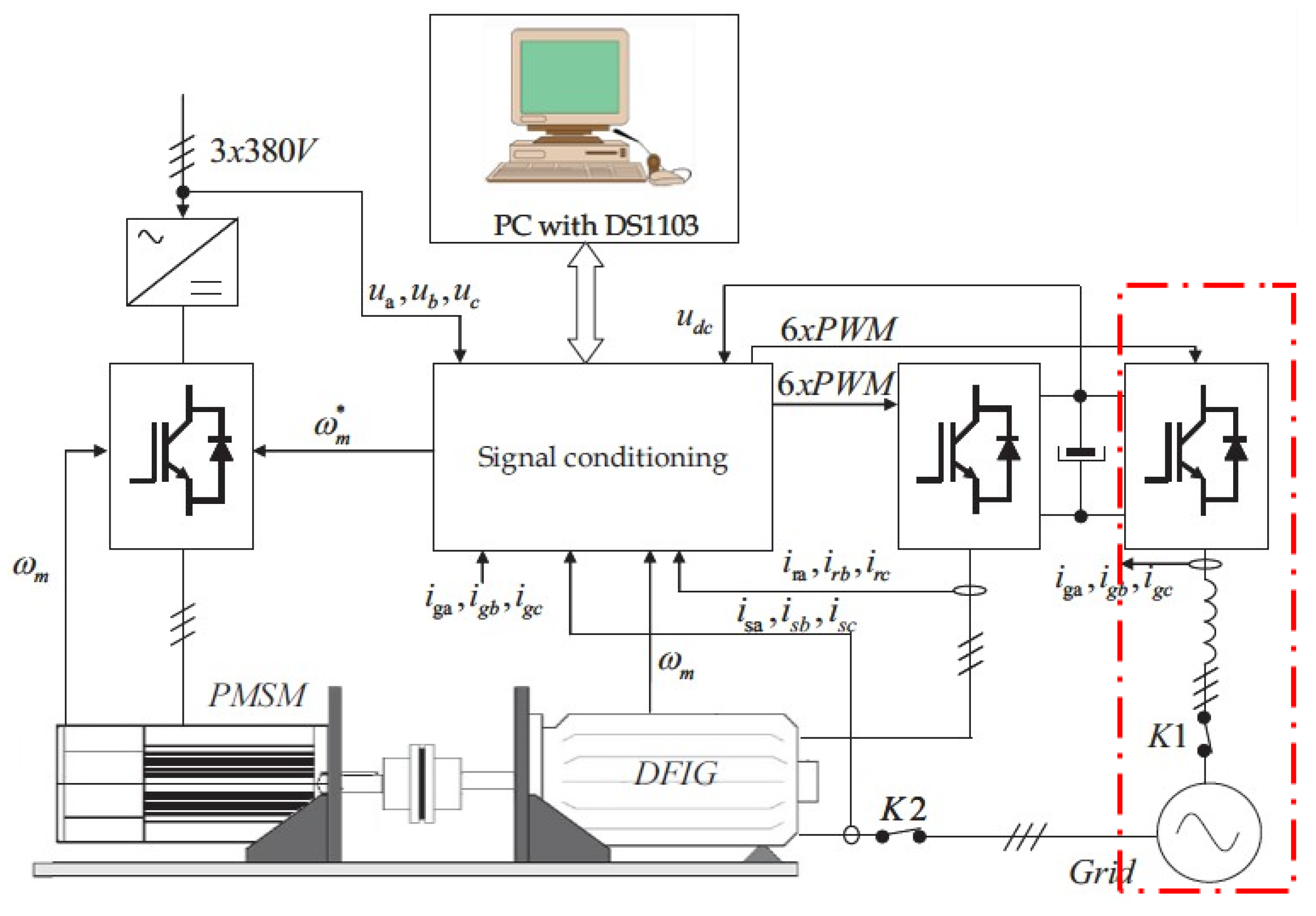
To generate the validation signals, a control platform is required in the experimental setting. The control platform is identical for the SCIG and PMSG and varies slightly in the case of the DFIG. Figure 7 illustrates the diagram of the experimental platform for the DFIG, including the back-to-back converter and the control platform, where u is the voltage, the grid current and subscripts a, b and c represent the three phases of the three-phase representation. In the case of the SCIG and the PMSG, the second inverter of the B2B converter, illustrated inside the red dash-dotted rectangle in Figure 7, does not exist, and the first inverter of the B2B converter is connected to the stator, instead of the rotor. An image of the experimental platform is shown in Figure 8, where all of the components of the diagram in Figure 7 are shown: the PMSM, the DFIG, the control PC with he DS1103 controller board and the GenSI and GridSI, referred to as RSCand GSC, respectively, in Figure 8.
The control platform shown in Figure 7, which has been employed to test several control strategies in the context of wind energy [33,34], includes a PC with MATLAB/Simulink R2007a (Mathworks, Natick, MA, USA) and dsControl 3.2.1 software (dSPACE, Paderborn, Germany), as well as the DS1103 Controller Board (dSPACE, Paderborn, Germany) real-time interface using a dSpace system. The DS1103 Controller Board controls the GenSI and GridSI, generating the space vector PWM pulses with a maximum frequency of 7 kHz (143 s).
The starting sequence of the machines varies for each generator. In the DFIG, the capacitor in the DC-link needs to be charged first. Once the DC-link is charged, the GridSI is connected to the grid by means of connector K1, allowing for DC-link voltage regulation. Voltage in the DC-link must be greater than the peak value of the grid voltage, which is about 540 V for a grid RMS voltage of 380 V. Therefore, the DC-link voltage is set to 570 V in the experiments. After connecting the GridSI to the grid, the stator voltage is synchronised with the grid voltage. This voltage synchronisation is carried out by means of a phase locked loop (PLL), via measurement of the grid side voltage. Finally, the stator is connected to the grid by switching connector K2.
In the SCIG and the PMSG, the capacitor in the DC-link must be charged first as well, but the rest of the starting sequence is significantly different. In fact, the capacitor in the DC-link is a capacitor bank of 3300 F and 1500 F in the SCIG and PMSG, respectively, which is used as the voltage source for the GenSI. In the case of the SCIG, once the DC-link is charged, the rated flux is imposed in the generator via the control platform, so that only after rated flux is established in the generator can the rotational speed regulation start. The PMSG, on the other hand, requires determining the initial position of the rotor before starting. To that end, a brief impulse is introduced to the generator, so that the encoder offset with respect to the position of the rotor can be determined. Hence, the rotational speed of the generator can be regulated using an adequate angle compensation.
All of the ratings and parameters for the SCIG, PMSG, DFIG and inverters are provided in Appendix A in Table A1, Table A2, Table A3 and Table A4, respectively.
4. Experiment Design
The design of the experiments to validate the mathematical models is not a trivial decision. The signals used in the experiments should excite the system over its whole range of operation, so that the experiments cover:
- the response to all of the important frequencies and
- the full input/output signal ranges,
In an efficient way, making a good use of the test time. This is a common issue in system identification [35], where the information of the system’s behaviour for the whole range of possible conditions is essential to accurately identify the parameters of the model. Multi-sinusoids, which contain a set of frequencies, or pseudo-random binary signals, which have a flat frequency spectrum, are typically used for the identification of linear systems [36]. However, nonlinear systems require a full operational range of both frequencies and amplitudes, for which pseudo-random signals with randomly varying amplitudes, also known as random-amplitude random-phase (RARP) sequences, are a good candidate [37].
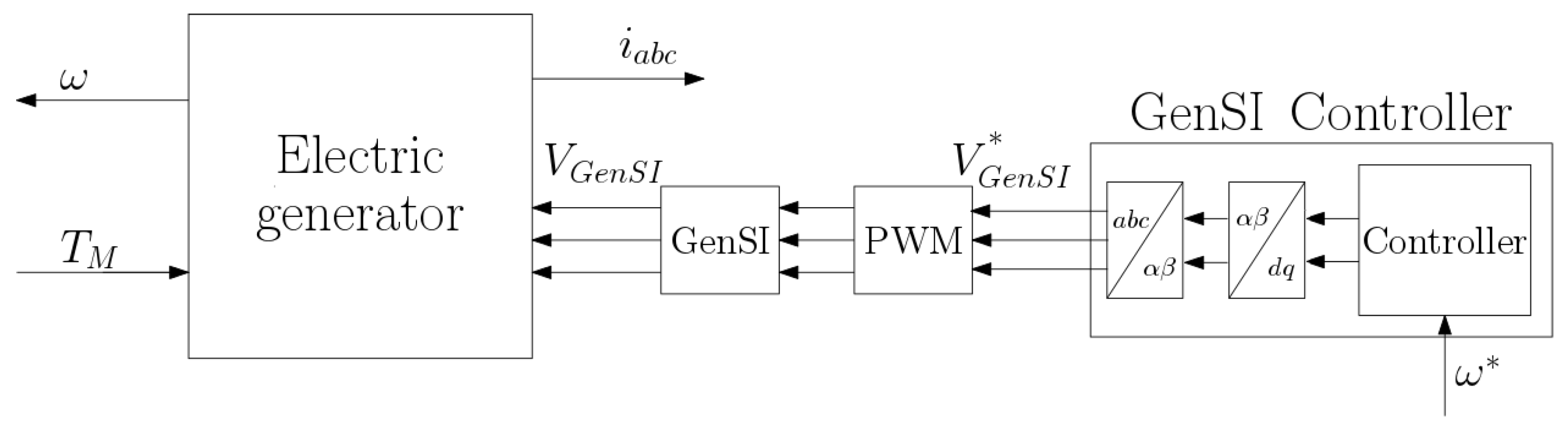
Inputs for the electric generator validation system, which includes the generator, GenSI and the controller as illustrated in Figure 9, are the driving torque () and the reference rotational speed (). Electric generators are used in different types of WECs and coupled to different transmission systems, so the input signals utilised in the validation must cover the operating conditions of electric generators included in any WEC and coupled to any PTO system. The pattern of the input torque signal of the electric generator depends on the configuration of the PTO, regardless of the type of WEC. A PTO system that includes large accumulation systems, such as an overtopping device [38] or any wave-activated device with a hydraulic transmission system that includes large hydraulic accumulators [13,39], provides slowly-varying, smooth torque signals. In contrast, transmission systems directly connected to the electric generator, such as air turbines in oscillating water column devices [40], mechanical systems [14] or hydraulic systems without large accumulators [41] provide highly variable torque signals. Therefore, realistic operational conditions can be categorised in two groups: constant input torque and variable input torque. In some cases, the efficiency of the PTO system is improved by varying the rotational speed of the electrical generator [41], which modifies significantly the behaviour of the electric generator.
Consequently, the experiments utilised for the validation of electric generators to fully cover all of the different possible realistic conditions must include, at least, three different test cases: constant input torque combined with constant rotational speed, variable input torque with constant rotational speed and variable torque with variable rotational speed. However, the amplitude and period of the input signals, for any of the three test cases, may vary considerably depending on the amplitude and period of the input waves. As a consequence, several different experiments should be considered for each test case, resulting in an infeasible number of experiments.
Nevertheless, the full range of different amplitudes and periods can be efficiently covered by the RARP signals. Therefore, the combination of RARP signals and realistic PTO signals based on single input wave conditions can completely cover the operational conditions of any electrical generator coupled to any type of transmission system and WEC with a minimum number of experiments. Hence, six sets of combined torque and speed signals are specified in total for the validation of each machine, three sets based on RARP sequences and another three sets based on realistic PTO signals. In the latter, the realistic PTO is represented by a hydraulic transmission system, and the input signals are generated using a W2W model, as described in Section 4.2. The six sets of inputs are tested in the three different generators presented in Section 3.
4.1. Random Input Signals
The three sets of RARP signals consist of two sets where only one of the inputs varies randomly, while the other remains constant, and a third set where both inputs vary randomly:
- Test 1a: Zero driving torque and varying reference speed.
- Test 1b: Varying driving torque and constant (rated) reference speed.
- Test 1c: Varying driving torque and reference speed, as shown in Figure 10a.
The RARP signals for the first 50 s (out of 200 s) of the Test 1c are illustrated in Figure 10a, for which frequency content and normalized amplitude distribution are shown in Figure 10b,c, respectively. The signal length is chosen to be 200 s, which permits a good coverage of the required amplitude and frequency ranges. Increasing the length of the signals results in a more even coverage of the amplitude range. However, increasing the signals above 200 s, no substantial improvement is seen in the coverage of the frequency and amplitudes. In contrast, the distribution of the frequency content is heavily influenced by the maximum allowable switching period of the signal, which is selected to be 1.4 s [0.7072 Hz] to enable a good coverage of the frequency range, as shown in Figure 10b.
All RARP signals are normalised signals, so that the same inputs can be implemented in different machines by multiplying the normalised signals with the rated torque and speed of the appropriate generator.
4.2. Realistic PTO Input Signals
Realistic PTO input signals are generated using a W2W model, producing input signals that an electric generator would experience when coupled to a realistic hydraulic transmission system, which is, in turn, connected to a WEC. Figure 1 illustrates that the W2W model, where the driving torque is produced by the hydraulic motor and the voltage input is given by the power conversion unit, for which is the control input represented as in Figure 9. The waves implemented in the W2W model are irregular waves generated using a JONSWAP spectrum [42], and a spherical heaving point absorber is used as the WEC.The JONSWAP spectrum is generated for a peak period of 10 s, a shape factor of 1.25, an intensity of the spectrum of 0.0081 and a peak enhancement factor of 3.3.
Several different hydraulic PTO topologies have been suggested in the literature, which can be organised into two main groups [43]: a hydraulic system with high storage capacity (referred to as constant-pressure configuration consP), and a hydraulic system with limited storage using a variable-displacement hydraulic motor (referred to as variable-pressure configuration varP).
These two hydraulic PTO configurations generate different input signals for the electric generator. Hydraulic PTO systems based on the consP configuration use, in general, electric generators operating at constant rotational speed, and the torque generated by the hydraulic motor is practically constant, as shown in Figure 11a. In contrast, the torque signal in the varP case vary significantly, as shown in Figure 11b,c. In addition, PTO systems based on the varP configuration suggested in the literature use electric generators that operate either at constant or variable rotational speed.
Therefore, the three sets of realistic PTO inputs are organised as follows:
In Test 2c, rotational speed follows the profile of the driving torque, but is constrained to the rated rotational speed of the generator, as shown in Figure 11c. Similarly to the RARP signals, realistic PTO signals are also normalised signals, so that they can be used for the validation of the different electric generators.
5. Validation
Electrical and mechanical dynamics of the generators are validated by comparing measurements from real machines to the corresponding output signals from the models. The output signals from the electrical generators, as illustrated in Figure 9, are the rotational speed () and stator currents (). However, the electromagnetic torque, generated power (real and reactive) and power losses in the generators are also compared to study the suitability of the mathematical models.
Different variables from diverse test cases and electrical generators are studied in the present paper. Hence, for the different error measures to be comparable, an error measure that is suitable for all of the variables is required. Normalised measures facilitate the comparison of diverse datasets with different scales, which is necessary in this case. Unfortunately, the popular mean average percentage error (MAPE) metric cannot be employed, since there are values in the datasets that are zero or close to zero, which would imply a division by zero. The normalised root mean square error (NRMSE) could be a suitable candidate. However, because variables vary from zero to the nominal value in some test cases, using a single average value of the whole simulation for the normalisation can bias the error measure. Therefore, the validation is evaluated by means of an alternative normalized root mean square error, known as the moving average normalised root mean square error (MANRMSE), given in Equation (23). Hence, signals are divided into N parts, using a different average value in each part j to normalise the error. The bias of the error measure decreases as N increases, since the average value corresponding to each j part is more representative of the signal values in that j part. However, there is a value of N, after which increasing Ndoes not affect the error measure. That value of N ensures an unbiased error measure, without losing the characteristics of the signals. In the present paper, the error measure was observed to be constant when the signals were divided into more than 40 parts, so was chosen to obtain the fidelity values.
where y is the measured value, the value given by the model, the average value at each part j and n the number of samples in each part. Once the MANRMSEis calculated, the fidelity of the variables from the mathematical model in percentage terms can be obtained as follows,
5.1. Electrical Generator Validation
Fidelity values shown in Table 1 for the SCIG show a good overall agreement between the machine and the mathematical model, where fidelity values above 90% are shown for most of the test cases and variables. Results from the mathematical models, considering all of the variables and test cases, show the ability to reproduce the behaviour of the real machine, as illustrated in Figure 12 for the rotational speed, electromagnetic torque and active and reactive power.
The chaotic behaviour of the real power in Figure 12b corresponds to the abrupt variations of the inputs signals of the test case Test 1c, as shown in Figure 10. Due to these abrupt variations, the generator rapidly varies from operating close to full-load conditions to part-load condition, or vice versa. As a consequence, high power spikes appear, which can lead to high negative power values when the generator requires sucking power from the grid to reach the new operating conditions. However, the measurements of the real machines show considerable high-frequency fluctuations, as illustrated in Figure 12, which reduce the fidelity of the mathematical models for the electric generators. In fact, one can observe, from Figure 12, that such fluctuations are the main difference between the experimental results and the results obtained from the mathematical models.
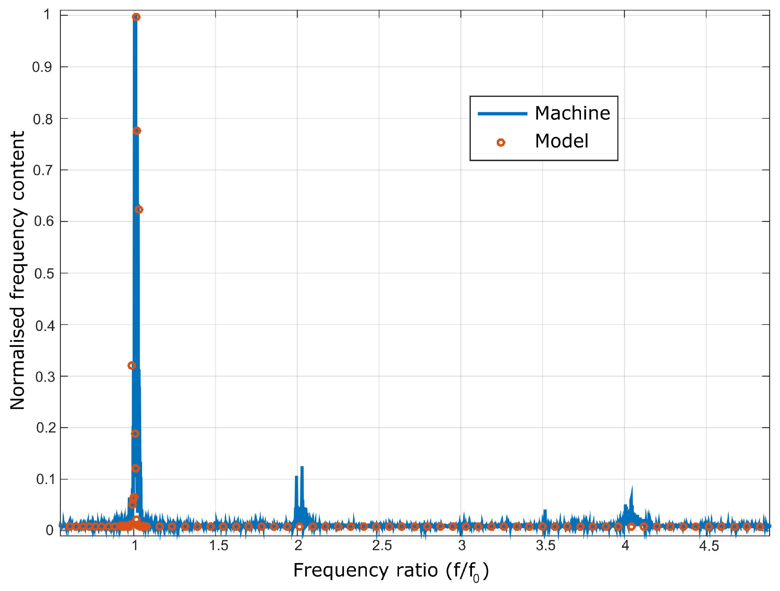
High-frequency fluctuations appear in all of the test cases and variables, except for the rotational speed, as shown in Figure 12, because the inertia of the rotor shaft smooths out the rotational speed signal. The source of these high-frequency fluctuations are likely to be harmonics generated by power converters and the noise of the measurements. Harmonics inserted by power converters include fluctuations of frequency multiplied bythe fundamental frequency, while the noise added by virtue of the sensors includes a random error in the signal [44]. Figure 13 illustrates the frequency content of the stator voltage signal in Test2b, for which the the fundamental frequency is 50 Hz for the whole simulation, because the rotational speed is constant. In addition to the fundamental frequency, one can clearly see the harmonics at twice () and four-times the fundamental frequency (), as well as the noise all over the frequency range in the case of the real machine. The mathematical models described in Section 2, however, do not incorporate switching operations of the power converters, as explained in Section 2.3, and as a consequence, results from the mathematical models show no high-frequency fluctuation, as illustrated in Figure 12. The frequency content associated with the voltage signal of the mathematical model is, indeed, zero far from the fundamental frequency, as shown in Figure 13.
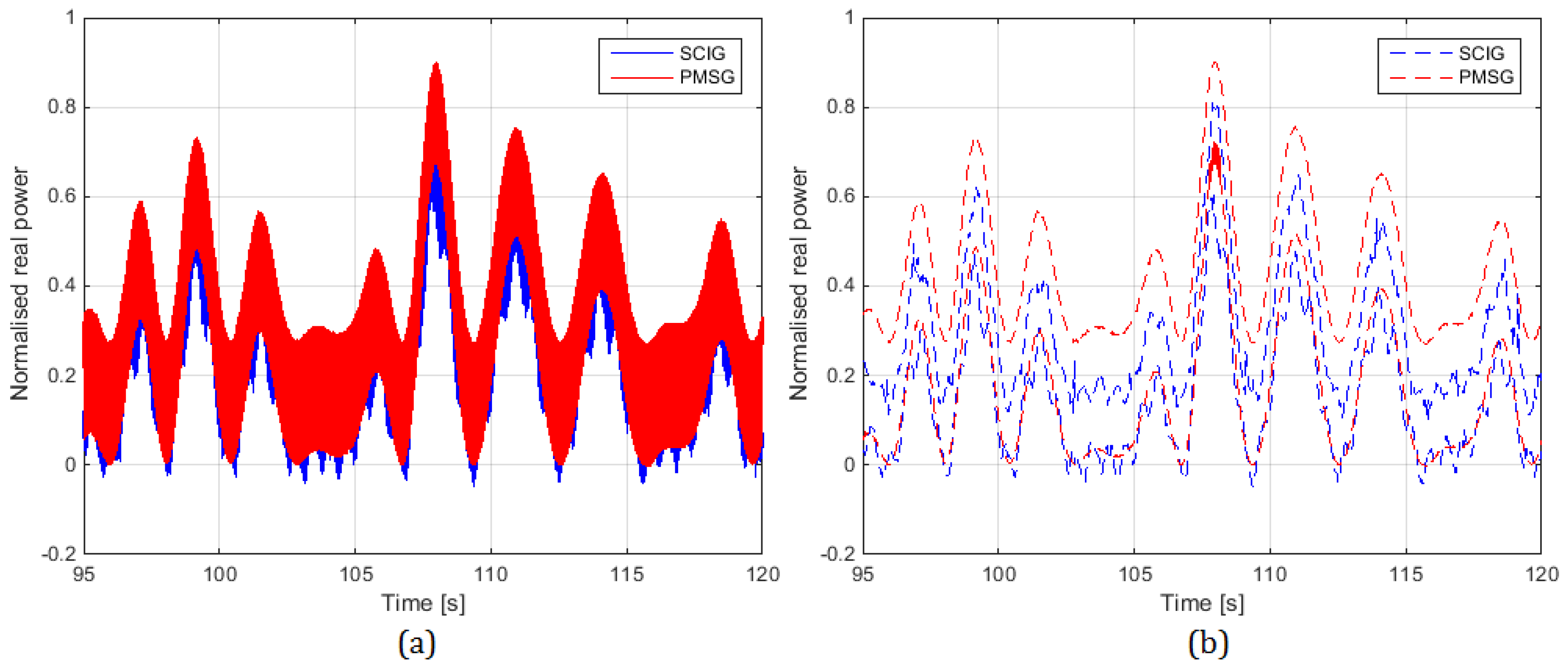
In the case of the PMSG, the fidelity values shown in Table 2 also show good agreement between the mathematical model and the machine, with fidelity values over 90% for most of the test cases and variables. Similarly to the SCIG, the test case Test 2a shows the results of lower fidelity values. However, fidelity values, in general, are lower in the PMSG than in the SCIG. These lower fidelity values are associated with stronger high-frequency fluctuations, as illustrated in Figure 14, where the level of high-frequency fluctuations is compared for the PMSG and the SCIG. Figure 14a illustrates normalised real power values (normalised against rated power), and Figure 14b shows the upper and lower envelopes of the normalized real power signals. The lower envelope for the SCIG and the PMSG in Figure 14b is almost identical, while the upper envelope is considerably higher for the PMSG, which illustrates the larger level of high-frequency fluctuations in the PMSG.
Larger high-frequency fluctuations in the PMSG can also be due to the higher rated rotational speed of the PMSG, which is twice as high as the rated rotational speed of the SCIG. The higher the rotational speed, the higher the frequency, which leads to faster pulses generated by the PWM voltage source converter and, as a consequence, to stronger fluctuations.
Finally, fidelity figures for the DFIG, shown in Table 3, are similar to those obtained for the SCIG, which shows, once again, good agreement between the mathematical model and the machine. Rated power and rotational speed are identical for the SCIG and the DFIG, confirmed by the similar fidelity values.
Apart from the dynamics of the machines, for which the effectiveness of the mathematical models has been demonstrated, accurately estimating power losses of the generator is crucial. Therefore, the efficiency of the machines is studied, comparing efficiency values obtained from the real machines and the mathematical models in the three generators, for the test case Test 1c.
Test 1c is the test case that best covers the whole operational range of the generators, randomly varying rotational speed and driving torque, as shown in Figure 10. Although such random variations of the rotational speed and driving torque are rather unusual in normal operations, the coverage of the full range of operational conditions makes Test 1c especially suitable for the study of efficiency. However, such random variations include abrupt spikes in the power and efficiency signals. In addition, because speed and torque input signals vary randomly, the electric generators operate at high rotational speed and low torque at some points during the simulation, which results in significant efficiency drops.
Therefore, Figure 15a–c illustrate the trend lines of the efficiency signals for the SCIG, PMSG and DFIG, respectively, as a function of the normalised rotational speed, providing satisfactory agreement between the curve of the real machines and the curve of the mathematical models. Efficiency signals are fitted using a power trend line as follows,
where is the trend line, , and are the coefficients of the power function that are identified to fit the data and x is the variable on which the trend line is based, i.e., normalised rotational speed in this case. The coefficients of the power function for each generator are given in Table 4.
5.2. Power Converter Validation
The experiments carried out in the DFIG, since it is grid connected in a B2B configuration, are also used to validate the B2B converter implemented in the mathematical model, as described in Section 2.3, including power losses in the GenSI and GridSI.
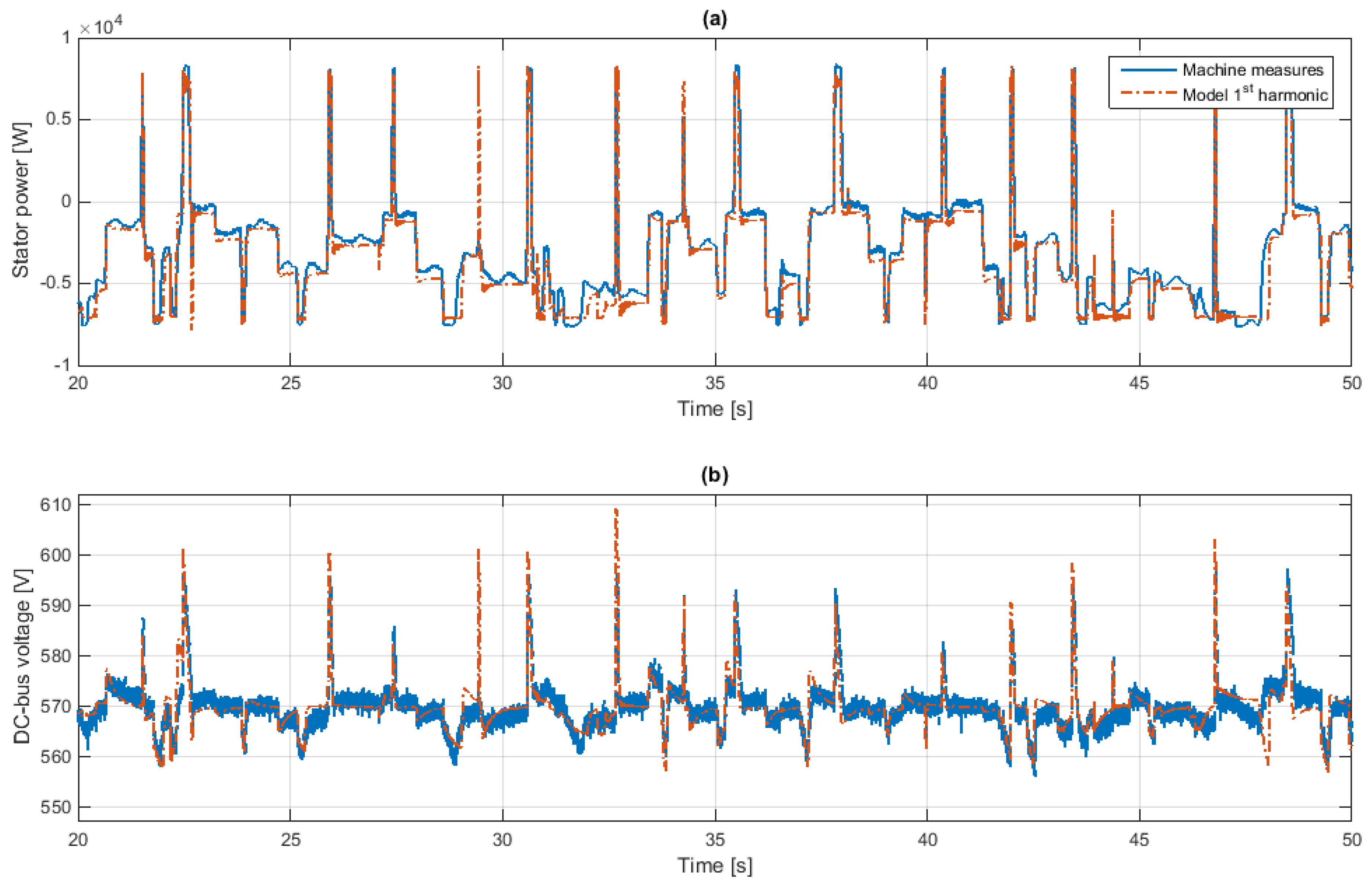
The main objective of the GenSI and GridSI is the control of the electric generator and DC-link voltage, respectively. The ability of the mathematical model to accurately reproduce the effect of the controller in the GenSI is illustrated in Figure 16a for the DFIG and Test 1c and has been demonstrated in Section 5.1 for all of the generators and a wide range of operating conditions. Similar results can be obtained in the case of the GridSI, where the control of the DC-link voltage in the mathematical model is almost identical to the DC-link voltage control in the experimental platform.
Fidelity values, obtained by comparing the DC-link voltage values from the experimental platform and the mathematical model, are presented in Table 5, showing an excellent agreement between the experimental and numerical results. Figure 16b illustrates that agreement for Test 1c.
However, power losses in the power converters can only be studied if the operation of the power switches in the inverters is considered in the model, which are not included in the mathematical models described in Section 2.3, due to the prohibitive computational requirements.
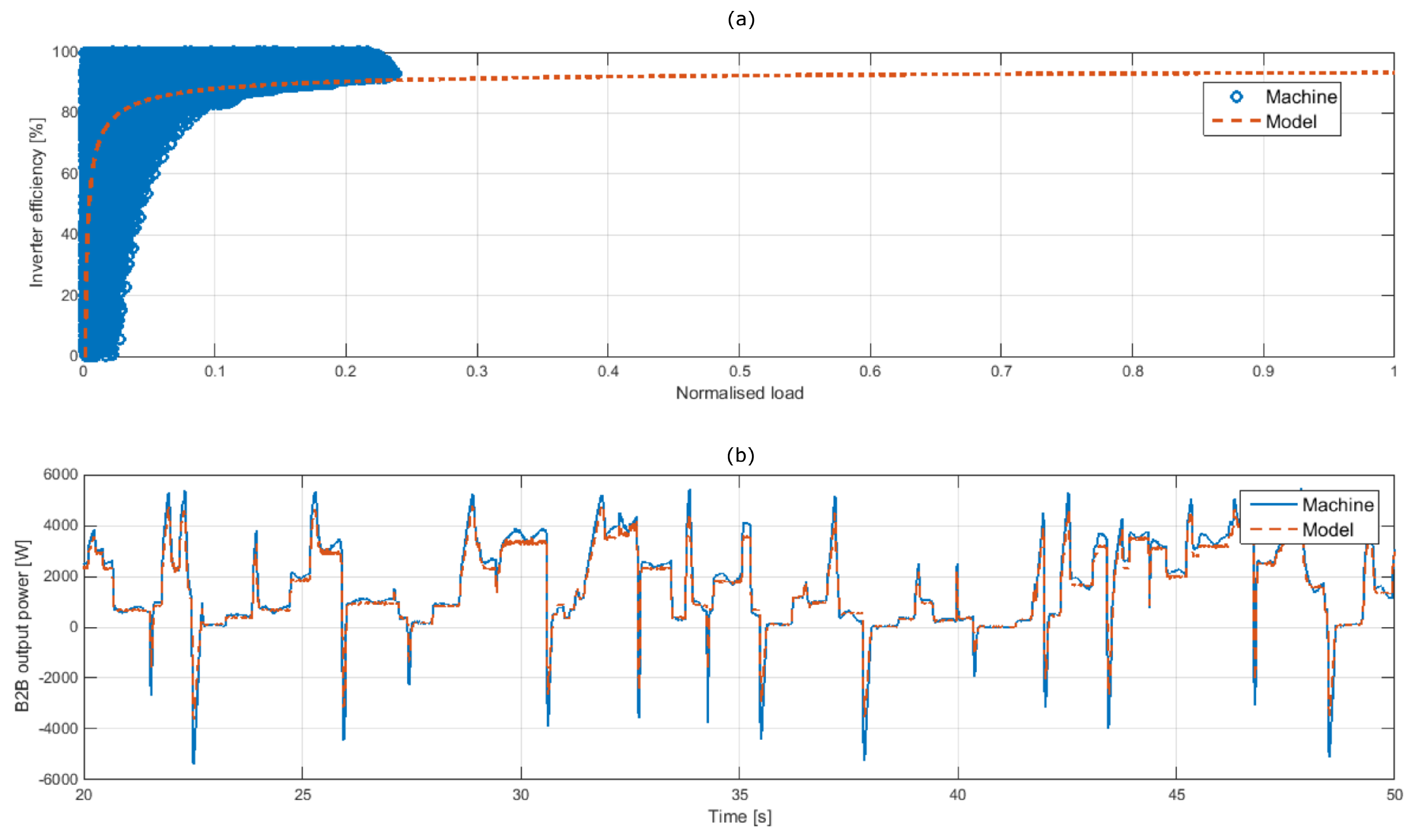
Therefore, another alternative to evaluate power losses in the power converters is suggested in this paper. Power measurements at the input and output of the B2B power converter are available in the experiments, from where the power losses in the B2B converter can be extracted.
Inverters’ efficiency varies as a function of load, with considerable efficiency drops at part-load and overload conditions [45]. However, measurements in the experiments only cover the part-load operation of the inverters, since the rated power of the DFIG is lower than the rated power of the inverters used in the B2B converter (see Table A3 and Table A4 in the Appendix A).
Figure 17a shows the efficiency of one inverter in the B2B converter as a function of normalised load, defined as the ratio between the input power of the B2B converter and the rated power of the inverters. The points from the experimental measurements clearly show the trend of the efficiency curve, so a power trend line, described in Equation (25), is used to fit the experimental measurements, as shown in Figure 17a. Using the fitted curve, power losses in the inverters can be calculated without prohibitively increasing the computational requirements of the mathematical model. Table 5 shows the fidelity values of the power losses in the inverters of the B2B converter, obtained by comparing losses measured in the experimental platform to the losses obtained in the mathematical model, and Figure 17b illustrates the power output of the B2B converter for the machine and the model. Fidelity values for all of the test cases show good agreement, particularly good for the test case Test 1c. This is because the efficiency curve is fitted using the specific data from Test 1c.
6. Conclusions
Mathematical models for three different electric generators (squirrel-cage induction generator, permanent magnet synchronous generator and doubly-fed induction generator) are validated in the present paper against experimental data from three real machines. In addition, the model for a back-to-back power converter is validated in this paper, using the data generated from the experiments in the doubly-fed induction generator connected to the grid in a back-to-back configuration. The mathematical models for the three electric generators and the back-to-back power converter are given in Section 2.
The experimental platform to generate the experimental data is described in Section 3. The validation is carried out comparing results from the mathematical models and the experiments by means of fidelity values based on the moving average normalised root mean square error. Six different test cases are designed for the validation, three of which are based on random signals generated using random-amplitude random-phase sequences, and the other three are based on realistic PTO signals generated using a W2W model with a hydraulic transmissions system, as shown in Section 4. That way, the whole operation range of the electric generators is covered.
The mathematical model of the B2B power converter, presented in Section 2.3, neglects the harmonics generated by the PWM due to the extremely low time step required to accurately model the operations of power switches in the inverters, which prohibitively increases the computational requirements of the mathematical models. Hence, in the mathematical models, voltage signals delivered from the inverters into the electric generator and electricity grid only include the fundamental frequency determined in the controller. Therefore, the present paper suggests using an efficiency curve for inverters to include power losses without increasing computational requirements. Such an efficiency curve is determined by using a power trend line fitted to experimental data, as described in Section 5.2.
Overall, the fidelity values for the three electric generators and the back-to-back power converter, presented in Section 5.1 and Section 5.2, respectively, show very satisfactory agreement between the results obtained from the experimental platforms and the mathematical models. Therefore, this paper demonstrates the suitability of the mathematical models described in Section 2.1 and Section 2.2, in spite of the neglected iron losses in the generator and the harmonics generated by the PWM.
Acknowledgments
This material is based on works supported by the Science Foundation Ireland under Grant No. 13/IA/1886.
Author Contributions
Markel Penalba and John V. Ringwood participated in implementing the mathematical models, while José-Antonio Cortajarena designed and constructed the experimental platforms and ran the simulations in those platforms. Markel Penalba wrote the manuscript, and José-Antonio Cortajarena and John V. Ringwood revised it critically for important intellectual content. Finally, all authors gave the final approval of the version to be submitted and any revised version.
Conflicts of Interest
The authors declare no conflict of interest.
Appendix A. Experimental Platform Parameters
Appendix A.1. Machine Parameters
The parameters of the three machines are given in the following Table A1, Table A2 and Table A3 for the SCIG, the PMSG and the DFIG, respectively.

Table A1.
Ratings and parameters of the SCIG.
| Nominal power | 7500 W |
| Stator voltage | 380 V |
| Rated stator current | 21 A |
| Rated speed | 1450 rpm @ 50 Hz |
| Rated torque | 50 Nm |
| Stator resistance | 0.729 |
| Rotor resistance | 0.40 |
| Magnetizing inductance | 0.111 H |
| Stator leakage inductance | 0.1152 H |
| Rotor leakage inductance | 0.1138 H |
| Inertia moment | 0.045 kg·m |
| Friction/windage damping | 0.015 N·m·s |
Table A2.
Rating and parameters of the PMSG.
| Nominal power | 3830 W |
| Stator voltage | 380 V |
| Rated stator current | 15 A |
| Rated speed | 3000 rpm @ 50 Hz |
| Rated torque | 12.2 Nm |
| Stator resistance | 0.49 |
| Stator (d-axis) leakage inductance | 0.0069 H |
| Stator (q-axis) leakage inductance | 0.039 H |
| Rotor permanent magnet flux | 0.2484 Wb |
| Inertia moment | 0.006 kg·m |
| Friction/windage damping | 0.008 N·m·s |
Table A3.
Ratings and parameters of the DFIG.
| Nominal power | 7500 W |
| Stator voltage | 380 V |
| Rated stator current | 18 A |
| Rated rotor current | 24 A |
| Rated speed | 1447 rpm @ 50 Hz |
| Rated torque | 50 Nm |
| Stator resistance | 0.42 |
| Rotor resistance | 0.70 |
| Magnetizing inductance | 0.055 H |
| Stator leakage inductance | 0.06 H |
| Rotor leakage inductance | 0.06 H |
| Inertia moment | 0.04 kg·m |
| Friction/windage damping | 0.001 N·m·s |
Appendix A.2. Power Converter Parameters
The characteristics of the power converter units used in the experimental platform are given in Table A4.
Table A4.
Rating of the power converter units.
| Nominal power | 35 kW |
| Switching frequency | 7 kHz |
| Inverter gain | 310 |
| Dead-time | 1.4 s |
References
- Antonio, F.D.O. Wave energy utilization: A review of the technologies. Renew. Sustain. Energy Rev. 2010, 14, 899–918. [Google Scholar]
- Viviano, A.; Naty, S.; Foti, E.; Bruce, T.; Allsop, W.; Vicinanza, D. Large-scale experiments on the behaviour of a generalised Oscillating Water Column under random waves. Renew. Energy 2016, 99, 875–887. [Google Scholar] [CrossRef]
- Whittaker, T.; Collier, D.; Folley, M.; Osterried, M.; Henry, A.; Crowley, M. The development of Oyster—A shallow water surging wave energy converter. In Proceedings of the 7th European Wave and Tidal Energy Conference, Porto, Portugal, 1–14 September 2007. [Google Scholar]
- Hals, J.; Ásgeirsson, S.G.; Hjálmarsson, E.; Maillet, J.; Moller, P.; Pires, P.; Guérinel, M.; Lopes, M. Tank testing of an inherently phase-controlled wave energy converter. Int. J. Mar. Energy 2016, 15, 68–84. [Google Scholar]
- Iuppa, C.; Contestabile, P.; Cavallaro, L.; Foti, E.; Vicinanza, D. Hydraulic performance of an innovative breakwater for overtopping wave energy conversion. Sustainability 2016, 8, 1226. [Google Scholar] [CrossRef]
- Ringwood, J.V.; Bacelli, G.; Fusco, F. Control, forecasting and optimisation for wave energy conversion. IFAC Proc. Vol. 2014, 47, 7678–7689. [Google Scholar] [CrossRef]
- Cretel, J.; Lewis, A.; Lightbody, G.; Thomas, G. An application of model predictive control to a wave energy point absorber. IFAC Proc. Vol. 2010, 43, 267–272. [Google Scholar] [CrossRef]
- Bacelli, G.; Ringwood, J.V. Numerical optimal control of wave energy converters. IEEE Trans. Sustain. Energy 2015, 6, 294–302. [Google Scholar] [CrossRef]
- Hals, J.; Falnes, J.; Moan, T. Constrained optimal control of a heaving buoy wave-energy converter. J. Offshore Mech. Arct. Eng. 2011, 133, 011401. [Google Scholar] [CrossRef]
- Genest, R.; Ringwood, J.V. Receding horizon pseudospectral control for energy maximization with application to wave energy devices. IEEE Trans. Control Syst. Technol. 2017, 25, 29–38. [Google Scholar] [CrossRef]
- Penalba, M.; Ringwood, J.V. A Review of Wave-to-Wire Models for Wave Energy Converters. Energies 2016, 9, 506. [Google Scholar] [CrossRef]
- Bailey, H.; Robertson, B.R.; Buckham, B.J. Wave-to-wire simulation of a floating oscillating water column wave energy converter. Ocean Eng. 2016, 125, 248–260. [Google Scholar] [CrossRef]
- Garcia-Rosa, P.B.; Vilela Soares Cunha, J.P.; Lizarralde, F.; Estefen, S.F.; Machado, I.R.; Watanabe, E.H. Wave-to-Wire Model and Energy Storage Analysis of an Ocean Wave Energy Hyperbaric Converter. IEEE J. Ocean. Eng. 2014, 39, 386–397. [Google Scholar] [CrossRef]
- Tedeschi, E.; Carraro, M.; Molinas, M.; Mattavelli, P. Effect of Control Strategies and Power Take-Off Efficiency on the Power Capture From Sea Waves. IEEE Trans. Energy Convers. 2011, 26, 1088–1098. [Google Scholar] [CrossRef]
- Amundarain, M.; Alberdi, M.; Garrido, A.J.; Garrido, I. Modeling and Simulation of Wave Energy Generation Plants: Output Power Control. IEEE Trans. Ind. Electron. 2011, 58, 105–117. [Google Scholar] [CrossRef]
- Gear, C.W.; Wells, D. Multirate linear multistep methods. BIT Numer. Math. 1984, 24, 484–502. [Google Scholar] [CrossRef]
- Engstler, C.; Lubich, C. Multirate extrapolation methods for differential equations with different time scales. Computing 1997, 58, 173–185. [Google Scholar] [CrossRef]
- Giorgi, G.; Penalba, M.; Ringwood, J.V. Nonlinear Hydrodynamic Models for Heaving Buoy Wave Energy Converters. In Proceedings of the 3rd Asian Wave and Tidal Energy Conference, Singapore, 24–28 October 2016; pp. 144–153. [Google Scholar]
- Penalba, M.; Sell, N.P.; Hillis, A.J.; Ringwood, J.V. Validating a Wave-to-Wire Model for a Wave Energy Converter—Part I: The Hydraulic Transmission System. Energ. 2017, 10, 977. [Google Scholar] [CrossRef]
- Wu, F.; Zhang, X.P.; Ju, P.; Sterling, M.J. Modeling and Control of AWS-Based Wave Energy Conversion System Integrated Into Power Grid. IEEE Trans. Power Syst. 2008, 23, 1196–1204. [Google Scholar]
- O’Sullivan, A.C.; Lightbody, G. Co-design of a wave energy converter using constrained predictive control. Renew. Energy 2017, 102, 142–156. [Google Scholar] [CrossRef]
- Hansen, R.H.; Kramer, M.M.; Vidal, E. Discrete displacement hydraulic power take-off system for the wavestar wave energy converter. Energies 2013, 6, 4001–4044. [Google Scholar] [CrossRef]
- Sjolte, J.; Tjensvoll, G.; Molinas, M. Power collection from wave energy farms. Appl. Sci. 2013, 3, 420–436. [Google Scholar] [CrossRef]
- Danielsson, O. Wave Energy Conversion: Linear Synchronous Permanent Magnet Generator. Ph.D. Thesis, Acta Universitatis Upsaliensis, Uppsala, Sweden, 2006. [Google Scholar]
- Cruz, J. Ocean Wave Energy: Current Status and Future Perspectives; Springer: Berlin/Heidelberg, Germany, 2008. [Google Scholar]
- Park, R.H. Two-reaction theory of synchronous machines generalized method of analysis—Part I. Trans. American Inst. Electr. Eng. 1929, 48, 716–727. [Google Scholar] [CrossRef]
- Mohan, N. Advanced Electric Drives: Analysis, Control, and Modeling Using MATLAB/Simulink; John Wiley & Sons: Hoboken, NJ, USA, 2014. [Google Scholar]
- Krause, P.C.; Wasynczuk, O.; Sudhoff, S.D.; Pekarek, S. Analysis of Electric Machinery and Drive Systems, 3rd ed.; IEEE Press Series on Power Engineering; Wiley-Blackwell: Piscataway, NJ, USA, 2013. [Google Scholar]
- Prasad, M.; Gayen, P.K.; Chatterjee, D. A harmonic elimination technique for voltage source inverter using embedded controller. In Proceedings of the 2016 International Conference on Microelectronics, Computing and Communications (MicroCom), Durgapur, India, 23–25 January 2016; pp. 1–6. [Google Scholar]
- Pena, R.; Clare, J.; Asher, G. Doubly fed induction generator using back-to-back PWM converters and its application to variable-speed wind-energy generation. IEE Proc Electr. Power Appl. 1996, 143, 231–241. [Google Scholar] [CrossRef]
- Bai, H.; Wang, F.; Xing, J. Control strategy of combined PWM rectifier/inverter for a high speed generator power system. In Proceedings of the 2007 2nd IEEE Conference on Industrial Electronics and Applications, Harbin, China, 23–25 May 2007; pp. 132–135. [Google Scholar]
- Tamura, J. Calculation method of losses and efficiency of wind generators. In Wind Energy Conversion System; Springer: Berlin/Heidelberg, Germany, 2012; pp. 25–51. [Google Scholar]
- Barambones, O.; Cortajarena, J.A.; Alkorta, P.; de Durana, J.M.G. A real-time sliding mode control for a wind energy system based on a doubly fed induction generator. Energies 2014, 7, 6412–6433. [Google Scholar] [CrossRef]
- Cortajarena, J.A.; De Marcos, J. Neural network model reference adaptive system speed estimation for sensorless control of a doubly fed induction generator. Electr. Power Compon. Syst. 2013, 41, 1146–1158. [Google Scholar] [CrossRef]
- Ljung, L. System Identification: Theory for the User; Prentice Hall PTR: Upper Saddle River, NJ, USA, 1999. [Google Scholar]
- Pintelon, R.; Schoukens, J. System Identification: A Frequency Domain Approach; John Wiley & Sons: Hoboken, NJ, USA, 2012. [Google Scholar]
- Ringwood, J.V.; Davidson, J.; Giorgi, S. Model Identification from recorded WEC data. In Numerical Modelling of Wave Energy Converters: State-of-the-Art Techniques for Single Devices and Arrays; Folley, M., Ed.; Elsevier: London, UK, 2016; pp. 123–148. [Google Scholar]
- Igic, P.; Zhou, Z.; Knapp, W.; MacEnri, J.; Sørensen, H.; Friis-Madsen, E. Multi-megawatt offshore wave energy converters–electrical system configuration and generator control strategy. IET Renew. Power Gener. 2011, 5, 10–17. [Google Scholar] [CrossRef]
- Cargo, C.J.; Hillis, A.J.; Plummer, A.R. Optimisation and control of a hydraulic power take-off unit for a wave energy converter in irregular waves. Proc. Inst. Mech. Eng. Part A J. Power Energy 2014, 228, 462–479. [Google Scholar] [CrossRef]
- Ramirez, D.; Bartolome, J.P.; Martinez, S.; Herrero, L.C.; Blanco, M. Emulation of an OWC ocean energy plant with PMSG and irregular wave model. IEEE Trans. Sustain. Energy 2015, 6, 1515–1523. [Google Scholar] [CrossRef]
- Hansen, R.H.; Andersen, T.O.; Pedersen, H.C. Model based design of efficient power take-off systems for wave energy converters. In Proceedings of the 12th Scandinavian International Conference on Fluid Power, Tampere, Finland, 18–20 May 2011. [Google Scholar]
- Hasselmann, K.; Barnett, T.; Bouws, E.; Carlson, H.; Cartwright, D.; Enke, K.; Ewing, J.; Gienapp, H.; Hasselmann, D.; Kruseman, P.; et al. Measurements of Wind-Wave Growth and Swell Decay During the Joint North Sea Wave Project (JONSWAP); Technical Report; Deutsches Hydrographisches Institut: Hamburg, Germany, 1973. [Google Scholar]
- Plummer, A.; Cargo, C.C. Power Transmissions for Wave Energy Converters: A Review. In Proceedings of the 8th International Fluid Power Conference (IFK), Dresden, Germany, 26–28 March 2012. [Google Scholar]
- Rabinovich, S.G. Measurement Errors and Uncertainties: Theory and Practice; Springer: Basking Ridge, NJ, USA, 2006. [Google Scholar]
- Mondol, J. Sizing of grid-connected photovoltaic systems. SPIE 2007, 1–3. [Google Scholar]
Figure 1.
Full conversion chain of a wave energy converter with hydraulic power take-off (PTO); adapted from [11].
Figure 1.
Full conversion chain of a wave energy converter with hydraulic power take-off (PTO); adapted from [11].
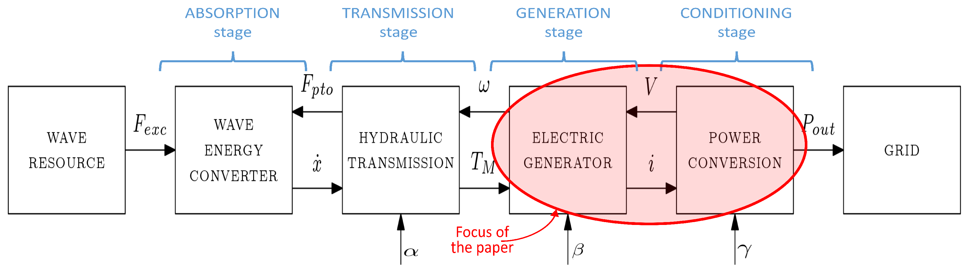
Figure 2.
Induction generator dq equivalent circuit, based on [27], where (a) represents the d-axis and (b) represents the q-axis.
Figure 2.
Induction generator dq equivalent circuit, based on [27], where (a) represents the d-axis and (b) represents the q-axis.
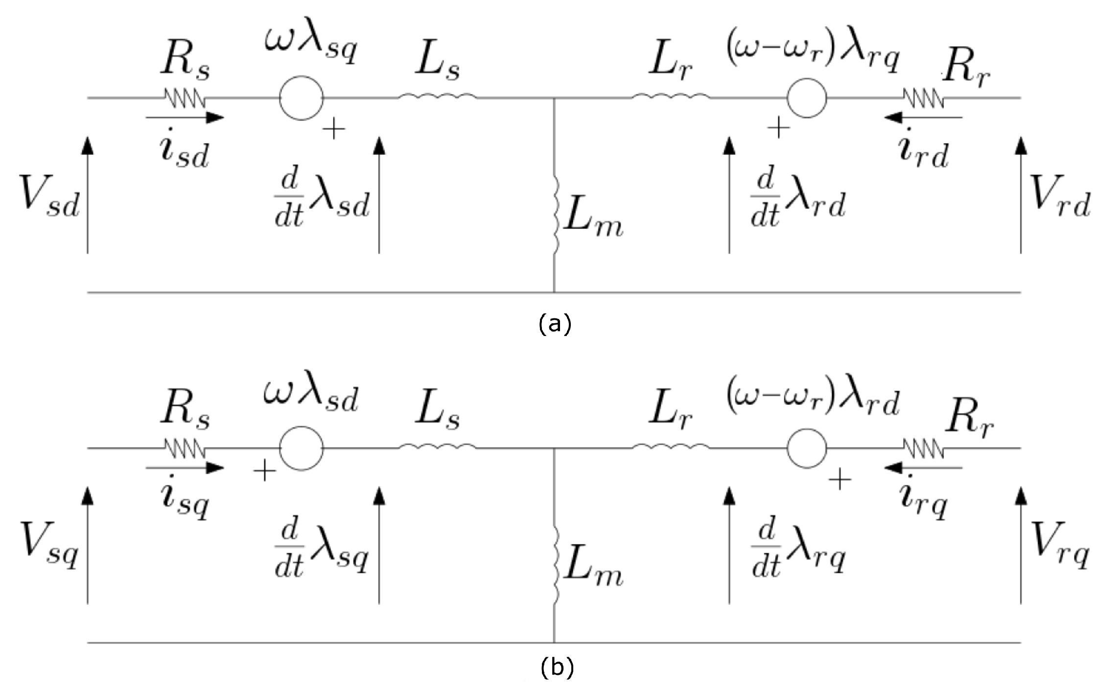
Figure 3.
Permanent magnet synchronous generator (PMSG) dq equivalent circuit, based on [27], where (a) represents the d-axis and (b) represents the q-axis.
Figure 3.
Permanent magnet synchronous generator (PMSG) dq equivalent circuit, based on [27], where (a) represents the d-axis and (b) represents the q-axis.
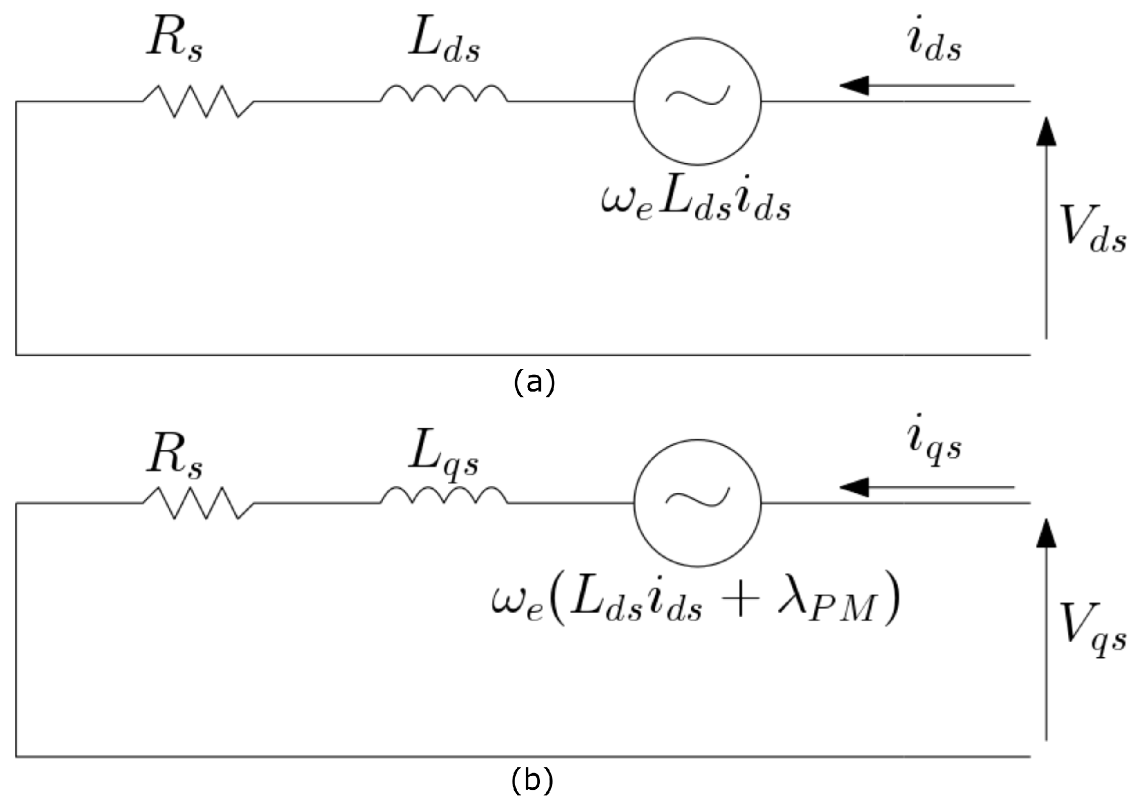
Figure 4.
Diagram of a back-to-back power converter with controllers and pulse width modulators. GenSI, generator-side inverter.
Figure 4.
Diagram of a back-to-back power converter with controllers and pulse width modulators. GenSI, generator-side inverter.
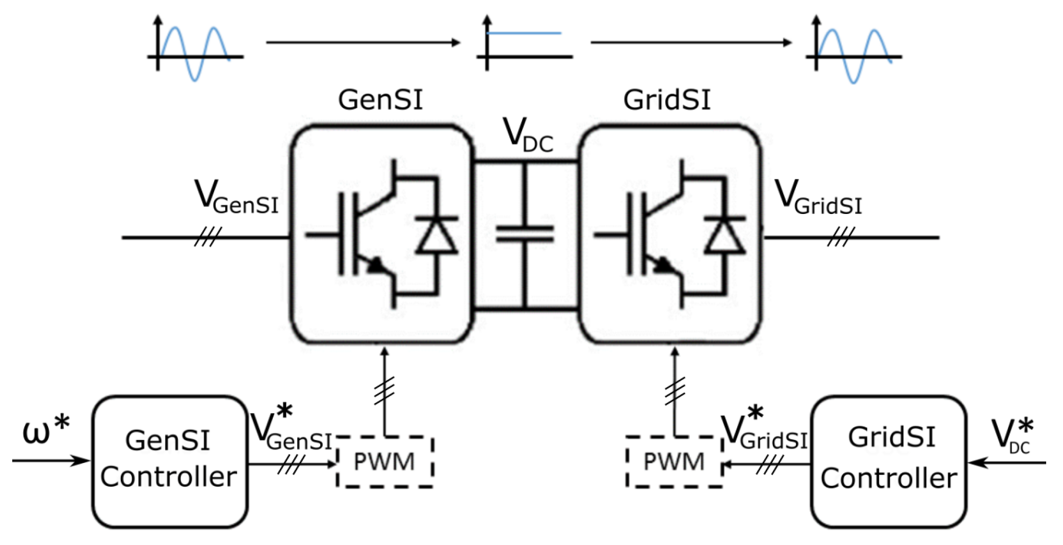
Figure 5.
Specific power losses in an electric generator.
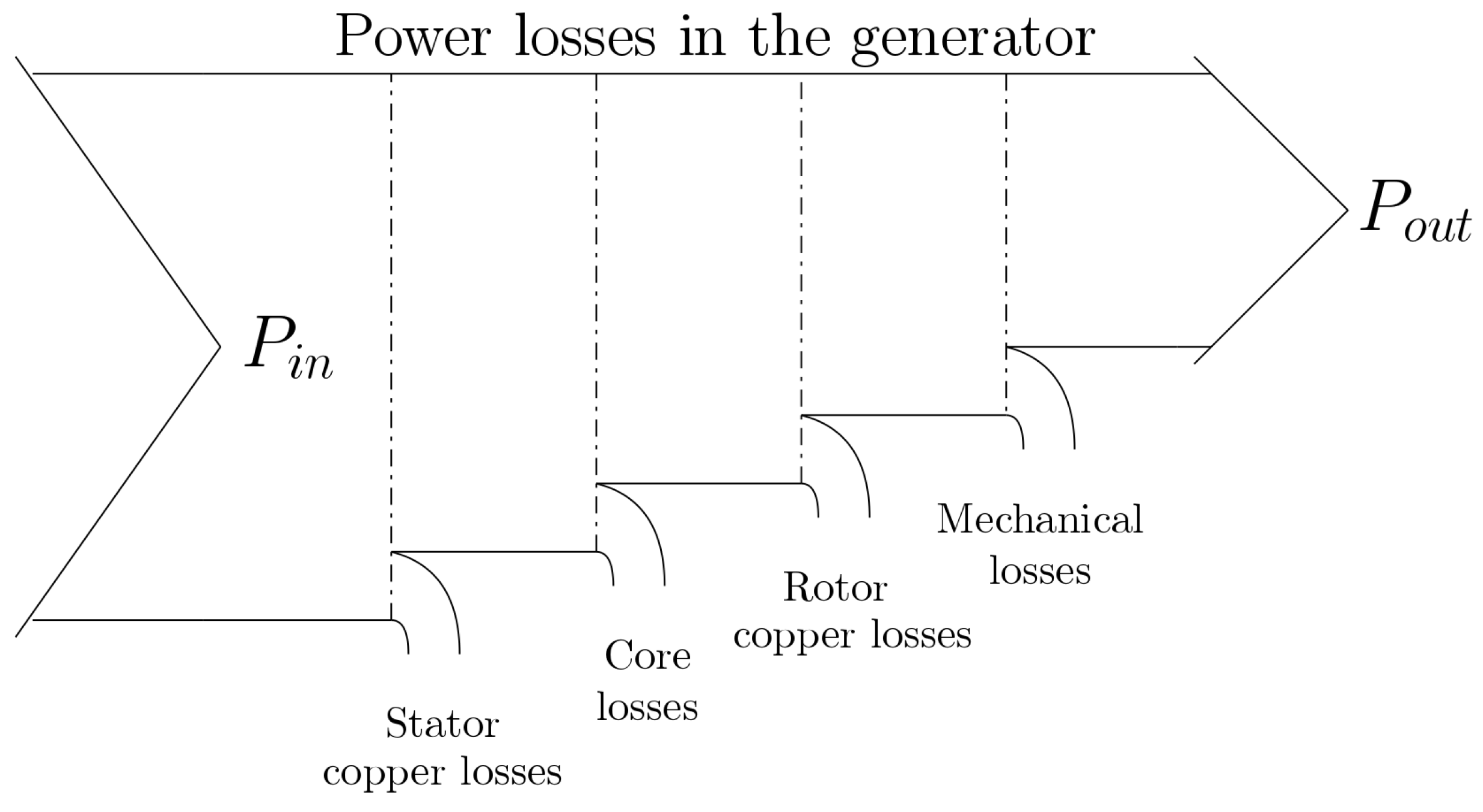
Figure 6.
Diagram of a typical switching operation of a power switch that illustrates the (non-ideal) switching and conduction phases and the power losses related to each phase.
Figure 6.
Diagram of a typical switching operation of a power switch that illustrates the (non-ideal) switching and conduction phases and the power losses related to each phase.
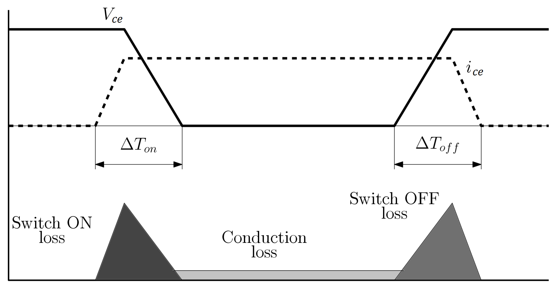
Figure 7.
Diagram of the experimental platform for the doubly-fed induction generator (DFIG) [33]; see the text for the squirrel-cage induction generator (SCIG) and PMSG experimental configurations.
Figure 7.
Diagram of the experimental platform for the doubly-fed induction generator (DFIG) [33]; see the text for the squirrel-cage induction generator (SCIG) and PMSG experimental configurations.

Figure 8.
Picture of the experimental platform [33].
Figure 8.
Picture of the experimental platform [33].
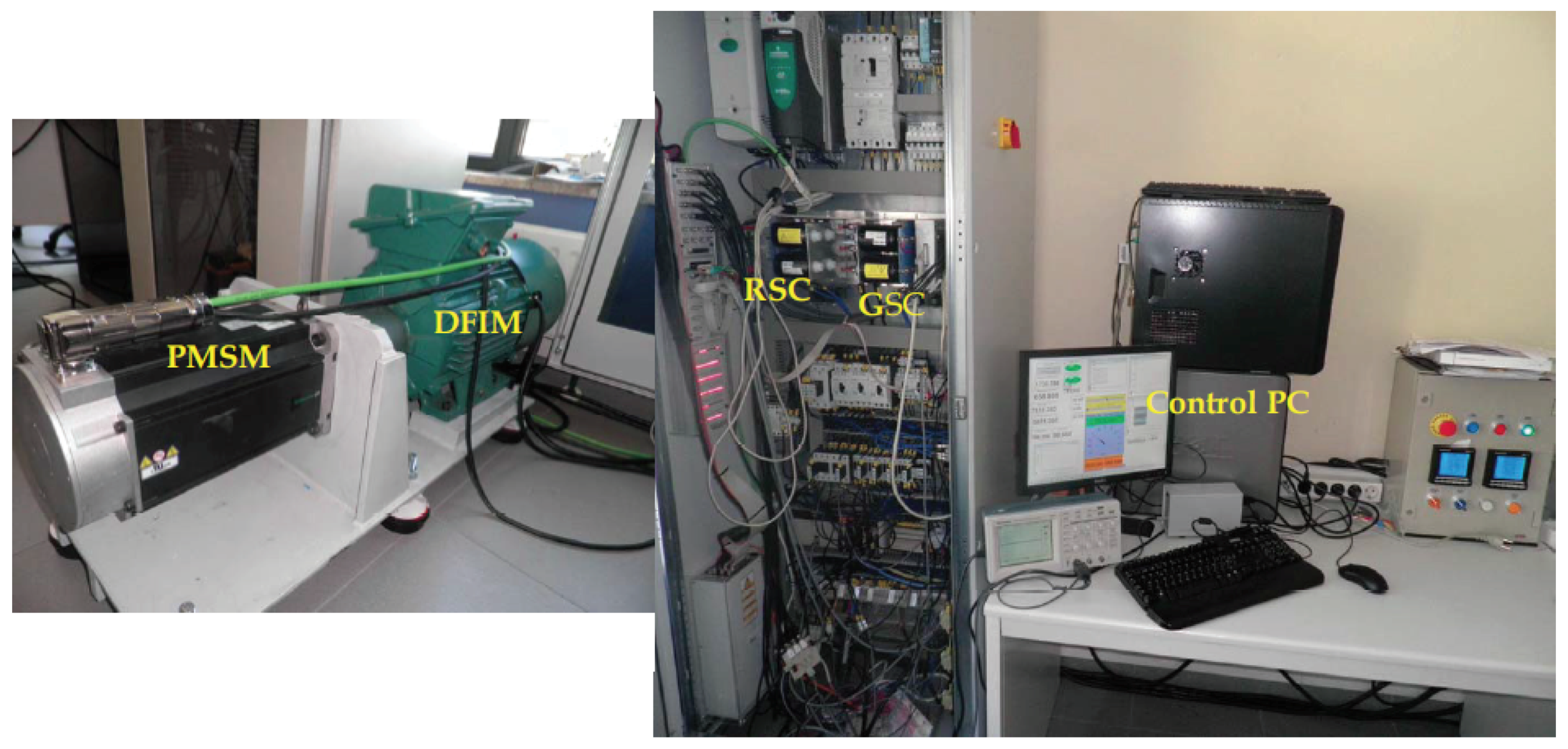
Figure 9.
Diagram of the electric generator validation system, including the generator-side inverter and the controller, showing the inputs and the outputs.
Figure 9.
Diagram of the electric generator validation system, including the generator-side inverter and the controller, showing the inputs and the outputs.

Figure 10.
The random-amplitude random-phase (RARP) signals for the reference rotational speed and torque (a) and their spectral (b) and amplitude (c) properties.
Figure 10.
The random-amplitude random-phase (RARP) signals for the reference rotational speed and torque (a) and their spectral (b) and amplitude (c) properties.
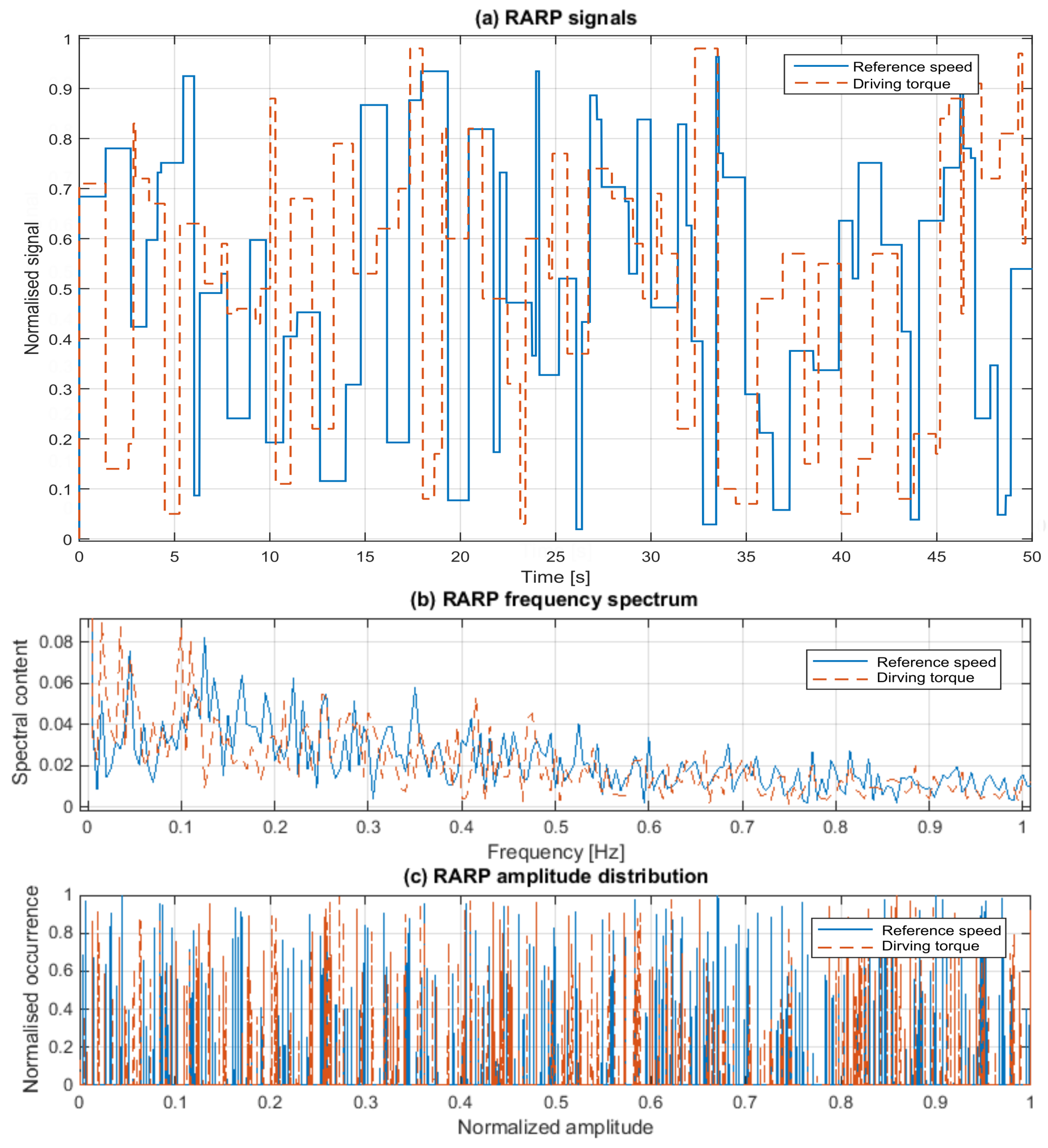
Figure 11.
The three signals based on realistic PTO systems: constant torque and rotational speed (a), variable torque and constant rotational speed (b) and variable torque and rotational speed (c).
Figure 11.
The three signals based on realistic PTO systems: constant torque and rotational speed (a), variable torque and constant rotational speed (b) and variable torque and rotational speed (c).
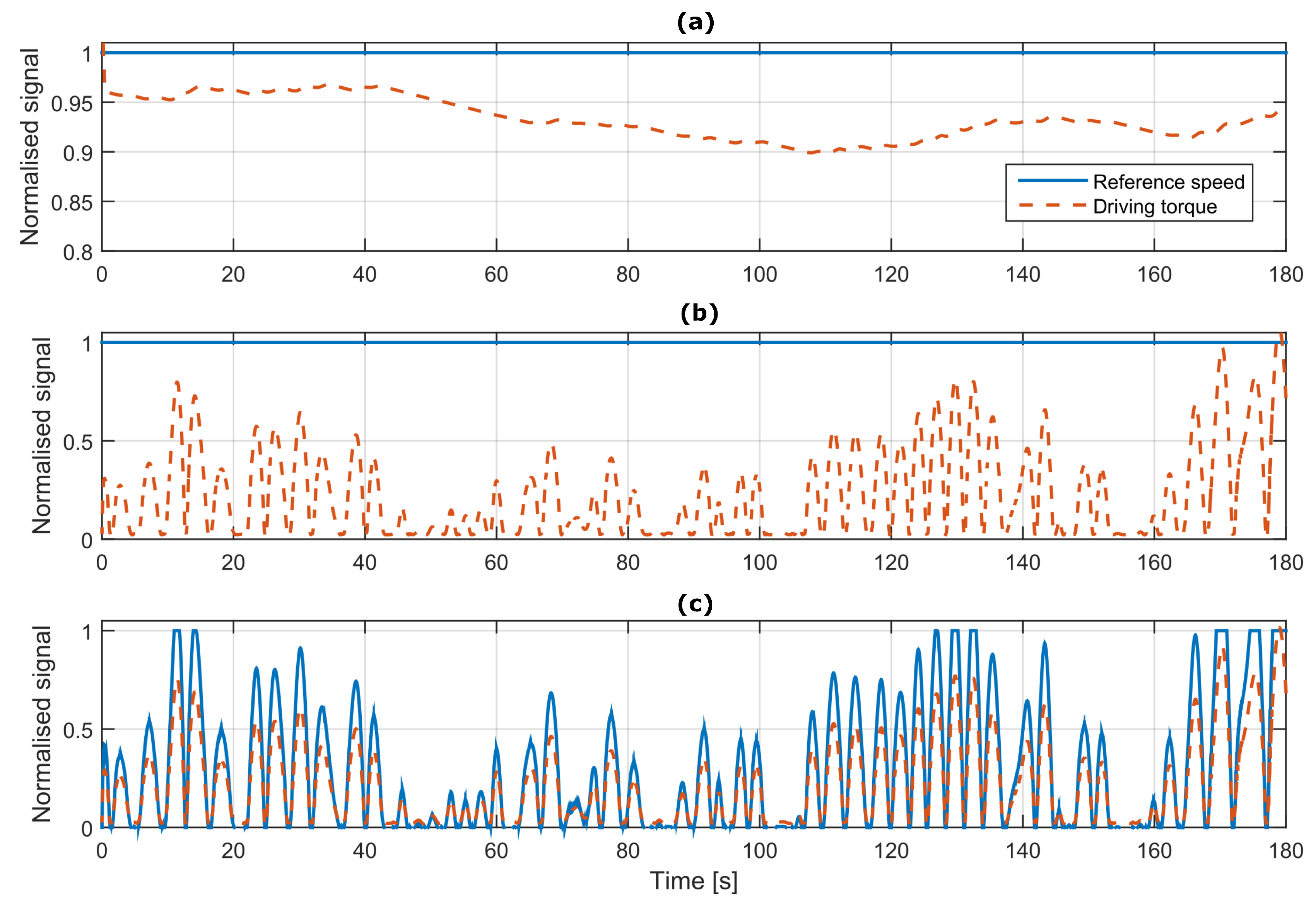
Figure 12.
Comparing results from experiments and numerical models for the SCIG: rotational speed for Test 1a (a), real power for Test 1c (b), electromagnetic torque for Test 2b (c) and reactive power for Test 2c (d).
Figure 12.
Comparing results from experiments and numerical models for the SCIG: rotational speed for Test 1a (a), real power for Test 1c (b), electromagnetic torque for Test 2b (c) and reactive power for Test 2c (d).
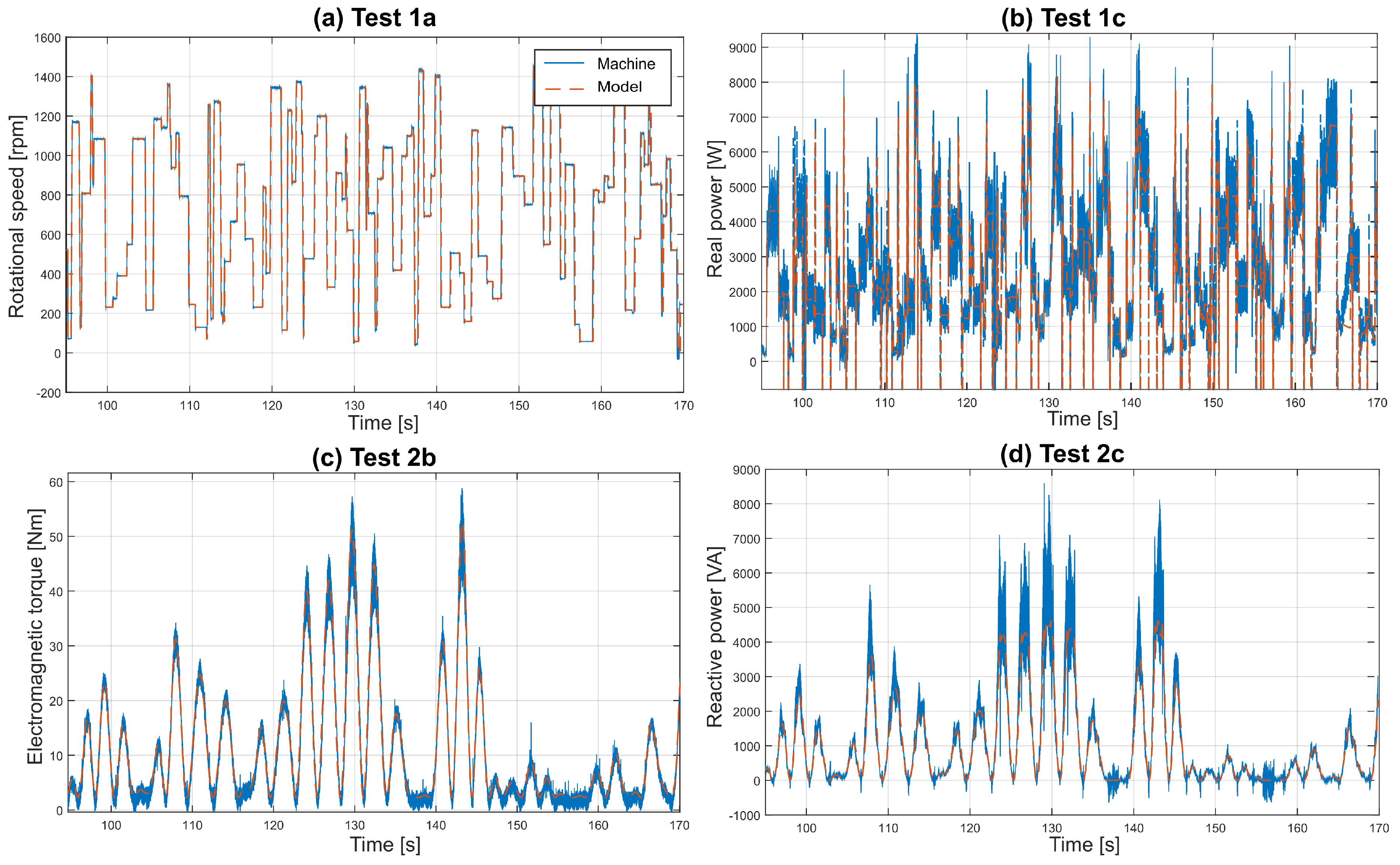
Figure 13.
Frequency content of the stator voltage signals in Test2b from machine measurements and models results.
Figure 13.
Frequency content of the stator voltage signals in Test2b from machine measurements and models results.

Figure 14.
Real power measurements in the SCIG and the PMSG for the Test 2c test case: power values (a) and normalised power showing the noise level (b).
Figure 14.
Real power measurements in the SCIG and the PMSG for the Test 2c test case: power values (a) and normalised power showing the noise level (b).

Figure 15.
Efficiency of the SCIG (a); PMSG (b) and DFIG (c) for the Test 1c test case.
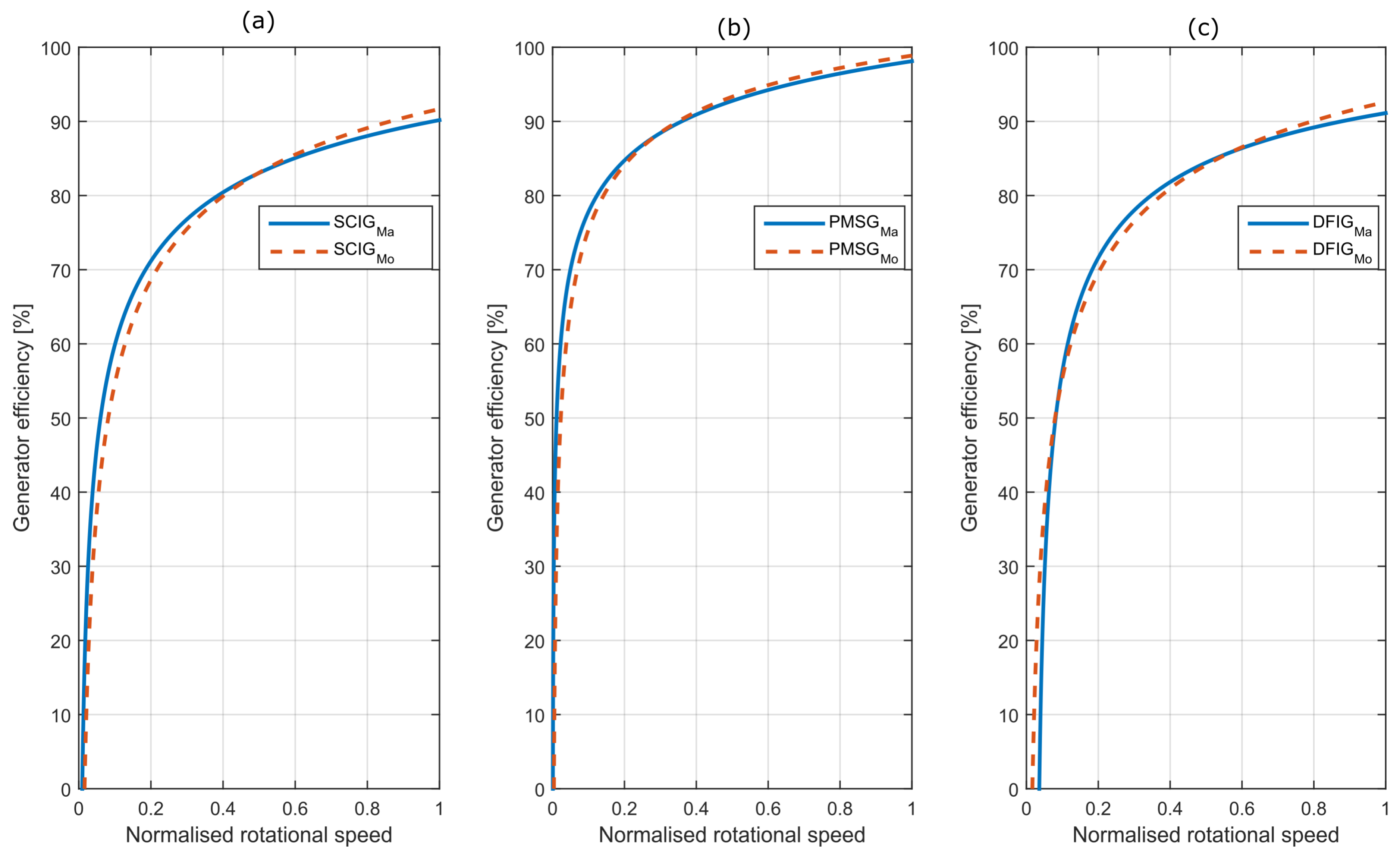
Figure 16.
The efficacy of the control implemented in the GenSI and GridSI in the mathematical model compared to the measures of the real machine: power in the stator (a) and DC-link voltage (b).
Figure 16.
The efficacy of the control implemented in the GenSI and GridSI in the mathematical model compared to the measures of the real machine: power in the stator (a) and DC-link voltage (b).

Figure 17.
Inverter efficiency as a function of normalised load (a), including the fitted curve, and power output of the B2B power converter for the machine and the model (b).
Figure 17.
Inverter efficiency as a function of normalised load (a), including the fitted curve, and power output of the B2B power converter for the machine and the model (b).

Table 1.
Fidelity measures for the SCIG.
| Test 1a | Test 1b | Test 1c | Test 2a | Test 2b | Test 2c | |
|---|---|---|---|---|---|---|
| 98.64 | 98.09 | 98.68 | 89.92 | 98.53 | 99.61 | |
| 93.33 | 97.72 | 94.26 | 86.47 | 97.05 | 94.03 | |
| 96.43 | 95.22 | 95.33 | 82.15 | 95.57 | 94.42 | |
| 97.25 | 93.78 | 96.13 | 81.03 | 92.70 | 93.80 | |
| 96.72 | 90.71 | 94.60 | 78.87 | 86.52 | 95.13 | |
| 97.01 | 96.25 | 91.87 | 79.98 | 85.74 | 92.49 |
Table 2.
Fidelity measures for the PMSG.
| Test 1a | Test 1b | Test 1c | Test 2a | Test 2b | Test 2c | |
|---|---|---|---|---|---|---|
| 97.03 | 95.51 | 97.19 | 88.90 | 97.06 | 98.70 | |
| 94.55 | 94.69 | 94.59 | 81.84 | 90.29 | 93.98 | |
| 93.58 | 93.13 | 94.31 | 72.72 | 92.20 | 92.14 | |
| 94.66 | 91.34 | 95.02 | 77.45 | 87.28 | 94.95 | |
| 93.34 | 92.49 | 93.87 | 78.56 | 85.77 | 88.43 | |
| 92.59 | 91.00 | 94.50 | 75.35 | 84.39 | 87.85 |
Table 3.
Fidelity measures for the DFIG.
| Test 1a | Test 1b | Test 1c | Test 2a | Test 2b | Test 2c | |
|---|---|---|---|---|---|---|
| 99.08 | 98.49 | 99.05 | 91.46 | 97.86 | 98.06 | |
| 93.57 | 96.72 | 95.26 | 83.07 | 91.75 | 94.72 | |
| 96.34 | 95.22 | 95.63 | 76.34 | 92.36 | 91.47 | |
| 95.34 | 94.78 | 94.78 | 77.13 | 88.41 | 94.73 | |
| 93.72 | 91.26 | 94.21 | 79.91 | 86.97 | 89.66 | |
| 95.70 | 96.47 | 91.38 | 76.38 | 84.67 | 88.47 |
Table 4.
Coefficients of the power function used to fit the trend line of the real machines.
| SCIGMa | SCIGMa | PMSGMa | PMSGMa | DFIGMa | DFIGMa | |
|---|---|---|---|---|---|---|
| −264.1 | −335.4 | −164 | −245.4 | −20.88 | −34.58 | |
| −0.2868 | −0.3017 | −0.1591 | −0.2817 | −0.3802 | −0.3175 | |
| 122.6 | 128.6 | 144 | 124.6 | 110.2 | 127.2 |
Table 5.
Fidelity measures for the back-to-back (B2B) converter.
| Test 1a | Test 1b | Test 1c | Test 2a | Test 2b | Test 2c | |
|---|---|---|---|---|---|---|
| 96.39 | 96.72 | 95.81 | 96.37 | 97.13 | 96.78 | |
| 94.61 | 95.27 | 98.47 | 87.43 | 95.71 | 94.86 |
© 2017 by the authors. Licensee MDPI, Basel, Switzerland. This article is an open access article distributed under the terms and conditions of the Creative Commons Attribution (CC BY) license (http://creativecommons.org/licenses/by/4.0/).
Share and Cite
MDPI and ACS Style
Penalba, M.; Cortajarena, J.-A.; Ringwood, J.V. Validating a Wave-to-Wire Model for a Wave Energy Converter—Part II: The Electrical System. Energies 2017, 10, 1002. https://doi.org/10.3390/en10071002
AMA Style
Penalba M, Cortajarena J-A, Ringwood JV. Validating a Wave-to-Wire Model for a Wave Energy Converter—Part II: The Electrical System. Energies. 2017; 10(7):1002. https://doi.org/10.3390/en10071002
Chicago/Turabian StylePenalba, Markel, José-Antonio Cortajarena, and John V. Ringwood. 2017. "Validating a Wave-to-Wire Model for a Wave Energy Converter—Part II: The Electrical System" Energies 10, no. 7: 1002. https://doi.org/10.3390/en10071002
Note that from the first issue of 2016, this journal uses article numbers instead of page numbers. See further details here.