
A Novel Decentralized Economic Operation in Islanded AC Microgrids


1
School of Information Science and Engineering, Central South University, Changsha 410083, China
2
School of Automation Science and Electrical Engineering, Beihang University, Beijing 100191, China
3
Department of Electrical Engineering, University of Arkansas, Fayetteville, AR 72701, USA
4
Department of Energy Technology, Aalborg University, DK-9220 Aalborg East, Denmark
*
Author to whom correspondence should be addressed.
Energies 2017, 10(6), 804; https://doi.org/10.3390/en10060804
Submission received: 16 April 2017
/
Revised: 27 May 2017
/
Accepted: 9 June 2017
/
Published: 13 June 2017
(This article belongs to the Special Issue Advanced Operation and Control of Smart Microgrids)
Abstract
:Droop schemes are usually applied to the control of distributed generators (DGs) in microgrids (MGs) to realize proportional power sharing. The objective might, however, not suit MGs well for economic reasons. Addressing that issue, this paper proposes an alternative droop scheme for reducing the total active generation costs (TAGC). Optimal economic operation, DGs’ capacity limitations and system stability are fully considered basing on DGs’ generation costs. The proposed scheme utilizes the frequency as a carrier to realize the decentralized economic operation of MGs without communication links. Moreover, a fitting method is applied to balance DGs’ synchronous operation and economy. The effectiveness and performance of the proposed scheme are verified through simulations and experiments.
1. Introduction
Recently, interest has been concentrated on microgrids (MGs) [1,2,3,4], which represent an effective approach to deal with distributed generation [5,6,7,8]. Usually, a MG comprises different types of distributed generators (DGs), such as diesel generators, wind turbines, photovoltaic (PV) generators, energy storage units, etc. Different DGs have different generation costs [9,10,11]. From the economical perspective, less costly DGs should be controlled to provide more power and all DGs in the MGs should be coordinated in economic operation modes [12,13,14].
The economical control approaches in MGs can be classified into the centralized, distributed and decentralized schemes. The centralized control in a hierarchical coordination control manner is proposed in [15], which can realize the optimal economic operation at steady state and ensure the resilient response of MGs to emergencies. Further, reference [16] proposed another hierarchical coordination strategy for the economic operation of a community MG. Reference [17] proposed a heuristic method to solve the optimization problem, in which the total operation cost minimization operation can be obtained. The centralized control scheme possesses the advantages of economic operation, better voltage and frequency regulation in MGs [18,19]. However, it requires global information, complicated centralized controller and extensive communication networks, which increases the capital cost and system complexity, and reduces the reliability of MGs.
The distributed control schemes perform with neighbouring information, and need no centralized controllers [20,21,22,23]. A distributed gradient algorithm is introduced in [23] to realize optimal generation control. Further, the consensus algorithms are developed to solve the economic dispatch problem in [24,25]. The incremental cost of each DG unit is selected as the consensus variable in [24] to minimize the total operation cost in a distributed manner. Another consensus algorithm is proposed in [25] to realize the equal incremental costs of each DG with a strongly connected communication topology. However, the control schemes in [23,24,25] are highly dependent on the communications for information exchange.
Recently, some scholars have solved the MG power dispatch problem using decentralized approaches [26,27], which require neither communications nor a centralized controller. The droop control scheme is a classic decentralized control method. It has historically been applied to control paralleled synchronous generators in a conventional power system [28,29]. In MGs, the droop control schemes are used to control multiple DGs for proportional power sharing [30,31,32,33]. However, the economic operation of MGs is usually not guaranteed under the traditional droop scheme.
In order to reduce the generation cost of MGs, a linear cost prioritized droop scheme is presented in [11] to reduce the total generation cost by setting a higher priority of the output power for the lower-cost DG. However, it might not be optimized efficiently due to the nonlinearity in the relation between the produced power and the generation cost. Further, in [34], a nonlinear droop scheme with cost performance index is introduced. The basic idea behind the method is to let the costly DGs output less power by designing the droop coefficients. The power sharing is based on equal generation cost rather than the optimal conditions of MGs, thus the economic operation is a suboptimal solution in [34], but it is able to realize plug-and-play and has a wide range of practical value.
A nonlinear droop control strategy based on polynomial fitting method is utilized in [35], where the DG power outputs determined are based on the total generation cost of the MG. The synchronous operation considering DGs’ capacity limitations is satisfied, however, the droop curve must be redesigned when any DG is added or removed, thus it is incapable of plug-and-play.
To address the above concerns, this paper proposes a droop control scheme for the decentralized economic operation of MGs. It applies the optimization conditions to the typical droop control for the lowest total active generation cost (TAGC) of the MG without communications. The key features of the proposed method are summarized as follows:
- (1)
- Frequency information is used as a carrier to achieve decentralized economic operation, thus communications are not needed.
- (2)
- Synchronous operation within DGs capacity limitations is fully satisfied.
- (3)
- Flexible operation with plug-and-play of DGs is retained.
The contributions of this paper are twofold. First, the proposed droop control scheme could realize the optimal decentralized economic operation of MGs which is called the optimal synchronous operation (OSO) in this paper. Second, a modification method is proposed to achieve a suboptimal economical operation which is called the suboptimal synchronous operation (SSO) of MGs in this paper.
The rest of the paper is organized as follows: Section 2 describes the traditional droop scheme and simply explains the proportional power sharing based on DGs capacities; both the sufficient and necessary conditions for the economic dispatch problem are discussed in Section 3; the proposed economic operation scheme is introduced in Section 4; small signal analysis of the proposed scheme for MGs is presented in Section 5; then, the simulation validations in Section 6 and experimental results in Section 7 are provided to verify the effectiveness and performance of the proposed scheme; finally the paper is concluded in Section 8.
2. Traditional Droop Scheme
The traditional droop control scheme in AC MGs with inductive transmission lines is described as follows [11]:
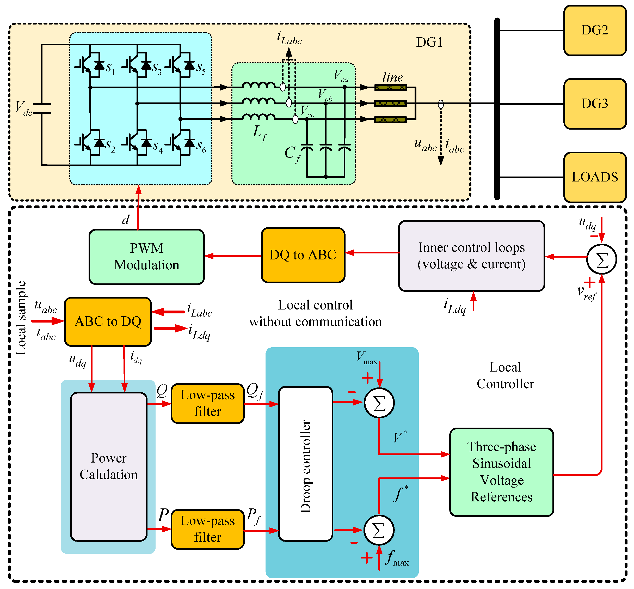
where , , , are the frequency reference, terminal voltage reference, active power output, reactive power output of the ith DG, respectively. The subscripts “max” and “min” indicate the corresponding maximum and minimum values. and are the output frequency and voltage of the DG under the no-load conditions. and are the output frequency and voltage of the DG under the full-load conditions. and are droop coefficients. The droop characteristics are shown in Figure 1.
and fed by the ith DG to the common bus through inductive lines are as follows:
where and are the terminal voltage of the ith DG and the voltage on the common bus. is the line equivalent inductance. is the voltage phase difference between and . When all the DGs get into the steady state, the power sharing could be obtained , note that, the proportional active power sharing is based on DGs’ power ratings.
3. Problem Formulation
3.1. Sufficient Conditions for the Economic Dispatch Problem
The total generation cost function for an MG can be expressed as:
where is the general comprehensive cost of the ith DG including maintenance cost, fuel cost, environmental cost, and so on, . The cost function is continuous in the operation range. The optimal problem without capacity constraints on the DGs is given as follows:
where is the total active load demands including the transmission loss. Suppose all the function are smooth and convex as , which represents the application conditions of the proposed scheme. This property is usually assumed (e.g., [36,37]). Thus, the optimization of (6) has a unique optimal solution.
3.2. Necessary Conditions for the Economic Dispatch Problem
Lagrangian method is adopted to find the optimal solution formulated in (6). The Lagrangian function is:
where is Lagrange multiplier. And then the necessary condition for optimality could be obtained as follows:
Simplifying (8) yields:
The total generation cost of the MG is minimized so long as the incremental costs of all the DGs are equal, i.e., the equal incremental cost principle.
4. Proposed P-f Scheme for Decentralized Economic Operation
4.1. Optimal Synchronous Operation
To realize the optimality condition in (9) without the need of communications, the droop control scheme for the economic operation of the MG is implemented as follows:
where is a constant for all the DGs, which is determined by the desired frequency ranges [, ] (e.g., ). and are the maximum and minimum frequencies allowed by the MG. When the MG gets into the steady state, the frequencies of all the DGs converge to the same value. By (10), the optimality condition (9) will be satisfied automatically. That is to say, the economic operation of the MG can be obtained by (10).
Note that the proposed droop control scheme in (10) only needs the local information of each DG, and communications between different DGs are not needed. Therefore, no matter whether any DG is added or removed, the optimality condition for economic operation holds always. In other words the plug-and-play of DGs is retained under the proposed droop control scheme (10).
Assume that the feasible region of DGs’ active power outputs is given by:
For illustration, the MG shown in Figure 2 is taken as an example. A typical general comprehensive cost function as [11,23,34] is used in this paper and the coefficients for different DGs are listed in Table 1. For convenience, p.u. values are used in this paper.
The P-f characteristic curves of the DGs under the droop control scheme in (10) are shown in Figure 3. The operation frequency of MG is determined by the balance level between the active power output of all DGs and the load demands . In cases when the MG is under heavy load or light load, the active power output of some DGs may reach its limits ( or ). However, it is proven in Section 5 that the power-angle steady condition will not be satisfied in theory when the active power output of any DG remains unchanged at its limits. Based on this reason, the definitions of OSO and SSO states of the MG are proposed in this paper.
In Figure 3, is used to denote the operation frequency of the MG in OSO states, in which the active power output of each DG in the MG locate in the range of [, ]. The detailed definition of and are presented in Section 4.2 and Figure 4. Define , . When the steady state MG operating frequency locates in , it is defined as OSO states. When the steady operation frequency of MG locates in , the operation states are defined as SSO states.
When the MG operates in OSO states, the droop control scheme in (10) is used. In cases when the MG operates in SSO states, a modified droop control scheme, as described in Section 4.2, is proposed as a tradeoff of between the economy and stability.
4.2. Suboptimal Synchronous Operation Considering Distributed Generators Capacity Limitations and Microgrid Stability
In the case of SSO, a modified droop control scheme for the economic operation of the MG is implemented as follows:
where and are two active power points, from which of the ith DG starts to change according to (13). is a value close to but larger than . is a value close to but smaller than . The OSO and SSO modes of the MG are connected at (, ) and (, ). and are the functions of , the design principles of which are illustrated in detail as follows.
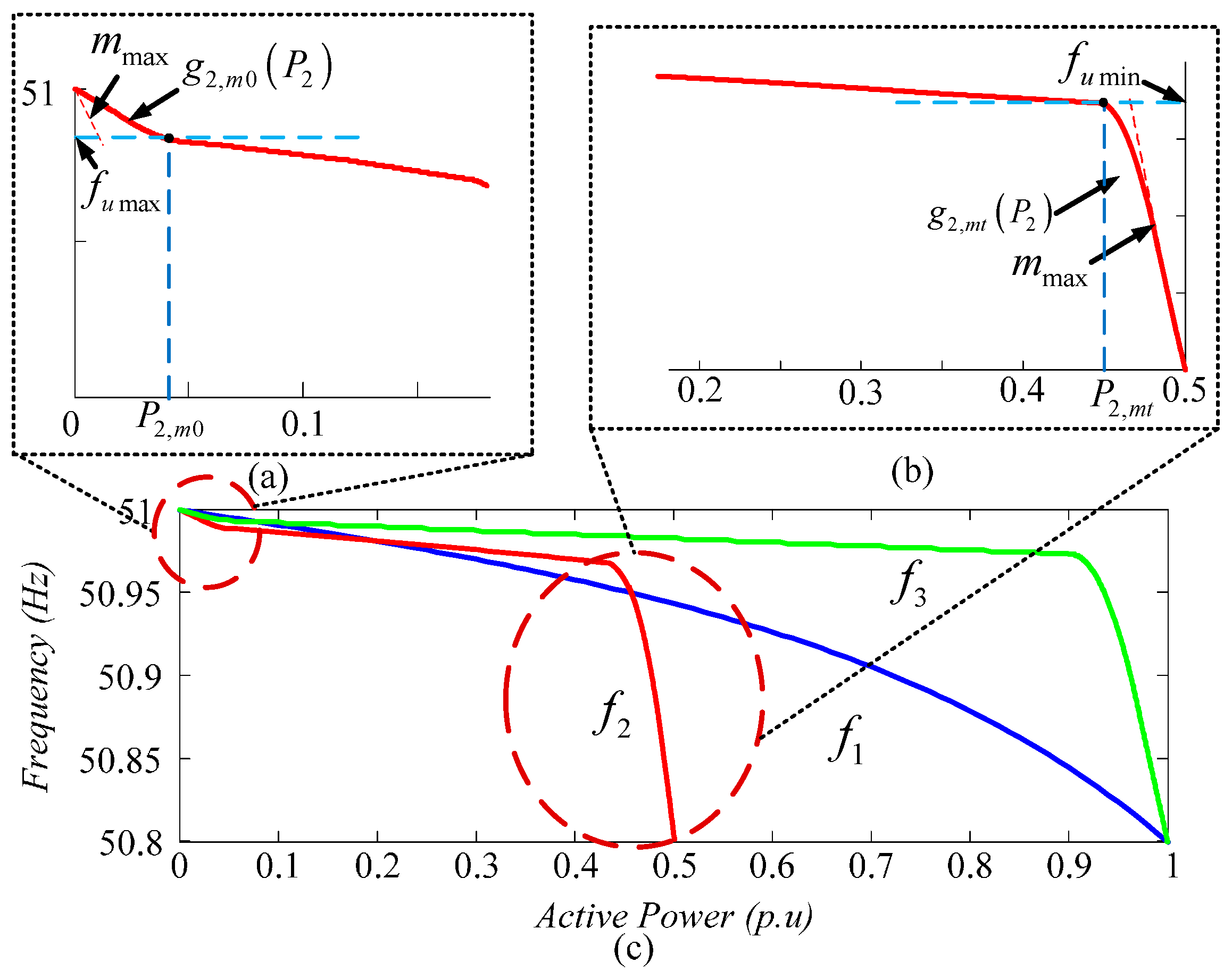
An example of the P-f characteristic curves of the DGs under the modified droop control scheme in (12) and (13) is shown in Figure 4. Take DG2 for instance. When locates in [,] or [,] required by the economic operation, the droop curve of DG2 should be modified as or , as shown in Figure 4a,b, respectively.
The design of and should satisfy the following requirements:
- (1)
- shall be smooth and continuous in the range of [, ], especially function should be continues at the connecting points and .
- (2)
- In order to obtain synchronous operation within DGs’ capacity limitations, should start from (Pi,min, fmax) and end at (Pi,max, fmin), namely gi,m0(Pi = Pi,max) = fmax, gi,mt(Pi = Pi,max) = fmin.
- (3)
- The droop coefficients should satisfy the stability constraints of the MG, i.e., . is the permissible maximum droop coefficient determined by the technical conditions of DGs and also by the requirement of a broad stability domain of the MG.
According to the above requirements, the mathematical descriptions of design principles of and are as follows:
It is obvious that, large is favourable for economic operation for MG. But an unreasonable may lead to the power-angle oscillation and even cause instability in the MG [38]. Therefore, should be selected as a tradeoff between economy and stability factors. In this paper, is set at
The optimal , , and can be designed through functional analysis method under the constraints of (14) and (15). For simplicity at the same time without losing effectiveness, the piecewise parabolic fitting method is adopted in this paper. For example, in our work, was set to , while was set to . Figure 4 shows the P-f characteristic curves obtained by the piecewise parabolic fitting method, which are used in the simulation and experiment work.
5. Small Signal Analysis
To investigate the stability of the MG, the small-signal analysis method [39,40] is applied. Without loss of generality, the equivalent circuit of the MG composed of DGs shown in Figure 5 is studied. In Figure 5, is the terminal voltage of the ith DG, is the voltage of the common bus, and are the phase angles of the corresponding voltages, is the equivalent admittance between the ith DG and the common bus, and is the equivalent admittance of the comprehensive load.
5.1. Small Signal Analysis for the Necessity of Modifications
Based on Kirchhoff current laws, the common bus voltage can be expressed as:
where:
and can be rewritten as:
where and are the modulus and angle of , respectively.
The output active power and reactive power of the ith DG is defined as [41]:
where is the phase angle difference between and .
With , , , and (16)–(20), it is easy to obtain the new expressions of the output active and reactive power of the ith DG without the appearance of and :
In both high and medium voltage systems, . Consequently, . Compared with and respectively, and can be neglected. As a result, (21) and (22) can be simplified as:
Suppose that the output frequency reference is tracked by the ith DG without the steady-state error. Then the proposed droop control scheme in (12) can be written as follows:
where is the output angular frequency of the ith DG, .
Assume that is the MG synchronous operation angle frequency in the steady state. Let , and denote , then (25) can be rewritten as:
Since P-f has a much slower dynamic characteristic compared with the voltage dynamics, the voltage dynamics can be neglected when the P-f relationship is analyzed. Linearization of (23) and (26) near the equilibrium point in the Laplace domain yields:
where ‘°’ is the corresponding value around the equilibrium point. By substituting (27) into (28), and neglecting , we can get:
Expressing (30) in matrix form:
where , , , .
Obviously, . If , is a Laplacian matrix, the eigenvalues of are in the left half-plane [42]. Consequently, the related system is stable. In order to ensure , there should be:
Due to the fact that , . In order to ensure (32), there should be .
To ensure , (12) should be a strictly monotonically decreasing function on [, ]. If not, converting the nonmonotonic parts into monotonic manner is recommended for stability reasons. Without loss of generality, the conditions mentioned above can also be applied to guide the construction of P-f droop scheme for other objectives.
5.2. Root-Locus Analysis for the Proposed Scheme in the Considered Microgrid
The resistor-inductance line and output filter are considered to depict the root locus diagrams. And the filtered active power and reactive power with the output filter can be rewritten as:
where is the s-domain transfer function of the output filter, is the cutoff frequency of the filter and the same is assumed for all DGs.
The small-signal model of (23), (24), (26), (33) and (34) around the stable operating point is given as follows:
where:
and is Q-V droop coefficients.
To test the stability of the proposed droop control scheme, the root-locus method is used for the considered MG shown in Figure 2. And resistance-inductance load is assumed. The root locus diagram by changing the load resistance and the line coupling inductance is studied.
Figure 6 shows the root locus diagram with the load resistance changing from 50 Ω to 100 Ω (i.e., changes from 1.08 p.u. to 2.16 p.u., assuming the voltage of the common bus is invariant), while the load inductance is set 6 mH, and the equivalent line coupling impedance between the ith DG and the common bus is set , . In Figure 6, there is a single eigenvalue at zero corresponding to rotational symmetry, as also depicted in [43]. And the rest eigenvalues are in the left half-plane. Thus the system is stable.
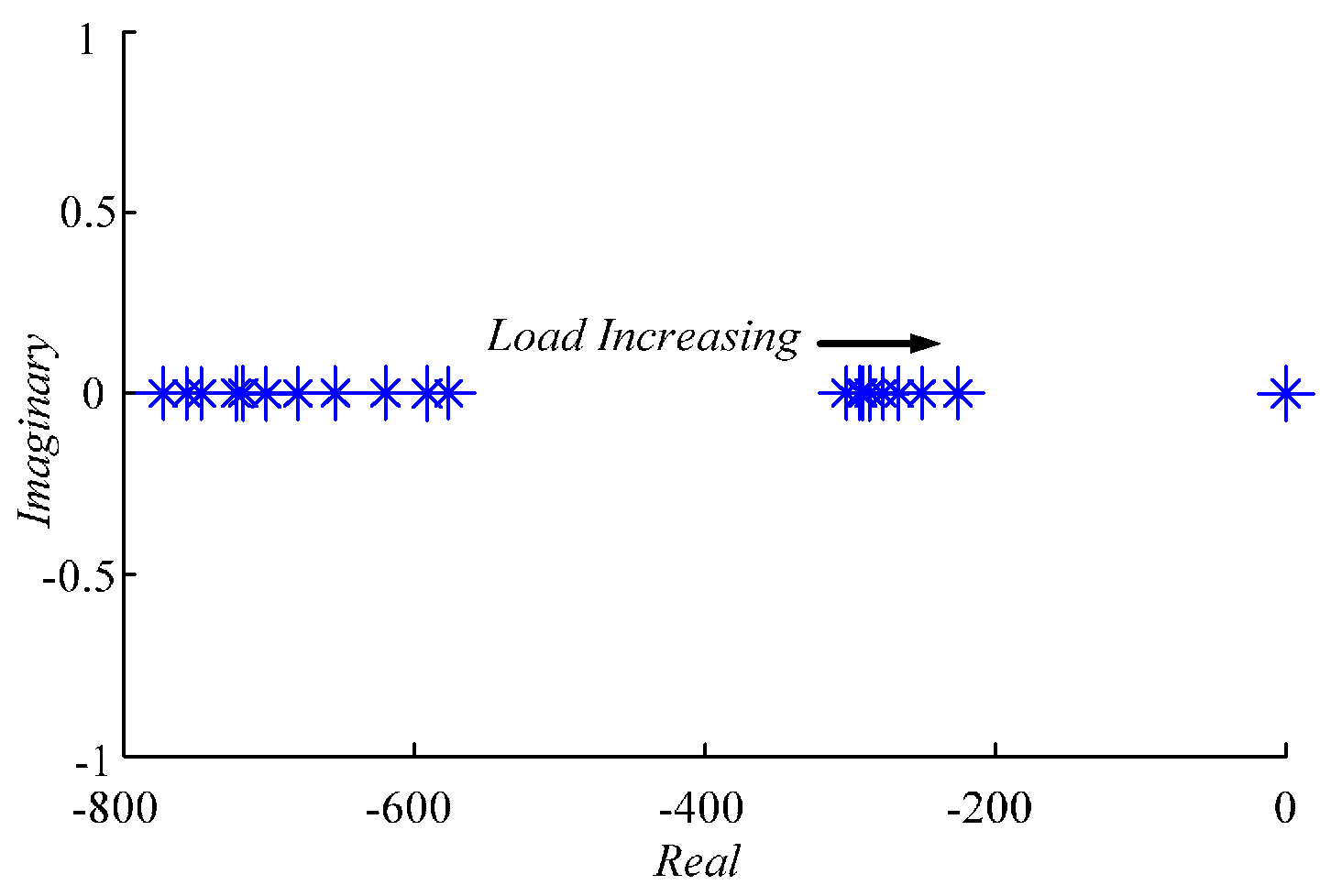
Figure 7 shows the root locus diagram as decreases from 3 mH to 0.1 mH, while , . In this case, there is also an eigenvalue at zero, as also depicted in [43]. When the value of Xi decreases, the poles move from the left half plane to the right half plane. Finally the system loses its stability. In this example, the stable operation can be ensured with the proposed scheme when the line coupling inductance including the output filter is more than 0.14 mH. That is to say, the total line coupling inductance shouldn’t be too small for stability reason, which is often ignored in most literatures.
6. Simulation Validations
To verify the performance of the proposed scheme, simulations are carried out in Matlab/Simulink. The setup for simulation is shown in Figure 8, and the related parameters are shown in Table 2. The traditional Q-V droop control in (2) is applied to the simulations.
6.1. Case1: Necessity for the Modifications When Considering DGs Capacity Limitations
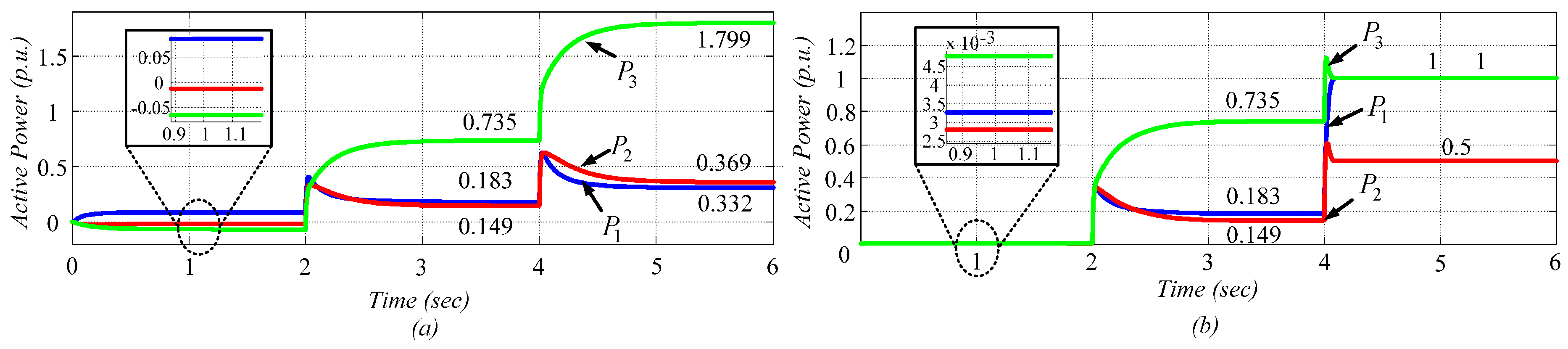
In order to present the necessity for modifying (10) for economic operation with considering DGs’ capacity limitations via decentralized approach, (10) and (12) are tested and compared. The active power allocation among the DGs for the scheme of (10) and (12) are shown in Figure 9a,b, respectively. In the interval [0 s, 2 s] under the light load demand, the output active power of DG3 with the scheme (10) is negative shown in Figure 9a, which is dangerous and even is prone to destructive results. However, the output active power of all DGs with the proposed scheme (12) is desired positive for all DGs in Figure 9b.
In the interval [2 s, 4 s] under the medium load demand, the output active power of all DGs with the droop scheme (10) and (12) are same, which is related to OSO conditions. When a full load appears in the interval [4 s, 6 s], the output of DG3 with (10) is 1.799 p.u. (It exceeds its maximum capacity 1 p.u.), which is not permissible. However, the proposed droop scheme (12) could control all DGs in their maximum capacity (, , ).
Accordingly, the simulation results verified that the proposed droop scheme (12) could protect generators from being destroyed due to overloading or negative power impact.
6.2. Case 2: Economy Comparisons between the Proposed P-f Scheme and the Interior Point Method
For comparison, the economical operation solutions through the interior point method [44] are depicted in Figure 10a. The corresponding TAGC of the MG is shown in Figure 10b. As shown in Figure 10a, in case when the DG active power output reaches its maximum value as load increases, . Then is not satisfied, which is unfavourable for system stability. Thus, modifications are necessary for stability reasons. Besides, in order to achieve the optimal economic operation, the centralized controllers with communications are usually needed.
Under the same setup, the economical operation solutions of the proposed droop control scheme using (12) are shown in Figure 10c. Although there are some subtle distinctions between Figure 10a,c, the distinctions of TAGC under the two schemes as shown in Figure 10d is not obvious. In most cases, the TAGC of the proposed scheme (12) are in good agreement with that in Figure 10b. Based on the simulation results, it is verified that the proposed droop control scheme (12) could achieve satisfactory economic operations even in the presence of capacity limitations.
6.3. Case 3: Performance of the Proposed P-f Scheme
To verify the performance of the proposed P-f scheme, simulation is implemented as load step changes at 2 s and 4 s shown in Figure 11a. When the MG gets into the steady state, the frequency converges to a constant as shown in Figure 11b. Figure 11c shows the behavior of during the transient process. And active power allocation among DGs through the proposed droop control scheme is shown in Figure 11d. The simulation results with the proposed scheme are in accordance with the theoretical results as shown in Figure 10a, the OSO operation is obtained in the first and second interval, i.e., 0–2 s and 2–4 s, respectively. The SSO operation is realized in the third interval, i.e., 4–6 s, as a tradeoff between economy and stability.
From the simulation results, it is verified that the proposed P-f scheme does very well in response to the step change of the load. The frequency could be controlled within the allowable ranges. And all the DG active power limitations are not conflicted.
6.4. Case 4: Plug and Play Capability of the Proposed P-f Scheme
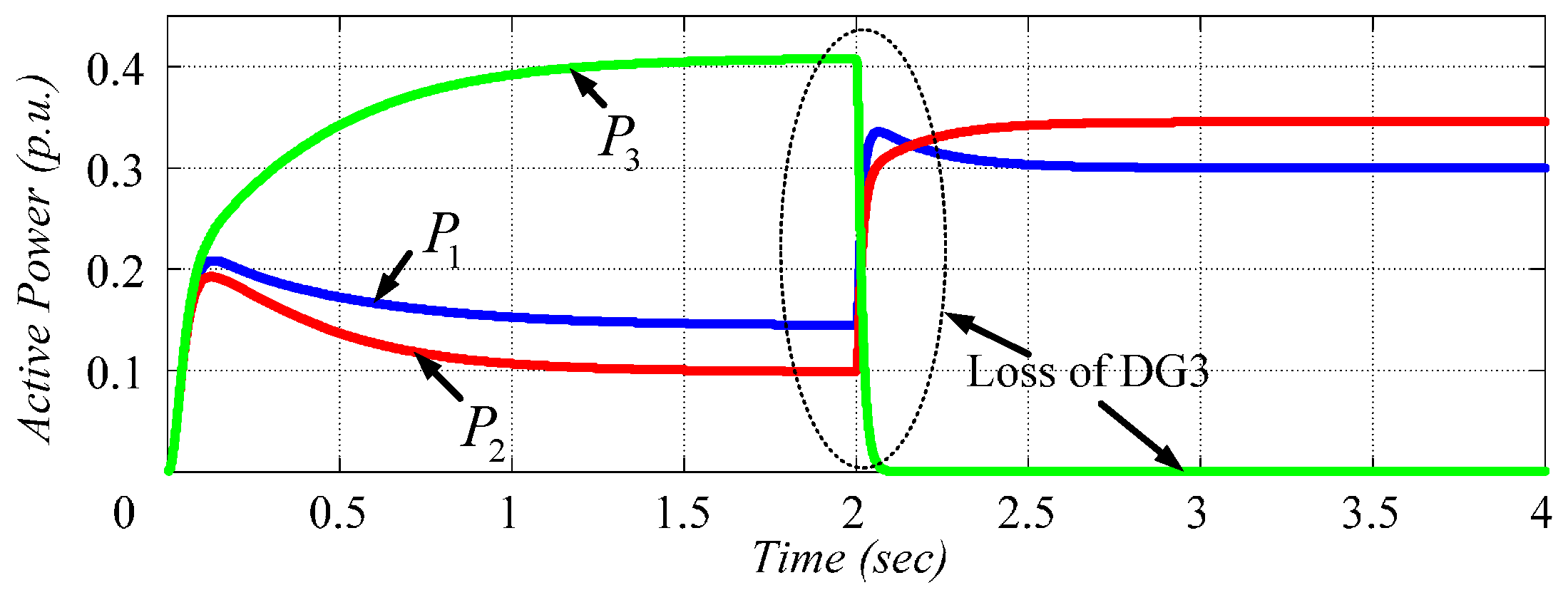
In this case, the proposed P-f scheme is implemented under a certain load, when DG3 is suddenly lost at 2 s. From the simulation result in Figure 12, the load could be shared automatically among the rest available DGs according to their economic droop curves. Therefore, it is verified that the proposed P-f scheme holds the capability of plug and play, while maintaining the economical allocation of the load.
7. Experimental Results
A MG experimental prototype was built to verify the effectiveness of the proposed P-f scheme, as shown in Figure 13. Limited by the experimental conditions, a MG consisting of two DGs was tested. The two DGs are realized utilizing single phase voltage source inverters, which are controlled by digital signal processors (TMS320f28335) with a sampling rate at 12.8 kHz. The coefficients of the DGs’ generation cost functions are as listed in Table 1. And the experimental parameters are shown in Table 3. The experiments are carried out in terms of the proposed P-f scheme as the load of the MG changes. The traditional Q-V droop control in (2) is applied to the experiments.
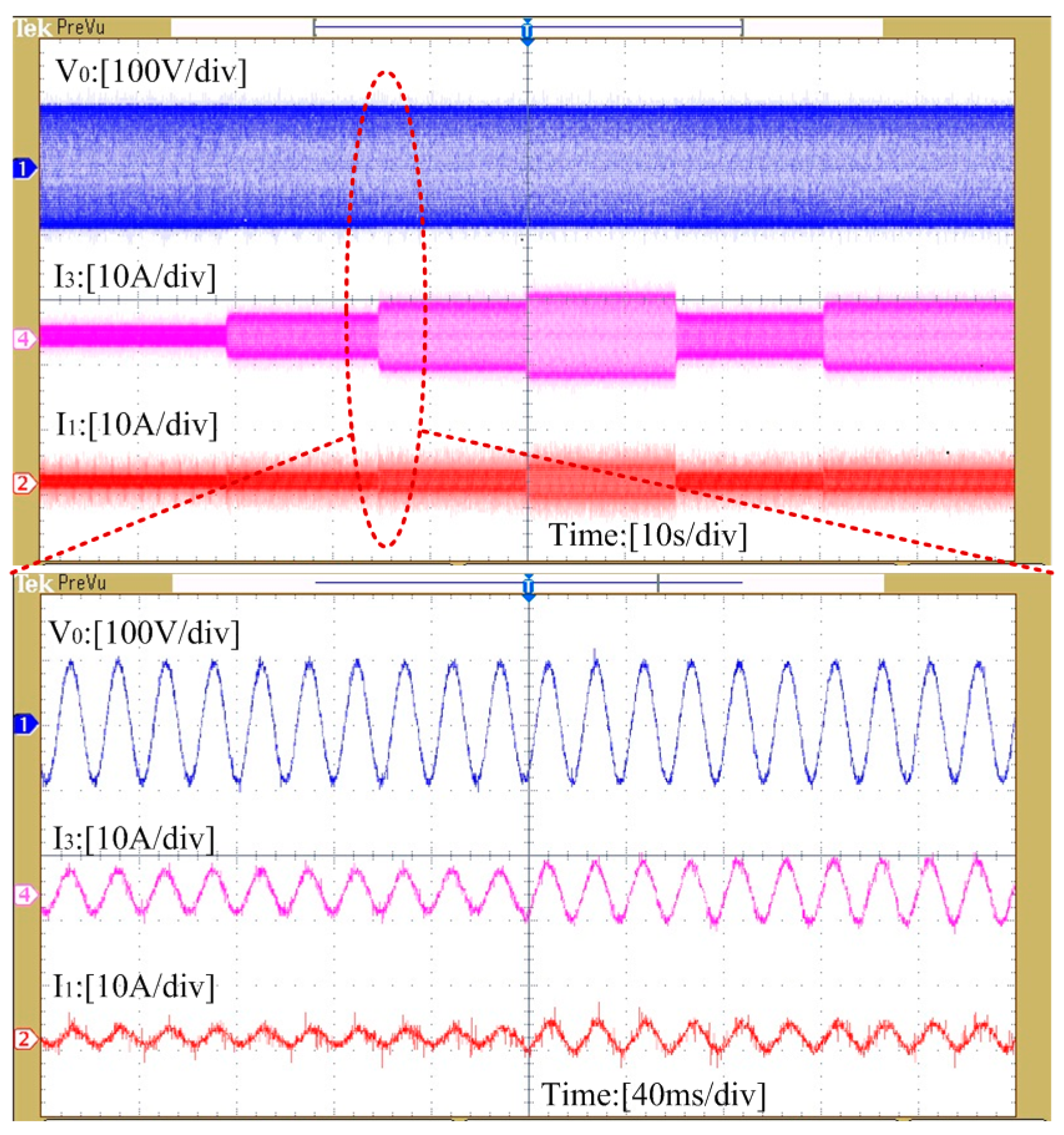
7.1. Case 1: Performance of the Proposed P-f scheme with Equally Rated DGs (DG1 and DG3)
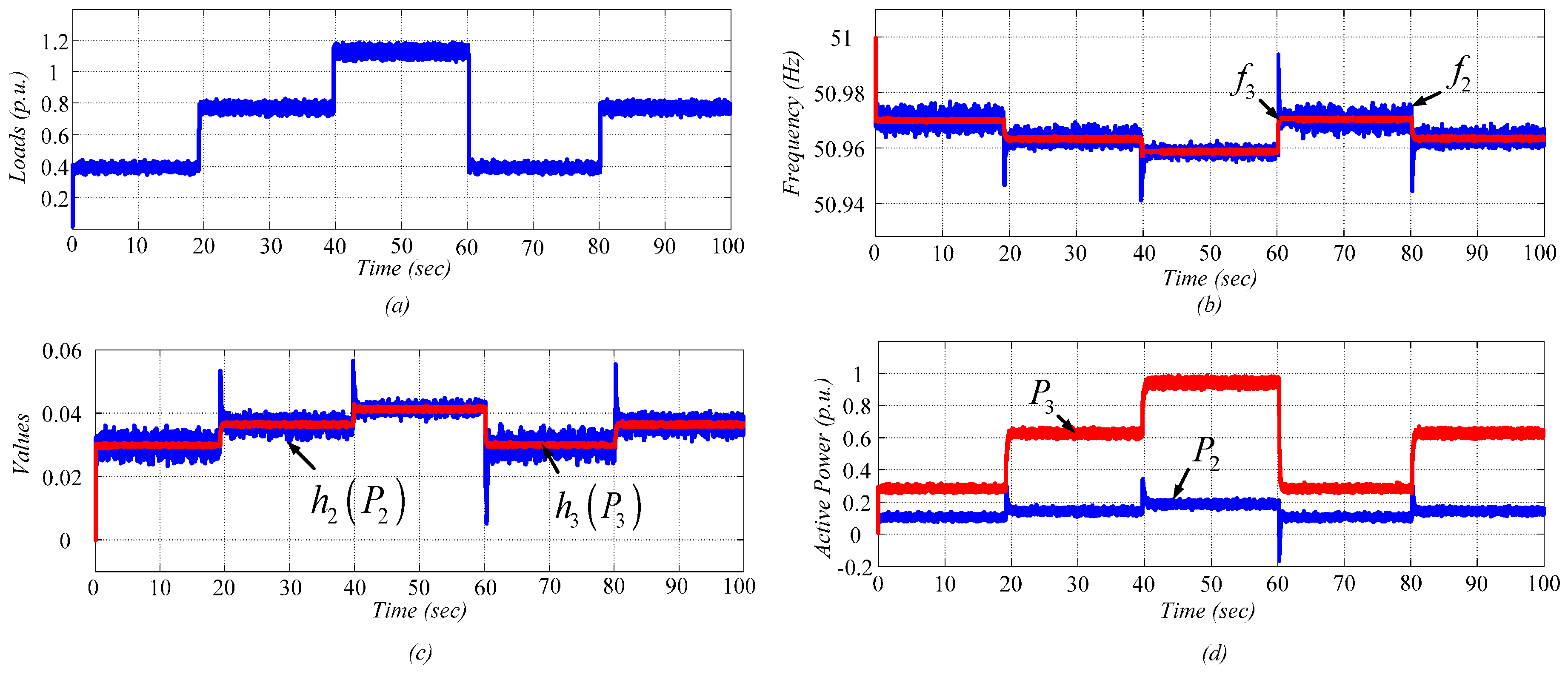
In this experimental case, the generation cost function coefficients of the DG1 and DG3, as listed in Table 1, are used to verify the proposed scheme. DG1 and DG3 having equal rated capacity is assumed at 1 p.u. The voltage waveforms on the common bus and the current waveforms of the DGs based on the proposed P-f scheme are shown in Figure 14. The waveforms of the load, frequency, and active power allocations of DG1 and DG3 based on the proposed P-f scheme are illustrated in Figure 15. Since the frequency is applied as a carrier in the proposed P-f scheme, values of all the DGs are equal even when the load changes, as shown in Figure 15c. Due to the difference of the hardware, the disturbance in the red and blue waveforms is different as shown in Figure 15b,c. And the optimal power dispatch is achieved according to their generation cost function, as shown in Figure 15d, while the smooth and stable operation is maintained even with the capacity limitation constraints.
7.2. Case 2: Performance of the Proposed P-f Scheme with Unequally Rated DGs (DG2 and DG3)
In this test, the generation cost function coefficients of the DG2 and DG3, as listed in Table 1, are used to verify the proposed scheme. DG2 and DG3 having unequal rated capacity are assumed (, ). The waveforms of the voltage on the common bus and the DGs’ current are as shown in Figure 16. The corresponding waveforms of the load, frequency, and active power allocations of DG2 and DG3 are illustrated in Figure 17. Again, the optimal economic power sharing is obtained as the frequency converges. In Figure 17d, the negative power spike flashing at 60 s is caused by the fast dynamic process without affecting the steady state performance. The experimental results verified that the proposed P-f scheme can maintain the smooth stabilization in presence of capacity limitations with unequally rated DGs even when the load has step changes.
8. Conclusions
In this paper, a P-f droop scheme for MGs is proposed to reduce the MG TAGC via a decentralized approach. The sufficient conditions for MG economic operation under the proposed P-f droop method are explored by the small-signal analysis method. Because the implementation of the proposed P-f scheme only needs the local information of each DG, communications are not needed. Therefore, it represents a reliable and low-cost solution. In addition, to deal with the limitations of DGs’ capacity, a modification method is proposed, which guarantees the synchronization and stability of the MGs. Both simulation and experimental results have verified the effectiveness of the proposed scheme.
Acknowledgments
This work was supported by the National Natural Science Foundation of China under Grant No. 61573384, and the Natural Science Foundation of Hunan Province of China under Grant No. 2016JJ1019.
Author Contributions
Lang Li conceived the main idea and wrote the manuscript with guidance from Hua Han and Mei Su. Lina Wang, Yue Zhao and Josep M. Guerrero reviewed the work and gave helpful improvement suggestions.
Conflicts of Interest
The authors declare no conflict of interest.
References
- Yu, Z.; Ai, Q.; Gong, J.; Piao, L. A novel secondary control for microgrid based on synergetic control of multi-agent system. Energies 2016, 9, 243. [Google Scholar] [CrossRef]
- Camblong, H.; Etxeberria, A.; Ugartemendia, J.; Curea, O. Gain Scheduling Control of an Islanded Microgrid Voltage. Energies 2014, 7, 4498–4518. [Google Scholar] [CrossRef]
- Hu, S.-H.; Lee, T.-L.; Kuo, C.-Y.; Guerrero, J.M. A Riding-through Technique for Seamless Transition between Islanded and Grid-Connected Modes of Droop-Controlled Inverters. Energies 2016, 9, 732. [Google Scholar] [CrossRef]
- Chen, C.; Duan, S.; Cai, T. Smart energy management system for optimal microgrid economic operation. IET Renew. Power Gener. 2011, 5, 258–267. [Google Scholar] [CrossRef]
- Fei, W.; Duarte, J. Grid-interfacing converter systems with enhanced voltage quality for microgrid application concept and implementation. IEEE Trans. Power Electron. 2011, 26, 3501–3513. [Google Scholar]
- Lim, Y.; Kim, H.M.; Kinoshita, T. Distributed load-shedding system for agent-based autonomous microgrid operations. Energies 2014, 7, 385–401. [Google Scholar] [CrossRef]
- Lu, X.; Wan, J. Modeling and Control of the Distributed Power Converters in a Standalone DC Microgrid. Energies 2016, 9, 217. [Google Scholar] [CrossRef]
- Lopes, J.P.; Moreira, C.L.; Madureira, A.G. Defining Control Strategies for MicroGrids Islanded Operation. IEEE Trans. Power Syst. 2006, 21, 916–924. [Google Scholar] [CrossRef]
- Nikmehr, N.; Ravadanegh, S.N. Optimal Power Dispatch of Multi-Microgrids at Future Smart Distribution Grids. IEEE Trans. Smart Grid 2015, 6, 1648–1657. [Google Scholar] [CrossRef]
- Barklund, E.; Pogaku, N.; Prodanovic, M.; Hernandez-Aramburo, C.; Green, T.C. Energy management in autonomous microgrid using stability-constrained droop control of inverters. IEEE Trans. Power Electron. 2008, 23, 2346–2352. [Google Scholar] [CrossRef]
- Nutkani, I.U.; Loh, P.; Wang, P.; Blaabjerg, F. Cost-prioritized droop schemes for autonomous AC microgrids. IEEE Trans. Power Electron. 2015, 30, 1109–1119. [Google Scholar] [CrossRef]
- Li, J.; Wei, W.; Xiang, J. A Simple Sizing Algorithm for Stand-Alone PV/Wind/Battery Hybrid Microgrids. Energies 2012, 5, 5307–5323. [Google Scholar] [CrossRef]
- Song, N.O.; Lee, J.H.; Kim, H.M.; Im, Y.H.; Lee, J.Y. Optimal energy management of multi-microgrids with sequentially coordinated operations. Energies 2015, 8, 8371–8390. [Google Scholar] [CrossRef]
- Hussain, A.; Bui, V.-H.; Kim, H.-M. Robust Optimization-Based Scheduling of Multi-Microgrids Considering Uncertainties. Energies 2016, 9, 278. [Google Scholar] [CrossRef]
- Che, L.; Shahidehpour, M. DC Microgrids: Economic Operation and Enhancement of Resilience by Hierarchical Control. IEEE Trans. Smart Grid 2014, 5, 2517–2526. [Google Scholar]
- Che, L.; Shahidehpour, M.; Alabdulwahab, A.; Al-Turki, Y. Hierarchical Coordination of a Community Microgrid with AC and DC Microgrids. IEEE Trans. Smart Grid 2015, 6, 3042–3051. [Google Scholar] [CrossRef]
- Li, C.; De Bosio, F.; Chen, F.; Chaudhary, S.K.; Vasquez, J.C.; Guerrero, J.M. Economic Dispatch for Operating Cost Minimization Under Real-Time Pricing in Droop-Controlled DC Microgrid. IEEE J. Emerg. Sel. Top. Power Electron. 2017, 5, 587–595. [Google Scholar] [CrossRef]
- Tsikalakis, A.G.; Hatziargyriou, N.D. Centralized control for optimizing microgrids operation. IEEE Trans. Energy Convers. 2008, 23, 241–248. [Google Scholar] [CrossRef]
- Katiraei, F.; Iravani, R.; Hatziargyriou, N.; Dimeas, A. Microgrids management. IEEE Power Energy Mag. 2008, 6, 54–65. [Google Scholar] [CrossRef]
- Guerrero, J.M.; Chandorkar, M.; Lee, T.-L. Advanced control architectures for intelligent microgrids—Part I: Decentralized and hierarchical control. IEEE Trans. Ind. Electron. 2013, 60, 1254–1262. [Google Scholar] [CrossRef]
- Olivares, D.E.; Mehrizi-Sani, A.; Etemadi, A.H. Trends in microgrid control. IEEE Trans. Smart Grid 2014, 5, 1905–1919. [Google Scholar] [CrossRef]
- Yazdanian, M.; Mehrizi-Sani, A. Distributed control techniques in microgrids. IEEE Trans. Smart Grid 2014, 5, 2901–2909. [Google Scholar] [CrossRef]
- Zhang, W.; Liu, W.; Wang, X.; Liu, L.; Ferrese, F. Online optimal generation control based on constrained distributed gradient algorithm. IEEE Trans. Power Syst. 2015, 30, 35–45. [Google Scholar] [CrossRef]
- Zhang, Z.; Chow, M.-Y. Convergence analysis of the incremental cost consensus algorithm under different communication network topologies in a smart grid. IEEE Trans. Power Syst. 2012, 27, 1761–1768. [Google Scholar] [CrossRef]
- Yang, S.; Tan, S.; Xu, J.-X. Consensus based approach for economic dispatch problem in a smart grid. IEEE Trans. Power Syst. 2013, 28, 4416–4426. [Google Scholar] [CrossRef]
- Yan, B.; Wang, B.; Zhu, L. A novel, stable, and economic power sharing scheme for an autonomous microgrid in the energy internet. Energies 2015, 8, 12741–12764. [Google Scholar] [CrossRef]
- Ahn, C.; Peng, H. Decentralized and real-time power dispatch control for an islanded microgrid supported by distributed power sources. Energies 2013, 6, 6439–6454. [Google Scholar] [CrossRef]
- Cosse, R.E.; Alford, M.D.; Hajiaghajani, M.; Hamilton, E.R. Turbine/generator governor droop/isochronous fundamentals—A graphical approach. In Proceedings of the Petroleum and Chemical Industry Conference, Toronto, ON, Canada, 19–21 September 2011. [Google Scholar]
- Jaleeli, N.; VanSlyck, L.S.; Ewart, D.N.; Fink, L.H.; Hoffmann, A.G. Understanding automatic generation control. IEEE Trans. Power Syst. 1992, 7, 1106–1122. [Google Scholar] [CrossRef]
- Guerrero, J.M.; Hang, L.; Uceda, J. Control of distributed uninterruptible power supply systems. IEEE Trans. Ind. Electron. 2008, 55, 2845–2859. [Google Scholar] [CrossRef]
- Lee, C.T. A new droop control method for the autonomous operation of distributed energy resource interface converters. IEEE Trans. Power Electron. 2013, 28, 1980–1993. [Google Scholar] [CrossRef]
- Haddadi, A.; Joos, G. Load sharing of autonomous distribution-level microgrids. In Proceedings of the Power and Energy Society General Meeting, San Diego, CA, USA, 24–29 July 2011. [Google Scholar]
- Mohamed, Y.A.-R.I.; El-Saadany, E.F. Adaptive decentralized droop controller to preserve power sharing stability of paralleled inverters in distributed generation microgrids. IEEE Trans. Power Electron. 2008, 23, 2806–2816. [Google Scholar] [CrossRef]
- Nutkani, I.U.; Loh, P.C.; Blaabjerg, F. Droop scheme with consideration of operating costs. IEEE Trans. Power Electron. 2014, 29, 1047–1052. [Google Scholar] [CrossRef]
- Cingoz, F.; Elrayyah, A.; Sozer, Y. Plug and play nonlinear droop construction scheme to optimize microgrid operations. In Proceedings of the Energy Conversion Congress and Exposition (ECCE), Pittsburgh, PA, USA, 24–29 July 2011. [Google Scholar]
- Xiao, L.; Boyd, S. Optimal scaling of a gradient method for distributed resource allocation. J. Optim. Theory Appl. 2006, 129, 469–488. [Google Scholar] [CrossRef]
- Ghadimi, E.; Johansson, M.; Shames, I. Accelerated gradient methods for networked optimization. In Proceedings of the American Control Conference, San Francisco, CA, USA, 29 June–1 July 2011. [Google Scholar]
- Dong, J.; Zhang, C.-J.; Meng, X.-M.; Guo, Z.-N.; Kan, Z.-Z. Modeling and stability analysis of autonomous microgrid composed of inverters based on improved droop control. In Proceedings of the International Power Electronics and Application Conference and Exposition, Shanghai, China, 5–8 November 2014. [Google Scholar]
- Pogaku, N.; Prodanovic, M.; Green, T. Modeling, analysis and testing of autonomous operation of an inverter-based microgrid. IEEE Trans. Power Electron. 2007, 22, 613–625. [Google Scholar] [CrossRef]
- Guo, X.Q.; Lu, Z.G.; Wang, B.C. Dynamic Phasors-Based Modeling and Stability Analysis of Droop-Controlled Inverters for Microgrid Applications. IEEE Trans. Smart Grid 2014, 5, 2980–2987. [Google Scholar] [CrossRef]
- Palizban, O.; Kauhaniemi, K. Hierarchical control structure in microgrids with distributed generation: Island and grid-connected mode. Renew. Sustain. Energy Rev. 2015, 44, 797–813. [Google Scholar] [CrossRef]
- Reza, O.S.; Richard, M.M. Consensus Problems in Networks of Agents with Switching Topology and Time-Delays. IEEE Trans. Autom. Control 2004, 49, 1520–1533. [Google Scholar]
- Simpson-Porco, J.W.; Dörfler, F.; Bullo, F. Synchronization and power sharing for droop-controlled inverters in islanded microgrids. Automatica 2013, 49, 2603–2611. [Google Scholar] [CrossRef]
- Byrne, C.L. Iterative Optimization. In A First Course in Optimization; CRC Press: Lowell, MA, USA, 2014. [Google Scholar]
Figure 1.
Traditional droop scheme: (a) P-f characteristic; and (b) Q-V characteristic.
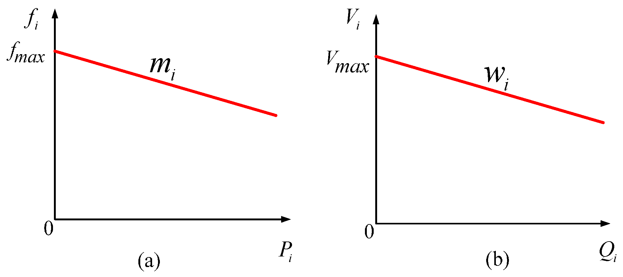
Figure 2.
A conceptual diagrams of a typical AC microgrid (MG).

Figure 3.
Proposed droop scheme without modifications for the considered AC MGs.
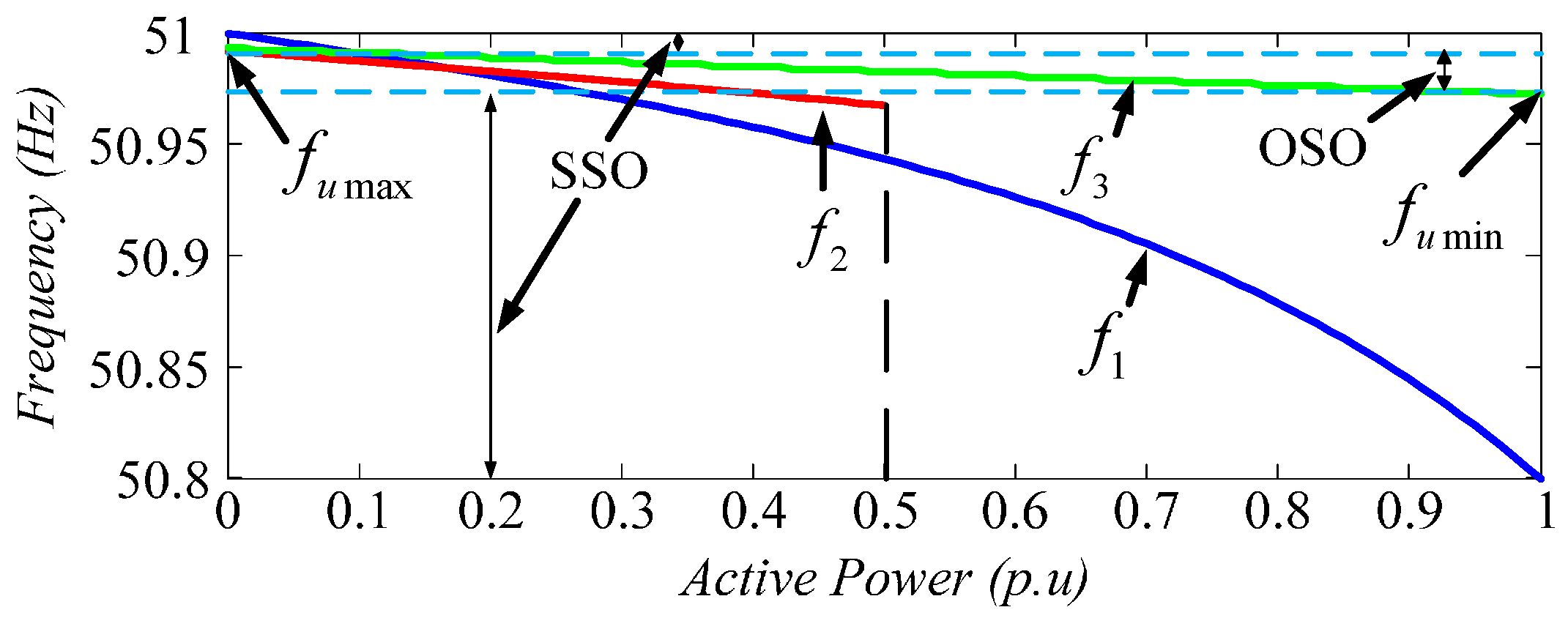
Figure 4.
P-f characteristic curves of the distributed generations (DGs): (a) a zoomed-in portion of P-f characteristic curves of DG2 when locates in the range of [, ]; (b) a zoomed-in portion of P-f characteristic curves of DG2 when locates in the range of [, ]; and (c) P-f characteristic curves of the DGs under the proposed scheme.

Figure 5.
Equivalent circuit of an n-DG MG.
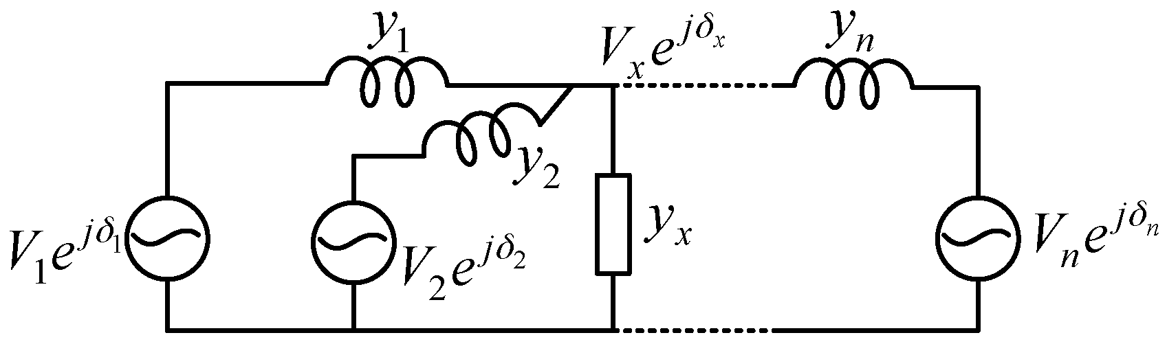
Figure 6.
Root locus as the load resistance increases from 50 Ω to 100 Ω.

Figure 7.
Root locus by decreasing the line coupling inductance.
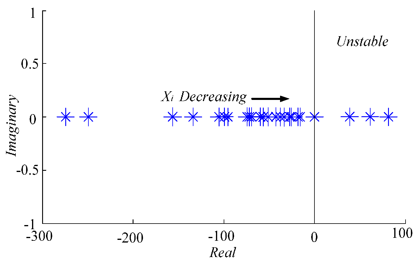
Figure 8.
Scaled-down simulation AC MGs.

Figure 9.
Variations of active power with the scheme of (a) without modification; and (b) with modification.
Figure 9.
Variations of active power with the scheme of (a) without modification; and (b) with modification.

Figure 10.
Power allocation results (a) power allocation among DGs through the interior point method; (b) total active generation cost (TAGC) of the interior point method; (c) power allocation among DGs through the proposed droop control scheme; (d) TAGC of the proposed droop control scheme.
Figure 10.
Power allocation results (a) power allocation among DGs through the interior point method; (b) total active generation cost (TAGC) of the interior point method; (c) power allocation among DGs through the proposed droop control scheme; (d) TAGC of the proposed droop control scheme.
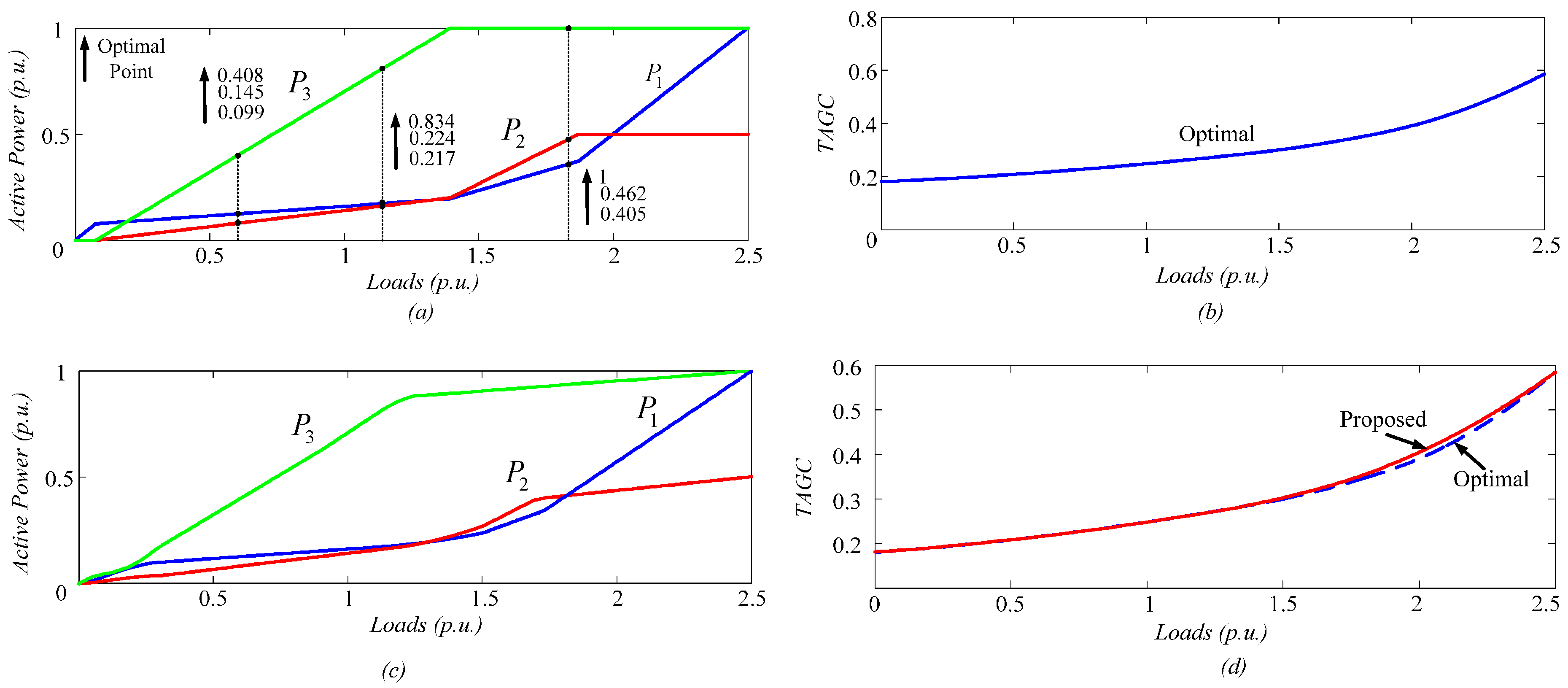
Figure 11.
Variations of (a) loads; (b) frequency; (c) ; and (d) active power output of DGs.

Figure 12.
Variations of active power with losing DG3.

Figure 13.
Experimental prototype setup of an AC MG.
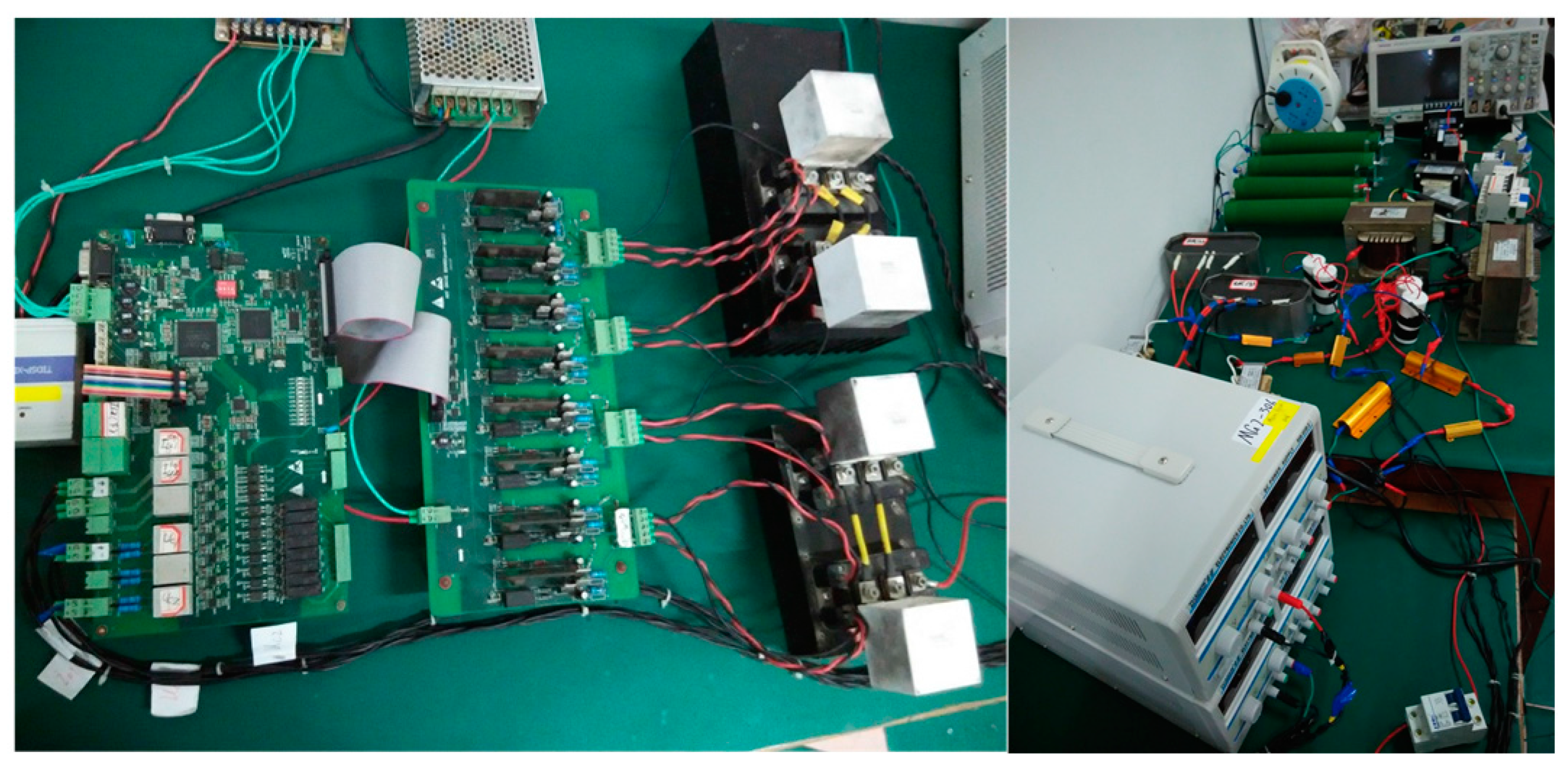
Figure 14.
Experimental voltage and current waveforms.

Figure 15.
Waveforms of (a) the load; (b) frequency; (c) values; and (d) DGs’ active power outputs.
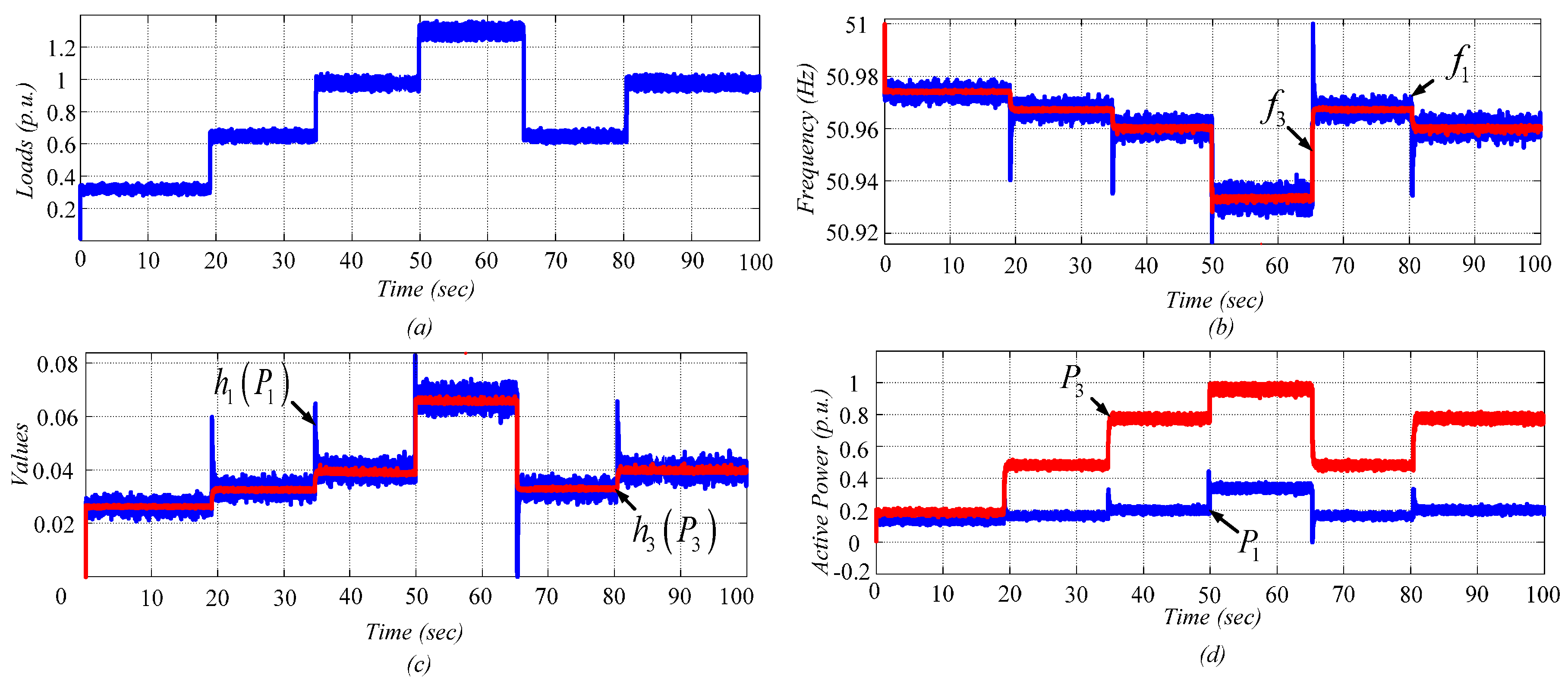
Figure 16.
Experimental voltage and current waveforms.
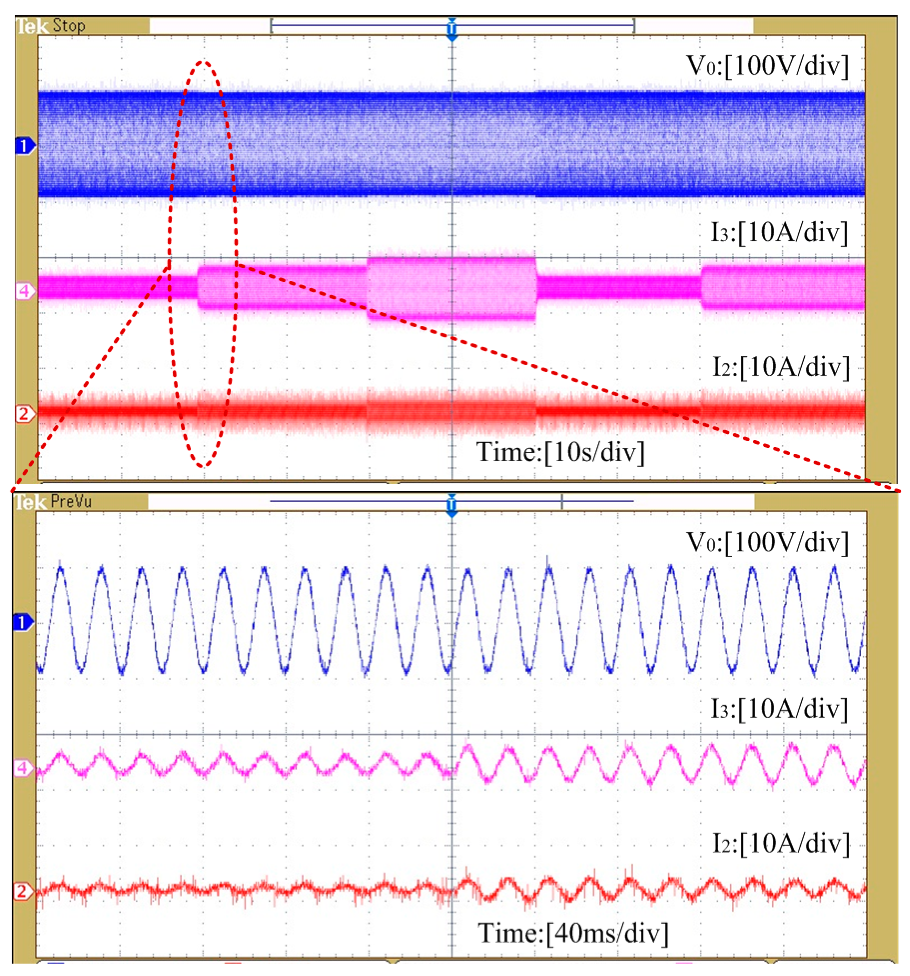
Figure 17.
Variations of (a) loads; (b) frequency; (c) ; and (d) DGs active power over time.

Table 1.
Cost coefficients for the considered AC MGs.
| DG | ||||
|---|---|---|---|---|
| DG1 | 0.253 | 0.010 | 1.0 × 10⁻³ | 3.33 |
| DG2 | 0.150 | 0.049 | 0.4 × 10⁻³ | 2.86 |
| DG3 | 0.030 | 0.049 | 0 | 0 |
Table 2.
Parameters for simulation.
| Parameter | Values | Parameter | Values |
|---|---|---|---|
| Frequency | [50.8, 51] Hz | Max () | 0.5 p.u. |
| Voltage | [0.95, 1.05] p.u. | Max () | 1 p.u. |
| Basic voltage | 380 V | Max ) | 0.563 |
| Basic power | 4 kW | Max () | 0.359 |
| Max () | 1 p.u. | Max () | 0.109 |
Table 3.
Parameters for experiments.
| Parameters | Value | Parameters | Value |
|---|---|---|---|
| Frequency | [50.8, 51] Hz | Filter inductor | 1 mH |
| Voltage | [0.95, 1.05] p.u. | Filter capacitor | 20 µF |
| Basic voltage | 96V (Line rms) | Line 3 inductor | 0.6 mH |
| Basic power | 400 W | Line 1, 2 inductor | 0.3 mH |
© 2017 by the authors. Licensee MDPI, Basel, Switzerland. This article is an open access article distributed under the terms and conditions of the Creative Commons Attribution (CC BY) license (http://creativecommons.org/licenses/by/4.0/).
Share and Cite
MDPI and ACS Style
Han, H.; Li, L.; Wang, L.; Su, M.; Zhao, Y.; Guerrero, J.M. A Novel Decentralized Economic Operation in Islanded AC Microgrids. Energies 2017, 10, 804. https://doi.org/10.3390/en10060804
AMA Style
Han H, Li L, Wang L, Su M, Zhao Y, Guerrero JM. A Novel Decentralized Economic Operation in Islanded AC Microgrids. Energies. 2017; 10(6):804. https://doi.org/10.3390/en10060804
Chicago/Turabian StyleHan, Hua, Lang Li, Lina Wang, Mei Su, Yue Zhao, and Josep M. Guerrero. 2017. "A Novel Decentralized Economic Operation in Islanded AC Microgrids" Energies 10, no. 6: 804. https://doi.org/10.3390/en10060804
Note that from the first issue of 2016, this journal uses article numbers instead of page numbers. See further details here.