
Pressure Losses in Multiple-Elbow Paths and in V-Bends of Hydraulic Manifolds


Engineering Department Enzo Ferrari, via P. Vivarelli 10, 41125 Modena, Italy
*
Author to whom correspondence should be addressed.
Energies 2017, 10(6), 788; https://doi.org/10.3390/en10060788
Submission received: 30 March 2017
/
Revised: 29 May 2017
/
Accepted: 3 June 2017
/
Published: 7 June 2017
(This article belongs to the Special Issue Energy Efficiency and Controllability of Fluid Power Systems)
Abstract
:Hydraulic manifolds are used to realize compact circuit layouts, but may introduce high pressure losses in the system because their design is usually oriented to achieving minimum size and weight more than reducing the pressure losses. The purpose of this work is to obtain the pressure losses when the internal connections within the manifold are creating complex paths for the fluid and the total loss cannot be calculated simply as the sum of the single losses. To perform the analysis both Computational Fluid Dynamic (CFD) analysis and experimental tests have been executed. After the comparison between numerical and experimental results, it was possible to assess that the numerical analysis developed in this work is able to depict the correct trends of the pressure losses also when complex fluid path are realized in the manifold. Successively, the numerical analysis was used to calculate the pressure loss for inclined connections of channels (or V-bends), a solution that is sometimes adopted in manifolds to meet the design requirements aimed towards the minimum room-minimum weight objective.
1. Introduction
Hydraulic manifolds house compact circuit layouts made of internal channels and screwed valves and are used both in industrial and mobile applications. They may introduce high pressure losses in the system because their design is usually oriented to achieving minimum size and weight more than to reduce the pressure losses. However, pressure losses affect the efficiency of the system and nowadays this is one of the most critical issues for designers. In fact, efficiency of hydraulic systems is a key topic, discussed by researchers and industry in a common effort to reduce dissipations which are quite extensive in this kind of system. The authors in [1], for example, analyzed the energy dissipations for the hydraulic system of an agricultural tractor, highlighting how much the pressure losses in the valves critically affect efficiency. As also explained in [2], hydraulic systems, in particular for mobile applications such as off-road machines, have both to fit in the usually narrow spaces of the vehicles and to guarantee functionality with acceptable efficiency. The space is never enough to arrange all the many hydraulic subsystems that in these vehicles are responsible for the translation (hydrostatic transmission) of the vehicle, the steering, the braking, the movement of the vehicle equipment (arm, bucket, forks, agricultural equipment…), the eventual rotation of the cabin. On the other side, the average efficiency of hydraulic systems for mobile applications is around 21%, according to [3]. Efficiency may be increased significantly by reducing the pressure loss caused by the fluid flowing in pipes and manifolds. The consequence of pressure loss is in fact the increasing of the pressure level in the system far beyond the one needed to perform the requested work. Moreover, the pressure drop causes the additional generation of heat in the system, that must be removed opportunely and this requires additional input energy. It is for these reasons that the circuit layout and the design of manifolds can be extremely important to reduce the pressure level needed in the circuit, but in the past the attention has been mainly focused on the need to guarantee adequate mechanical strength of the component and to reduce its size as much as possible.
The majority of the scientific works that study the problem of pressure losses in manifolds are related to thermal solar collectors or fluid machinery or hydraulic civil engineering topics. In these fields there are many works that focus on the evaluation of pressure losses both with Computational Fluid Dynamic (CFD) analysis and experimental measurements: in [4], where the authors analyze a solar collector, a very good agreement between the two analyses was shown; in [5,6] the authors study the pressure losses in U bends considering the cooling channels geometry of a gas turbine blades, both with numerical analysis and experimental one, with the aim of optimizing the bend geometry; in [7] the problem of pipes junction is numerically analyzed and many works that focused in particular on the T-junction, as for example [8], are available. None of the numerous works available in literature, however, cover the field of fluid power applications, where the flow and corresponding Reynolds number values are more typical of a turbulent flow, and where the overall flow disturbances are caused by consistent geometry irregularities and bends that are positioned close to each other. In the fluid power field the general approach to evaluate the pressure losses while designing a manifold is to rely on analytical or empirical formulas to determine the loss for each bend or junction. The total loss is the sum of the previous losses and the friction losses on the straight part of the channels. This can be a good approach if the bends or junctions are sufficiently far from one another, in a way that they do not influence each other, but it is unsuitable if they are not; since the manifold has a reduced size to meet the requirements of low weight and minimum space in fluid power applications, often bends are very near one another and their reciprocal influence has a strong effect on the total pressure losses. As well shown in [2,9,10] for the case of a double-elbow geometry, the two elbows can condition each another if the reciprocal distance is lower than 10 times the diameter of the channel, and the reciprocal influence is much stronger within a distance of five times the channel diameter. Moreover, within this distance, also the relative orientation of the two elbows plays a fundamental role in determining the pressure losses. These results were also confirmed in [11,12], where CFD analysis was used to analyze the pressure drop through a complicated internal path with multiple elbows; in fact, a real manifold designed for fluid power applications is often characterized by internal paths with more than two bends.
In [2] the same authors of this paper implemented the analysis of the pressure loss on the single elbow geometry and showed that empirical formulation overestimates the actual pressure losses; then they analyzed a single elbow characterized by expansion and contraction passages and offset connections, which have rarely been considered in the past literature. Comparing numerical and experimental results, the ability of the CFD analysis performed to depict the trend of pressure losses was verified. Moreover, some results about a connection with double elbows were introduced. It is recognizable that CFD analysis can well describe the flow inside a manifold: there are many turbulence models available nowadays that can suit the different problems and complexity of the geometries analyzed and with the opportune choice of the mesh, a good result in terms of comparison between numerical and experimental results can be obtained. However, the authors in [2] decided to use a commercial CFD code [13] for the numerical analysis, easy to be managed and popular in industry, and to use the more robust yet not too much accurate turbulence model, the k-ε one. That choice was supported by the remark, also highlighted in [14], that often a CFD model suitable to optimize the geometry of a manifold can be too expensive from the point of view of time and computational effort and in industry the designers typically do not have time and suitable tools able to perform well enough. Commercial codes, more easy to be managed, and robust turbulence models, without too much problems of convergence, are the most popular choices. By comparing the numerical and experimental results, it was possible to analyze the benefits and the limits of the tool used and, at the same time, to define general considerations on the basis of the qualitative results obtained, which were confirmed by the experimental analysis.
In this present paper the authors, with the same approach and using the same commercial software ([13]), have extended the analysis starting from the double elbows connection to even more complex paths, which have not been considered in the previous work [2]. These geometries are: multiple elbows manifold (five and six elbows in sequence) and connections of inclined channels or V-bend.
In particular, the manifolds analyzed in [11,12], with five and six elbows in sequence, has been taken as reference to apply our CFD analysis to more complicated geometries with respect to the double-elbows one. The results obtained have been validated against the experimental analysis and are consistent with the results published in [11,12]. Moreover, the CFD analysis allows visualizing the flow inside the path and discussing the eventual modification in the most critical points.
Finally, the connection of inclined channels that will be named in the following V-bend, has been considered; often the designer of hydraulic manifold for fluid power applications has to consider the use of this kind of connection to meet the requirements of minimum space and weight. Since data on the pressure losses for this geometry are not available in our field, a CFD analysis has been performed to study the influence of the main geometrical parameters and operating parameters (flow rate and fluid viscosity). The results obtained are discussed and the analysis is also extended to V-bend with expansion/contraction ratio between the inlet and outlet channel.
The paper is subdivided in the following paragraphs: a first section presents the CFD analysis settings and application to the double elbow geometry, reviewing what has been presented in [2]; a second section describes the CFD analysis and experimental measurement on complex paths with multiple elbows in the manifold; a third section is focused on the V-bend, a peculiar geometry that can be found in hydraulic manifold. Finally the last section summarizes the results obtained.
2. CFD Preliminary Analysis on the Double Elbows Geometries and Experimental Validation
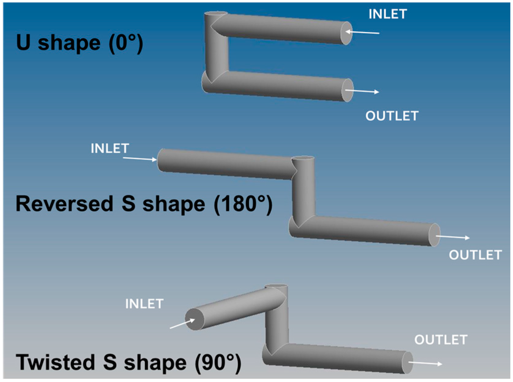
Here in the following we synthetized the results obtained from the CFD analysis of a path with two 90° bends (elbows); these test cases have been previously studied in literature. Hence we can compare the numerical results with the results published in papers and moreover with experimental results measured on our test rig. The geometries analyzed are shown in the following Figure 1. The channel diameter d is 6 mm and the maximum flow rate tested is 65 L/min, thus giving a correspondent maximum velocity value of about 38 m/s and maximum Reynolds number Re of about 5000.
The first geometry is the characteristic U shape: the two elbows are positioned adopting a twisting angle θ of 0°. The twisting angle is the angle swept out by the upper portion of the channel on a plane perpendicular to the figure plane. When the twisting angle is 90° the upper part of the channel is perpendicular to the figure plane, and the geometry appears as a twisted S, and when the twisting angle is 180° the upper channel is again on the plane of the figure, but the shape is similar to a reversed S. As already pointed out in the introduction, these geometries have been characterized in literature and our results can be compared with these ones, thus allowing also validating the numerical analysis.
Following the settings of the analysis performed in [2], where different single 90° bends were analyzed by means of a CFD analysis, the unstructured mesh has been designed in order to obtain a ratio between the element size and the minimum channel diameter equal to 0.06. This has been the best negotiation between the need to obtain numerical results independent from the mesh generation and computational time reasonably affordable. The numerical results were aligned with both literature and experimental test, and in correspondence of lower ratio values the pressure losses remained unchanged, being the discrepancy lower than the accuracy of the pressure losses measurement (0.0335 MPa). When analyzing a new geometry, as a first step in the mesh generation, we always have chosen the 0.06 ratio between the element size and the smallest diameter in the geometry and then we checked if the results calculated with lower ratio values were significantly different from the first one; the difference was always lower than the accuracy of the sensors used for experimental measurements, confirming that the mesh generated was a good compromise between the computational time and the accuracy of the results. This leads, for the double elbows geometry, to the number of elements and nodes reported in Table 1.
The unstructured mesh has been generated by the automatic mesh generator available in the commercial software used [13]. The mesh near the internal walls (boundary layer mesh) is structured, characterized by four layers with a layer factor of 1.2 (multiplying it by the local isotropic length scale for the surface, the layer height is determined) and setting an automatic function it is possible to manage the growth rate of the layers.
Again, as studied in [2], an opportune entry length was considered in order to have a fully developed flow at the entrance of the manifold block in the numerical analysis. An estimate of the entry length for different types of flow depends on the Reynolds number Re (ratio between the product of fluid velocity and channel diameter and the fluid kinematic viscosity) and the channel diameter d and is given by ~0.06·Re·d for laminar flow while it is approximated with different formulas for turbulent flow, in which the influence of Re number is weaker; in many pipes flow of practical engineering interest, the entrance effect are insignificant after a pipe length equal to 10·d [15].
Besides, the turbulence model used was k-ε model, which is a general purpose model, quite robust, not too much accurate, but that has shown to perform well for the purpose of the work as also shown in [2], where a comparison with other turbulence model available in the software has been performed.
The fluid in the simulations is an ISO VG 46 mineral oil (kinematic viscosity 46 cSt at 40 °C) and density of 860 kg/m3; it is the same fluid available in the test rig described in the following and used for the experimental analysis. The imposed boundary conditions were atmospheric pressure at the outlet of the system and a flow rate at the inlet. As a reference for the reader, the maximum flow rate considered in the numerical and experimental analysis was 65 L/min, the maximum pressure losses measured in the case of the double elboes geometries was around 3 MPa.
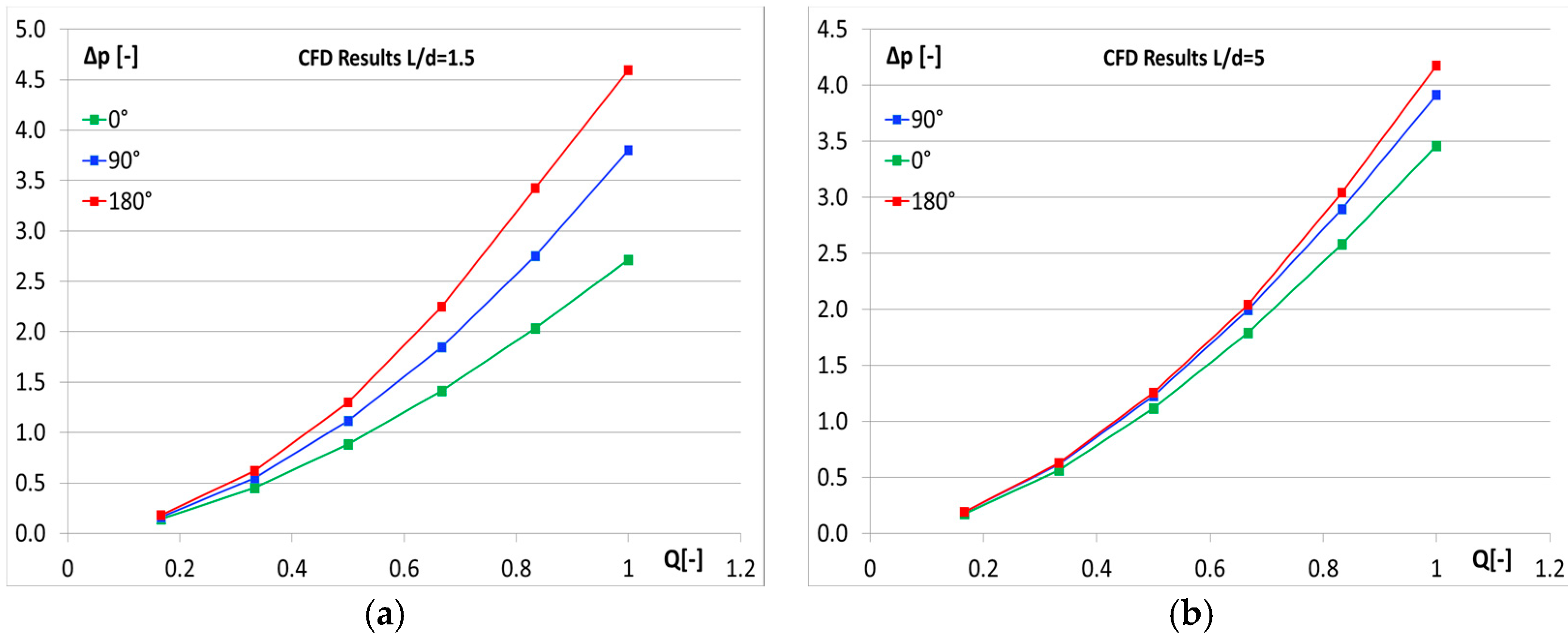
The first numerical result analyzed is the velocity field in the geometries simulated, to recover the results found in literature. In Figure 2 the velocity field is shown considering a distance L between the elbows of 5 times the channel diameter d; the three geometries are reported to highlight the differences. The velocity is non-dimensioned with respect to the inlet velocity value, which is 30 m/s for the test chosen. As also reported in [10], qualitatively speaking the flow deviation effect due to the first elbow is favorable for entering the second elbow in U geometry, while the flow path is more complex for the reversed S and even more troubled for the reversed S. The velocity field is strongly affected by the relative position of the two elbows: when the distance L between the elbows is less than 5∙d, the two elbows strongly influence each other and total pressure drops are very different to the one obtained by twice the loss on one elbow. In Figure 3 the pressure losses versus flow curves, obtained from CFD analysis, are shown for the three geometries considered and for two values of the distance between the elbows (1.5∙d and 5∙d). The pressure losses are non-dimensioned with respect to where ρ is the fluid density and v is the reference flow velocity defined as the maximum flow rate value used in the tests over the reference flow area at the inlet of the geometry considered.
The U geometry (0° twisting angle) shows that pressure losses increases as the two elbows are separated more (going form L/d = 1.5 to L/d = 5); the twisted S (90° twisting angle) has more or less the same losses when the mutual distance is modified, and finally the reversed S (180° twisting angle) shows decreasing losses with increasing mutual distance, and also the bigger ones among the three geometries. In [2] it was also shown that, when the mutual distance between the elbows is more than 10 times the channel diameters, the losses remain constant, that is the two elbows are independent one another. These total losses, as also observed in [10], are however lower than twice the loss of one elbow. In Figure 3 we can appreciate how the pressure losses for the three geometries are approaching one another when the distance is 5 times the channel diameter; this is a consequence of the fact that the elbows are further apart and their reciprocal orientation does not play a relevant role anymore on the total pressure loss.
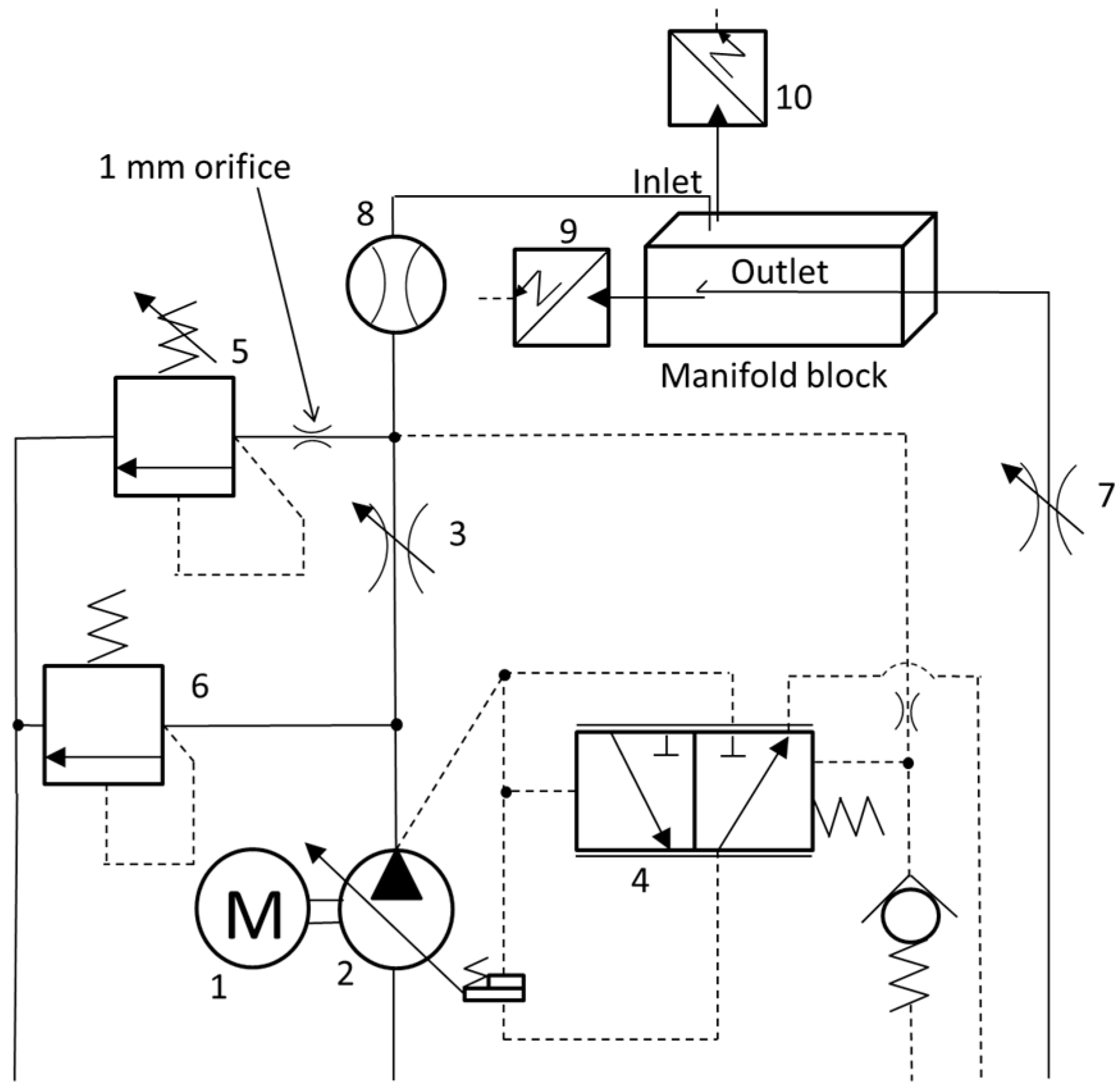
To validate the numerical analysis, a part from the comparison with the data found in literature, also an experimental analysis has been performed on a hydraulic manifold designed and manufactured for this purpose. The test rig is well described in [2] and here only the circuit layout (Figure 4) and the sensors characteristics together with the fluid properties are reported (Table 2 and Table 3) for completeness. During the tests we measured the pressure at the inlet and outlet sections of the manifold, using opportune pressure taps realized in the component, nearby the inlet and outlet of each geometry analyzed; the flow rate is measured at the inlet of the manifold. The fluid properties set in the numerical analysis were the same than the ones of Table 3. The accuracy of the measured pressure loss when measuring low pressure drops is quite low, due to the accuracy of the sensors, but progressively improves when measuring higher losses: the error in the experimental measurement of pressure drop of 0.1 MPa becomes 33.5%, at 0.5 MPa of pressure drop the error becomes 7%, at 1 MPa is about 3%. In the cases analyzed this means that for non-dimensioned pressure losses lower than 1 the experimental accuracy is very low, while it progressively improves for pressure losses higher than 1.
In Figure 5 the measured pressure losses on a manifold, opportunely designed with a dedicated CAD [16] and manufactured, are shown; still, the two distances L = 1.5∙d and L = 5∙d have been considered and the results are comparable to the numerical ones. It is established that at the higher distance of 5∙d, the measured losses are quite the same for the three geometries analyzed.
It is hence confirmed that two elbows may strongly interfere one another when their mutual distance is lower than five times the channel diameter; it is also within this distance that the geometry of the double elbow (U, twisted S or reversed S) can influence the pressure losses. Again, Figure 6 allows one to observe that, when the reciprocal distance between the two elbows is increasing, the differences in pressure losses for the three configuration considered are progressively reducing, both in numerical and experimental trends.
At the same time the discrepancy between the numerical and the experimental results increases when the reciprocal distance between the elbows is increasing, a statement already observed in [2]. These images have the aim to prove that the trends found in experimental test are the same of the numerical analysis, which is hence able to well depict the pressure losses trend. The results obtained from calculation are comparable to the diagrams published in [9,10].
3. Multiple Elbows
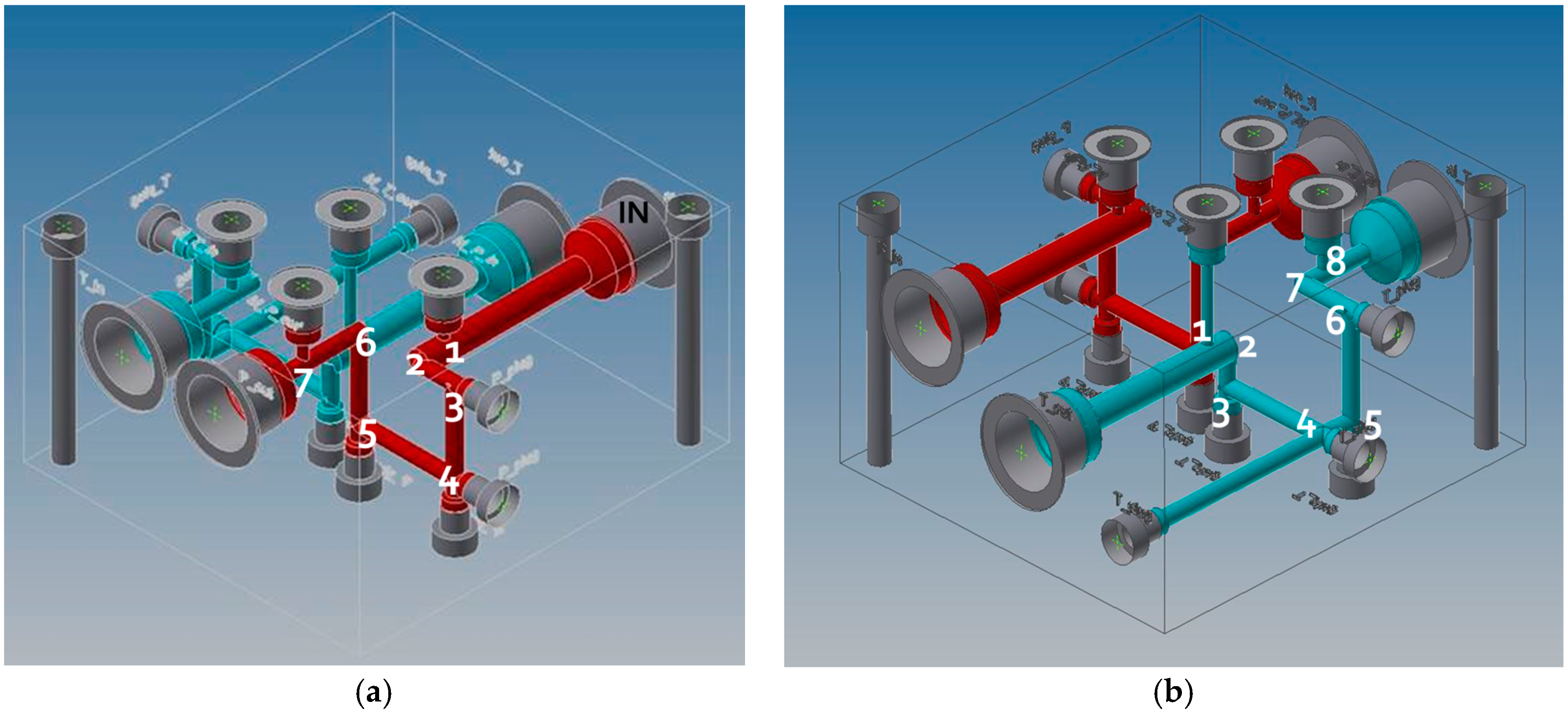
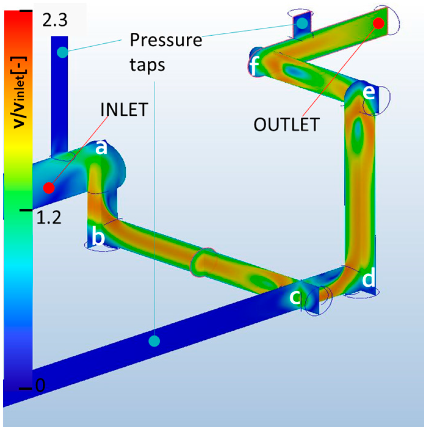
In real hydraulic manifolds the flow path may be much more complicated than a sequence of two elbows. In order to assess the quality of the numerical analysis, two different geometries, analyzed also in [11,12], were designed and manufactured. Also in these cases the numerical results were compared with the measured ones. The geometries are shown in Figure 7: in a unique manifold two paths have been realized, one with five 90° bends ((a) red) and one with six 90° bends ((b) light blue). At the inlet and outlet of the two paths there are opportune housings for the pressure sensors. The channel diameter d is 6 mm and the maximum flow rate tested is 65 L/min, thus giving a correspondent maximum velocity value of about 38 m/s and maximum Reynolds number Re of about 5000; the maximum pressure losses measured in this test case is nearly 6 MPa. In Table 4 the lengths of the straight portions of the two paths with reference to Figure 7 are listed. The numerical analysis has been performed adopting the settings described in the previous section and in Table 5. It has to be considered that, as reported in [9], the effect of a double elbow on the flow disappears after a distance that depends on the reciprocal orientation and space between the two elbows. For example, for a U shape with a reciprocal distance of almost five times the diameter of the channel, the effect disappears after a length equal to 50 times the channel diameter; if a twisted S shape is considered, with the same reciprocal distance between the elbows, this length becomes 80 times the channel diameters. The length values will remain the same or even increase if the reciprocal distance between the elbows is lower than five times the channel diameter.
It is clear from Table 4 that the distances in the internal paths considered are much shorter and this means that we cannot consider neither that each elbow is independent from the others nor can we discuss as if the elbows are coupled two by two and apply directly the considerations found for the double elbow test case. In this situation, hence, a correct evaluation of the total pressure losses can only come from the CFD analysis or the experimental analysis.
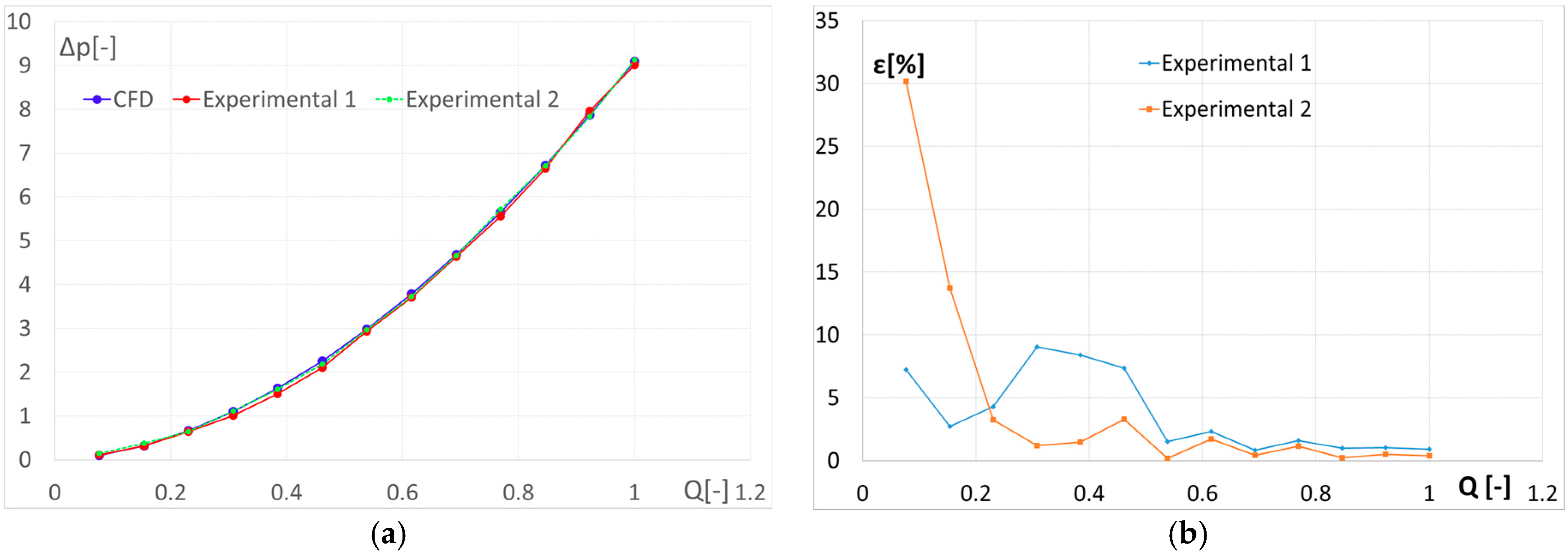
Results for the 5–90° bends path are reported below in Figure 8a, where the non-dimensioned pressure losses versus the non-dimensioned flow rate are shown; experimental tests, performed on a manifold designed and manufactured for the purpose, have been repeated (here below two tests are presented) and show good repeatability. Moreover, there is an excellent agreement between experimental and numerical results, also proved by the percentage differences ε reported in Figure 8b, calculated as the difference between the numerical and experimental pressure losses, relative to the experimental one. The highest value of ε is in correspondence of the lowest value of the pressure losses measured, when, however, the accuracy of the measurement is very low.
Results for the 6–90° bends path are reported below in Figure 9a, where the non-dimensioned pressure losses versus the non-dimensioned flow rate are shown. There is still an excellent agreement between experimental and numerical results, also proved by the percentage differences ε reported in Figure 9b.
The numerical analysis results have a very good agreement with the experimental ones when multiple elbows are considered, and this is due to the fact that the general purpose turbulence model chosen (the k-ε model) performs very well in these cases. When one elbow or two “distant” elbows are considered the distance between numerical and experimental results is higher as shown in [1]. However, as shown in [2], the CFD analysis is able to follow the trends of the pressure drops in each of the analyzed test cases. In the two paths concentrated pressure drop values in the elbows are different from each other according to the reciprocal orientation and distance of the elbows. The velocity field in the five elbows and six elbows paths is shown in Figure 10 and Figure 11. The velocity is non-dimensioned with respect to the inlet value; in particular, for the test shown in these figures this value is 30 m/s. Even if the six elbows path has one elbow more than the five elbows path, the pressure losses are more or less the same and this is again an evidence of the effect of the reciprocal influence of the elbows in a multiple elbows path. If the designer try to predict the overall loss as the sum of the individual ones obtained on each elbow, the result will overestimate much the real total loss for the entire path. Considering that each pressure loss can be determined as in Equation (1), according to [9], where:
- σ1 is the local coefficient of pressure loss on one elbow: Idelchik in [9] defined some tables that allow to determine three coefficients, (a, b, c) whose product give this term; a depends on the bend angle, b depends on the ratio between the radius of the rounded edges of the connection and the channel diameter, c is 1 in the case of a circular section.
- σr is the friction loss coefficient, which depends on the friction factor (determined using the Moody diagram or an analytical formulation as the Blasius formulation), on the ratio between the radius of the rounded edges of the connection and the channel diameter, on the bend angle; the total non-dimensioned pressure losses would be almost 13 for the 5-elbows path and almost 16 for the 6-elbows path at the maximum non-dimensioned flow rate of 1.
4. Inclined Connections or V-Bends
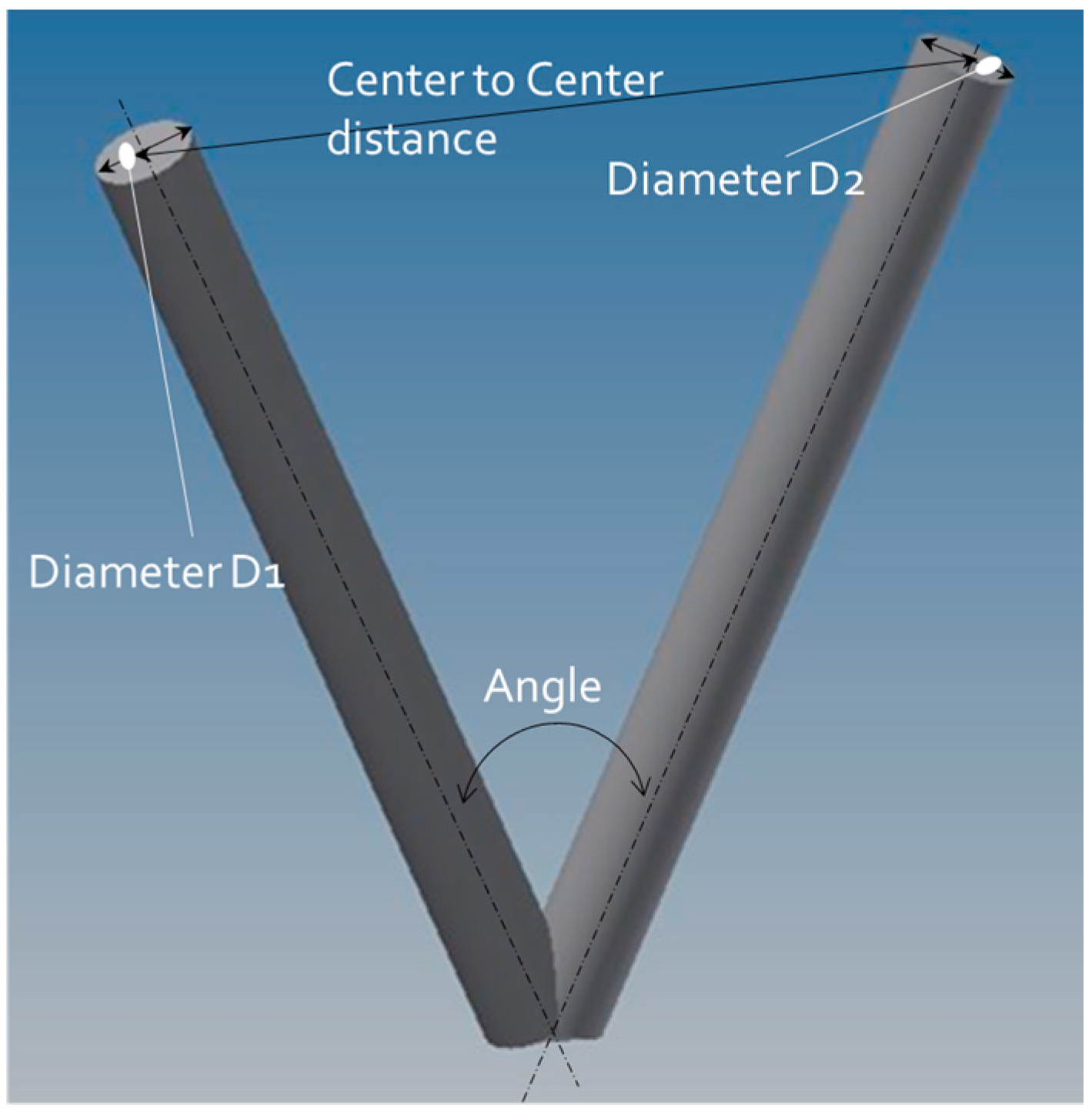
Although the designer will always prefer to realize connections in a manifold through straight channels, it is possible or in some cases mandatory, due to space reasons, to use inclined connections to join two cavities, realizing a V-bend. In this section we present the results coming from the CFD analysis applied to the study of the flow field inside this connection and the pressure losses, with the aim to highlight the influence of the main design parameters. In Figure 12 an example of this kind of connection is shown, where the main geometrical parameters considered are pointed out. In addition to the angle between the channels and the “center to center distance”, we considered different flow rate conditions (or corresponding flow velocity values) and different values of viscosity for the fluid. The diameter of the channels is 10 mm.
In order to analyze the effect of all these parameters it was chosen to develop a Design of Experiment (DOE) analysis: an “experimental” plan of 324 simulations has been designed, to cover at least three levels of variation for the kinematic viscosity and “center to center distance”, four levels for the reference fluid velocity (that correspond to four levels of flow rate) and nine levels for the angle between the channels (Table 6). We have chosen to introduce many levels for the angle because we expected that the trend of the pressure losses versus the angle is the most critical to be depicted. In this analysis the diameters of the two channels were kept the same (D1 = D2 = D) and equal to 10 mm. We have performed all the numerical simulations to determine the pressure losses through CFD analysis, with the mesh characteristics shown in Table 7. Then, we have used Minitab [17], commercial software used for statistical analysis of data, to analyze the interaction among the factors.
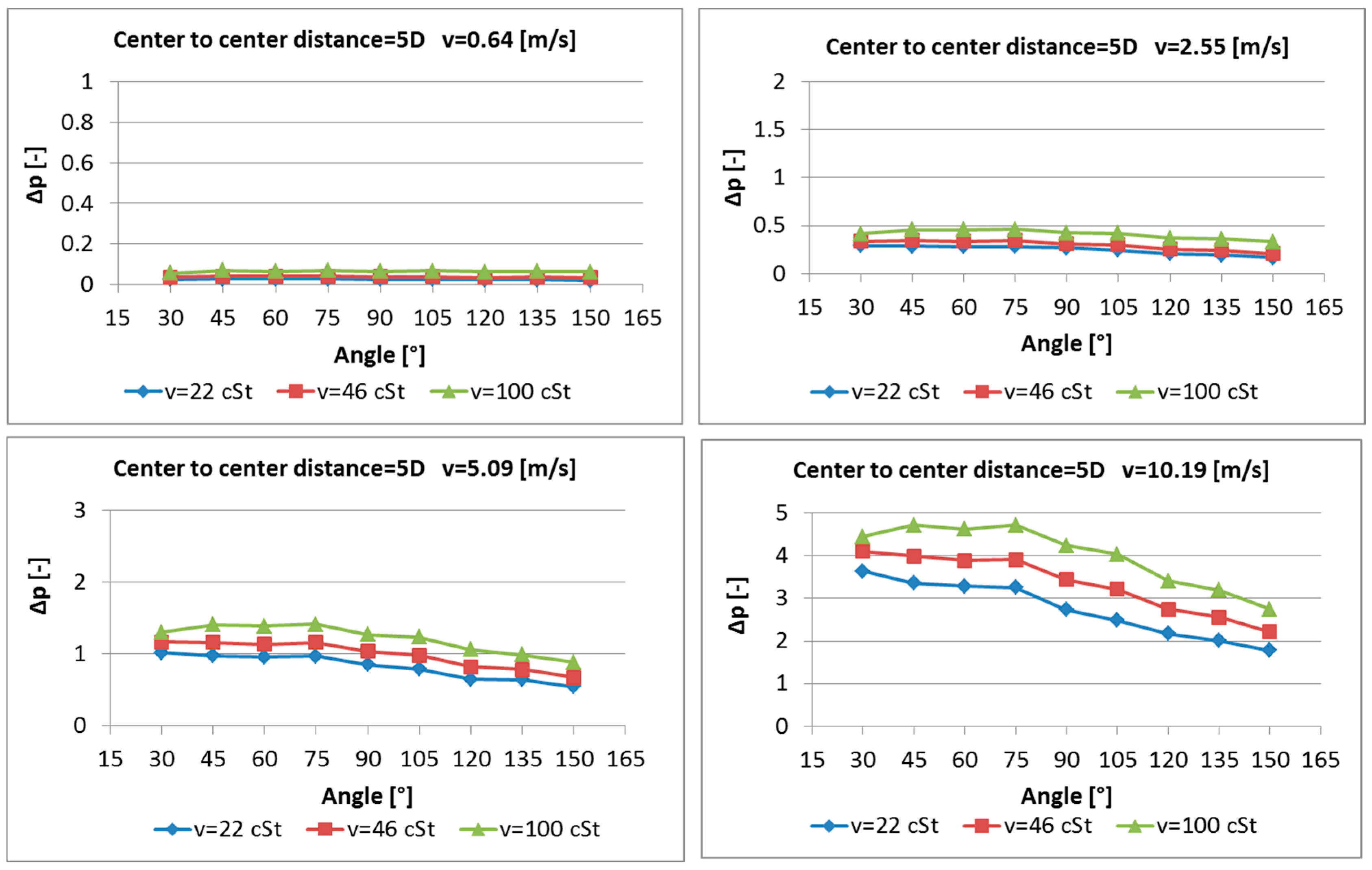
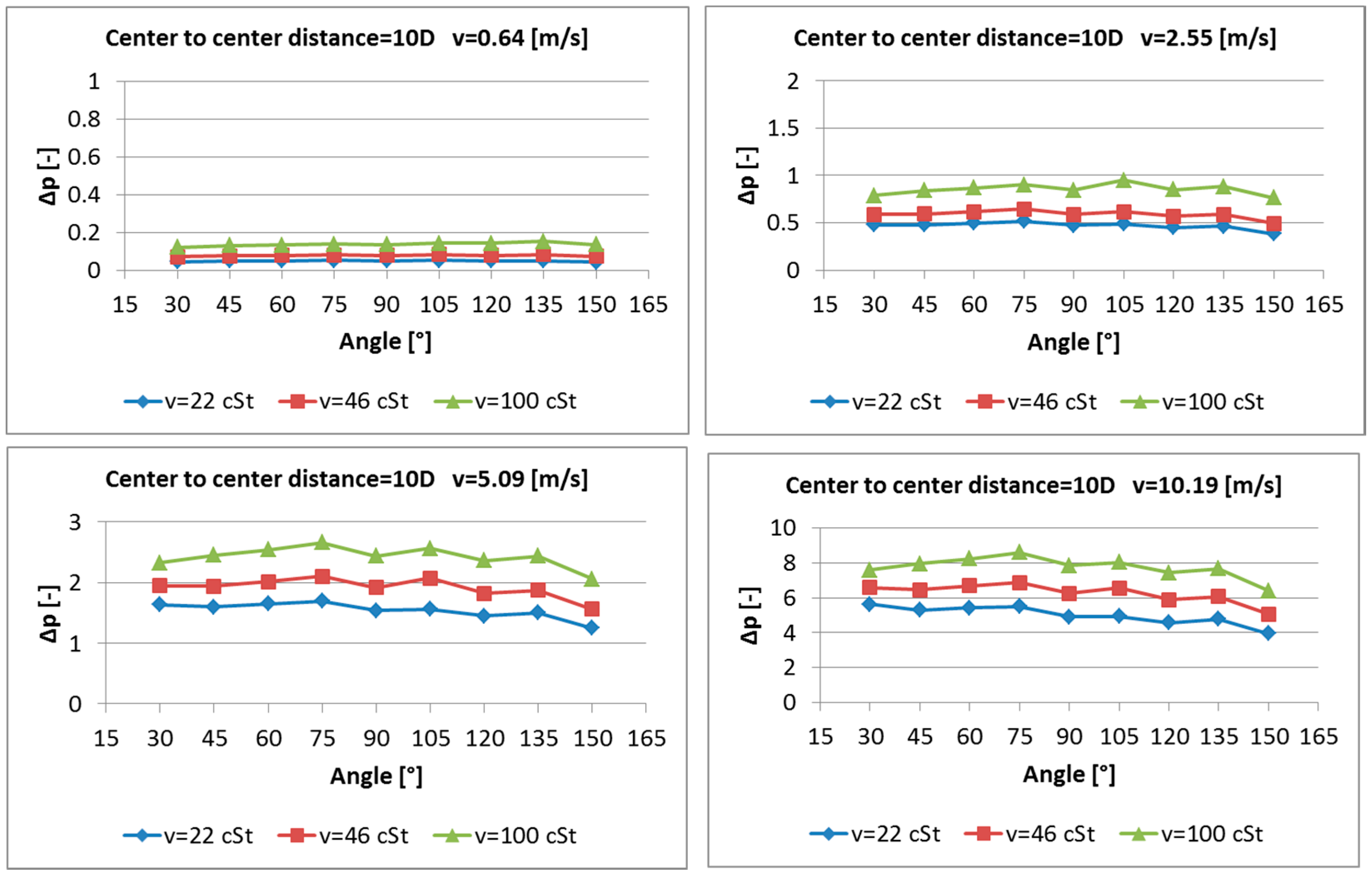
In Figure 13 the results in terms of non-dimensioned pressure losses are reported as function of the angle, for the three levels of viscosity and for a “center to center distance” equal to 3∙D; moreover each graph correspond to a different value of flow velocity. In a similar way, Figure 14 shows the pressure losses for the “center to center distance” of 5∙D and Figure 15 shows the pressure losses for the “center to center distance” equal to 10∙D. The pressure losses are still non-dimensioned with respect to where ρ is the fluid density and v is the reference flow velocity defined as the maximum flow rate in the tests performed over the flow area at the inlet of the geometry considered. As a reference for the reader the maximum pressure losses is here 0.4 MPa.
From the images above, it is evident that the pressure losses increase with the reference fluid velocity (i.e., the inlet flow rate) and with the fluid viscosity, as expected; they grow with the “center to center distance”, and this is also expected because, with the same angle and an higher distance, the straight part of the channels are longer and introduce more losses.
Pressure losses have, instead, a peculiar trend with angle: it is evident that at 75° there is a change in the trend of pressure losses. At a “center to center distance” of 3∙D and 5∙D, the pressure loss is almost constant with the angle going from 30° to 75° while it decreases more consistently from 75° to 150° angle values. For a “center to center distance” of 10∙D the pressure loss slightly increases with the angle going from 30° to 75° while it decreases with an unstable trend from 75° to 150° angle values. However, we can say that, if a V-bend has to be considered, once the angle is lower than 90°, whatever value it assumes, it does influence weakly the pressure losses, which have reached almost their highest values.
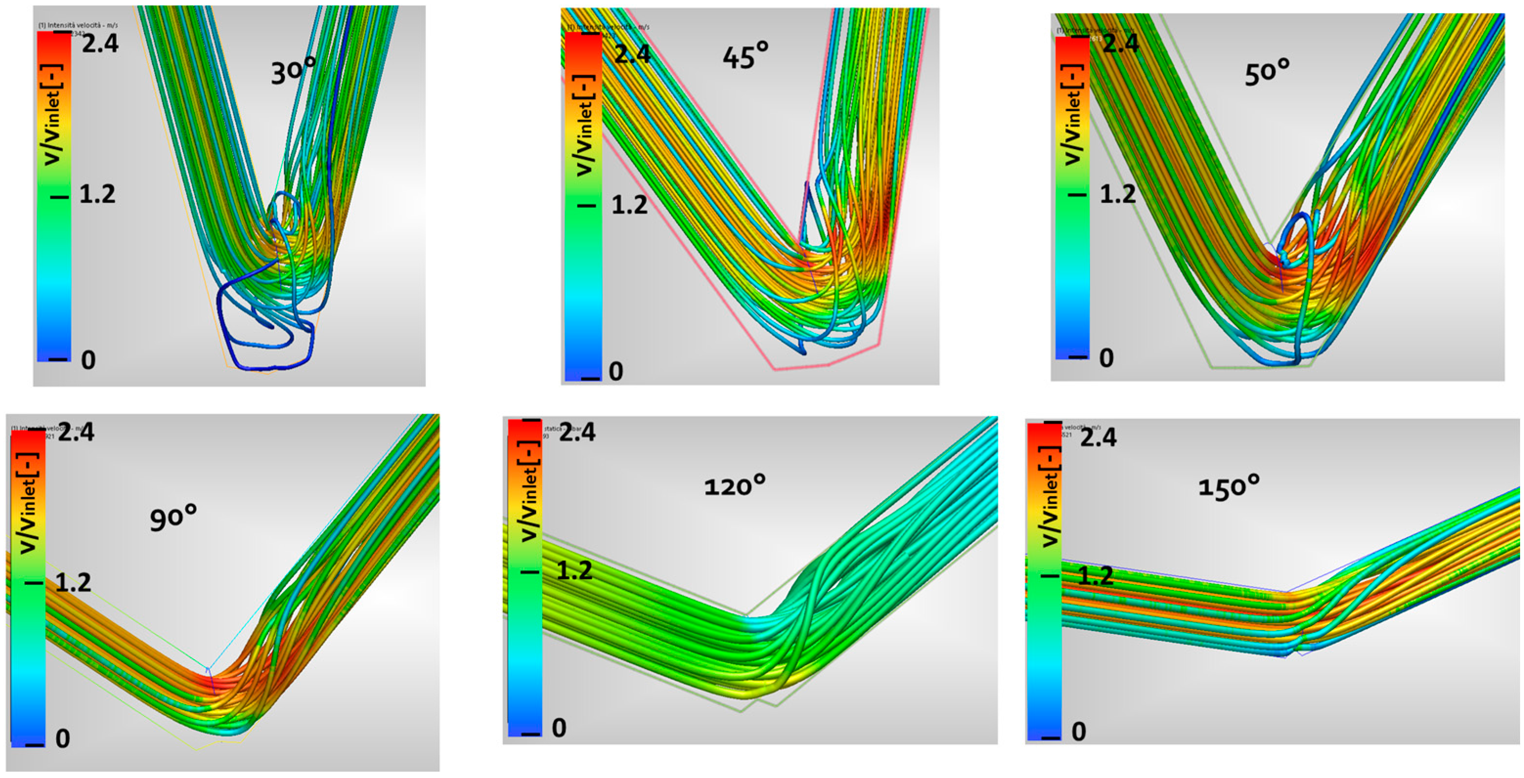
In Figure 16 and Figure 17 respectively, the non-dimensioned velocity intensity map and the streamlines are shown, for the fluid reference velocity of 2.55 m/s (12 L/min), kinematic viscosity of 15 cSt and a “center to center distance” equal to 10∙D. The inlet of fluid is in the left channel, the outlet in the right channel. It can be seen how the flow detaches from the wall just after the bend and this causes a strong swirl around the channel axes, until the angle increases well over the 90° value. Streamlines show better that there is a strong swirling action of the flow when the angle is lower than 90°.
We used these data coming from numerical simulations to analyze the effect of the parameters characterizing the V-bend on the pressure losses and their eventual interaction. Before drawing conclusions about the effects of the factors and the interactions among them, it is necessary to check the three assumptions of ANOVA analysis (ANalysis Of VAriance): normality, constant variance and independence.
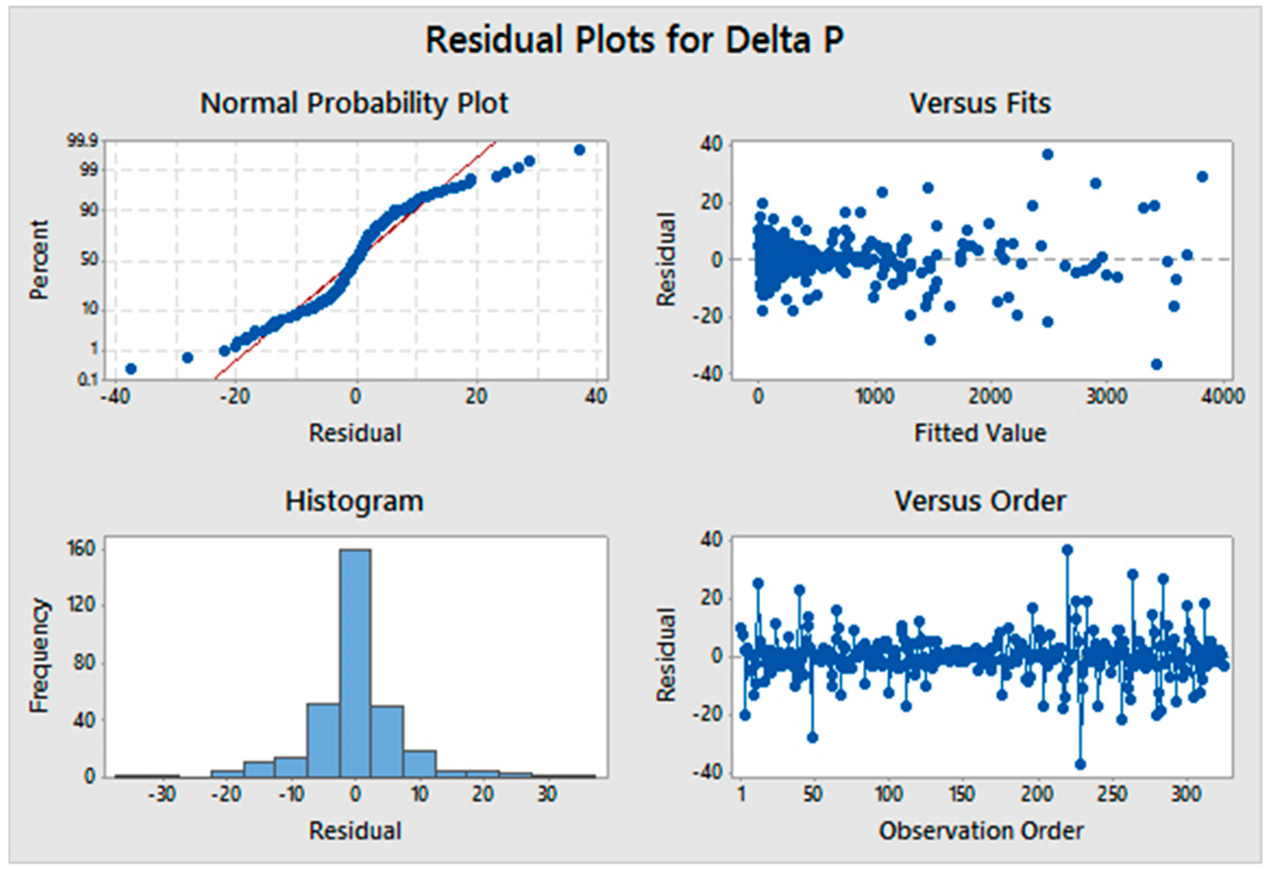
The residual is the difference between a pressure loss value calculated with CFD and its corresponding fitted value. A residual plot is a graph that is used to examine the goodness-of-fit in regression and ANOVA. Examining residual plots helps to determine whether the ordinary least squares assumptions are being met. If these assumptions are satisfied, then ordinary least squares regression will produce unbiased coefficients estimates with the minimum variance.
In the normal probability plot the points should form a straight line if the residuals are normally distributed. The plot of residuals versus fitted values should show a random pattern on both sides of zero if the assumption of linear relationship is reasonable and the residuals should form a ‘horizontal band’ centered in the horizontal axes (line at zero residual) if the assumption of constant variance is reasonable. Histogram of residuals is another proof of the normal distribution of residuals: normally distributed data, by definition, exhibit relatively little skewness. Residuals versus order is a plot of all residuals in the order the data was collected and helps to check the assumption that the residuals are uncorrelated with each other. In this case the data do not come from experimental tests but from CFD analysis, so there cannot be non-random errors due to time-related effects. In our analysis the normality plot and the histogram show that the residuals follow a normal distribution; both plot of residuals versus fitted values and versus run order do not show any pattern, thus constant variance and independence assumptions are satisfied (Figure 18). ANOVA assumptions are checked and we can trust the following considerations as statistically significant, with a level of confidence of 95%.
The “Main Effects Plots” for the pressure losses are shown in Figure 19; in this figure if the line showing the results is quite flat, it means that the values of pressure loss, obtained varying the factor between the lower level and higher level, are nearby the mean value, that is the variation of that factor has a small influence on the pressure losses establishing. From the plots in Figure 19 it is shown that the variation of the angle has little influence on the pressure loss—especially when the angle is lower than 90°—, as well as the variation of the kinematic viscosity in the interval considered; the variation of “center to center distance” has a stronger effect on pressure losses and the variation of the fluid velocity has the strongest influence as it is expected.
The “Interaction plots” in Figure 20 compare the combined effect of two factors at a time: for example, in the first plot “Center-Center × Angle”, the trend of the pressure losses is observed for each curve varying the “center to center distance” reported on the x-axes and each of the 9 lines reported in the plot corresponds to a value of angle. For each plot, the first factor is varying on the x-axes, while each line corresponds to a value of the second factor considered. If there is intersection between the curves, there is also interaction between the two factors considered; if the lines are almost parallel there is no interaction between the two factors. The absence of interactions between the lines in the “Interaction Plot” reported in Figure 20 shows that there are no interactions between the four factors, in the range of variation considered: center-to-center distance, angle, velocity and kinematic viscosity have all an influence, more or less strong, in the pressure losses establishing but their effect on the pressure losses is independent one another. This means that, if we imagine a pressure drop curve as function of one of the parameters, we can use different combinations of all the other parameters and the trend will remain the same. This result justifies the eventual creation of a predictive function for the pressure losses for the V-bends, obtained from the numerical data fitting.
To conclude the analysis of the V-bends, we now introduce expansion/contraction geometry to assess if the general considerations depicted in [2] for a 90° bend are still valid in these cases. We considered for this analysis only one value of the fluid velocity, 6.4 m/s; the pressure losses are non-dimensioned with respect to the maximum fluid velocity analyzed in this paragraph, 10.2 m/s, to allow adequate comparison with the previous data. The other characteristic data are reported in Table 8. We considered an expansion/contraction ratio which is the ratio between the higher diameter considered and the smaller one.
In the expansion diagram (Figure 21a) the pressure losses decrease strongly with the expansion ratio going from 1 to 1.4, for all the values of angle considered, and then remain almost constant. At expansion ratio equal to 1, the pressure losses of the V-bend at 30°, 60°, 90° and 120° are similar, while at 150° the loss is lower; when the expansion ratio rises the pressure losses remain very comparable, the effect of the angle is mixed with the effect of the expansion and it is not possible to define a clear influence of the angle anymore. In Figure 22 the velocity intensity map are shown for an expansion ratio of 2 and a reference fluid velocity of 6.4 m/s (flow rate 30 L/min); the velocity is non-dimensioned with respect to this reference value. The inlet of fluid is still in the left channel, the outlet in the right channel. For angle values lower than 90°, the flow impacts the wall entering in the bigger channel and then is accelerated towards the bigger channel exit. For 120° and 150° the flow is more easily directed to the bigger channel.
In the contraction diagram (Figure 21b), again the pressure losses decrease considering a contraction ratio going from 1 to 1.4 and then remain almost the same. The decrease trend is, however, much less drastic in this case compared to the previous one. This suggests that, if a V-bend has to be introduced in the manifold, a slight expansion helps reducing the pressure losses, and the contraction does not introduce additional pressure losses.
Finally, in Figure 23 the velocity intensity map are shown for a contraction ratio of 2 and still a reference fluid velocity of 6.4 m/s (flow rate 30 L/min); the velocity is non-dimensioned with respect to this reference value. For angle values lower than 90°, the flow detaches from the wall in the inner part of the smaller channel, while for higher angles the flow detaches at the outer wall of the smaller channel.
5. Conclusions
This work has been focused on the study of pressure losses on manifolds, with the aim of deepening some aspects which have not been considered in a previous work on the topic [2] and for which the scientific literature in the field of fluid power applications is quite poor, as far as the authors know.
The study has been performed using CFD analysis with a commercial software and experimental analysis for the first two test cases considered, the double elbows geometry and the multiple elbows geometry.
The double elbows test case, also presented in [2], has been used here to explain the settings and characteristics of the numerical analysis, i.e., the mesh generation, the choice on the turbulent model and the boundary conditions. Some results not shown in the previous paper have been presented, which allow analysing the influence of the reciprocal orientation of the elbows and their distance. As found also in literature, it has been shown that when the two elbows form a U geometry the pressure losses are considerably lower than in the other cases (reversed or twisted S shape), that when the reciprocal distance between the elbows becomes higher than five times the channels diameter, the elbows are less influencing one another and that when this distance is higher than 13 times the channel diameter the elbows are not influencing one another anymore. In this last case, the total pressure loss value is near twice the loss on a single elbow. Moreover, the designer has to keep in mind that the best configuration for pressure loss reducing in the manifold is not to keep a great distance between the elbows, but instead to maintain a reciprocal distance less than 5 times the diameter and introducing a U shape or, if a U shape is not possible, to avoid geometries in which the twisting angle θ between the pipe channels is between 90° and 180°.
After that, more complex and realistic paths involving multiple elbows with variable reciprocal orientation and distances have been introduced, that have not been studied in previous paper [2]; to assess the ability of the CFD analysis to well depict the pressure losses trends in this case, we have chosen to replicate two geometries found in literature ([12,13]) and to perform both a numerical analysis and an experimental analysis after having designed and realized an opportune manifold. The results display a very good agreement between the numerical and the measured data, showing that the k-ε turbulent model performs very well even if it is considered normally not too much accurate. The results obtained also highlight how the designer should not optimize a geometry on the basis of the pressure loss calculated as the sum of the pressure losses on each elbow; this method in fact would lead to overestimate too much the pressure losses if the elbows are sufficiently near one another and does not consider at all the elbows reciprocal position.
After having shown that the numerical results are coherent with the measured ones in the previous tests, the CFD analysis has been used to study a particular geometry, the V-bend, which can be realized in a manifold because of the lack of space and the presence of multiple connections. This geometry has not been studied in [2], nor can we find data regarding the pressure losses for hydraulic manifolds in literature. The simulation has allowed to test different geometries obtained changing the main geometrical parameters characterizing the V-bend and the fluid flow and viscosity. A plan of numerical simulations has been realized and the results have been shown with reference to each parameter considered: it was shown that the variation of flow rate (fluid velocity) and “center to center distance” between the channels affect more the pressure losses trend, which increases with these two factors. On the other hand, the variation of the angle of the V connection seems to have a smaller influence. We have seen that, in the angle range analysed, from 30° to 75°, the pressure losses are more or less constant and at their higher values; if the angle is increased more, the pressure losses progressively decrease. For these reason, as a suggestion, the designer has to avoid the use of V connections with angle lower than 90°, while angles higher than this value in any case causes pressure loss values lower than the 90° bend. Having shown the independence of the influence of each parameter on the pressure losses trend, it is suggested that an empirical function can be defined on the basis of the calculated data and successively used to predict the pressure losses in different conditions, moving into the range of variation of the parameters considered.
Finally, the pressure losses on the V-bend have been analysed also considering an expansion/contraction ratio between the diameters of the channels; the analysis confirms that, as for the 90° bend studied in [2], the expansion helps to lower the pressure losses; the contraction shows a much more slight decrease of the losses. However, this suggests that if a V-bend has to be introduced in the manifold, a slight expansion helps reducing the pressure losses, and the contraction does not introduce additional pressure losses.
Acknowledgments
The authors want to kindly acknowledge VEST Inc. and Pintotecno for the support of the research.
Author Contributions
Barbara Zardin, Giovanni Cillo, conceived, designed and realized the experiments and numerical analysis, Alessandro D’Adamo helped in the numerical analysis; Barbara Zardin, Giovanni Cillo, Alessandro D’Adamo and Massimo Borghi analyzed the data; Barbara Zardin, Giovanni Cillo and Massimo Borghi wrote the paper, Alessandro D’Adamo and Stefano Fontanesi revised it.
Conflicts of Interest
The authors declare no conflict of interest.
References
- Borghi, M.; Zardin, B.; Pintore, F.; Belluzzi, F. Energy Savings in the Hydraulic Circuit of Agricultural Tractors. Energy Procedia 2014, 45, 352–361. [Google Scholar] [CrossRef]
- Zardin, B.; Cillo, G.; Rinaldini, C.A.; Mattarelli, E.; Borghi, M. Pressure Losses in Hydraulic Manifolds. Energies 2017, 10, 310. [Google Scholar] [CrossRef]
- Love, L.J.; Lanke, E.; Alles, P. Estimating the Impact (Energy, Emissions and Economics) of the U.S. Fluid. Available online: http://www.osti.gov/scitech/biblio/1061537-estimating-impact-energy-emissions-economics-us-fluid-power-industry (accessed on 5 June 2017).
- Martinopoulos, G.; Missirlis, D.; Tsilingiridis, G.; Yakinthos, K.; Kyriakis, N. CFD Modeling of A Polymer Solar Collector. Renew. Energy 2010, 35, 1499–1508. [Google Scholar] [CrossRef]
- Verstraete, T.; Coletti, F.; Bulle, J.; Vanderwielen, T.; Arts, T. Optimization of a U-Bend for Minimal Pressure Loss in Internal Cooling Channels—Part I: Numerical Method. ASME J. Turbomach. 2013, 135, 051015. [Google Scholar] [CrossRef]
- Coletti, F.; Verstraete, T.; Bulle, J.; Van der Wielen, T.; Van den Berge, N.; Arts, T. Optimization of a U-Bend for Minimal Pressure Loss in Internal Cooling Channels—Part II: Experimental Validation. ASME J. Turbomach. 2013, 135, 051016. [Google Scholar] [CrossRef]
- Serre, M.; Odgaard, A.J.; Elder, R.A. Energy Loss at Combining Pipe Junction. J. Hydraul. Eng. 1994, 120, 808–830. [Google Scholar] [CrossRef]
- Štigler, J.; Klas, R.; Kotek, M.; Kopecký, V. The Fluid Flow in the T-Junction. The Comparison of the Numerical Modeling and Piv Measurement. Procedia Eng. 2012, 39, 19–27. [Google Scholar] [CrossRef]
- Idelchik, I.E. Handbook of Hydraulic Resistance, 2nd ed.; Hemisphere Publishing Co.: Washington, DC, USA, 1986. [Google Scholar]
- Murakami, M.; Shimizu, Y.; Shiragami, H. Studies on fluid flow in three-dimensional bend conduits. Bull. JSME 1969, 12, 1369–1379. [Google Scholar] [CrossRef]
- Abe, O.; Tsukiji, T.; Hara, T.; Yasunaga, K. Pressure drop of pipe flow in manifold block. In Proceedings of the 8th JFPS International Symposium on Fluid Power, Okinawa, Japan, 25–28 October 2011. [Google Scholar]
- Abe, O.; Tsukiji, T.; Hara, T.; Yasunaga, K. Flow analysis in pipe of a manifold block. IJAT 2012, 6, 494–501. [Google Scholar] [CrossRef]
- Autodesk® Simulation CFD 2013 Manual, Autodesk. Available online: https://knowledge.autodesk.com/support/cfd/downloads (accessed on 5 June 2017).
- Wang, J. Theory of flow distribution in manifolds. Chem. Eng. J. 2011, 168, 1331–1345. [Google Scholar] [CrossRef]
- Merritt, H.E. Hydraulic Control Systems; John Wiley & Sons: Chichester, UK, 1967. [Google Scholar]
- MDTools® 750 Manual, VEST Inc. Available online: http://www.vestusa.com/Download/MDTools-750-User-Manual.pdf (accessed on 5 June 2017).
- Minitab. Available online: https://www.minitab.com/en-us/support/documentation/ (accessed on 5 June 2017).
Figure 1.
Double elbows geometries analyzed.

Figure 2.
Velocity intensity map for the three double elbows geometries considered and a reciprocal distance between the elbow of 5·D.
Figure 2.
Velocity intensity map for the three double elbows geometries considered and a reciprocal distance between the elbow of 5·D.

Figure 3.
Numerical non-dimensioned pressure losses for the three geometries analyzed and for two values of the reciprocal distance between the elbows. (a) L/d = 1.5; (b) L/d = 5
Figure 3.
Numerical non-dimensioned pressure losses for the three geometries analyzed and for two values of the reciprocal distance between the elbows. (a) L/d = 1.5; (b) L/d = 5

Figure 4.
Circuit layout diagram of the test rig.

Figure 5.
Measured non-dimensioned pressure losses for the three double elbows geometry considered and for two values of the reciprocal distance between the elbows. (a) L/d = 1.5; (b) L/d = 5.
Figure 5.
Measured non-dimensioned pressure losses for the three double elbows geometry considered and for two values of the reciprocal distance between the elbows. (a) L/d = 1.5; (b) L/d = 5.

Figure 6.
Measured non-dimensioned pressure losses for the three double elbows geometry considered and for three values of the reciprocal distance between the elbows. (a) L/d = 1.5; (b) L/d = 5; (c) L/d = 13.
Figure 6.
Measured non-dimensioned pressure losses for the three double elbows geometry considered and for three values of the reciprocal distance between the elbows. (a) L/d = 1.5; (b) L/d = 5; (c) L/d = 13.
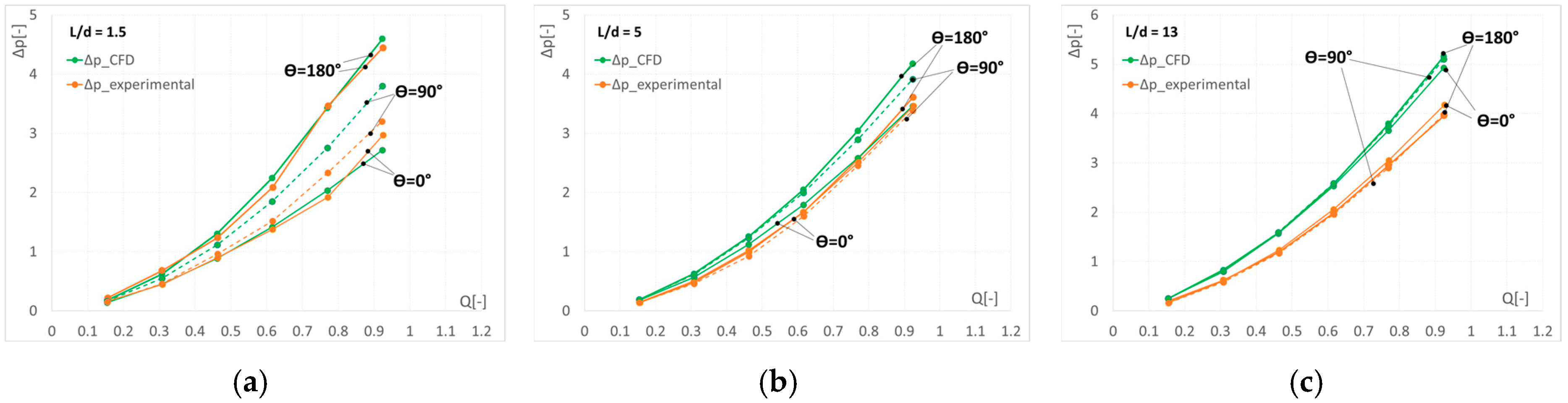
Figure 7.
CAD image of the manifold with the two paths: five 90° bends ((a) red); six 90° bends ((b) light blue).
Figure 7.
CAD image of the manifold with the two paths: five 90° bends ((a) red); six 90° bends ((b) light blue).

Figure 8.
Experimental and numerical non-dimensioned pressure losses (a) and relative difference for the two experimental test cases performed (b).
Figure 8.
Experimental and numerical non-dimensioned pressure losses (a) and relative difference for the two experimental test cases performed (b).

Figure 9.
Experimental and numerical non-dimensioned pressure losses (a) and relative difference for the two experimental test cases performed (b).
Figure 9.
Experimental and numerical non-dimensioned pressure losses (a) and relative difference for the two experimental test cases performed (b).
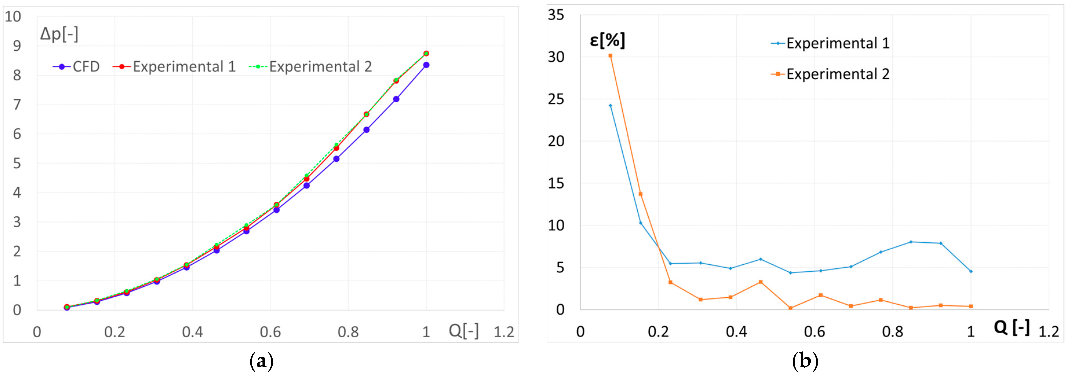
Figure 10.
Velocity intensity map for the 5-elbows path.
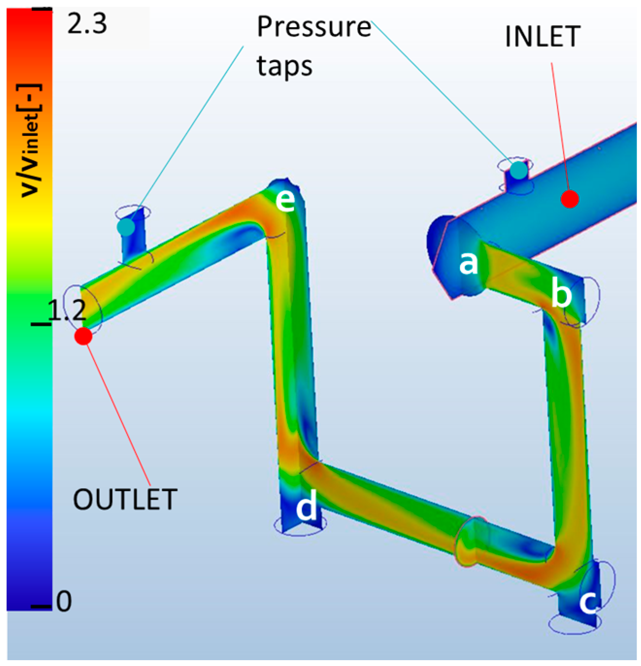
Figure 11.
Velocity intensity map on the 6-elbows path.

Figure 12.
V-bend and geometrical parameters (factors) considered in the analysis.

Figure 13.
Non-dimensioned pressure losses for the “center to center distance” of 3∙D.
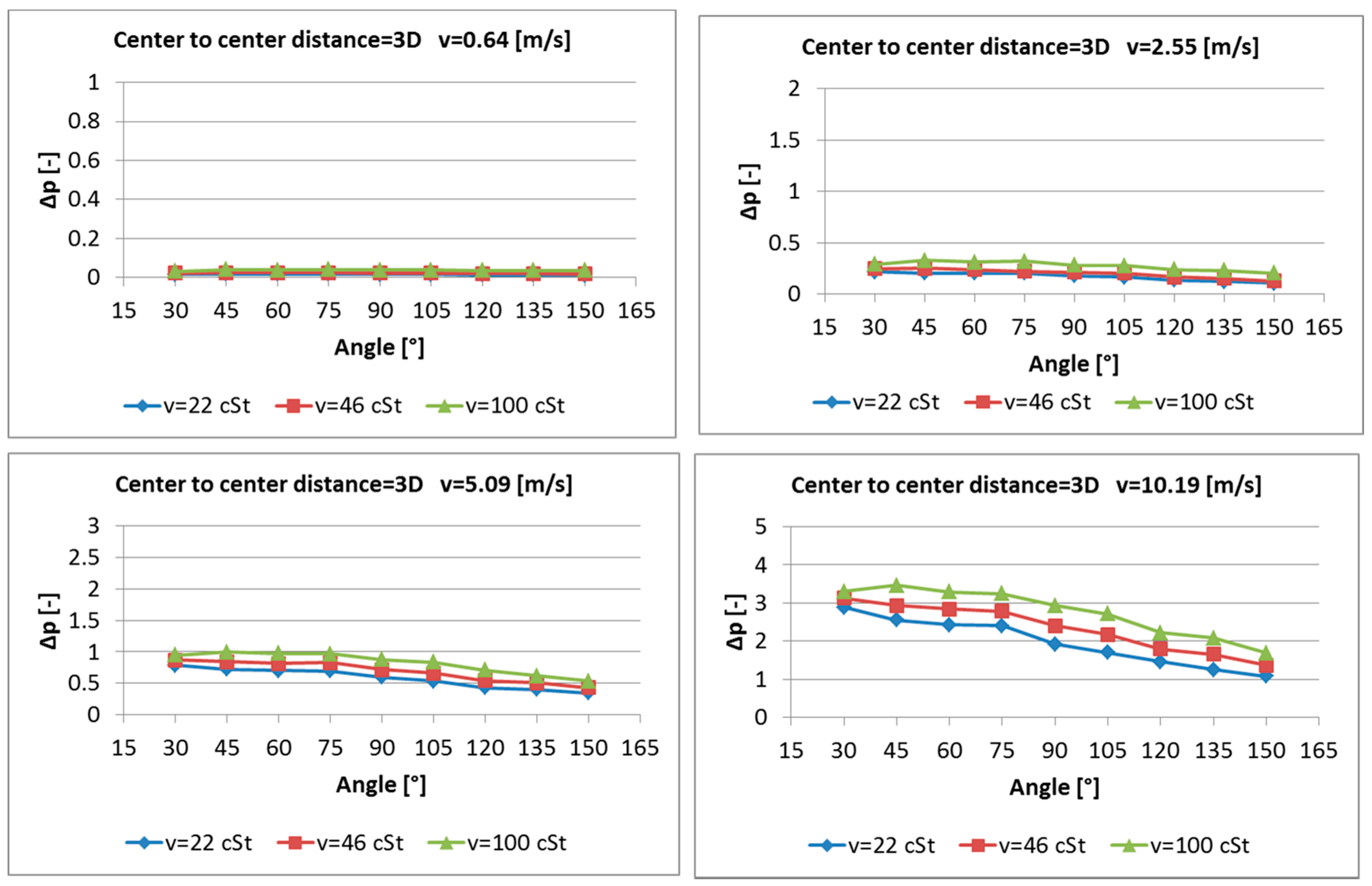
Figure 14.
Non-dimensioned pressure losses for the “center to center distance” of 5∙D.

Figure 15.
Non-dimensioned pressure losses for the “center to center distance” of 10∙D.

Figure 16.
Fluid velocity intensity map for different angle of the connection; reference fluid velocity 2.55 m/s (inlet flow rate 12 L/min), 15 cSt, “center to center distance” of 10·D.
Figure 16.
Fluid velocity intensity map for different angle of the connection; reference fluid velocity 2.55 m/s (inlet flow rate 12 L/min), 15 cSt, “center to center distance” of 10·D.

Figure 17.
Stream lines for different angle of the connection; reference fluid velocity 2.55 m/s (inlet flow rate 12 L/min), 15 cSt, “center to center distance” of 10·D.
Figure 17.
Stream lines for different angle of the connection; reference fluid velocity 2.55 m/s (inlet flow rate 12 L/min), 15 cSt, “center to center distance” of 10·D.

Figure 18.
Plot of the residuals of the pressure losses calculated in the 324 simulations performed.
Figure 18.
Plot of the residuals of the pressure losses calculated in the 324 simulations performed.

Figure 19.
Effects of the factors analyzed (“center to center distance”, angle, viscosity, fluid reference velocity) on the non-dimensioned pressure losses.
Figure 19.
Effects of the factors analyzed (“center to center distance”, angle, viscosity, fluid reference velocity) on the non-dimensioned pressure losses.
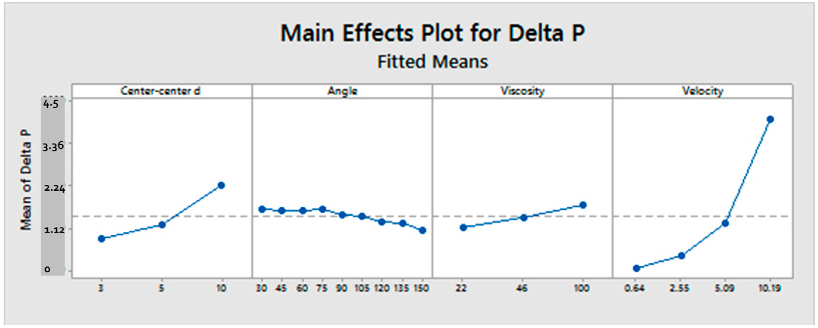
Figure 20.
Interaction plot for the non-dimensioned pressure losses in the inclined connection.
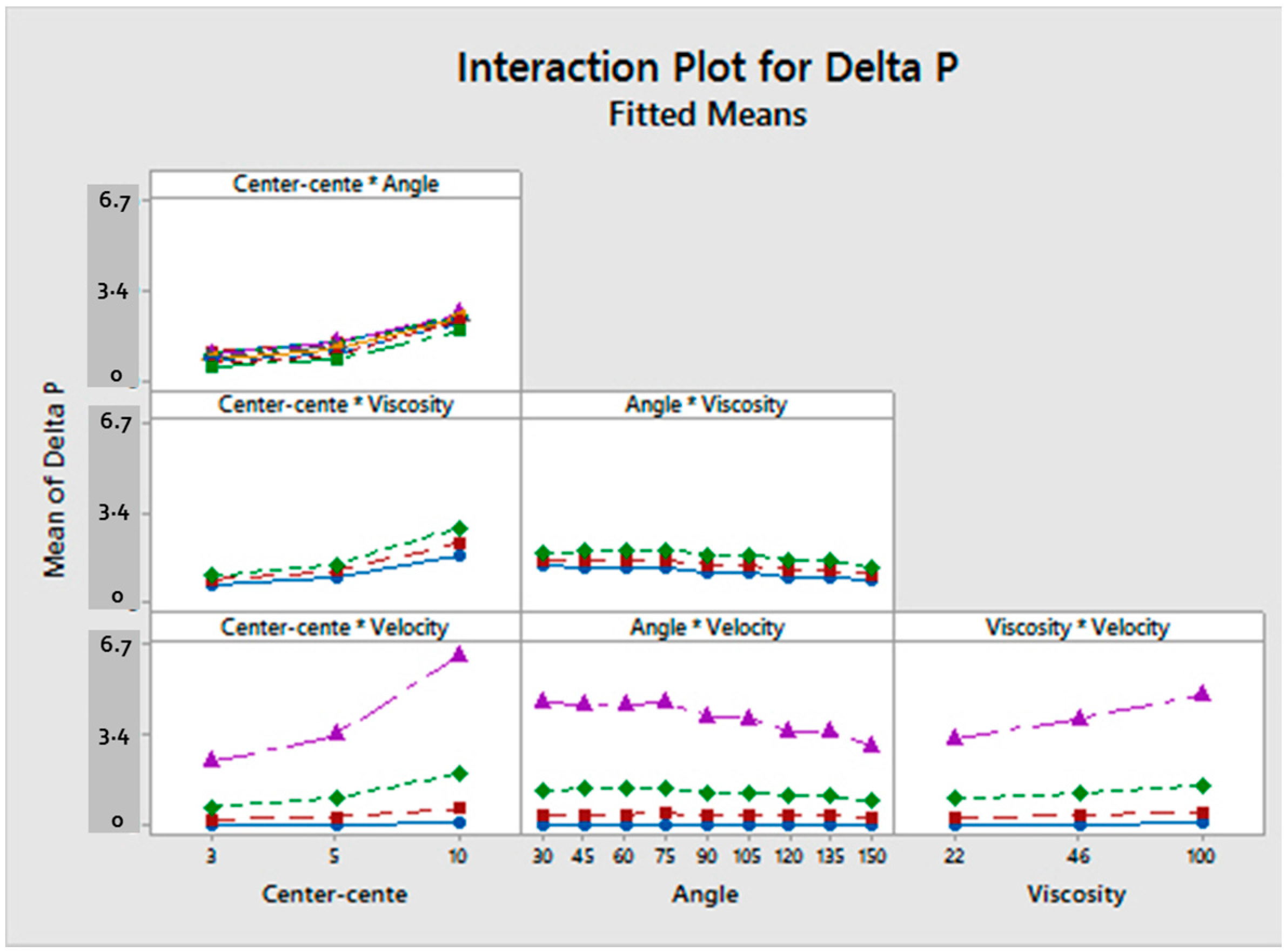
Figure 21.
Non-dimensioned pressure losses versus the expansion (a) and contraction ratio (b), for different angle values.
Figure 21.
Non-dimensioned pressure losses versus the expansion (a) and contraction ratio (b), for different angle values.
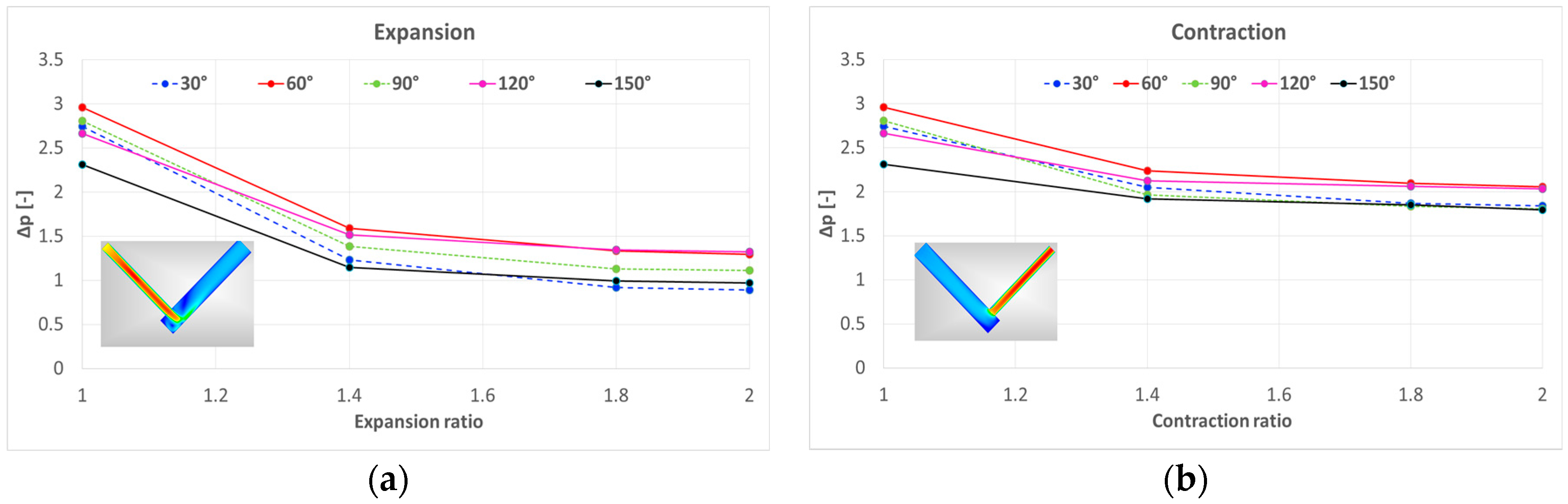
Figure 22.
Fluid velocity intensity map for different angle of the connection; expansion ratio of 2, reference fluid velocity 6.4 m/s (inlet flow rate 30 L/min).
Figure 22.
Fluid velocity intensity map for different angle of the connection; expansion ratio of 2, reference fluid velocity 6.4 m/s (inlet flow rate 30 L/min).
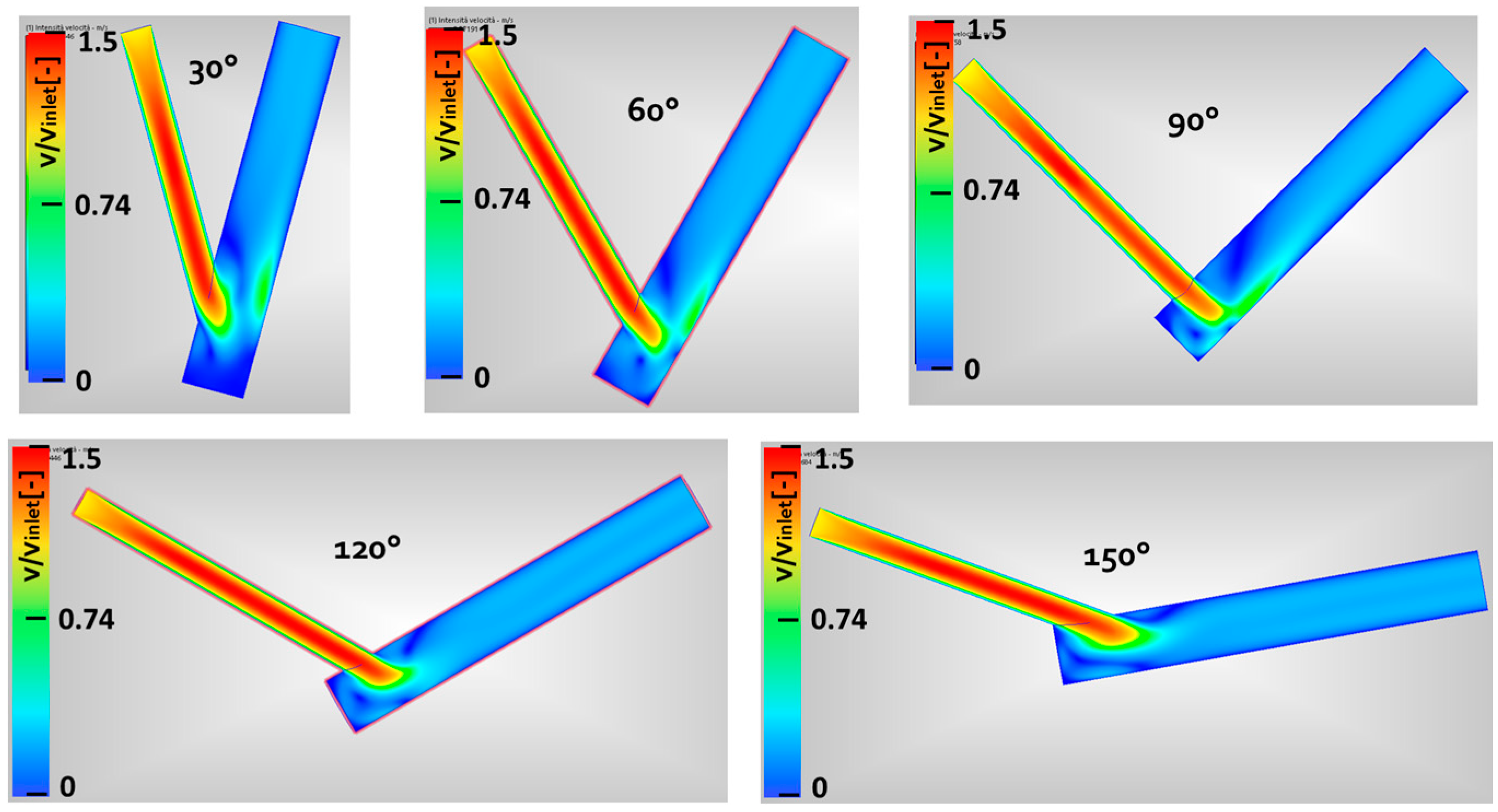
Figure 23.
Fluid velocity intensity map for different angle of the connection; contraction ratio of 2, reference fluid velocity 6.4 m/s (inlet flow rate 30 L/min).
Figure 23.
Fluid velocity intensity map for different angle of the connection; contraction ratio of 2, reference fluid velocity 6.4 m/s (inlet flow rate 30 L/min).


Table 1.
Mesh characteristics for the CFD analysis with a “mesh ratio” of 0.06.
| Mesh Ratio: Element Size/Minimum Channel Diameter | 0.06 |
| N° of elements U shape | 4,128,481 |
| N° of nodes U shape | 1,116,721 |
| N° of elements reversed S shape | 2,520,772 |
| N° of nodes reversed S shape | 713,811 |
| N° of elements twisted S shape | 2,470,316 |
| N° of nodes twisted S shape | 713,815 |
Table 2.
Sensors main characteristics.
| Sensor/Data Acquisition | Range | Accuracy |
|---|---|---|
| Piezoresistive pressure sensor | 0 ÷ 6 MPa, relative | 0.5% FS (0.03 MPa) |
| Piezoresistive pressure sensor | −0.1 ÷ 0.6 MPa, relative | 0.5% FS (0.0035 MPa) |
| Turbine flow meter | 7.5–75 L/min | 2.5% FS (1.69 L/min) |
| MULTI SYSTEM 5060 PLUS | 8 channels | - |
Table 3.
Fluid properties.
| Kinematic viscosity ν | 46 | cSt |
| Dynamic viscosity μ | 39.56 | cP |
| Temperature T | 40 | °C |
| Density ρ | 860 | kg/m3 |
Table 4.
Geometrical characteristics of the two paths.
| 5 Elbows Path | L (mm) | L/d | 6 Elbows Path | (mm) | L/d |
|---|---|---|---|---|---|
| Length 1–2 | 10.7 | 1.8 | Length 1–2 | 9 | 1.5 |
| Length 2–3 | 15.8 | 2.6 | Length 2–3 | 22.2 | 3.7 |
| Length 3–4 | 36.5 | 6.1 | Length 3–4 | 38.8 | 6.5 |
| Length 4–5 | 42.8 | 7.1 | Length 4–5 | 13 | 2.2 |
| Length 5–6 | 35.3 | 5.9 | Length 5–6 | 44.3 | 7.4 |
| Length 6–7 | 25 | 4.2 | Length 6–7 | 13.7 | 2.3 |
| Length 7–8 | 9 | 1.5 |
Table 5.
Mesh characteristics for the CFD analysis with a “mesh ratio” of 0.06.
| Mesh Ratio: Element Size/Minimum Channel Diameter | 0.06 |
| N° of elements 5 elbows path | 3,303,339 |
| N° of nodes 5 elbows path | 843,670 |
| N° of elements 6 elbows path | 3,768,511 |
| N° of nodes 6 elbows path | 973,570 |
Table 6.
Parameters used in the DOE analysis.
| Factors | ||||
|---|---|---|---|---|
| Center-to-Center Distance | Angle | Velocity (m/s) | Kinematic Viscosity (cSt) | |
| Levels | 3D | 30° | 0.64 (3 (L/min)) | 22 |
| 5D | 45° | 2.55 (12 (L/min)) | 46 | |
| 10D | 60° | 5.09 (24 (L/min)) | 100 | |
| 75° | 10.19 (48 (L/min)) | |||
| 90° | ||||
| 105° | ||||
| 120° | ||||
| 135° | ||||
| 150° | ||||
Table 7.
Example of the mesh characteristics for the CFD analysis for the V bends, for a “mesh ratio” of 0.06.
Table 7.
Example of the mesh characteristics for the CFD analysis for the V bends, for a “mesh ratio” of 0.06.
| Mesh Ratio:Element Size/Minimum Channel Diameter | 0.06 |
| N° of elements | 1460 K |
| N° of nodes | 384 K |
Table 8.
Parameters used in the analysis of the V-bend with expansion and contraction.
| Reference Diameter d | Fluid Velocity | Re | Viscosity |
|---|---|---|---|
| 10 mm | 6.4 m/s | 1391 | 46 cSt |
© 2017 by the authors. Licensee MDPI, Basel, Switzerland. This article is an open access article distributed under the terms and conditions of the Creative Commons Attribution (CC BY) license (http://creativecommons.org/licenses/by/4.0/).
Share and Cite
MDPI and ACS Style
Zardin, B.; Cillo, G.; Borghi, M.; D’Adamo, A.; Fontanesi, S. Pressure Losses in Multiple-Elbow Paths and in V-Bends of Hydraulic Manifolds. Energies 2017, 10, 788. https://doi.org/10.3390/en10060788
AMA Style
Zardin B, Cillo G, Borghi M, D’Adamo A, Fontanesi S. Pressure Losses in Multiple-Elbow Paths and in V-Bends of Hydraulic Manifolds. Energies. 2017; 10(6):788. https://doi.org/10.3390/en10060788
Chicago/Turabian StyleZardin, Barbara, Giovanni Cillo, Massimo Borghi, Alessandro D’Adamo, and Stefano Fontanesi. 2017. "Pressure Losses in Multiple-Elbow Paths and in V-Bends of Hydraulic Manifolds" Energies 10, no. 6: 788. https://doi.org/10.3390/en10060788
Note that from the first issue of 2016, this journal uses article numbers instead of page numbers. See further details here.