
Design and Implementation of Low-Power Analog-to-Information Conversion for Environmental Information Perception


1
School of Computer Science & Technology, Nanjing University of Posts and Telecommunications, Nanjing 210003, China
2
Jiangsu High Technology Research Key Laboratory for Wireless Sensor Networks, Nanjing 210003, China
*
Author to whom correspondence should be addressed.
Energies 2017, 10(6), 753; https://doi.org/10.3390/en10060753
Submission received: 22 March 2017
/
Revised: 17 May 2017
/
Accepted: 22 May 2017
/
Published: 27 May 2017
Abstract
:Because sensing nodes typically have limited power resources, it is extremely important for signals to be acquired with high efficiency and low power consumption, especially in large-scale wireless sensor networks (WSNs) applications. An emerging signal acquisition and compression method called compressed sensing (CS) is a notable alternative to traditional signal processing methods and is a feasible solution for WSNs. In our previous work, we studied several data recovery algorithms and network models that use CS for compressive sampling and signal recovery. The results were validated on large data sets from actual environmental monitoring WSNs. In this paper, we focus on the hardware solution for signal acquisition and processing on separate end nodes. We propose the paradigm of an analog-to-information converter (AIC) based on CS theory. The system model consists of a modulation module, filtering module, and sampling module, and was simulated and analyzed in a MATLAB/Simulink 7.0 environment. Further, the hardware design and implementation of an improved digital AIC system is presented. We also study the performances of three different greedy data recovery algorithms and analyze the system power consumption. The experimental results show that, for normal environmental signals, the new system overcomes the Nyquist limit and exhibits good recovery performance with a low sampling frequency, which is suitable for environmental monitoring based on WSNs.
1. Introduction
Due to the rapid economic development of China, environmental pollution affected by transportation and industry is becoming one of the biggest problems in China’s society today. With the help of those information and communication technologies (ICTs), how to monitor and control the environment pollution effectively has gained much attention from academia and industry, and is becoming a hot research issue. As one of such ICTs, wireless sensor networks (WSNs) [1] involves many procedures as data collection, information processing, network transmission and it is being widely used in almost every aspect of smart city such as environmental monitoring, smart homes, health monitoring, intelligent transportation and so on. However, there are still some bottlenecks about WSNs. When the scale of WSNs is keeping expanding, the costs of transmission and energy consumption increase significantly. In order to solve these problems, scholars are looking for ways, some of which are related with the theory of signal processing.
In the past several decades, Shannon sampling theorem is a core component of modern digital signal processing, having an important influence on both signal acquisition and processing. This theorem states that it is sufficient to sample the original signal at twice its bandwidth (known as the Nyquist rate) to ensure faithful recovery [2,3]. As a new emerging theory, compressed sensing (CS) offers us a striking alternative to traditional Shannon sampling theorem [4,5,6,7]. Various studies and applications on CS have been conducted in the research areas such as WSNs [8,9,10,11,12], image processing [13], radar [14], underwater communication [15], and health monitoring [16]. However, most of these work are focused on CS theory. The problem of designing high-efficiency hardware with limited energy is becoming a bottleneck in practical applications. Some scholars have attempted to solve this problem. For example, an analog-to-information converter (AIC), which is a non-correlation measurement scheme for CS, has been proposed in [17,18,19,20,21,22]. The details of these work will be discussed in Section 2.
In our previous work [23,24,25,26], we focused on software solution on network, which aims at designing suitable compressive algorithms or network models to solve the problem of data acquisition during transmission in large distributed WSNs. Another alternative way to decrease the energy consumption and transmission costs is designing low-power AIC device on separate end node for compressive signal acquisition by reducing the sampling rate of signal, which is our target in the work of this paper, and we name it hardware solution on end node. To the best of our knowledge, the present work introduces four main contributions.
- In view of the signal in real world, we design an AIC model and construct it in MATLAB/Simulink environment.
- Due to our main target applications are embedded systems based WSNs for environmental monitoring, we design and implement an improved digital AIC architecture on an embedded development platform according to the requirements of environmental monitoring application.
- Three different greedy algorithms are studied to optimize recovering the data collected by AIC and we make a comparison of the performance among them as well.
- We perform an exhaustive performance and power analysis between presented AIC architecture and traditional sampling method on the Nyquist rate in order to quantify the potential of applying CS in low-power sensing, compression and transmission.
The remainder of this paper is organized as follows. Some related work is introduced in Section 2. Section 3 introduces some background knowledge of CS, including CS model, architecture of AIC, and signal recovery method. Section 4 demonstrates a simulation model of AIC, which is built in MATLAB/Simulink environment. The hardware design of an improved digital AIC based on embedded system is described in Section 5. Section 6 presents three greedy algorithms in data recovery and makes a comparison of their performance. From the experiment result, we confirm the sparsity adaptive matching tracing pursuit (SAMP) is relatively optimal in our application. The power analysis is discussed in detail in Section 7 and the conclusions of the paper are presented in Section 8.
2. Related Work
Because various methods can be used to reduce power consumption on a WSN node, there are many studies on WSN power consumption and optimization for prolonging the lifetime of a network. For example, research on protocols to minimize energy consumption during network activities has gained increasing attention [27]. These power management schemes often focus on the duty cycling, where certain segments are set to a sleep state during idle mode [28]. Average power consumption is shown to be significantly reduced in [29] using an analytical criterion to optimize the synchronization duty. In [30], to determine the optimal conditions for transmitter power control, a comprehensive analysis on WSN modules is presented that considers power consumption, RF propagation measurement, and RSM analysis and optimization. A notable alternative approach to energy-saving in WSNs is based on the massive multiple-input multiple-output (MIMO) framework. For example, reference [31] analyzed the energy reduction laws for channel-aware decision fusion and employed massive MIMO framework for decentralized detection. In addition, some sub-optimal fusion rules were studied for a virtual MIMO channel in [32], which seemed to be more suitable for practical implementation and WSN energy budget reduction. Considering the path loss and uncertainty caused by estimated channel-state information, and the large antenna-array at a decision fusion center, reference [33] proposed some low-complexity sub-optimal rules to alleviate the severe energy constraints imposed on sensor nodes. To optimize the estimation problem in decentralized multi-sensor system, reference [34] proposed an optimal power allocation to reduce the total power consumption, and [35,36] analyzed the energy detection test used for MIMO decision fusion.
In [4], Candes proposed CS theory for the first time. CS theory states that, if the original signal is sparse, it can be reconstructed accurately at sampling rates well below the Nyquist rate by solving an optimization problem. Donoho offered a mathematical solution to the problem [5], which established the foundation of CS theory. In the last decade, there have been many interesting studies on a broad range of CS applications. For example, reference [14] applied CS to a radar system to acquire and reconstruct the high-dimensional image data. Moreover, the study proposed a novel architecture for a CS radar detector system that enables radar to be controlled adaptively under unknown noise and clutter. In another example, the authors in [21] investigated the potential of the CS signal acquisition/compression paradigm for ECG compression. The applications of CS in WSNs has attracted much attention as well. For example, reference [8] suggested using CS to take advantage of the possible joint sparsity of multiple sensor signals. In [10], the adoption of CS was suggested to address the data gathering problem in WSNs by considering the routing and network topology. Both [11,12] utilize the LEACH algorithm in WSNs, reference [11] performed node clustering and data recovery using Bayesian CS, and [12] used CS to improve the process of random sampling.
The theory of distributed compressed sensing (DCS), which considers the potential correlation of measurements at different nodes to extend a WSNs’ area, has drawn increasing research attention. The authors of [37] proposed a DCS theoretical framework that combines the theory of distributed source coding and CS to extend the use of CS in multi-signal distributed WSNs. In addition, the authors presented three joint sparsity models to characterize the fundamental performance limits of DCS recovery. Practical algorithms for the joint recovery of multiple signals in each proposed model were also given. Of these models, JSM-2 is studied widely in those applications in which multiple sensors obtain the same signal but with different phases and attenuation because of signal propagation, such as in MIMO communication and acoustic localization [38]. Moreover, reference [39] presented a new distributed algorithm based on sparse random projections that dose not need global coordination. In addition, reference [40] presented a DCS and data-fusion based data aggregation model and algorithm to improve the sensing precision and reduce the number of transmissions.
Studies on this topic have also been performed by our group. In [23,24], water quality and air quality monitoring systems based on distributed WSNs were presented. These systems support the acquisition and online monitoring via a PC or smart phone of conventional water and air quality measures like temperature, humidity, PM2.5, pH value, depth, electrolyte levels, and turbidity. However, with limited power storage in an outdoor deployment, the lifecycle of the system is effectively determined by the battery energy consumption. Therefore, how to decrease the energy consumption to prolong the network lifetime is the focus of our work. In [25], we proposed a model for data acquisition by combining CS and hierarchical routing. Furthermore, a quantitative mathematical analysis of the proposed model and a corresponding framework were presented. The experimental results showed that our solution is effective in large distributed WSNs. In [26], we introduced a novel solution using CS and the online recovery of large data sets and presented a new framework called the data acquisition framework of compressive sampling and online recovery (DAF-CSOR). Moreover, we compared the performance of three different greedy algorithms within DAF-CSOR.
In summary, the related studies and work mentioned above mostly make progress in the utilization of CS in WSNs in the view of improving the network routings, models, and algorithms during data transmission. Hardware design and implementation of CS-based signal acquisition on separate end device is a striking alternative on the other hand. There are a number of interesting studies aimed at implementing the data acquisition systems at sub Nyquist rate, which is called analog-to-information converter (AIC for short in this paper) normally. The authors of [17,18,19,20] introduced a new scheme of AIC system, named random demodulator (RD), which was constructed by readily available and robust components. In [20], the authors offered a theoretical analysis in detail to support the empirical observations from the viewpoint of system preformance. Meanwhile, the authors in [17] presented a complete transistor-level realization for AIC based on RD. Moreover, references [18,19] proposed a RD-based AIC system which uses modulation, filtering, and sampling, which made it possible for hardware implementation. For the high frequency signal from applications such as ultra wide band (UWB), reference [22] proposed a novel AIC architecture, named random modulation pre-integrator (RMPI) with the state-of-the-art RD, while the experiments with a discussion of possible hardware implementation was presented too in that paper. Considering further reducing the complexity as well as power consumption of state-of-the-art AIC system, reference [21] presented a new scheme in the application of ECG compression, spread spectrum random modulator pre-integrator (SRMPI), which used spread spectrum prior to random modulation. Summarizing, the work in this paper is inspired thanks to the related studies about AIC.
3. Background of CS
3.1. CS Model
In CS theory, the original physical signal can be represented as a vector , where N is the vector length. Specifically, let X be expanded via a basis , such that
where and . is an invertible transformation matrix of size . If has K nonzero coefficients and , then X is said to be K-sparse and denotes a sparse dictionary.
The output signal of compressive measurement can be rewritten as the product of a matrix and a vector through random sampling, that is
where refers to linear observations obtained through random sampling and is measurement matrix when .
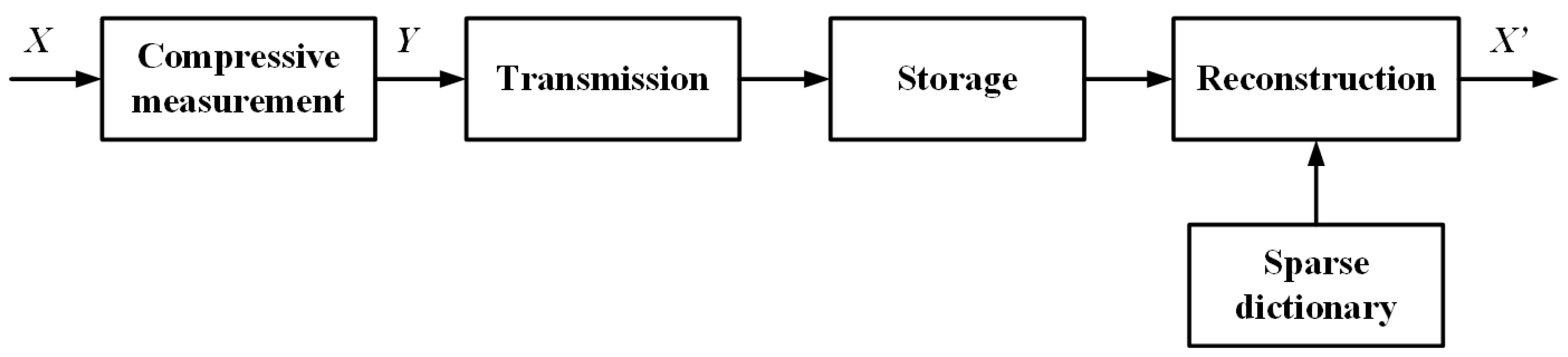
It is important to remark that the measurement matrix does not rely on the signal itself. In other words, a simple linear sampling adaptive strategy is provided, which is only marginally off for the optimal but complex for the best. The procedure of CS sampling is shown in Figure 1.
To ensure the smooth reconstruction of the original signals, two conditions must be satisfied [5,6].
Condition 1.
The input signal must be expressed in a certain domain, following
where is the coherence coefficient between the measurement matrix Φ and the sparse dictionary Ψ, which measures the maximum correlation between any two elements of the two matrices. To recover the signal accurately, experience suggests that at least four unrelated samples are needed for each nonzero term, so that .
Condition 2.
The measurement matrix Φ should obey the key restricted isometry property (RIP) [4]
For any K-sparse vector α, exists, is the recovery matrix.
In general, Bernoulli matrix, sub-Gaussian random measurement matrix, and Gaussian white noise matrix are the measurement matrices used most commonly, which have same characteristics that the matrix elements follow a certain distribution independently. A small number of observations is required during accurate reconstruction as a result of the fact that those measurement matrices are irrelevant to the most sparse signals.
3.2. AIC Architecture
With the rapid development of information science, traditional analog-to-digital converter (ADC) designed according to Shannon sampling theorem face severe challenges. First, some applications of radio frequency (RF) systems need to sample high-frequency signals, which requires the use of high speed ADC. This is difficult with the current ADC design technology. Second, even for low signal bandwidths, sampling at the Nyquist rate might collect large amounts of redundant information, resulting in a waste of the limited resources and power of the system.
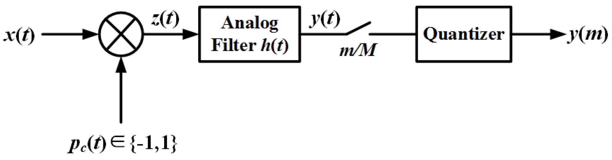
As introduced before, the CS-based signal acquisition system at sub-Nyquist rate, which is called analog-to-information converter (AIC) is studied in many related work in order to solve above problems. The benefit of this method is that the analog signals are sampled directly using a wide band pseudo random modulator and a low-speed sampler without analog-to-digital conversion. By considering the compromise of every aspect in our application such as circuit complexity, cost, characteristics of the original signal, we choose RD-based AIC to study in this work. The basic RD architecture [17,18,19,20] of AIC is shown in Figure 2. The procedure can be divided into three steps including signal modulation, filtering, and sampling.
Modulation This stage uses a modulator whose input signal is multiplied by a continuous time sequence of pseudo random numbers to obtain an output signal .
Filtering In this stage, a low-pass filter is used as a simple accumulator to sum the modulated signal over a period of seconds. According to Shannon sampling theorem, the ideal symbol conversion rate of is greater than or equal to the Nyquist rate of the original input signal .
Sampling The final stage utilizes a standard ADC and a quantizer to sample the filter output signal every seconds to obtain the digital signal .
It can be further simplified as
3.3. Signal Recovery
With the sampled vector Y by AIC and the measurement matrix , it is possible to estimate the sparse coefficient by solving a problem through a reconstruction algorithm which can be written as
where is the recovery matrix and written as
In general, the minimization described in Equation (9) is an NP-hard issue that can not be effectively resolved. There are two types of reconstruction algorithms commonly used today: -based convex optimization algorithms and -based greedy algorithms. One typical example of a greedy algorithm is matching pursuit (MP) [41], while the main convex optimization algorithms are the base tracking algorithm and gradient projection reconstruction algorithm. Although a convex optimization algorithm provides a better reconstruction, it requires larger transmission consumption, higher algorithm complexity and lower reconstruction speed than greedy algorithm. Considering the characteristics of WSNs and the limited resources in our application, we prefer to use a -based greedy algorithm for data reconstruction. Researchers have made a lot of effort to optimize the performance of classic MP, resulting in many improved algorithms, such as orthogonal matching pursuit (OMP) [42], regularized orthogonal matching pursuit (ROMP) [43,44], sparsity adaptive matching tracing pursuit (SAMP) [45], and compression sampling matching pursuit (CoSaMP) [46].
4. System Simulation
4.1. System Modeling
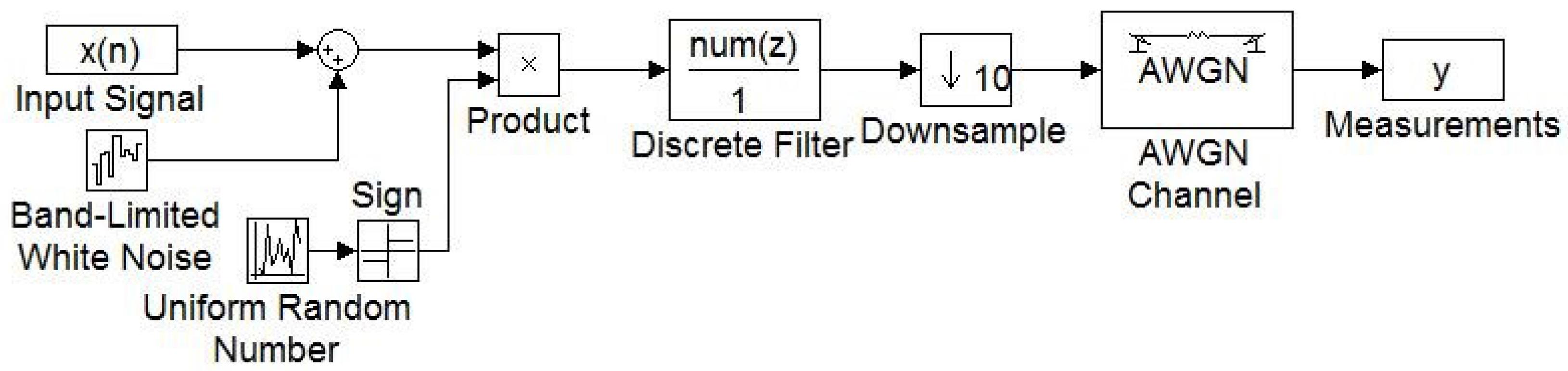
The construction of an AIC simulation model based on RD architecture in Figure 2 in MATLAB/Simulink soft environment is described in this section. The AIC system model mainly consists of a signal source, noise source, pseudo random sequence generator, multiplier, low-pass filter, and ADC, as shown in Figure 3.
The original signals, which are collected by sensors in the natural environment, are stored in a text file and read by the signal source. The noise includes two parts, one is from the signal source and another from the transmission channel. The noise is filtered out from the original signals in amplification, so that the additive noise of the source is band-limited white noise.
4.2. Simulation Analysis
In order to quantify the compression performance in the assessment of following simulation results, three commonly used performance parameters, the compression ratio (), the related recovery error (), and signal-to-noise ratio () are introduced. is defined as
where and are the required bits’ number for the original and compressed signals. The , and associated , represent error between the original signal vector X and the recovered signal vector X’, can be written as
In our proposed system, the recovery algorithm is realized by programming. The main performance indexes of the model are obtained from a simulation test of the multi-group data. The AIC simulation process is illustrated in Figure 4.
First, the original sparse signal of length is generated, as shown in Figure 4a. Assuming the input is 18 dB, the sparsity (i.e., the original signal contains 10 important signal components), and the maximum frequency is 500 Hz, the symbol conversion rate of the pseudo random sequence of should be 1000 Hz at least, as shown in Figure 4b. In this simulation, we use the observation number , which means . The output signals are obtained after signal modulation, filtering, and sampling, which are illustrated in Figure 4c–e, respectively. Figure 4f shows the reconstructed signal x’, which is obtained using SAMP. The output of the reconstructed signal x’ reached 17 dB. The results show that the proposed AIC model can successfully compress the sparse signal and recover the original signal well. This method supports the reliable signal construction when the input is as low as 7 dB.
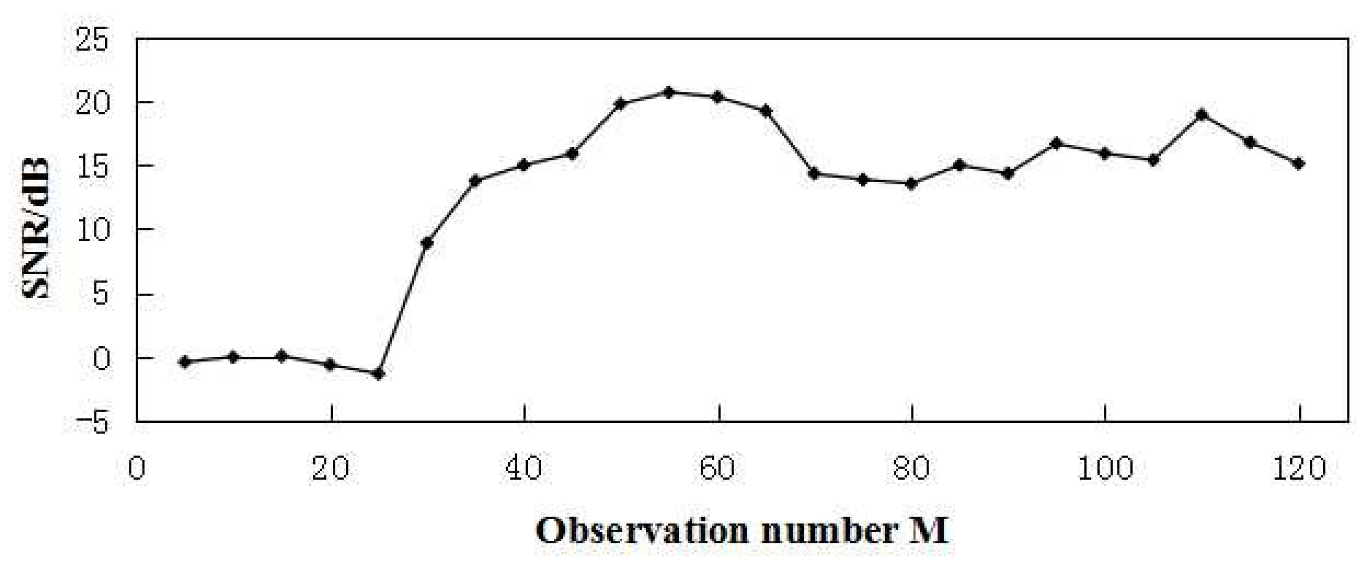
For further analysis, the system performance is tested under K = 4 and 8 with different observation numbers. The simulation and reconstruction results are presented in Table 1 and Figure 5, where M stands for the observation number.
From the results above, it can be seen that when , the output is less than 10 dB when (i.e., is greater than 96.5%). However, when , the output is less than zero, which means the original signal cannot be recovered precisely. When (i.e., is less than 96.5%), the output is greater than 13.78 dB, and reaches a maximum of 20.74 dB. The system performance is tested in the same way when . When (i.e., is greater than 98%), the output is less than 1 dB, and the original signal fails to recover accurately.
By analyzing the simulation results, we have verified that, in practical applications, the relationship between M and K described in Equation (3) can be approximated as . When , values of 4, 8, and 10 require M to be greater than 16, 32, and 40, respectively. Table 1 and Figure 5 show that when , sparse signals can be compressed and reconstructed. In addition, when the sparsity is lower, is higher. To obtain a higher , the observation number M should be as small as possible. However, considering the accuracy of the reconstruction, the observation number M should be greater than in practical situation.
4.3. Experiment Results
To evaluate the validity and reliability of the proposed AIC system, we have carried out some experiments to sample the water temperature data from a 5-day period as the original data. The average daily water temperature exhibits an upward trend with a certain cyclical component and the initial output signals of the temperature sensor range from 60 to 100 mV. Through three stages of amplification, the original signal , the amplitude of which is 330–450 mV, is shown in Figure 6a. It is able to obtain its corresponding signal in frequency domain through Discrete-Time Fourier Transform (DFT), as shown in Figure 7, where stands for sampling frequency. In practice, Fast Fourier Transform (FFT) is used in programming instead of DFT to reduce the complexity of algorithm. Seen from Figure 7, we could get that the sparsity K is 18 approximately by ignoring those signals in very small value. Since the fact that such important signal components within the domain of low frequency, sufficient information could be obtained because the symbol conversion rate of the pseudo random sequence is greater than the Nyquist sampling rate of the original signal. In this experiment, , and the observation number . Thus, is 90%. Figure 6b–f show the various stages of CS using AIC, including the pseudo random sequence signal, modulated output signal, filter output signal, sampled output signal, and reconstructed signal. The experimental result in Figure 6f shows that the reconstructed signal is able to recover the original signal accurately. The input is 18 dB, and the output is 16.91 dB.
5. Hardware Design of AIC System
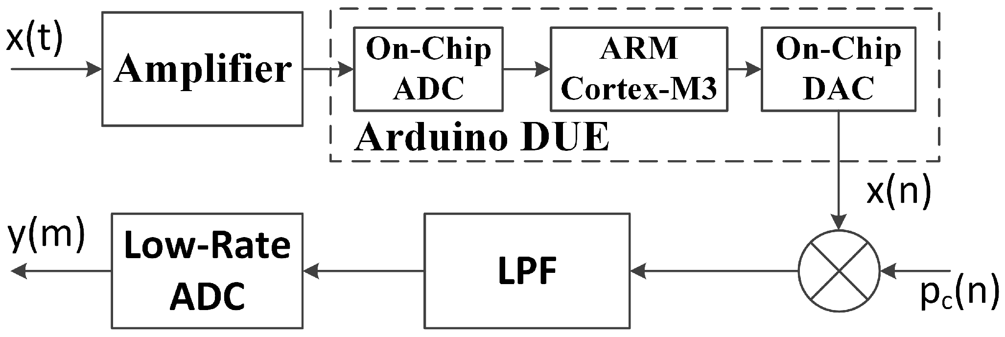
Our proposed AIC system is designed to process environmental parameters such as temperature, humidity, and pH value signals, which have the characteristics of low frequency and high sparsity. In such practical applications, the AIC system will not put too much pressure on the ADC in terms of data sampling. However, with the emergence of an increasing number of digital sensors, it is more convenient to use discrete signals in signal processing. In view of this situation, the traditional RD-based AIC model in Figure 2 is modified and we propose an improved digital AIC system shown in Figure 8.
In that improved digital AIC system, the original signal is amplified and preprocessed before modulation. The output signal of most environmental sensors is very weak, e.g., the E201-C pH sensor (INESA Scientific Instrument, Shanghai, China), which has a low-frequency output signal of just a few millivolts. It is impossible to collect such weak signals without amplifying, filtering, and other processing. Thus, an integrated operational CA3140 amplifier (Intersil, San Jose, CA, USA) is chosen to amplify the signal, and we use Arduino DUE development platform (Arduino, Turin, Italy) for preprocessing, which has a good balance between low power consumption and rich resources. The preprocessed signal is sampled by the internal low-rate 12-bit ADC of an on-board Cortex-M3 ARM processor (Atmel, San Jose, CA, USA). Then, the on-chip 12-bit DAC converts the processed data to the discrete original signal .
The built-in Linear Feedback Shift Register (LFSR) of the ARM processor is used to generate a pseudo random sequence. In its code, the function randomSeed() is utilized to initialize the random number generator with a fairly random input, such as analogRead() on an unconnected analog pin. If analog input pin 0 is unconnected, random analog noise will cause the call to randomSeed() to generate different seed numbers each time. Every time a pseudo random number 0 or 1 is generated, a low or high voltage value, respectively, is written into the digital output port pin. The frequency of the pseudo random sequence is controlled by the delay time. A flow chart of the pseudo random sequence generation is illustrated in Figure 9.
The digital output port of ARM processor can generate a sequence of random numbers of . In order to obtain a Bernoulli matrix, a subtraction circuit is designed using an operational amplifier to get the required signal, which is shown in Figure 10.
could be calculated according to
In order to meet the requirement of impedance matching, appropriate resistances are selected in Figure 10 according to Equation (13). Figure 11 shows the signals measured by mixed domain oscilloscope MDO4034 (Tektronix, Johnston, SC, USA), in which Arduino generated original signal with blue color and the output pseudo random sequence from the conversion circuit with red color.
An AD633 multiplier (Analog Devices, Norwood, MA, USA) is used to modulate the discrete input signal and pseudo random sequence , which spreads the spectrum of the original signal. The amplitude of the pseudo random sequence is V with 1000 Hz symbol conversion rate, which can effectively sample sensor signal within 500 Hz.
Taking into account the actual situation, a low-pass filter replaces the integrator. A Chebyshev filter can effectively remove the high-frequency interference signal because its frequency response is better than that of other filters. A bipolar active filter is used to reduce the power consumption and loading effect of filtering. Because the signal decrease 10 times in the AD633 multiplier, the two-staged voltage-controlled low-pass filter is designed to overcome that attenuation, as shown in Figure 12.
The transfer function for this filter is
where constants B and C are normalized coefficients, g is the voltage gain and is the cut-off frequency.
Finally, an ADC circuit is designed using the 12-bit serial AD converter chip AD7898 (Analog Devices, Norwood, MA, USA) to sample the output signal of the filter. The ARM microprocessor (Atmel, San Jose, CA, USA) then reads the output signal after sampling and quantization, and thus determines the actual observation.
The proposed improved digital AIC system does effectively reduce the output rate of system data. Furthermore, the structure of the existing data measurement scheme is relatively unchanged. In this design, we use the internal LFSR of the ARM microprocessor to generate the pseudo random sequence, rather than using the components to construct an LFSR [17] or using an FPGA, which further reduces the cost and complexity of the system. It should be noted that the sampling period of the ADC circuit must be precisely adjusted, otherwise the characteristics of the measurement matrix cannot be fully identified. This may result in the system not reconstructing the original signal accurately. Compared with the sampling period of the ADC, the time deviation of the system must be small enough to effectively reduce the time error so that the system performs better at low frequency.
6. Data Reconstruction
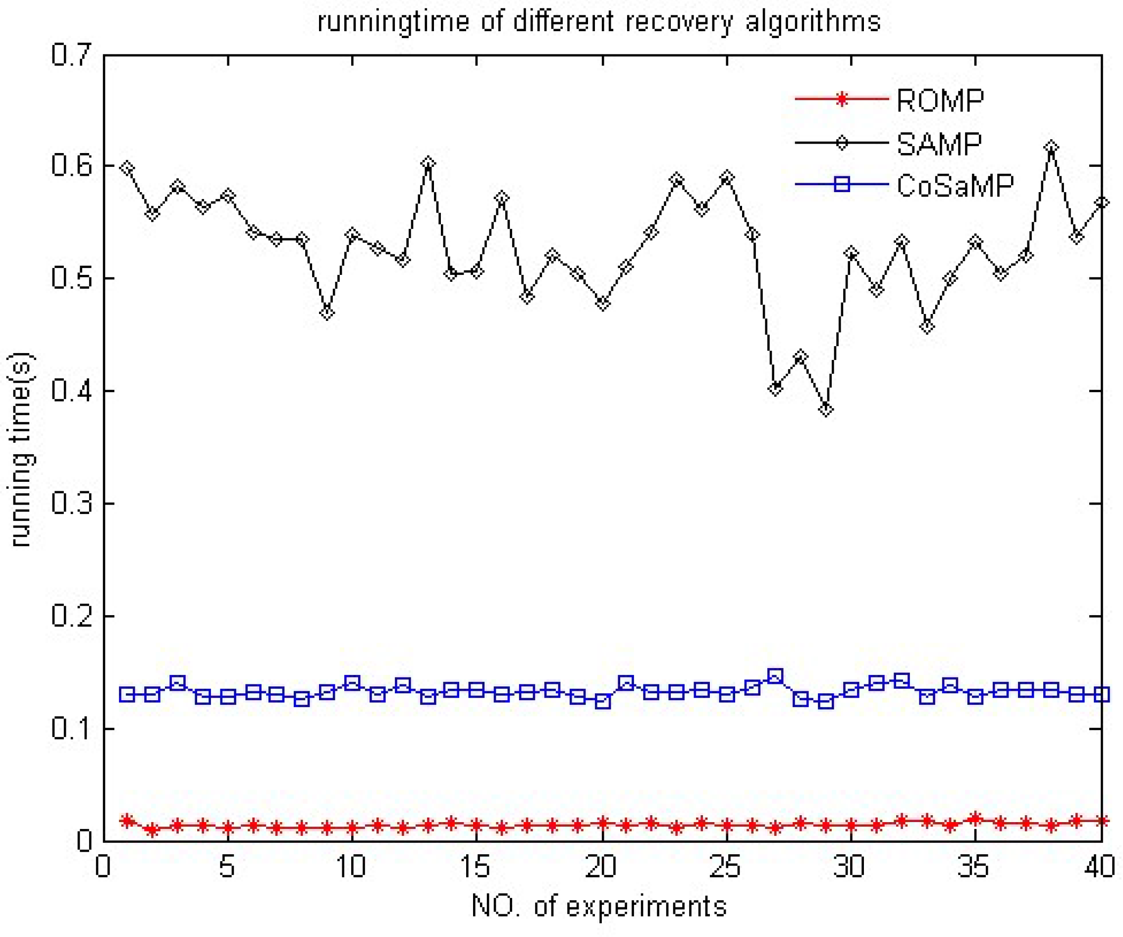
Data reconstruction plays a very important role in our project. In this section, we study three -based greedy algorithms, ROMP, SAMP, and CoSaMP. The reconstruction performance of these three algorithms is first compared in Figure 13. For this simulation, the original signal was collected in our designed monitoring WSN system [23,24]. We then used the RD-based AIC system simulation model presented in Section 4 to obtain the sampled output signal as the input of reconstruction. The simulation soft environment was MATLAB 7.0.
In Figure 13, the blue and red lines represent the original and recovered signals, respectively. Because of their different atomic selection strategies and iteration stop conditions, the performance of the three algorithms differs. The relative error and running time of the three algorithms are measured and compared in Figure 14 and Figure 15, respectively.
The relative recovery error () is calculated according to Equation (11). Figure 14 shows that the SAMP provides an obviously lower than the other two recovery algorithms thanks to its backtracking and improved atomic selection procedure. Thus, SAMP has the capability of sparsity-adaptive.
In Figure 15, the results show that ROMP has best running time performance and CoSaMP also performs well. The running time of SAMP is the worst because it is constrained by the step length. However, when the step length is modified so that its sparsity is close to that of the real data, the running time is improved significantly. In our application, because the data reconstruction work on the sink node without energy limit, there is no influence on the lifetime of the end node.
In summary, to balance reconstruction accuracy with running time, we conclude that SAMP is the best choice mainly because of its sparsity-adaptive capability, which adapts the reconstruction to the signals with unknown sparsity that often occur in practice.
7. Power Analysis
In this section, several power consumption models for evaluating our system design are introduced. We compare and analyze the power consumption of the ADC and AIC during signal sampling and wireless transmission, respectively, as illustrated in Figure 16.
7.1. Power Analysis in Signal Sampling
During the stage of signal sampling (SS), the theoretic power models of ADC and AIC are denoted as and , and calculated as follows [47].
where is the signal bandwidth, is ADCs figure-of-merit, and are constants, and is the amplifier gain. In addition, N, M, , and are the tunable parameters for the AIC system, while only and can be tuned in the ADC. Note that should be set differently for the ADC and AIC systems. In the ADC system, the input signal is sampled directly by the ADC at the Nyquist sampling rate. On the other hand, it is an accumulated signal from the integrator that is sampled by the ADC device in the AIC system. Because the accumulated signal is larger than the original, the required could be significantly lower in the AIC system than in the ADC system. Another difference concerns parameter , which is used to measure the power per sample per effective number of quantization steps. Because of the fact that the ADC in the AIC system normally works at a much lower frequency, it has a smaller than the ADC system does [47].
For our application, because of the features of the original input signal such as low frequency, medium resolution, and small amplitude, we adopt the AIC system for the main purpose of data compression. Here our desirable target is for compression. The main simulation parameters of the AIC system are shown in Table 2.
Figure 17 compares the power consumption of the ADC and AIC during signal sampling. The results show that although the power consumption of the mixers and integrator in the AIC is significant compared with the ADC, the AIC system is successfully able to reduce the overall sampling cost. The AIC system reduces the overall power consumption by compared with a traditional ADC at the Nyquist sampling rate.
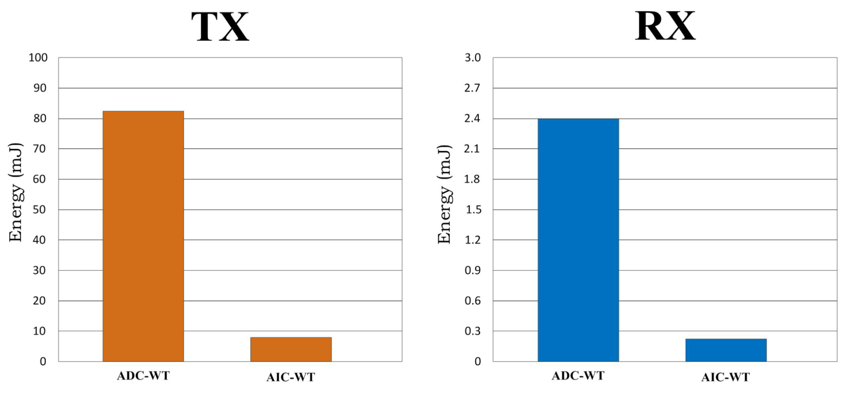
7.2. Power Analysis in Wireless Transmission
The wireless transmission (WT) model [48], which includes data transmission (TX) and data reception (RX) is shown in Figure 18.
The simplified energy models of the ADC and AIC for TX and RX are denoted by , , and , , respectively, and defined as follows [49,50].
In wireless communication, the power consumption depends on the communication distance and data bits, which are denoted as d and b. The TX energy consumption involves two parts, the energy cost of circuit , and the cost of amplifier . Only is included in the RX energy consumption. The XBee S2C produced by DIGI company was selected as the wireless communication module. It uses the ZigBee protocol. Some parameters from its datasheet are listed Table 3.
Because of its strong signal compression ability, a node using the AIC system sends and receives much less data during TX and RX, resulting in significantly reduced energy-consumption. Assuming the data size is 1024 bits in transmission and the communication distance is 100 m, Figure 19 shows the energy consumption of the system using the AIC and ADC in the TX and RX stages.
8. Conclusions
This paper presented a CS-based signal acquisition system that solves the limited energy problem of sensor nodes in environmental monitoring WSNs. With state-of-the-art work related to CS and AIC, we constructed an RD-based AIC architecture and corresponding simulation model in the MATLAB/Simulink environment. In addition, the improved digital AIC system was designed and implemented using an embedded system for the first time. Three different recovery algorithms were also studied to evaluate the reconstruction of the signal from our proposed AIC system. Finally, power consumption of the AIC and traditional ADC during signal sampling and wireless transmission was compared. The experiment results show that our proposed AIC system overcomes the Nyquist limit and exhibits good recovery performance when using a low-complexity greedy algorithm, which is suitable for environmental monitoring WSNs.
Acknowledgments
We thank the financial support provided by the National Nature Science Foundation of P.R.China (Grant Nos. 61401221, 61572261, 61572260, 61373017, 51608437, 51541804), China Postdoctoral Science Foundation (Grant No. SBH16024), Scientific & Technological support project of Jiangsu Province (Grant Nos. BE2014718, BE2015702). Especial thanks due to Jiao Hu for assistance with the experiments and to Phillip James Haberman for assistance in English-language editing.
Author Contributions
All authors have participated in preparing the research from the beginning to the end. Study design, modelling, simulaton, analyses, writing: Shu Shen, Yue Shan, and Jian Sun; analyses, writing: Lijuan Sun, Zhiqiang Zou, and Ruchuan Wang.
Conflicts of Interest
The authors declare no conflict of interest.
References
- Pottie, G.J.; Kaiser, W.J. Wireless integrated network sensors. Commun. ACM 2000, 43, 51–58. [Google Scholar] [CrossRef]
- Landau, H.J. Sampling, data transmission, and the Nyquist rate. Proc. IEEE 1967, 55, 1701–1706. [Google Scholar] [CrossRef]
- Landau, H.J. Necessary density conditions for sampling and interpolation of certain entire functions. Acta Math. 1967, 117, 37–52. [Google Scholar] [CrossRef]
- Candes, E.J.; Romberg, J.; Tao, T. Robust uncertainty principles: Exact signal reconstruction from highly incomplete frequency information. IEEE Trans. Inf. Theory 2006, 52, 489–509. [Google Scholar] [CrossRef]
- Donoho, D. Compressed sensing. IEEE Trans. Inf. Theory 2006, 52, 1289–1306. [Google Scholar] [CrossRef]
- Candes, E.J.; Wakin, M. An introduction to compressive sampling. IEEE Signal Process. Mag. 2008, 25, 21–30. [Google Scholar] [CrossRef]
- Tsaig, Y.; Donoho, D. Extensions of compressed sensing. Signal Process. 2006, 86, 549–571. [Google Scholar] [CrossRef]
- Yang, A.Y.; Gastpar, M.; Bajcsy, R.; Sastry, S.S. Distributed sensor perception via sparse representation. Proc. IEEE 2010, 98, 1077–1088. [Google Scholar] [CrossRef]
- Bajwa, W.; Haupt, J.; Sayeed, A.M.; Nowak, R.D. Joint source-channel communication for distributed estimation in sensor networks. IEEE Trans. Inf. Theory 2007, 53, 3629–3653. [Google Scholar] [CrossRef]
- Quer, G.; Masiero, R.; Munaretto, D.; Rossi, M.; Widmer, J.; Zorzi, M. On the interplay between routing and signal representation for compressive sensing in wireless sensor networks. In Proceedings of the 2009 Information Theory and Applications Workshop, San Diego, CA, USA, 8–13 February 2009; pp. 206–215. [Google Scholar]
- Tang, L.; Zhou, Z.; Shi, L.; Yao, H.P.; Zhang, J. Source detection in wireless sensor network by LEACH and compressive sensing. J. Beijing Univ. Posts Telecommun. 2011, 34, 8–11. [Google Scholar]
- Zhang, J.C.; Lv, F.X.; Wang, Y.; Wang, Q.; Tang, Y.K. Compressive sensing based on clustering network in WSNs. Chin. J. Sci. Instrum. 2014, 35, 169–177. [Google Scholar]
- Bourquard, A.; Unser, M. Binary compressed imaging. IEEE Trans. Image Process. 2013, 22, 1042–1055. [Google Scholar] [CrossRef] [PubMed]
- Anitori, L.; Maleki, A.; Otten, M.; Baraniuk, R.G.; Hoogeboom, P. Design and analysis of compressed sensing radar detectors. Signal Process. 2013, 61, 813–827. [Google Scholar] [CrossRef]
- Fazel, M.; Fatemeh, F.; Stojanovic, M. Random access compressed sensing for energy-efficient underwater sensor networks. IEEE J. Sel. Areas Commun. 2011, 29, 1660–1670. [Google Scholar] [CrossRef]
- Mamaghanian, H.; Khaled, N.; Atienza, D.; Vandergheynst, P. Compressed sensing for real-time energy efficient ECG compression on wireless body sensor nodes. IEEE Trans. Biomed. Eng. 2011, 58, 2456–2466. [Google Scholar] [CrossRef] [PubMed]
- Laska, J; Kirolos, S; Duarte, M; Ragheb, T.S.; Baraniuk, R.G.; Massoud, Y. Theory and implementation of an analog-to-information converter using random demodulation. In Proceedings of the IEEE International Symposium on Circuits and Systems, New Orleans, LA, USA, 27–30 May 2007; pp. 1959–1962. [Google Scholar]
- Kirolos, S.; Ragheb, T.; Laska, J.; Duarte, M.; Massoud, Y.; Baraniuk, R.G. Practical issues in implementing analog-to-information converters. In Proceedings of the 6th International Workshop on System-on-Chip for Real-Time Applications, Cairo, Egypt, 27–29 December 2006; pp. 141–146. [Google Scholar]
- Kirolos, S.; Laska, J.; Duarte, M.; Baron, D.; Ragheb, T.; Massoud, Y.; Baraniuk, R.G. Analog-to-information conversion via random demodulation. In Proceedings of the IEEE Dallas/CAS Workshop on Design Applications, Integration and Software, Richardson, TX, USA, 29–30 October 2006; Volume 10, pp. 71–74. [Google Scholar]
- Tropp, J.; Laska, J.; Duarte, M.; Romberg, J.; Baraniuk, R. Beyond Nyquist: Efficient sampling of sparse bandlimited signals. IEEE Trans. Inf. Theory 2010, 56, 520–544. [Google Scholar] [CrossRef]
- Mamaghanian, H.; Khaled, N.; Atienza, D.; Vandergheynst, P. Design and Exploration of low-power analog to information conversion based on compressed sensing. IEEE J. Emerg. Sel. Top. Circuits Syst. 2012, 2, 493–501. [Google Scholar] [CrossRef]
- Naini, F.; Gribonval, R.; Jacques, L.; Vandergheynst, P. Compressive sampling of pulse trains: Spread the spectrum! In Proceedings of the IEEE International Conference on Acoustics, Speech and Signal Processing, Taipei, Taiwan, 19–24 April 2009; pp. 2877–2880. [Google Scholar]
- Shen, S.; Hu, J.; Zou, Z.Q.; Sun, J.; Lu, S.Y.; Wang, X.W. A distributed wireless sensor network for online water quality monitoring. Commun. Comput. Inf. Sci. 2015, 501, 685–697. [Google Scholar]
- Hu, J.; Sun, J.; Wang, X.W.; Shen, S.; Zou, Z.Q. Research on water environment monitoring system based on WSNs. Microcomput. Appl. 2015, 34, 60–63. [Google Scholar]
- Zou, Z.Q.; Hu, C.C.; Zhang, F.; Zhao, H.; Shen, S. WSNs data acquisition by combining hierarchical routing method and compressive sensing. Sensors 2014, 14, 16766–16784. [Google Scholar] [CrossRef] [PubMed]
- Zou, Z.Q.; Li, Z.T.; Shen, S.; Wang, R.C. Energy-efficient data recovery via Greedy algorithm for wireless sensor network. Int. J. Distrib. Sens. Netw. 2016, 501, 725639. [Google Scholar] [CrossRef]
- Anastasi, G.; Conti, M.; Francesco, M.D.; Passarella, A. Energy conservation in wireless sensor networks: A survey. Ad Hoc Netw. 2009, 7, 537–568. [Google Scholar] [CrossRef]
- Wang, J.; Chen, M.; Leung, V.C.M. Forming priority based and energy balanced ZigBee networks—A pricing approach. Telecommun. Syst. 2013, 52, 1281–1292. [Google Scholar] [CrossRef]
- Macii, D.; Agee, A.; Somov, A. Power consumption reduction in wireless sensor networks through optimal synchronization. In Proceedings of the IEEE Instrumentation and Measurement Technology Conference, Singapore, 5–7 May 2009; pp. 1346–1351. [Google Scholar]
- Horvat, G.; Sostaric, D.; Zagar, D. Response surface methdology based power consumption and RF propagation analysis and optimization on XBEE WSN module. Telecommun. Syst. 2015, 59, 437–452. [Google Scholar] [CrossRef]
- Ciuonzo, D.; Romamo, G.; Salvo Rossi, P. Performance analysis and design of maximum ratio combining in channel-aware MIMO decision fusion. IEEE Trans. Wirel. Commun. 2013, 12, 4716–4728. [Google Scholar] [CrossRef]
- Ciuonzo, D.; Romano, G.; Salvo Rossi, P. Channel-aware decision fusion in distributed MIMO wireless sensor networks: Decode-and-Fuse vs. Decode-then-Fuse. IEEE Trans. Wirel. Commun. 2012, 11, 2976–2985. [Google Scholar] [CrossRef]
- Ciuonzo, D.; Salvo Rossi, P.; Dey, S. Massive MIMO channel-aware decision fusion. IEEE Trans. Signal Process. 2015, 63, 604–619. [Google Scholar] [CrossRef]
- Shirazinia, A.; Dey, S.; Ciuonzo, D.; Salvo Rossi, P. Massive MIMO for decentralized estimation of a correlated source. IEEE Trans. Signal Process. 2015, 64, 2499–2512. [Google Scholar] [CrossRef]
- Ciuonzo, D.; Romano, G.; Salvo Rossi, P. Optimality of received energy in decision fusion over rayleigh fading diversity MAC with non-identical sensors. IEEE Trans. Signal Process. 2013, 61, 22–27. [Google Scholar] [CrossRef]
- Salvo Rossi, P.; Ciuonzo, D.; Kansanen, K.; Ekman, T. On energy detection for MIMO decision fusion in wireless sensor networks over NLOS fading. IEEE Commun. Lett. 2015, 19, 303–306. [Google Scholar] [CrossRef]
- Baron, D.; Duarte, M.F.; Wakin, M.B.; Sarvotham, S.; Baraniuk, R.G. Distributed Compressive Sensing. Available online: https://arxiv.org/abs/0901.3403 (accessed on 25 April 2017).
- Duarte, M.F.; Sarvotham, S.; Baron, D.; Wakin, M.B.; Baraniuk, R.G. Distributed compressive sensing of jointly sparse signals. In Proceedings of the Conference Record of the Thirty-Ninth Asilomar Conference on Signals, Systems and Computers, Pacific Grove, CA, USA, 30 October–2 November 2005; Volume 22, pp. 1537–1541. [Google Scholar]
- Duarte, M.F.; Wakin, M.B.; Baron, D.; Baraniuk, R.G. Universal distributed sensing via random projections. In Proceedings of the 5th International Conference Information Processing in Sensor Networks, Nashville, TN, USA, 19–21 April 2006; pp. 177–185. [Google Scholar]
- Kang, J.; Tang, L.W.; Zou, X.Z.; Li, A.H. Distributed compressed sensing-based data fusion in sensor networks. In Proceedings of the 1st International Conference Pervasive Computing Signal Processing and Applications, Harbin, China, 17–19 September 2010; pp. 1083–1086. [Google Scholar]
- Mallat, S.G.; Zhang, Z.F. Matching pursuits with time-frequency dictionaries. IEEE Trans. Signal Process. 1993, 41, 3397–3415. [Google Scholar] [CrossRef]
- Patti, Y.C.; Rezaiifar, R.; Krishnaprasad, P.S. Orthogonal matching pursuit: Recursive function approximation with applications to wavelet decomposition. In Proceedings of the 1993 Conference Record of the Twenty-Seventh Asilomar Conference on Signals, Systems and Computers, Pacific Grove, CA, USA, 1–3 Novomber 1993; pp. 40–44. [Google Scholar]
- Needell, D.; Vershynin, R. Uniform uncertainty principle and signal recovery via regularized orthogonal matching pursuit. Found. Comput. Math. 2009, 9, 317–334. [Google Scholar] [CrossRef]
- Needell, D.; Vershynin, R. Signal recovery from incomplete and inaccurate measurements via regularized orthogonal matching pursuit. IEEE J. Sel. Top. Signal Process. 2010, 4, 310–316. [Google Scholar] [CrossRef]
- Do, T.T.; Gan, L.; Nguyen, N.; Tran, T.D. Sparsity adaptive matching pursuit algorithm for practical compressed sensing. In Proceedings of the 42nd Asilomar Conference on Signals, Systems and Computers, Pacific Grove, CA, USA, 26–29 October 2008; pp. 581–587. [Google Scholar]
- Needell, D.; Tropp, J.A. CoSaMP: Iterative signal recovery from incomplete and inaccurate samples. Appl. Comput. Harmonic Anal. 2009, 26, 301–321. [Google Scholar] [CrossRef]
- Chen, F.; Chandrakasan, A.P.; Stojanovic, V.M. Design and analysis of a hardware-efficient compressed sensing architecture for data compression in wireless sensors. IEEE J. Solid State Circuits 2012, 47, 744–756. [Google Scholar] [CrossRef]
- Heinzelman, W.; Chandrakasan, A.; Balakrishnan, H. Energy-efficient communication protocol for wireless microsensor networks. In Proceedings of the 33rd Annual Hawaii International Conference on System Sciences, Maui, HI, USA, 7 January 2000; p. 223. [Google Scholar]
- Liu, D.H.; Cheng, H.Y. Analysis of lifetime of wireless sensor networks based on energy budget. J. Shandong Norm. Univ. 2015, 30, 38–42. [Google Scholar]
- Duartemelo, E.J.; Liu, M. Analysis of energy consumption and lifetime of heterogeneous wireless sensor networks. In Proceedings of the IEEE Global Telecommunications Conference, Taipei, Taiwan, 17–21 November 2002; pp. 21–25. [Google Scholar]
Figure 1.
The basic framework of CS sampling.

Figure 2.
The basic random demodulator (RD) architecture of analog-to-information converter (AIC).

Figure 3.
The RD-based AIC system model in MATLAB/Simulink.

Figure 4.
AIC system simulation process.
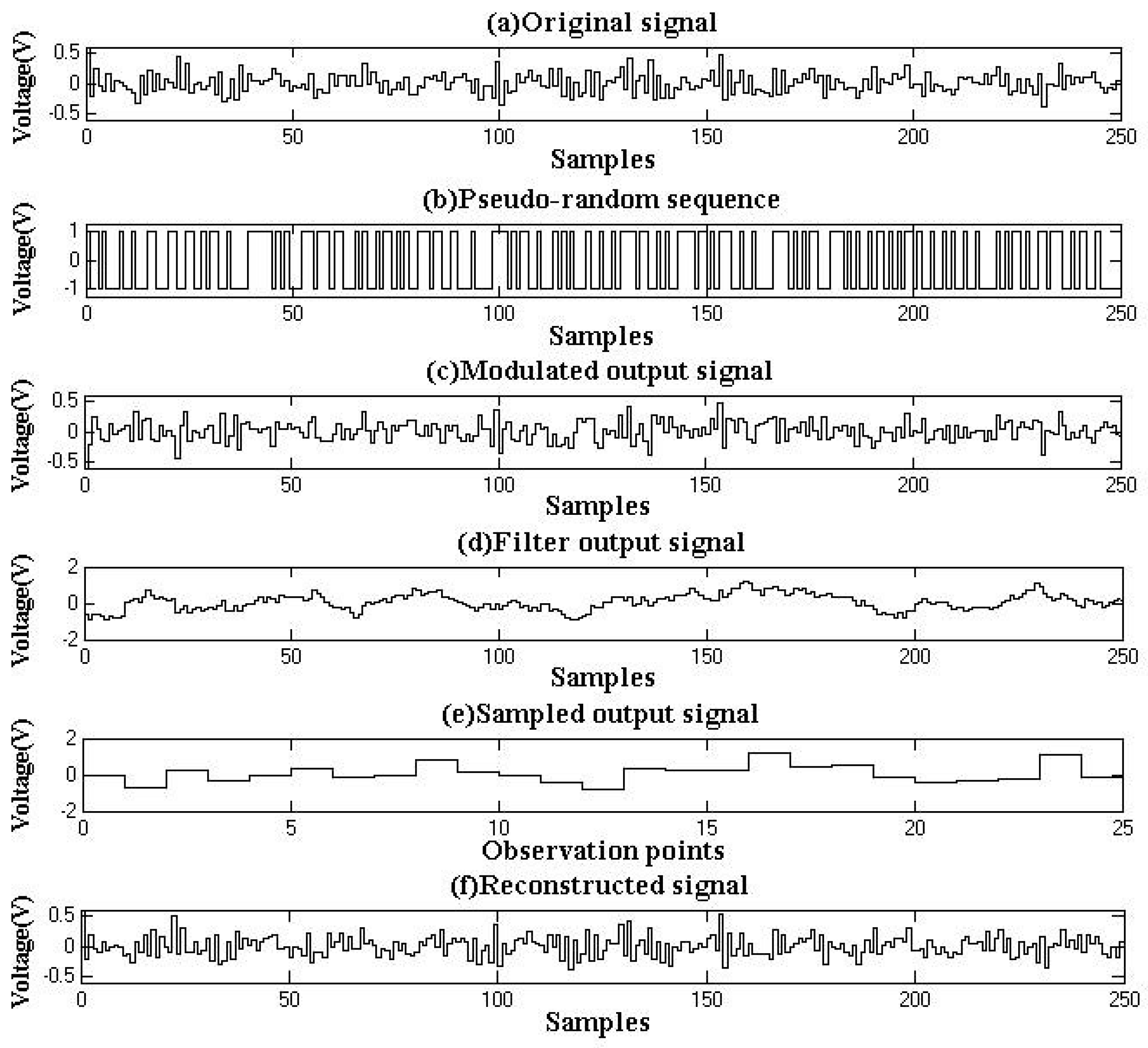
Figure 5.
AIC performance with different when .

Figure 6.
Experiment results.
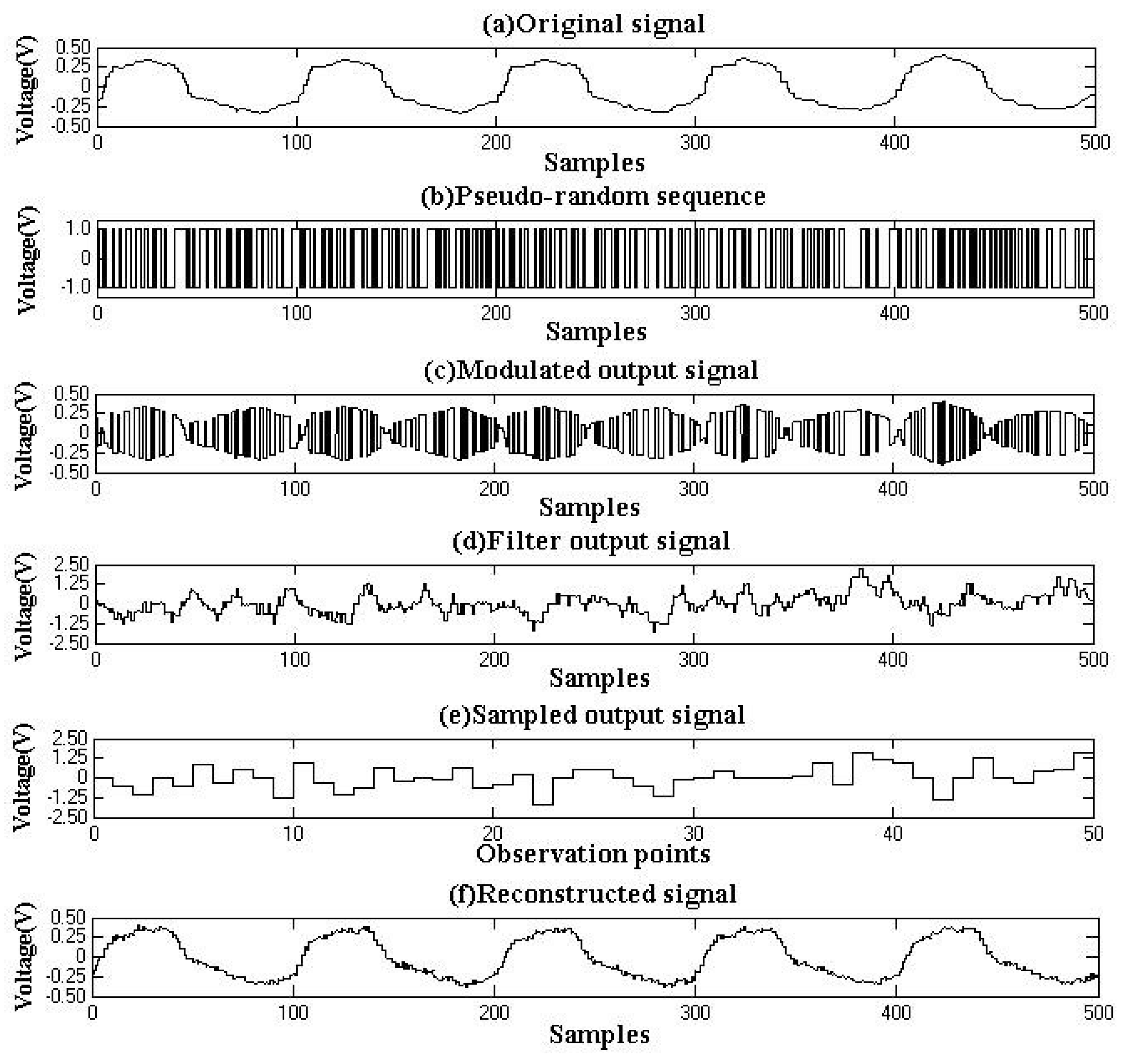
Figure 7.
Fourier spectrum .
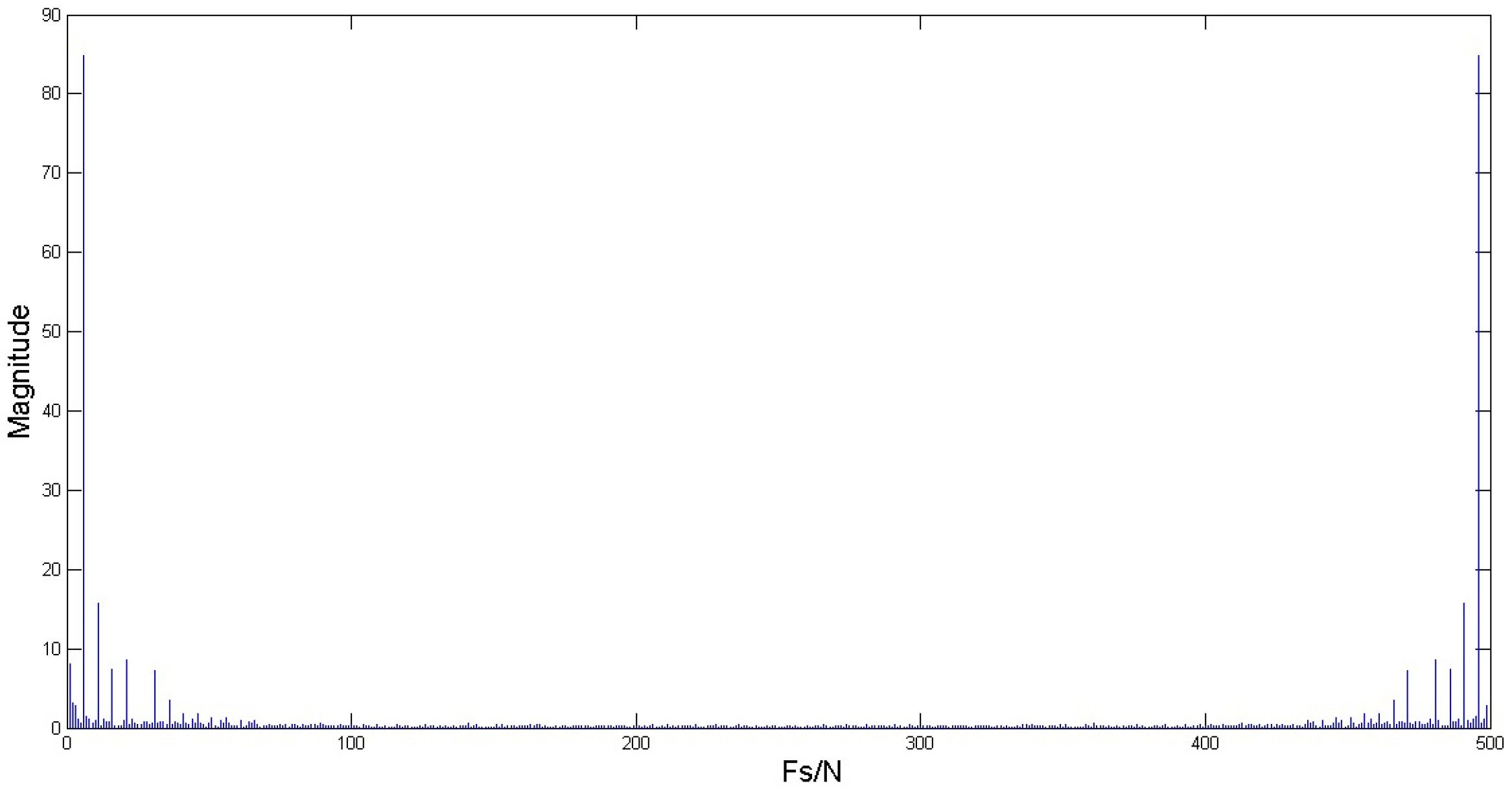
Figure 8.
Improved digital AIC system.

Figure 9.
Flow chart of pseudo random sequence’s generation.
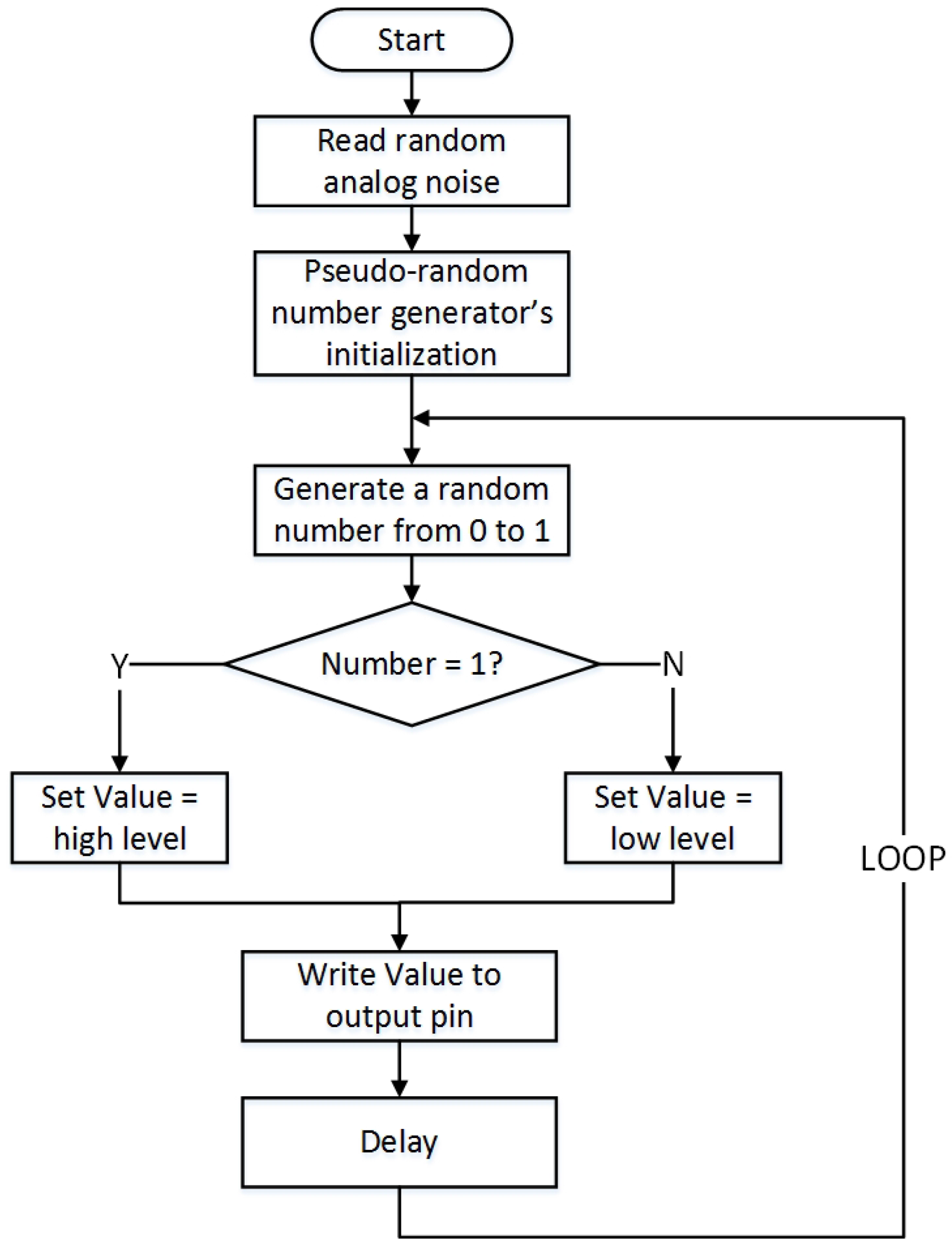
Figure 10.
Subtraction circuit for conversion from {0,1} to {−1,+1}.
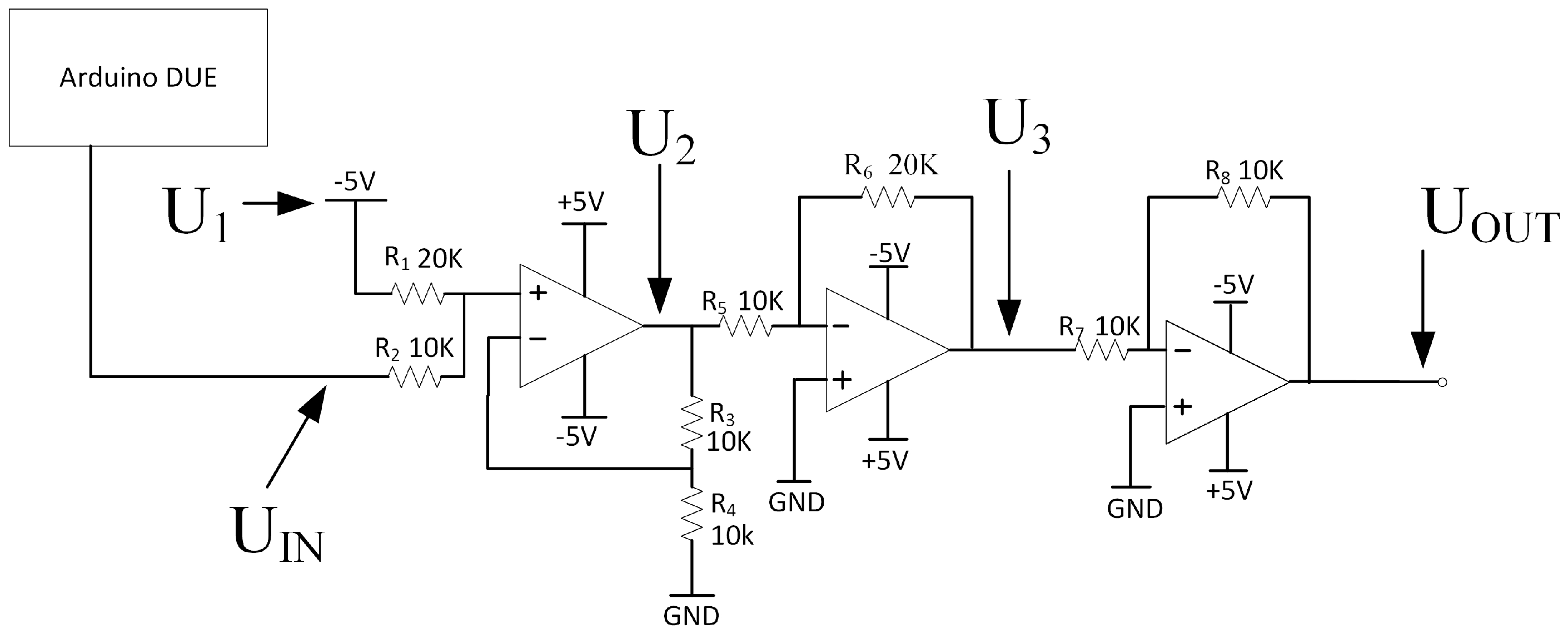
Figure 11.
Pseudo random sequence signals measured by MDO4034.
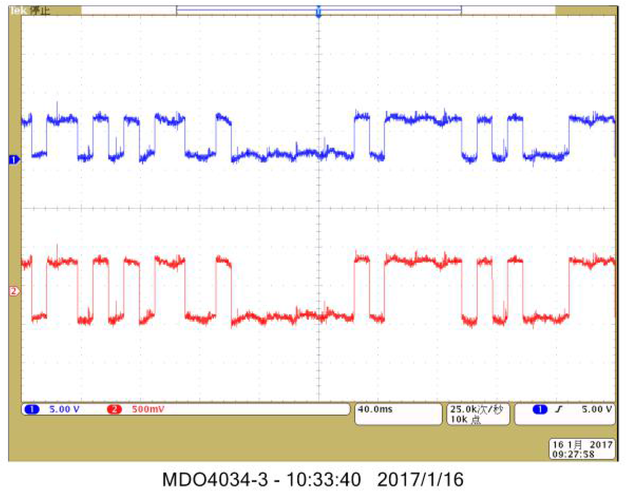
Figure 12.
Two staged voltage-controlled low-pass filter.
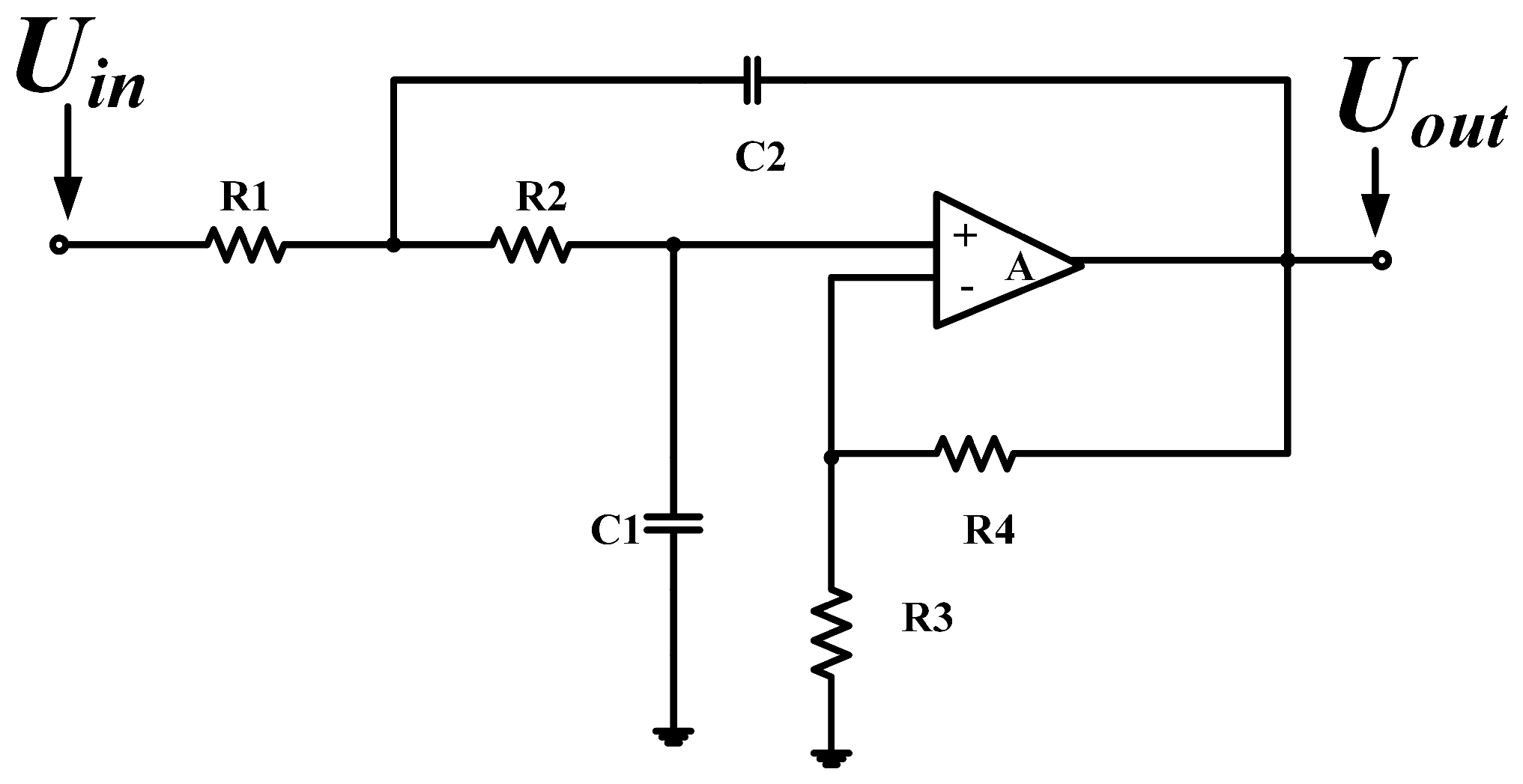
Figure 13.
Reconstruction performance of three recovery algorithms.
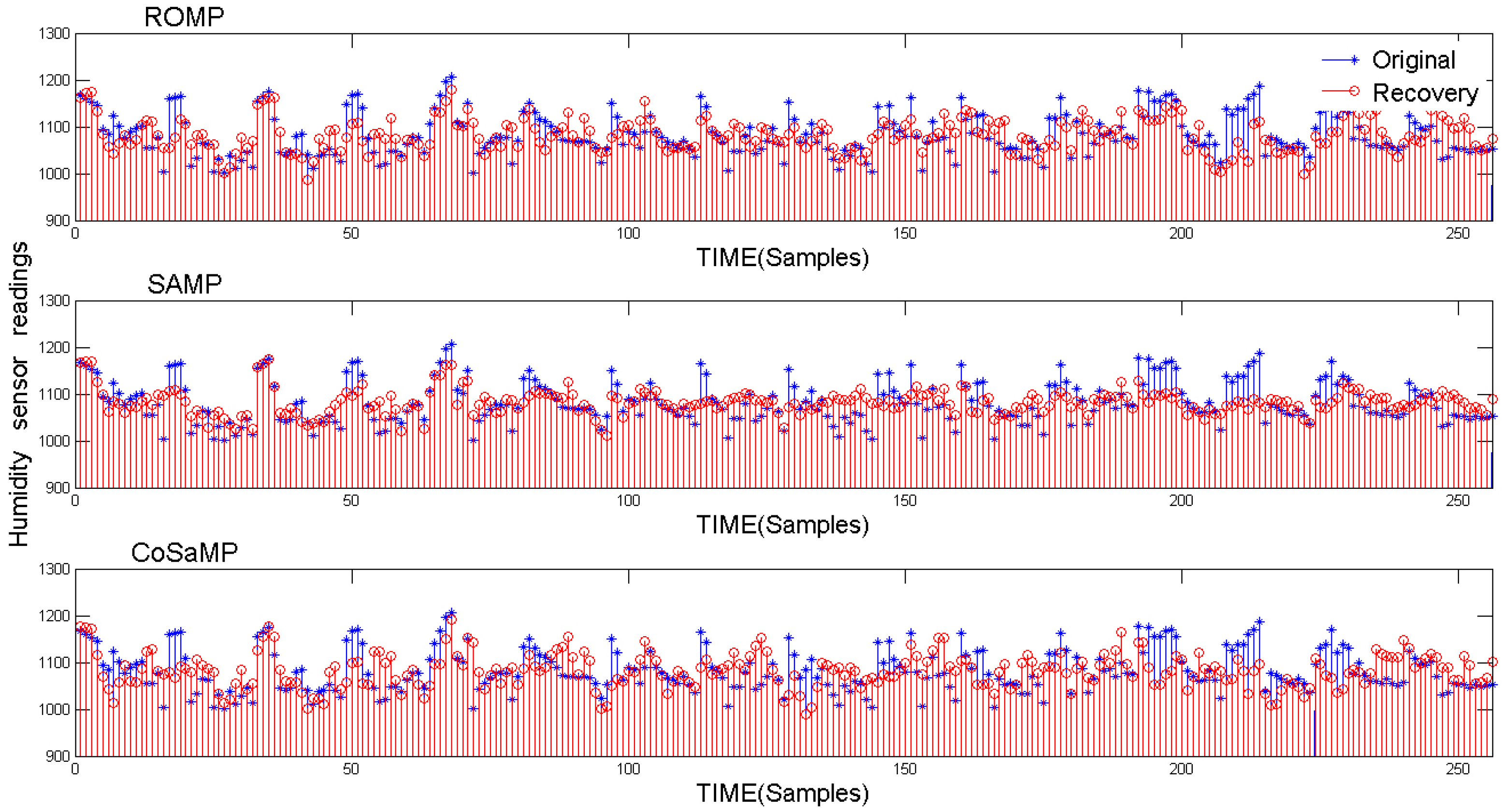
Figure 14.
Comparison of relative recovery error () among three recovery algorithms.
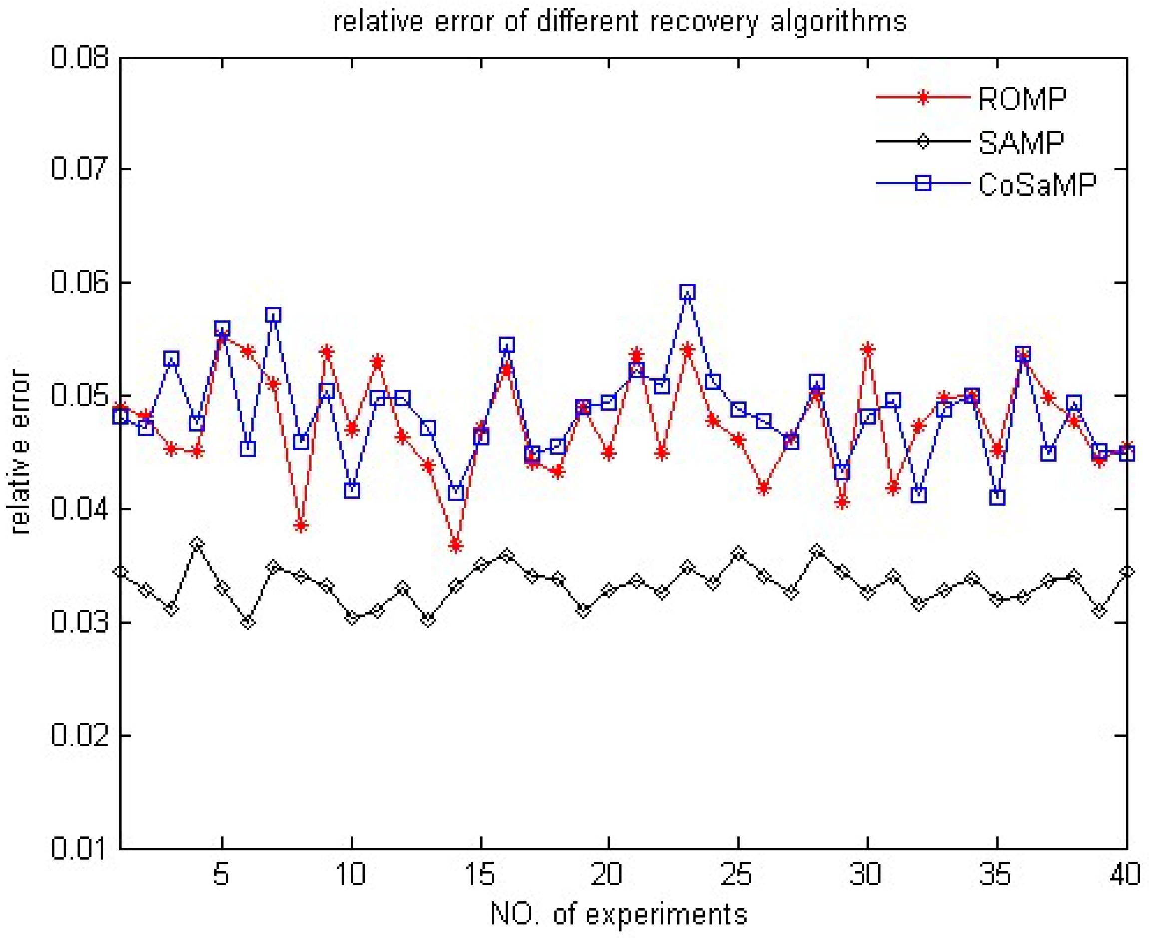
Figure 15.
Comparison of running time among three recovery algorithms.

Figure 16.
Architecture of the system.
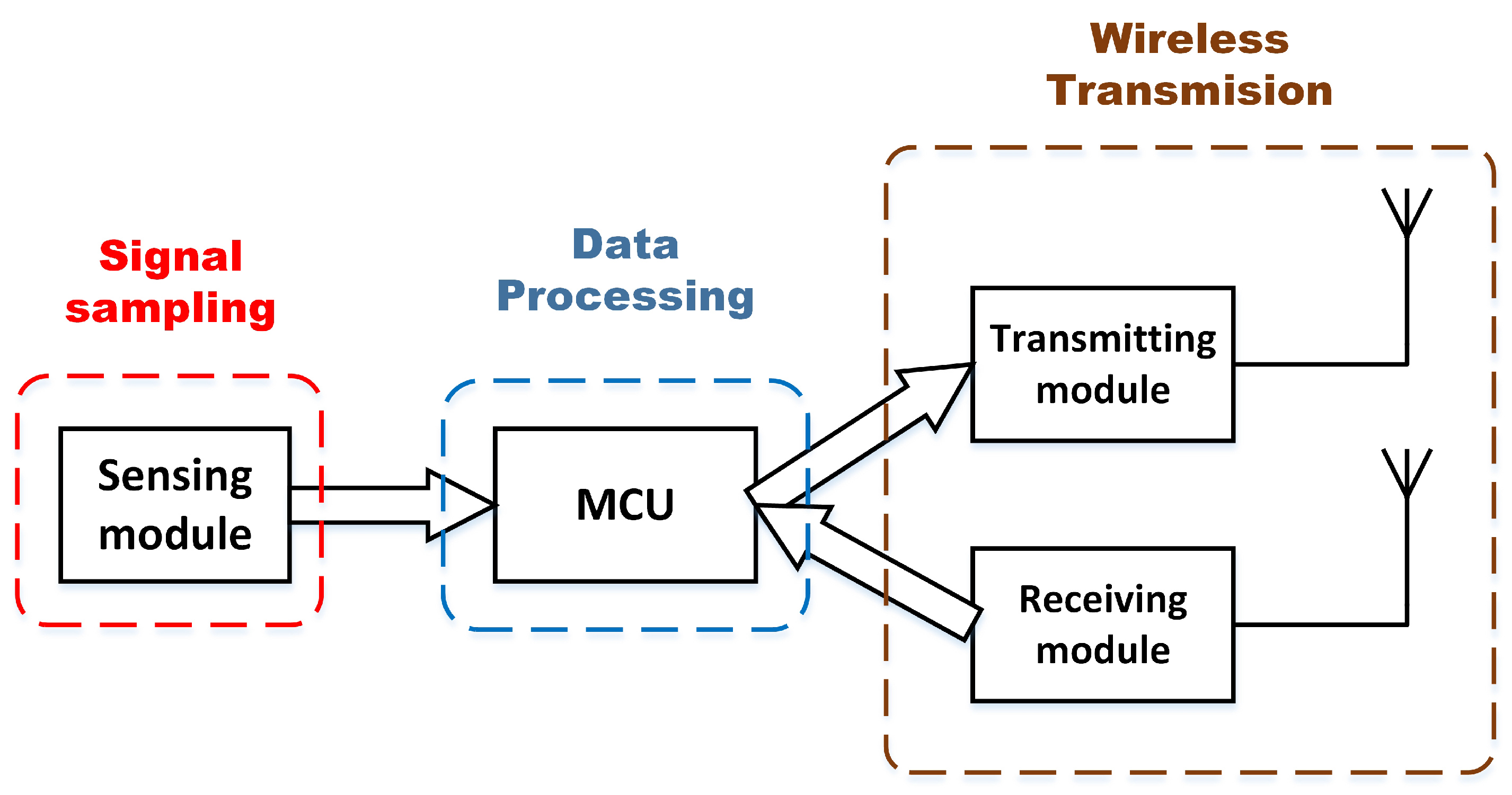
Figure 17.
Comparison of power consumption between analog-to-digital converter (ADC) and AIC system in signal sampling.
Figure 17.
Comparison of power consumption between analog-to-digital converter (ADC) and AIC system in signal sampling.
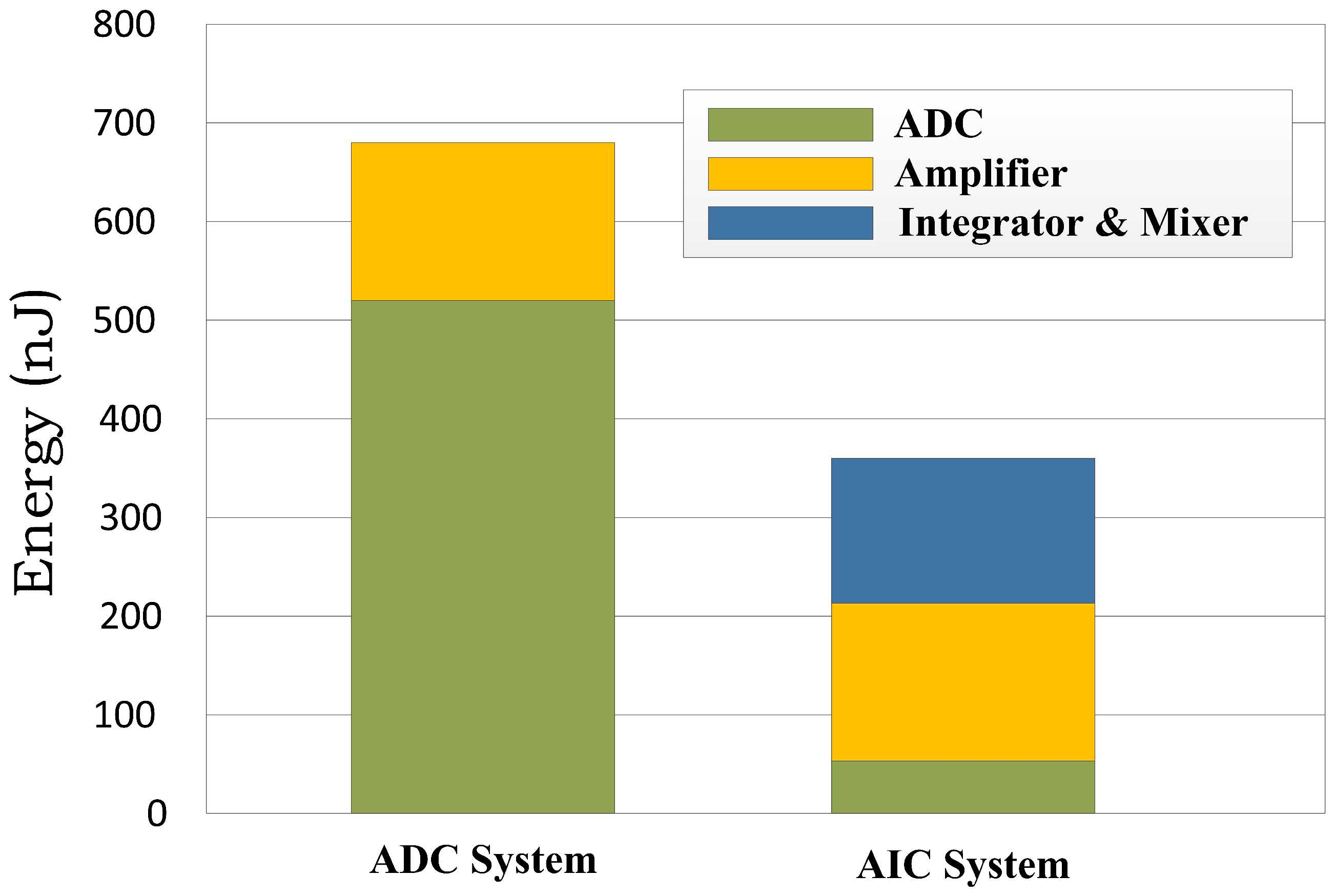
Figure 18.
Wireless transmission model.
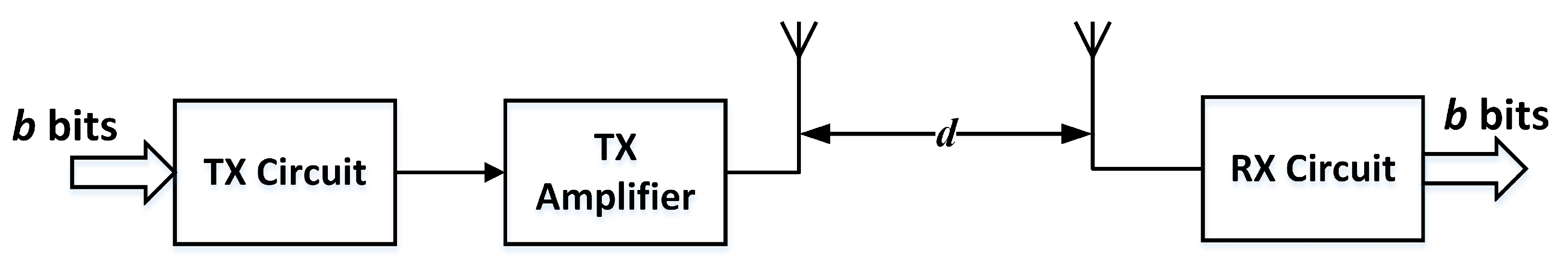
Figure 19.
Comparison of power consumption between ADC and AIC system in wireless transmission.


Table 1.
Simulation results under different with and .
| (%) | (dB) | (%) | (dB) | ||
|---|---|---|---|---|---|
| 20 | 98 | −0.67 | 5 | 99.5 | −0.61 |
| 25 | 97.5 | −1.37 | 10 | 99 | −0.18 |
| 30 | 97 | 8.91 | 15 | 98.5 | 0.01 |
| 35 | 96.5 | 13.78 | 20 | 98 | 16.88 |
| 40 | 96 | 15.01 | 25 | 97.5 | 14.65 |
| 45 | 95.5 | 15.91 | 30 | 97 | 18.78 |
| 50 | 95 | 19.83 | 35 | 96.5 | 15.92 |
| 55 | 94.5 | 20.74 | 40 | 96 | 19.73 |
| 60 | 94 | 20.37 | 45 | 95.5 | 18.64 |
| 65 | 93.5 | 19.28 | 50 | 95 | 18.05 |
Table 2.
AIC system simulation parameters for power consumption in sampling.
| Parameters | Value |
|---|---|
| M | 50 |
| N | 500 |
| 1 kHz | |
| 8 | |
| 5 | |
| 1 pJ/conversion-step |
Table 3.
Energy consumption of XBee S2C per bit when m.
| Parameters | Value |
|---|---|
| (μJ/bit) | 2.34 |
| (nJ/bit) | 7.8 |
© 2017 by the authors. Licensee MDPI, Basel, Switzerland. This article is an open access article distributed under the terms and conditions of the Creative Commons Attribution (CC BY) license (http://creativecommons.org/licenses/by/4.0/).
Share and Cite
MDPI and ACS Style
Shen, S.; Shan, Y.; Sun, L.; Sun, J.; Zou, Z.; Wang, R. Design and Implementation of Low-Power Analog-to-Information Conversion for Environmental Information Perception. Energies 2017, 10, 753. https://doi.org/10.3390/en10060753
AMA Style
Shen S, Shan Y, Sun L, Sun J, Zou Z, Wang R. Design and Implementation of Low-Power Analog-to-Information Conversion for Environmental Information Perception. Energies. 2017; 10(6):753. https://doi.org/10.3390/en10060753
Chicago/Turabian StyleShen, Shu, Yue Shan, Lijuan Sun, Jian Sun, Zhiqiang Zou, and Ruchuan Wang. 2017. "Design and Implementation of Low-Power Analog-to-Information Conversion for Environmental Information Perception" Energies 10, no. 6: 753. https://doi.org/10.3390/en10060753
Note that from the first issue of 2016, this journal uses article numbers instead of page numbers. See further details here.