
The Effect of Embodied Impact on the Cost-Optimal Levels of Nearly Zero Energy Buildings: A Case Study of a Residential Building in Thessaloniki, Greece


Abstract
:1. Introduction
2. Materials and Methods
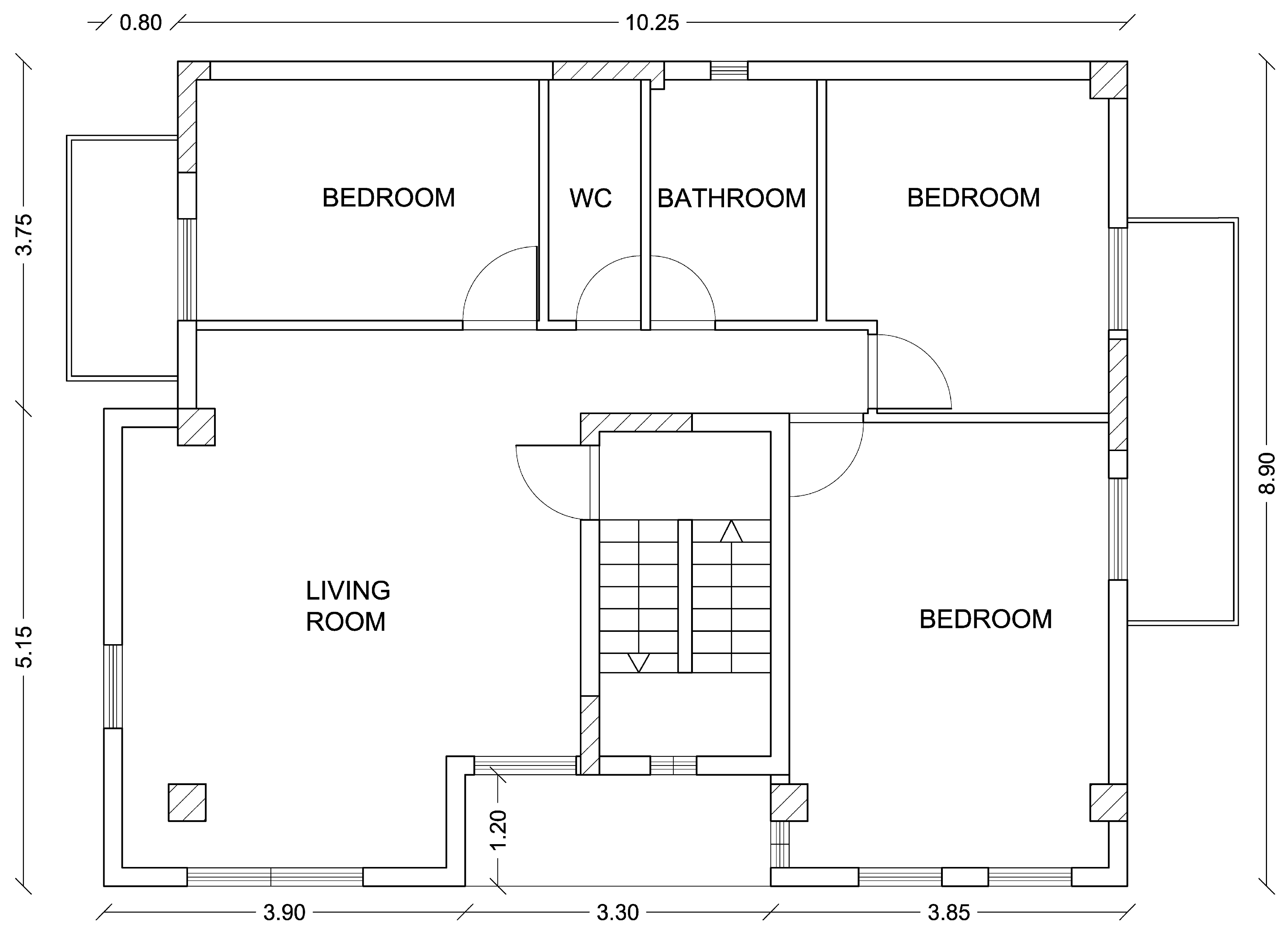
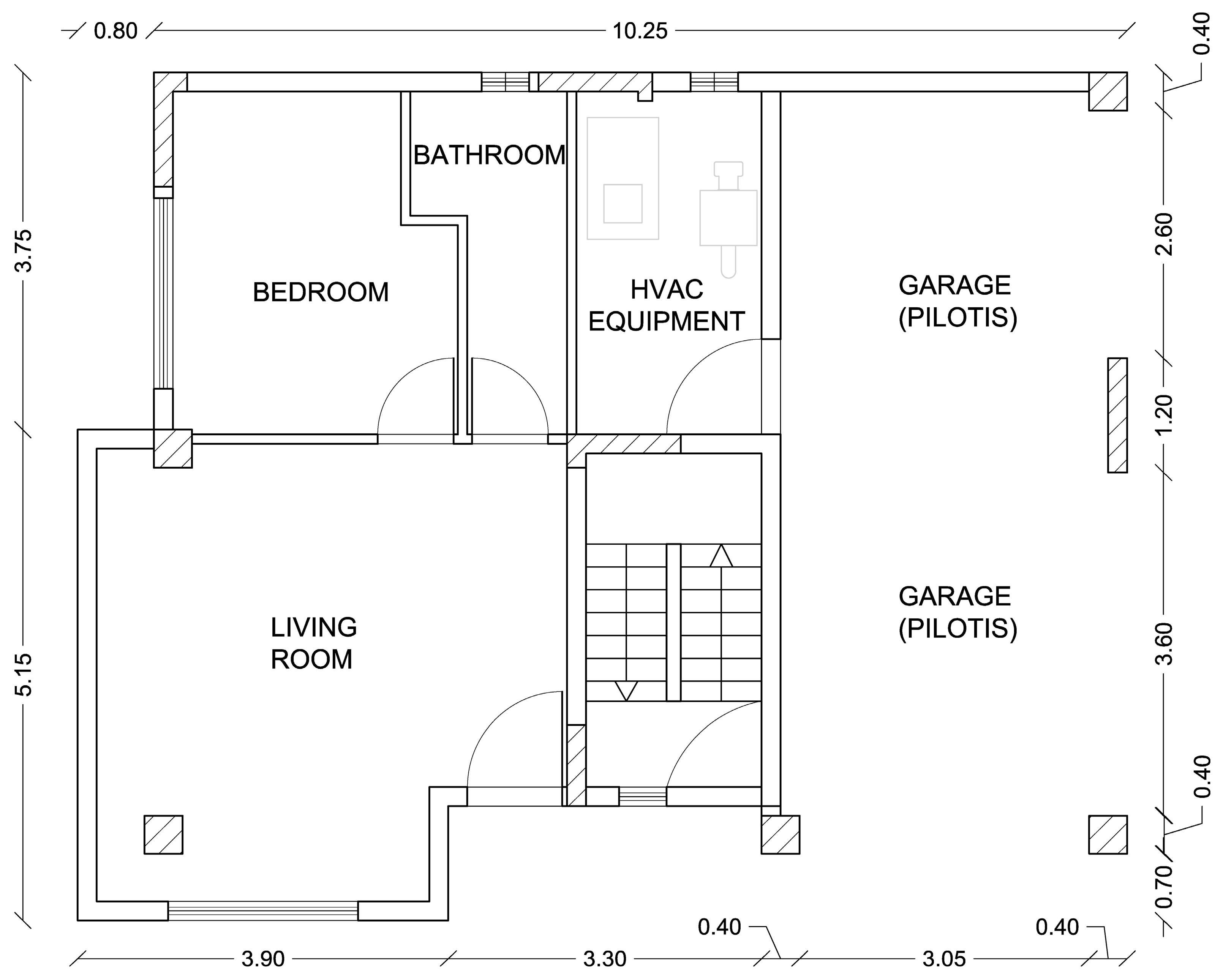
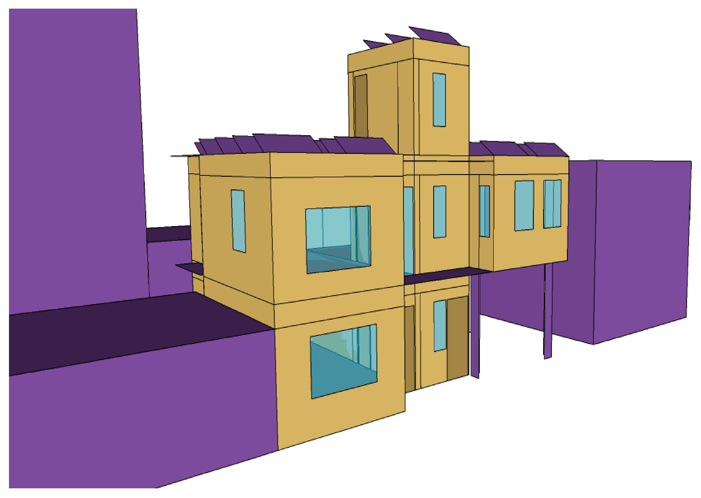
2.1. Case Study Reference Building
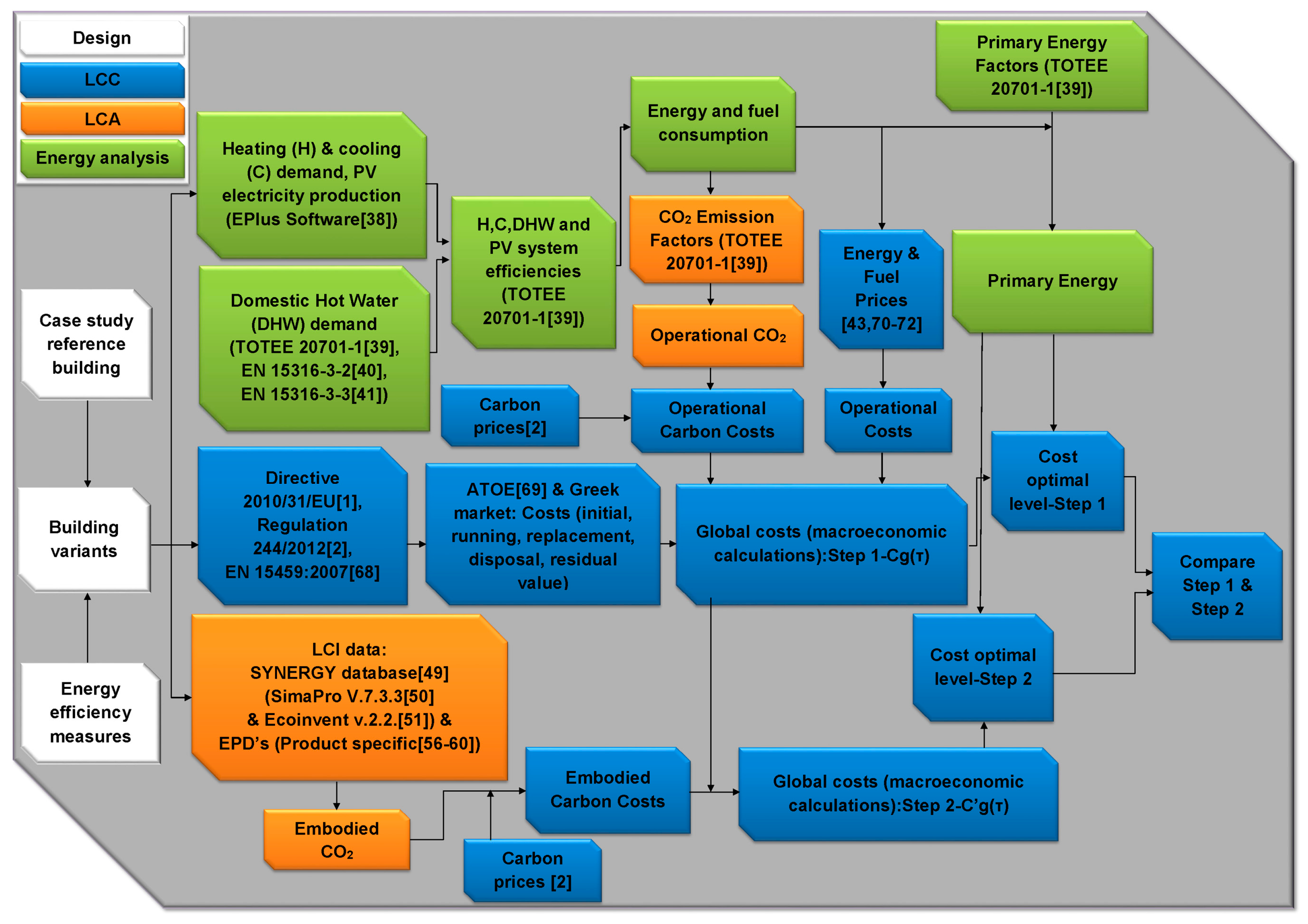
2.2. Analysis
- Energy Analysis: For the quantification of the energy demand for the heating, cooling, domestic hot water and the electricity production, the calculation of the consumption and generation of fuels and electricity and finally the primary energy consumption of the building’s variants.
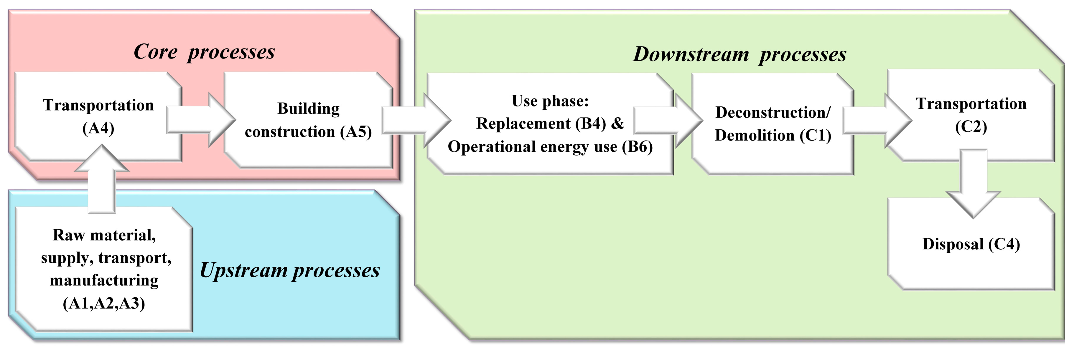
- Life Cycle Assessment (LCA): For the quantification of the embodied impact, through process analysis and for the whole life cycle of the building, in carbon dioxide emissions equivalent.
- Life Cycle Cost (LCC) Analysis: For the calculations of the initial, the running, the replacement, the energy, the carbon and the disposal costs, the residual value and finally the total global costs for the macroeconomic calculations and for both steps of the procedure (Section 2.3 Method).
2.2.1. Energy Analysis
2.2.2. Life Cycle Assessment (LCA)
2.2.3. Life Cycle Cost (LCC) Analysis
2.3. Method
- is the calculation period in years
- is the global cost (referred to the starting year ) over the calculation period in euro
- is the initial investment cost for measure or set of measures j in euro
- is the annual (running, energy and replacement) cost during year i for measure or set of measures j in euro
- is the discount factor for year i based on the discount rate r to be calculated
- is the number of years from the starting period
- r is the real discount rate
- is the residual value of measure or set of measures j at the end of the calculation period (discounted to the starting year τ0) in euro and
- is the carbon cost of measure or set of measures j during year i in euro.
- Step 1. Global cost calculation for the macroeconomic perspective, as defined in the recast of the European Directive 2010/31/EE, the delegated Regulation 244/2012 and the accompanying guidelines.
- Step 2. Global cost calculation for the macroeconomic perspective, with the extension of the emission costs and the consideration of carbon emissions for the whole life cycle of the building.
2.3.1. Step 1
2.3.2. Step 2
- is the global cost (referred to the starting year ) over the calculation period in euro, for the total life cycle assessment, including the embodied and operating carbon costs
- is the carbon cost of measure or set of measures j during year i in euro, from the operation of the building
- is the embodied carbon cost of measure or set of measures j during year i in euro and
- is the carbon cost of measure or set of measures j during year i in euro, from the total life cycle of the building.
2.3.3. Sensitivity Analysis
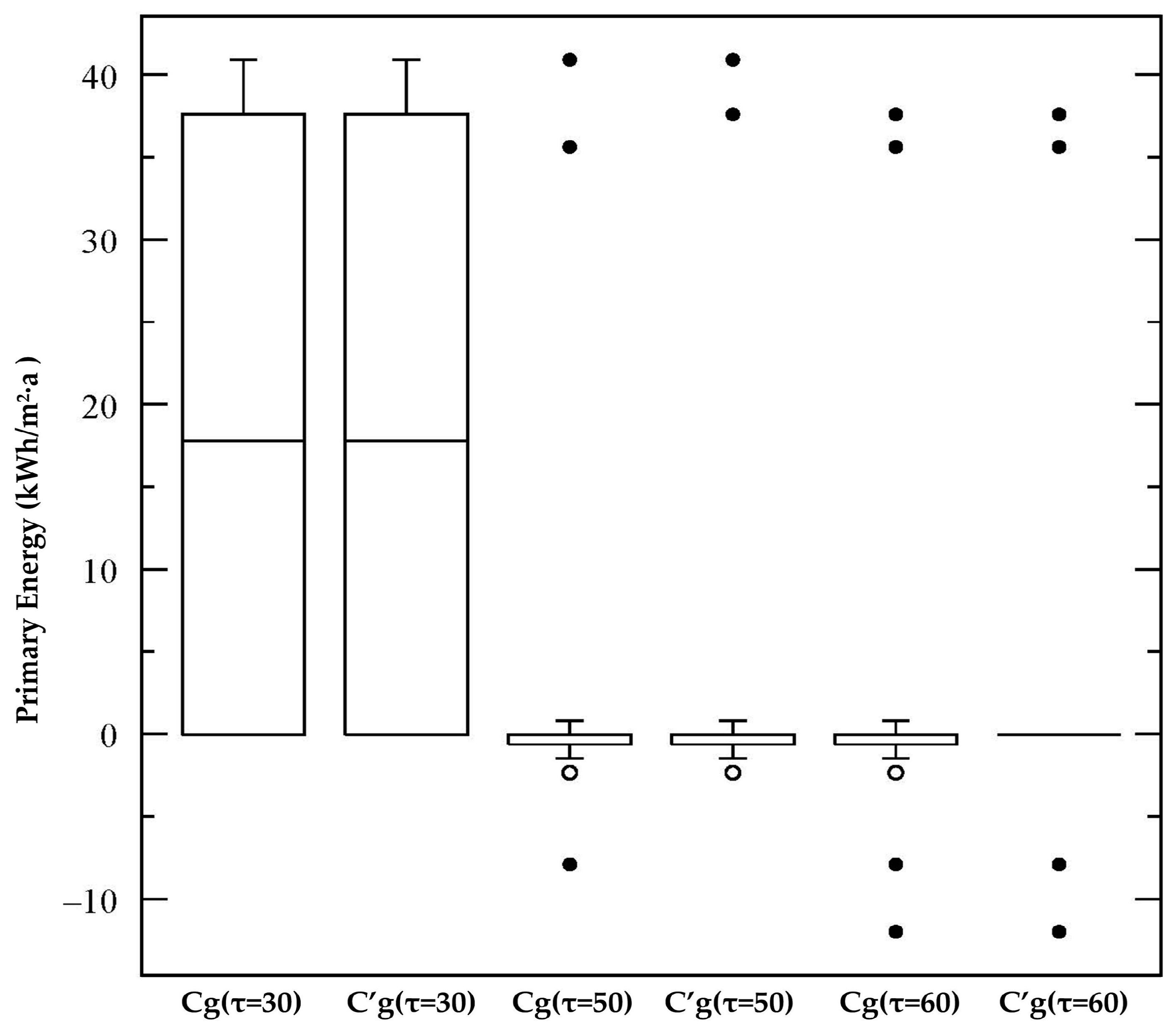
3. Results and Discussion
4. Conclusions
Acknowledgments
Author Contributions
Conflicts of Interest
References
- Directive 2010/31/EU of the European Parliament and of the Council of 19 May 2010 on the Energy Performance of Buildings (Recast). Available online: http://eur-lex.europa.eu/legal-content/EN/TXT/PDF/?uri=CELEX:32010L0031&from=EN (accessed on 15 March 2015).
- Commission Delegated Regulation (EU) No 244/2012 of 16 January 2012 Supplementing Directive 2010/31/EU of the European Parliament and of the Council on the Energy Performance of Buildings by Establishing a Comparative Methodology Framework for Calculating Cost-Optimal Levels of Minimum Energy Performance Requirements for Buildings and Building Elements. Available online: http://eur-lex.europa.eu/legal-content/EN/TXT/PDF/?uri=CELEX:32012R0244&from=EN (accessed on 15 March 2015).
- Guidelines Accompanying Commission Delegated Regulation (EU) No 244/2012 of 16 January 2012 Supplementing Directive 2010/31/EU of the European Parliament and of the Council on the Energy Performance of Buildings by Establishing a Comparative Methodology Framework for Calculating Cost-Optimal Levels of Minimum Energy Performance Requirements for Buildings and Building Elements. Available online: http://eur-lex.europa.eu/legal-content/EN/TXT/PDF/?uri=CELEX:52012XC0419(02)&from=SK (accessed on 15 March 2015).
- Karimpour, M.; Belusko, M.; Xing, K.; Bruno, F. Minimising the life cycle energy of buildings: Review and analysis. Build. Environ. 2014, 73, 106–114. [Google Scholar] [CrossRef]
- Ramesh, T.; Prakash, R.; Shukla, K.K. Life cycle energy analysis of buildings: An overview. Energy Build. 2010, 42, 1592–1600. [Google Scholar] [CrossRef]
- Sartori, I.; Hestnes, A.G. Energy use in the life cycle of conventional and low-energy buildings: A review article. Energy Build. 2007, 39, 249–257. [Google Scholar] [CrossRef]
- Chastas, P.; Theodosiou, T.; Bikas, D. Embodied energy in residential buildings-towards the nearly zero energy building: A literature review. Build. Environ. 2016, 105, 267–282. [Google Scholar] [CrossRef]
- Thiel, C.L.; Campion, N.; Landis, A.E.; Jones, A.K.; Schaefer, L.A.; Bilec, M.M. A materials life cycle assessment of a net-zero energy building. Energies 2013, 6, 1125–1141. [Google Scholar] [CrossRef]
- Cellura, M.; Guarino, F.; Longo, S.; Mistretta, M. Energy life-cycle approach in Net zero energy buildings balance: Operation and embodied energy of an Italian case study. Energy Build. 2014, 72, 371–381. [Google Scholar] [CrossRef]
- Stephan, A.; Crawford, R.H. A multi-scale life-cycle energy and greenhouse- gas emissions analysis model for residential buildings. Archit. Sci. Rev. 2014, 57, 39–48. [Google Scholar] [CrossRef]
- Hernandez, P.; Kenny, P. Development of a methodology for life cycle building energy ratings. Energy Policy 2011, 39, 3779–3788. [Google Scholar] [CrossRef]
- Pombo, O.; Allacker, K.; Rivela, B.; Neila, J. Sustainability assessment of energy saving measures: A multi-criteria approach for residential buildings retrofitting—A case study of the Spanish housing stock. Energy Build. 2016, 116, 384–394. [Google Scholar] [CrossRef]
- Hall, M.; Geissler, A.; Burger, B. Two years of experience with a net zero energy balance—Analysis of the Swiss MINERGIE—A standard. Energy Procedia 2014, 48, 1281–1291. [Google Scholar] [CrossRef]
- BREEAM International New Construction Technical Manual. Available online: http://www.breeam.com/BREEAMInt2013SchemeDocument/#09_materials/mat_01_life_cycle_impacts.htm#kanchor301 (accessed on 26 December 2016).
- The Code for Sustainable Homes Setting the Standard in Sustainability for New Homes. Available online: http://webarchive.nationalarchives.gov.uk/20120919132719/www.communities.gov.uk/documents/planningandbuilding/pdf/codesustainhomesstandard.pdf (accessed on 25 August 2015).
- DGNB Criterion ECO 1.1 Life Cycle Cost. Available online: http://www.dgnb-system.de/en/system/criteria/core14/# (accessed on 25 October 2016).
- BREEAM Green Guide Online Calculator Tool Guidance. Available online: https://www.bre.co.uk/filelibrary/greenguide/PDF/PN284-Green-Guide-Calculator-Guidance-Jan2015.pdf (accessed on 26 December 2016).
- DGNB Criterion ENV 2.1 Life Cycle Assessment Primary Energy. Available online: http://www.dgnb-system.de/en/system/criteria/core14/# (accessed on 25 October 2016).
- International Initiative for a Sustainable Built Environment. Available online: http://www.iisbe.org/sbmethod (accessed on 8 September 2016).
- JSBC Comprehensive Assessment System for Building Environmental Efficiency (CASBEE) for New Construction-Tecnical Manual. Available online: http://www.ibec.or.jp/CASBEE/english/download/CASBEE-BD(NC)e_2014manual.pdf (accessed on 25 August 2015).
- U.S Green Building Council: LEED v4 for Building Design and Construction. Available online: http://www.usgbc.org/resources/leed-v4-building-design-and-construction-current-version (accessed on 10 January 2015).
- DGNB Criterion ENV 1.3 Responsible Procurement. Available online: http://www.dgnb-system.de/en/system/criteria/core14/# (accessed on 25 October 2016).
- BEAM Plus New Buildings and Existing Buildings. Available online: https://www.hkgbc.org.hk/eng/BEAMPlus_NBEB.aspx (accessed on 13 September 2016).
- Green Star Material Calculator Guide. Available online: https://www.google.gr/url?sa=t&rct=j&q=&esrc=s&source=web&cd=1&cad=rja&uact=8&ved=0ahUKEwi05bzT_MXLAhXFlnIKHebfBY4QFggbMAA&url=https%3A%2F%2Fwww.gbca.org.au%2Fuploads%2F239%2F2287%2FGreen%2520Star%2520Material%2520Calculator%2520Guide_v5.pdf&usg=AFQjCNGW60h9OLzZKW_8PMXUh71FJwBuXA&sig2=9SxqqQqTJGAS_M8IHrXiVA&bvm=bv.117218890,d.bGQ (accessed on 16 August 2016).
- Lee, B.; Trcka, M.; Hensen, J.L.M. Embodied energy of building materials and green building rating systems-A case study for industrial halls. Sustain. Cities Soc. 2011, 1, 67–71. [Google Scholar] [CrossRef]
- Chandratilake, S.R.; Dias, W.P.S. Sustainability rating systems for buildings: Comparisons and correlations. Energy 2013, 59, 22–28. [Google Scholar] [CrossRef]
- Andrade, J.; Bragança, L. Sustainability assessment of dwellings—A comparison of methodologies. Civ. Eng. Environ. Syst. 2016, 33, 125–146. [Google Scholar] [CrossRef]
- Suzer, O. A comparative review of environmental concern prioritization: LEED vs other major certification systems. J. Environ. Manag. 2015, 154, 266–283. [Google Scholar] [CrossRef] [PubMed]
- Sesana, M.M.; Salvalai, G. Overview on life cycle methodologies and economic feasibility for nZEBs. Build. Environ. 2013, 67, 211–216. [Google Scholar] [CrossRef]
- International Organization for Standardization. ISO 14040: Environmental Management—Life Cycle Assessment—Principles and Framework; International Organization for Standardization: Geneva, Switzerland, 2006. [Google Scholar]
- International Organization for Standardization. ISO 14044: Environmental Management—Life Cycle Assessment—Requirements and Guidelines; International Organization for Standardization: Geneva, Switzerland, 2006. [Google Scholar]
- International Organization for Standardization. ISO 14025: Environmental Labels and Declarations—Type III Environmental Declarations—Principles and Procedures; International Organization for Standardization: Geneva, Switzerland, 2006. [Google Scholar]
- Overview of Member States Information on NZEBs-Working Version of the Progress Report-Final Report. Available online: https://ec.europa.eu/energy/sites/ener/files/documents/Updated%20progress%20report%20NZEB.pdf (accessed on 15 June 2016).
- Report from the Comission to the European Parliament and the Council-Progress by Member States in Reaching Cost-Optimal Levels of Minimum Energy Performance Requirements. Available online: http://eur-lex.europa.eu/legal-content/EN/TXT/PDF/?uri=CELEX:52016DC0464&from=EN (accessed on 10 January 2017).
- Hellenic Statistical Authority. Available online: http://www.statistics.gr/el/census-buildings-2011 (accessed on 25 August 2015).
- Technical Guide 20701-3: Climatic Data of Greek Regions. Available online: http://portal.tee.gr/portal/page/portal/tptee/totee/TOTEE-20701-3-Final-TEE%203nd%20Edition.pdf (accessed on 13 February 2015).
- Greek Regulation for the Energy Efficiency of Buildings (KENAK). Available online: http://portal.tee.gr/portal/page/portal/tptee/totee/FEK%20407-B-2010%20-%20KENAK.pdf (accessed on 13 February 2015).
- Energy Plus TM. National Renewable Energy Laboratory. Available online: https://energyplus.net/ (accessed on 12 February 2016).
- Technical Guide 20701-1: Descriptive national Specifications for the Calculation of the Energy Efficiency of Buildings and the Energy Efficiency Certificate Auditing. Available online: http://portal.tee.gr/portal/page/portal/tptee/totee/TOTEE-20701-2 Final-%D4%C5%C5%20-%202nd%20edition.pdf (accessed on 13 February 2015).
- Heating Systems in Buildings—Method for Calculation of System Energy Requirements and System Efficiencies-Part 3-2: Domestic Hot Water Systems, Distribution. Available online: http://www.cres.gr/greenbuilding/PDF/prend/set3/WI_11_TC-approval_version_prEN_15316-3-2_Domestic_hot_water_-_Distribution.pdf (accessed on 20 March 2017).
- Heating Systems in Buildings-Method for Calculation of System Energy Requirements and System Efficiencies-Part 3-3: Domestic Hot Water Systems, Generation. Available online: http://www.cres.gr/greenbuilding/PDF/prend/set3/WI_11_TC-approval_version_prEN_15316-3-3_Domestic_hot_water_-_Generation.pdf (accessed on 20 March 2017).
- Droutsa, K.G.; Kontoyiannidis, S.; Dascalaki, E.G.; Balaras, C.A. Mapping the energy performance of hellenic residential buildings from EPC (energy performance certificate) data. Energy 2016, 98, 284–295. [Google Scholar] [CrossRef]
- PV Installations (≤ 10 kW) in Buildings. Available online: http://www.desmie.gr/ape-sithya/adeiodotiki-diadikasia-kodikopoiisi-nomothesias-ape/periechomena/mikra-fotoboltaika-10-kw-se-ktiria/ (accessed on 24 January 2017).
- Martinopoulos, G.; Papakostas, K.T.; Papadopoulos, A.M. Comparative analysis of various heating systems for residential buildings in Mediterranean climate. Energy Build. 2016, 124, 79–87. [Google Scholar] [CrossRef]
- Giama, E.; Papadopoulos, A.M. Assessment tools for the environmental evaluation of concrete, plaster and brick elements production. J. Clean. Prod. 2015, 99, 75–85. [Google Scholar] [CrossRef]
- Sustainability of Construction Works-Assessment of Environmental Performance of Buildings-Calculation Method. Available online: https://www.en-standard.eu/csn-en-15978-sustainability-of-construction-works-assessment-of-environmental-performance-of-buildings-calculation-method/ (accessed on 20 March 2017).
- Sustainability of Construction Works. Environmental Product Declarations-Core Rules for the Product Category of Construction Products. Available online: https://www.en-standard.eu/csn-en-15804-a1-sustainability-of-construction-works-environmental-product-declarations-core-rules-for-the-product-category-of-construction-products/ (accessed on 20 March 2017).
- CML-IA Database. Available online: https://www.universiteitleiden.nl/en/research/research-output/science/cml-ia-characterisation-factors (accessed on 25 March 2016).
- SYNERGY. Research and Development of a System of High Energy-Efficient Building Elements, under Integrated Protection Criteria and Life-Cycle Design Aspects, through the SYNERGASIA 2011; SYNERGY: Thessaloniki, Greece, 2014. [Google Scholar]
- Sima Pro Software v.7.3.3. Available online: https://www.pre-sustainability.com/simapro (accessed on 10 May 2014).
- Ecoinvent Database v.2.2. Available online: http://www.ecoinvent.org/database/older-versions/ecoinvent-version-2/ecoinvent-version-2.html (accessed on 10 May 2014).
- Andersen, S.; Dinesen, J.; Hjort Knudsen, H.; Willendrup, A. Livscyklus-Baseret Bygningsprojektering (Life-Cycle-Based Building Design, Energy and Environment Model, Calculating Tool and Database); Danish Building Research Institute: Hørsholm, Denmark, 1993. [Google Scholar]
- Koubogiannis, D.; Nouhou, C. How much Energy is Embodied in your Central Heating Boiler? IOP Conf. Ser. Mater. Sci. Eng. 2016, 161, 1–9. [Google Scholar] [CrossRef]
- Piroozfar, P.; Pomponi, F.; Farr, E.R.P. Life cycle assessment of domestic hot water systems: A comparative analysis. Int. J. Constr. Manag. 2016, 16, 109–125. [Google Scholar] [CrossRef]
- International EPD System: Environmental Product Declaration. Available online: http://www.environdec.com/ (accessed on 9 January 2016).
- EPD Flat Glass, Toughened Safety Glass and Laminated Safety Glass. Available online: http://www.euroglas.com/fileadmin/content/euroglas/Deutsch/Service/Zertifizierungen/EPD_FB_ESG_VSG_Float_EN.pdf (accessed on 25 October 2016).
- Iplus|Planibel Low-e the Range of AGC Glasses with Thermal Insulation. Available online: http://www.agcnederland.nl/docs/EPD%20AGC%20Iplus.pdf (accessed on 25 October 2016).
- EPD Polisan Exelans Macro External Paint. Available online: http://yesilmalzemeler.com.tr/Content/urun-sertifikasi-polisan-exelans-macro-7270013690.PDF (accessed on 25 January 2017).
- EPD Polisan Natura Ambians Internal Paint. Available online: http://environdec.com/en/Detail/epd739 (accessed on 25 January 2017).
- EPD-Hot-Dip Galvanized Products. Available online: http://cdn.ruukki.com/docs/default-source/b2b-documents/epd/en-epd-rc-hot-dip-galvanised.pdf?sfvrsn=20 (accessed on 25 January 2017).
- Adalberth, K. Energy use during the Life cycle of Single Unit Dwellings: Examples. Build. Environ. 1997, 32, 321–329. [Google Scholar] [CrossRef]
- Blengini, G.A. Life cycle of buildings, demolition and recycling potential: A case study in Turin, Italy. Build. Environ. 2009, 44, 319–330. [Google Scholar] [CrossRef]
- Blengini, G.A.; Di Carlo, T. The changing role of life cycle phases, subsystems and materials in the LCA of low energy buildings. Energy Build. 2010, 42, 869–880. [Google Scholar] [CrossRef]
- Chen, T.Y.; Burnett, J.; Chau, C.K. Analysis of embodied energy use in the residential building of Hong Kong. Energy 2001, 26, 323–340. [Google Scholar] [CrossRef]
- Bundesministerium für Umwelt, Naturschutz, Bau und Reaktorsicherheit (BMUB). Nutzungsdauern von Bauteilen, Datenbank Zwischenauswertung; German Federal Ministry for the Environment, Nature Conservation, Building and Nuclear Safety: Berlin, Germany, 2008. [Google Scholar]
- International Organization for Standardization. ISO 15686: Buildings And Constructed Assets—Service-Life Planning—Part 5: Life-Cycle Costing; International Organization for Standardization: Geneva, Switzerland, 2008. [Google Scholar]
- Product Category Rules according to ISO 14025:2006 Product Group-2014:02. Available online: http://environdec.com/en/PCR/Detail/?show_login=true&error=failure&Pcr=5950 (accessed on 28 May 2015).
- Energy Efficiency for Buildings—Standard Economic Evaluation Procedure For Energy Systems in Buildings. Available online: http://www.cres.gr/greenbuilding/PDF/prend/set4/WI_29_TC-approval_version_prEN_15459_Data_requirements.pdf (accessed on 20 March 2017).
- ATOE-Descriptive Bills of Building Construction Works. Available online: http://www.sate.gr/html/timologia.aspx (accessed on 16 January 2016).
- Natural Gas Prices for Household Consumers. Available online: http://ec.europa.eu/eurostat/statistics-explained/index.php/Natural_gas_price_statistics#Natural_gas_prices_for_household_consumers (accessed on 10 January 2017).
- Electricity Prices for Household Consumers. Available online: http://ec.europa.eu/eurostat/statistics-explained/index.php/Energy_price_statistics#Electricity_prices_for_household_consumers (accessed on 10 January 2017).
- Heating Oil Prices. Available online: http://www.popek.gr/index.php/el/times-kafsimon/home (accessed on 10 January 2017).
- Indicator of New Building Construction Costs. Available online: http://www.statistics.gr/el/statistics/-/publication/DKT63/ (accessed on 25 August 2015).
- Dahlstrøm, O.; Sørnes, K.; Eriksen, S.T.; Hertwich, E.G. Life cycle assessment of a single-family residence built to either conventional- or passive house standard. Energy Build. 2012, 54, 470–479. [Google Scholar] [CrossRef]
- Syngros, G.; Balaras, C.A.; Koubogiannis, D.G. Embodied CO2 Emissions in Building Construction Materials of Hellenic Dwellings. Proced. Environ. Sci. 2017, 38, 500–508. [Google Scholar] [CrossRef]
- Hammond, G.; Jones, C. Inventory of Carbon and Energy: ICE; University of Bath: Bath, UK, 2008. [Google Scholar]


| Building Features | Value |
|---|---|
| Total area (m2) | 191.10 |
| Heated (reference) area (m2) | 123.75 |
| Non-heated area (m2) | 34.86 |
| Pilotis-open area (m2) | 32.49 |
| External wall area (m2) | 210.11 |
| Fenestration area (m2) | 31.37 |
| Window to wall ratio (%) | 14.93 |
| Energy Demand | (kWh/m2∙a *) |
|---|---|
| Heating | 53.59 |
| Cooling | 33.27 |
| Domestic Hot Water | 30.30 |
| Total | 117.16 |
| Building Element | Min U-Value (W/m2∙K) | Reference U-Value (W/m2∙K) | Max U-Value (W/m2∙K) |
|---|---|---|---|
| Wall of reinforced concrete | 0.866 | 0.387 | 0.233 |
| Masonry of bricks | 0.685 | 0.346 | 0.217 |
| Flat roof | 0.691 | 0.348 | 0.218 |
| Ground floor | 0.742 | 0.613 | 0.402 |
| Floor over pilotis | 0.825 | 0.379 | 0.230 |
| Floor in contact with non-heated area | 0.726 | 0.601 | 0.397 |
| Wall of reinforced concrete in contact with non-heated area | 0.800 | 0.651 | 0.418 |
| Masonry of bricks in contact with non-heated area | 0.663 | 0.558 | 0.377 |
| Window Glazing | Uw-Value (W/m2∙K) |
|---|---|
| W0: Reference (4/6air/4) | 2.74 |
| W1: 6/12air/6 | 2.56 |
| W2: 6/12argon/6 | 2.44 |
| W3: low-e 6/12air/6 | 1.95 |
| W4: 6/12air/6/12air/6 | 1.88 |
| W5: 6/12argon/6/12argon/6 | 1.78 |
| W6: low-e 6/12argon/6 | 1.76 |
| W7: low-e 6/12air/6/12air/6 | 1.61 |
| W8: low-e 6/12argon/6/12argon/6 | 1.47 |
| Difference in Total Energy Demand (kWh/m2∙a) | Window Glazing | |||||||
|---|---|---|---|---|---|---|---|---|
| Insulation Thickness (m) | W1 | W2 | W3 | W4 | W5 | W6 | W7 | W8 |
| 0.03 | 30.51 | 29.96 | 25.49 | 26.41 | 25.86 | 24.11 | 23.48 | 22.48 |
| 0.04 | 20.28 | 19.74 | 15.02 | 16.04 | 15.49 | 13.63 | 12.93 | 11.93 |
| 0.05 | 13.30 | 12.76 | 7.82 | 8.95 | 8.40 | 6.45 | 5.66 | 4.67 |
| 0.06 | 8.17 | 7.64 | 2.54 | 3.74 | 3.20 | 1.17 | 0.33 | −0.66 |
| 0.07 | 3.13 | 2.59 | −2.69 | −1.41 | −1.95 | −4.06 | −5.00 | −5.98 |
| 0.08 | 0.01 | −0.53 | −5.89 | −4.58 | −5.13 | −7.27 | −8.25 | −9.22 |
| 0.09 | −3.31 | −3.85 | −9.33 | −7.97 | −8.52 | −10.71 | −11.72 | −12.69 |
| 0.10 | −5.29 | −5.82 | −11.37 | −9.99 | −10.54 | −12.75 | −13.79 | −14.77 |
| 0.12 | −9.31 | −9.84 | −15.52 | −14.09 | −14.64 | −16.91 | −17.99 | −18.96 |
| 0.14 | −12.22 | −12.75 | −18.53 | −17.06 | −17.60 | −19.91 | −21.04 | −22.01 |
| Installed Power (kW) | Number of Modules | PV Area (m2) | Electricity Production (kWh/a) |
|---|---|---|---|
| 1.0 | 4.0 | 6.6 | 1420.89 |
| 1.5 | 6.0 | 9.9 | 2097.31 |
| 2.0 | 8.0 | 13.2 | 2785.59 |
| 2.5 | 10.0 | 16.5 | 3444.97 |
| 3.0 | 12.0 | 19.8 | 4141.71 |
| 3.5 | 14.0 | 23.1 | 4812.77 |
| 4.0 | 16.0 | 26.4 | 5471.66 |
| Scenario | System | Fuel | Efficiency | Primary Energy Factor |
|---|---|---|---|---|
| 1 | Heating | Gas | 0.812 | 1.05 |
| Cooling | Electricity | 2.790 | 2.90 | |
| DHW | Gas | 0.794 | 1.05 | |
| Production | Electricity (PV) | 0.960 (inverter) | 2.90 | |
| 2 | Heating | Oil * | 0.812 | 1.10 |
| Cooling | Electricity * | 2.790 | 2.90 | |
| DHW | Oil * | 0.794 | 1.10 | |
| Production | Electricity (PV) | 0.960 (inverter) | 2.90 | |
| 3 | Heating | Electricity | 2.980 | 2.90 |
| Cooling | Electricity | 2.790 | 2.90 | |
| DHW | Electricity | 0.980 | 2.90 | |
| Production | Electricity (PV) | 0.960 (inverter) | 2.90 |
| Materials & Components | Unit | Quantity (min/max) 1 | Transportation A4/C2 (km) 2 | Reference Service Life (years) | Waste Factor (%) |
|---|---|---|---|---|---|
| Plaster [49] | kg | 37,581.48 | 20/25 | 40 | 10 |
| Mortar [49] | kg | 5212.20 | 20/25 | 40 | 10 |
| Internal paint [59] | kg | 241.89 | 20/25 | 10 | 7 |
| External paint [58] | kg | 212.77 | 20/25 | 10 | 7 |
| Concrete [49] | kg | 224,807.94 | 20/25 | 100 | 10 |
| Brick [49] | kg | 61,797.24 | 15/25 | 90 | 10 |
| Glass fiber [49] | kg | 41.67 | 20/25 | 30 | 7 |
| XPS [49] | kg | 355.54/1466.18 | 70/25 | 40 | 7 |
| Adhesives [49] | kg | 1522.69 | 20/25 | 50 | 0 |
| Steel (reinforcing) [49] | kg | 9036.78 | 30/25 | 100 | 7 |
| HDPE [49] | kg | 57.51 | 20/25 | 30 | 7 |
| Gravel [49] | kg | 15,843.60 | 40/25 | 80 | 10 |
| Poor concrete [49] | kg | 17,807.04 | 20/25 | 80 | 10 |
| Ceramic tiles [49] | kg | 2629.82 | 1400/25 | 50 | 10 |
| Bitumen [49] | kg | 601.72 | 20/25 | 30 | 7 |
| Argon [49] | kg | 0.00/0.99 | 8/25 | 25 | 0 |
| PVC profile [49] | kg | 137.17 | 8/25 | 50 | 10 |
| Flat glass [56] | kg | 686.50/1028.25 | 8/25 | 25 | 0 |
| Glass (low-e) [57] | kg | 0.00/342.75 | 8/25 | 25 | 0 |
| Wood (Oak) [49] | kg | 1130.40 | 30/25 | 50 | 7 |
| MDF [49] | kg | 343.80 | 30/25 | 60 | 7 |
| PV panels [49] | kg | 0.00/319.52 | 2000/25 | 30 | 7 |
| Heating & DHW system (Scen. 3 1 & 2) [49,53] | kg | 345.00/465.00 | 700/25 | 25 | 6 |
| Electronics [49] | kg | 0.00/85.00 | 2000/25 | 15 | 6 |
| Galvanized steel [60] | kg | 0.00/160.00 | 30/25 | 40 | 5 |
| Inverter [49] | kg | 0.00/37.00 | 2000/25 | 15 | 5 |
| Cooling System (Scen. 1, 2, 3) [49] | kg | 131.09 | 2000/25 | 20 | 10 |
| Heating & DHW system (Scen. 3) [54] | kg | 251.09 | 700/25 | 25 | 6 |
| Demolition & Site restoration [49] | m3 | 591.74/629.24 | Ν/Α/Ν/Α 4 | Ν/Α | Ν/Α |
| Electricity(A5) 5 [52] | kWh | 16,938.00 | Ν/Α/Ν/Α | Ν/Α | Ν/Α |
| Fuel | CO2 Emission Factor |
|---|---|
| Gas | 0.196 |
| Oil | 0.264 |
| Electricity | 0.989 |
| Cost Category | Cost Type |
|---|---|
| Initial | Design |
| Material | |
| Transportation to the construction site | |
| Energy for construction | |
| Labour | |
| Recurring | Running |
| Replacement | |
| Energy | |
| Emission (carbon) | |
| Disposal | Demolition |
| Transportation to landfill | |
| Landfill disposal |
| Parameter | Value |
|---|---|
| Calculation period (τ) | 30 years |
| Starting year () | 2016 |
| Discount rate () | 3.0% |
| Gas price | 0.050€ |
| Oil price | 0.053€ |
| Electricity price | 0.1557€ |
| Feed-in tariff | 0.115€ |
| Evolution of energy prices | 2.8% |
| Carbon price, year 2020 | 16.5€ |
| Carbon price, year 2025 | 20.0€ |
| Carbon price, year 2030 | 36.0€ |
| Carbon price, year 2035 | 50.0€ |
| Carbon price, year 2040 | 52.0€ |
| Carbon price, year 2045 | 51.0€ |
| Carbon price, year 2050 | 50.0€ |
| Parameter | Sensitivity Value | ||||||||
| Discount rate | 2.0% | 3.0% * | 4.0% | ||||||
| Evolution of energy prices | 1.87% | 2.8% * | 4.2% | ||||||
| Evolution of construction and labour prices | 0.0% * | −2.32% | |||||||
| Calculation period | 30 years * | 50 years | 60 years | ||||||
| Evolution of Carbon Prices | |||||||||
| 2020 | 2025 | 2030 | 2035 | 2040 | 2045 | 2050 | |||
| 16.5€ * | 20.0€ | 36.0€ | 50.0€ | 52.0€ | 51.0€ | 50.0€ | |||
| 25.0€ | 38.0€ | 60.0€ | 64.0€ | 78.0€ | 115.0€ | 190.0€ | |||
| 25.0€ | 34.0€ | 51.0€ | 53.0€ | 64.0€ | 92.0€ | 147.0€ | |||
| Scenario | Values | ||
|---|---|---|---|
| Evolution of Energy Prices (%) | Evolution of Construction Costs (%) | Evolution of Carbon Prices (€) | |
| Re 1 | 2.80 | 0.00 | 16.5–50.0 |
| Lpr 2 | 2.80 | −2.32 | 16.5–50.0 |
| HCO2 3 | 2.80 | 0.00 | 25.0–190.0 |
| MCO2 4 | 2.80 | 0.00 | 25.0–147.0 |
| Len 5 | 1.87 | 0.00 | 16.5–50.0 |
| Hen 6 | 4.20 | 0.00 | 16.5–50.0 |
| Step 1 | |||||||
| Discount Rate (%) | |||||||
| 2.0% | 3.0% | 4.0% | |||||
| Scenarios | PE 1 (kWh/m2∙a) | 2 (€) | PE (kWh/m2∙a) | (€) | PE (kWh/m2∙a) | (€) | |
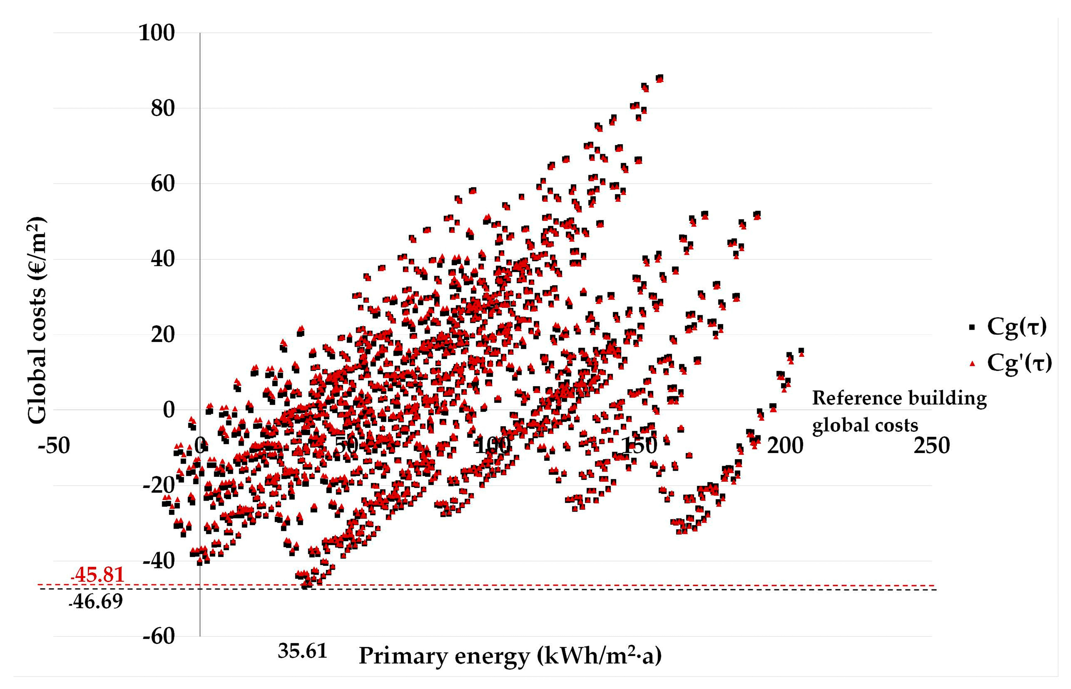
| Scenario | Re | −0.06 | −57.82 | 35.61 | −46.69 | 40.91 | −40.01 |
| Lpr | −0.06 | −58.17 | 35.61 | −46.99 | 40.91 | −40.27 | |
| HCO2 | −0.06 | −89.67 | −0.06 | −67.33 | 37.60 | −50.93 | |
| MCO2 | −0.06 | −78.01 | −0.06 | −57.77 | 37.60 | −47.10 | |
| Len | 35.61 | −61.16 | 37.60 | −51.92 | 40.91 | −45.03 | |
| Hen | −0.06 | −66.33 | −0.06 | −47.67 | −0.06 | −32.52 | |
| Step 2 | |||||||
| Discount Rate (%) | |||||||
| 2.0% | 3.0% | 4.0% | |||||
| Scenarios | PE (kWh/m2∙a) | 3 (€) | PE (kWh/m2∙a) | (€) | PE (kWh/m2∙a) | (€) | |
| Scenario | Re | −0.06 | −56.71 | 35.61 | −45.81 | 40.91 | −39.44 |
| Lpr | −0.06 | −57.06 | 35.61 | −46.11 | 40.91 | −39.71 | |
| HCO2 | −0.06 | −87.91 | −0.06 | −65.64 | 37.60 | −49.83 | |
| MCO2 | −0.06 | −76.31 | −0.06 | −57.77 | 37.60 | −45.99 | |
| Len | 35.61 | −60.28 | 37.60 | −51.17 | 40.91 | −44.47 | |
| Hen | −0.06 | −65.22 | −0.06 | −47.67 | −0.06 | −31.46 | |
| Step 1 | |||||||
| Discount Rate (%) | |||||||
| 2.0% | 3.0% | 4.0% | |||||
| Scenarios | PE 1 (kWh/m2∙a) | 2 (€) | PE (kWh/m2∙a) | (€) | PE (kWh/m2∙a) | (€) | |
| Scenario | Re | −0.06 | −85.02 | −0.06 | −57.35 | −0.06 | −36.85 |
| Lpr | −2.35 | −89.41 | −0.06 | −60.06 | −0.06 | −38.79 | |
| HCO2 | −2.35 | −185.50 | −0.06 | −130.37 | −0.06 | −91.04 | |
| MCO2 | −0.06 | −152.56 | −0.06 | −106.57 | −0.06 | −73.41 | |
| Len | −0.06 | −73.05 | 35.61 | −52.72 | 40.91 | −45.35 | |
| Hen | −7.91 | −113.69 | −2.35 | −76.51 | −0.06 | −50.42 | |
| Step 2 | |||||||
| Discount Rate (%) | |||||||
| 2.0% | 3.0% | 4.0% | |||||
| Scenarios | PE (kWh/m2∙a) | 3 (€) | PE (kWh/m2∙a) | (€) | PE (kWh/m2∙a) | (€) | |
| Scenario | Re | −0.06 | −82.34 | −0.06 | −55.14 | −0.06 | −34.98 |
| Lpr | −2.35 | −86.57 | −0.06 | −57.85 | −0.06 | −36.92 | |
| HCO2 | −2.35 | −178.90 | −0.06 | −125.49 | −0.06 | −87.13 | |
| MCO2 | −0.06 | −147.31 | −0.06 | −102.41 | −0.06 | −70.01 | |
| Len | −0.06 | −70.36 | 37.60 | −50.92 | 40.91 | −44.17 | |
| Hen | −2.35 | −110.80 | −2.35 | −74.17 | −0.06 | −48.54 | |
| Step 1 | |||||||
| Discount Rate (%) | |||||||
| 2.0% | 3.0% | 4.0% | |||||
| Scenarios | PE 1 (kWh/m2∙a) | 2 (€) | PE (kWh/m2∙a) | (€) | PE (kWh/m2∙a) | (€) | |
| Scenario | Re | −0.06 | −119.99 | −0.06 | −77.71 | −0.06 | −48.78 |
| Lpr | −11.97 | −128.15 | −0.06 | −81.15 | −0.06 | −51.17 | |
| HCO2 | −2.35 | −245.80 | −0.06 | −165.46 | −0.06 | −111.60 | |
| MCO2 | −0.06 | −205.03 | −0.06 | −137.13 | −0.06 | −91.32 | |
| Len | −0.06 | −101.38 | 35.61 | −69.37 | 37.60 | −55.04 | |
| Hen | −11.97 | −181.33 | −7.91 | −109.35 | −0.06 | −68.66 | |
| Step 2 | |||||||
| Discount Rate (%) | |||||||
| 2.0% | 3.0% | 4.0% | |||||
| Scenarios | PE (kWh/m2∙a) | 3 (€) | PE (kWh/m2∙a) | (€) | PE (kWh/m2∙a) | (€) | |
| Scenario | Re | −0.06 | −117.29 | −0.06 | −75.49 | −0.06 | −46.90 |
| Lpr | −7.91 | −124.29 | −0.06 | −78.93 | −0.06 | −49.29 | |
| HCO2 | −0.06 | −239.09 | −0.06 | −160.54 | −0.06 | −107.66 | |
| MCO2 | −0.06 | −199.73 | −0.06 | −132.94 | −0.06 | −87.90 | |
| Len | −0.06 | −98.68 | 35.61 | −67.41 | 37.60 | −53.59 | |
| Hen | −11.97 | −176.88 | −7.91 | −106.33 | −0.06 | −68.66 | |
© 2017 by the authors. Licensee MDPI, Basel, Switzerland. This article is an open access article distributed under the terms and conditions of the Creative Commons Attribution (CC BY) license (http://creativecommons.org/licenses/by/4.0/).
Share and Cite
Chastas, P.; Theodosiou, T.; Kontoleon, K.J.; Bikas, D. The Effect of Embodied Impact on the Cost-Optimal Levels of Nearly Zero Energy Buildings: A Case Study of a Residential Building in Thessaloniki, Greece. Energies 2017, 10, 740. https://doi.org/10.3390/en10060740
Chastas P, Theodosiou T, Kontoleon KJ, Bikas D. The Effect of Embodied Impact on the Cost-Optimal Levels of Nearly Zero Energy Buildings: A Case Study of a Residential Building in Thessaloniki, Greece. Energies. 2017; 10(6):740. https://doi.org/10.3390/en10060740
Chicago/Turabian StyleChastas, Panagiotis, Theodoros Theodosiou, Karolos J. Kontoleon, and Dimitrios Bikas. 2017. "The Effect of Embodied Impact on the Cost-Optimal Levels of Nearly Zero Energy Buildings: A Case Study of a Residential Building in Thessaloniki, Greece" Energies 10, no. 6: 740. https://doi.org/10.3390/en10060740