Annual Assessment of Large-Scale Introduction of Renewable Energy: Modeling of Unit Commitment Schedule for Thermal Power Generators and Pumped Storages

Abstract

The fast-increasing introduction of renewable energy sources (RESes) leads to some problems in electrical power network due to fluctuating generated power. A power system must be operated with provision of various reserve powers like governor free capacity, load frequency control and spinning reserve. Therefore, the generator’s schedule (unit commitment schedule) should include the consideration of the various power reserves. In addition, it is necessary to calculate the annual operational costs of electric power systems by solving the unit commitment per week of thermal power generators and pumped storages in order to compare and examine the variance of the operational costs and the operating ratio of the generators throughout the year. This study proposes a novel annual analysis for the thermal power generator and pumped storages under a massive introduction of RESes. A weekly unit commitment schedule (start/stop planning) for thermal power generator and pumped storages has been modeled and calculated for one year evaluation. To solve the generator start/stop planning problem, Tabu search and interior point methods are adopted to solve the operation planning for thermal power generators and the output decision for pumped storages, respectively. It is demonstrated that the proposed method can analyze a one-year evaluation within practical time. In addition, by assuming load frequency control (LFC) constraints to cope with photovoltaic (PV) output fluctuations, the impact of the intensity of LFC constraints on the operational cost of the thermal power generator has been elucidated. The increment of the operational cost of the power supply with increasing PV introduction amount has been shown in concrete terms.

1. Introduction

Due to increased awareness of environmental issues in recent years and constraints on the CO₂ emissions that accompany the use of fossil fuels, expectations for power generation by renewable energy sources (RESes) have increased [1,2]. In case of Japan, among RESes, the adoption of photovoltaics (PVs) and wind turbines (WTs) has rapidly increased following the issuance of feed-in tariff (FIT) in July 2012 [3]. As the end of 2015, over 25 GW of these RESes have been introduced throughout Japan [4], and vigorous efforts are underway to achieve the Japanese government’s PV2030+ goal [5], instituted before the Tohoku great earthquake (11 March 2011), on an accelerated schedule.

However, as PVs and WTs use natural energy as their primary energy source, their output fluctuates. It has therefore been pointed out that PVs and WTs could have a negative impact on the stable operation of a power system [6]. If the output of RESes is unrestrained in the near future in regions such as Hokkaido, Tohoku, and Kyushu as the introduction of PVs and WTs expands, then this could pose a legitimate issue for the power system [4]. One growing concern with the expanded use of RESes is the decrease in their output suppression [7]. Also, given the instability of RES output, when policies for power-system operation are formulated during the large-scale implementation of RESes, then the constraints on load frequency control (LFC) and governor-free system operation must be explicitly taken into account.

On the other hand, as large scale energy storage, pumped storage has been massively adopted in Japan to balance its electricity supply and demand, therefore the high quality of electricity can be maintained. At the end of 2009, the total capacity of pumped storages in Japan was about 25 GW, which represents over 8.5% of installed domestic power generation capacity [8] and is almost equal to 25% of the world total pumped-storage capacity. In addition, pumped storage has several advantages and characteristics including lower cost, applicability for large scale, and possibility for seasonal storage [9]. In addition, pumped storages can act as both supply and demand depending on the grid conditions. Other possible energy storage methods include batteries, hydrogen [10,11], and electric vehicles [12], however they face some economic and technical challenges for large scale application. Optimal and advanced utilization of pumped storage is demanded in the future as the share of RESs increases.

Numerous evaluations of power facility plans spanning several years to several decades [13,14,15,16,17,18] and considerable research on the formulation of power generation operation plans lasting one day to one week have been previously conducted [19]. Komiyama and Fujii [13] have studied the model for the mixed power generation in Japan considering the fluctuating output from both PVs and WTs using linear programming. Unfortunately, the linear programming method is considered unsuitable for finding the solution of non-linear problems, such as power loss, weather conditions, fuel cost, population, and economic activities [20,21]. Therefore, the application of linear modeling in power system results in lower accuracy and it is also difficult to evaluate its validity with the real problems [22]. In addition, Aihara and Yokoyama [16] developed an operation scheduling method to simulate the Japanese weekly demand and supply considering large introduction of PV using dynamic programming. Unfortunately, dynamic programming faces some problems including the dimensionality, especially in the case of large-scale system [23].

In order to conduct a comparative study of changes in operational costs and generator operation rates throughout a year, weekly operating plans for thermal power generator and hydroelectric power generator, especially pumped storage, must be formulated, and annual operating expenses must be calculated. Therefore, in order to perform year-round evaluations of power operation during the large-scale introduction of RESes, this study focus on the modeling of weekly-based operation plans of thermal power generators and pump storages throughout a year. A variety of power generators included in the modeling of this proposed method are thermal power plants (oil, coal, LNG, combined cycle (CC)), hydroelectric power plants (pump storages, dams, inflow), nuclear power plants, and RES generators (geothermal plants, PVs).

In addition, to achieve more definitive results of the unit commitment scheduling for thermal power generators and pumped storages, Tabu search and interior point method are adopted to calculate the operation plan for thermal power generators and pumped storages, respectively. Tabu search is currently one of the most effective methods for finding near-optimal solutions to combinatorial optimization problems [24]. This method emphasizes on the intelligent search with concept of neighborhood becomes one of the key factor. On the other hand, the interior point method has been used broadly in electric power systems to solve the optimization problems. It is capable of giving a solution for both linear and nonlinear convex optimization problems. Furthermore, the application of both Tabu search and interior point methods are expected to be able to result in more optimal operating conditions which have high compatibility with the actual operation.

2. Generator Operation Model

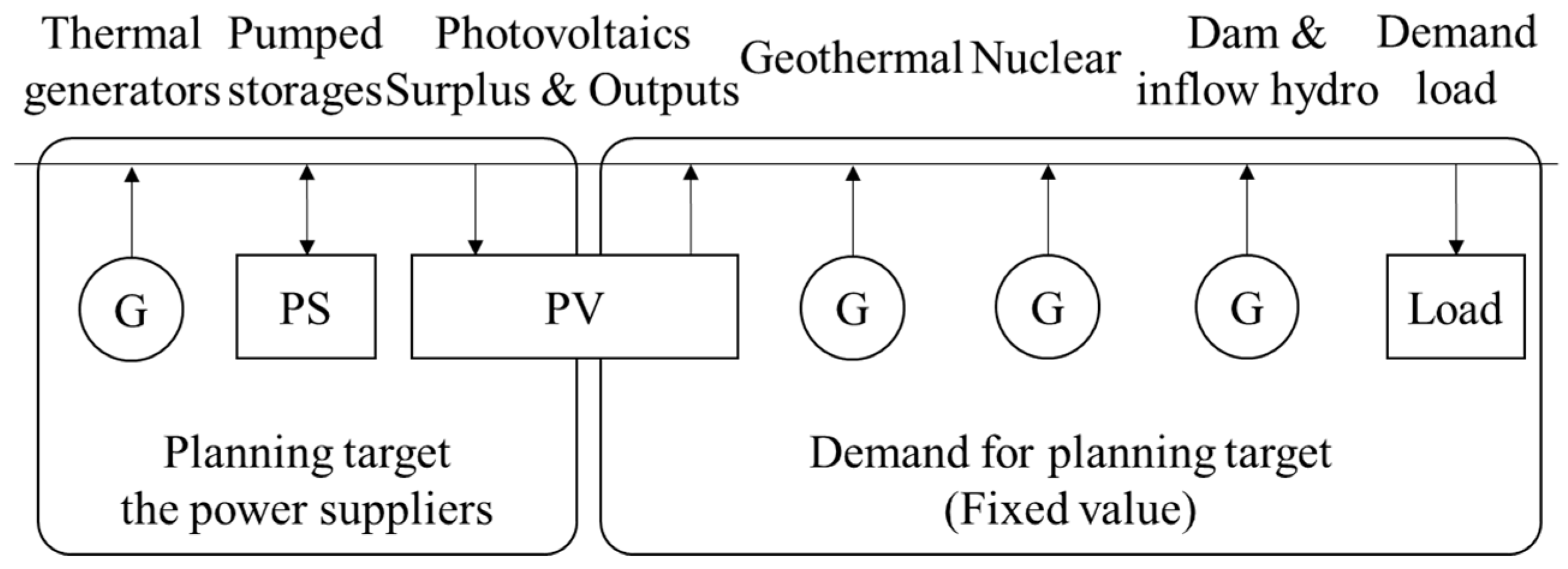
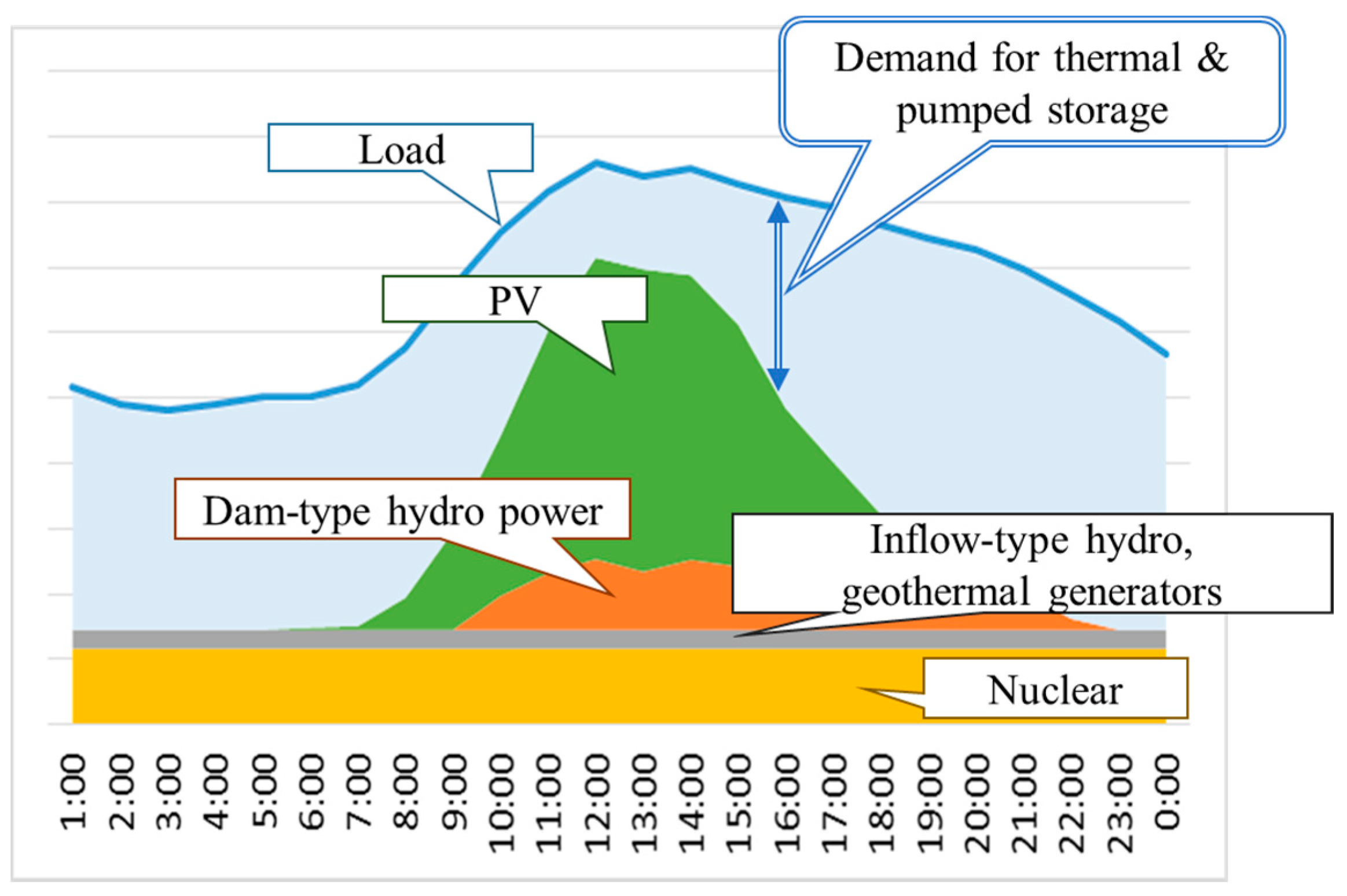
2.1. Overview

In order to study generators operation during the large-scale introduction of RESes, a unit commitment (start/stop plan) for the generators is formulated. As shown in Figure 1, the generators which are evaluated by this study are thermal power generators, pumped storages, and PV output control. On the other hand, nuclear, dam and inflow hydro, and geothermal power generators are considered as the base-load supplier, therefore, their output is basically fixed, except dam generation which is allotted to times of day when the load is large. The demand load is assumed to be mainly covered by these base-load supplier, with the remaining load is shared by thermal power generators and pumped storages. In addition, Figure 2 shows the power demand curve used in this study. The demanded power from thermal power generators and pumped storages are shown as a blue-colored area.

This study proposes a week-long operation plan model for formulating a unit commitment scheduling (start/stop plan) for thermal power generators and pumped storages in a certain area, especially in Japan, given the PV output and demand load presumed above. A week-based operation plans, 7 days including both weekdays and weekend to incorporate pumped storages, throughout a year (52 times) is modeled.

2.2. Modeling and System Conditions

2.2.1. Objective Function

Equation (1) is the objective function, F, which uses time increments of 1 week and formulates a plan covering 1 year, or 52 weeks. The equation minimizes fuel expenses and startup costs for thermal power generators. Furthermore, for simplicity’s sake, stop costs are not taken into consideration. Also, startup costs are fixed regardless of stop time:

$$Min.F={\displaystyle \sum _1^{52}\left[{\displaystyle \sum _t^{168}{\displaystyle \sum _i^M\{U_{it}{f}_i(P_{it})+C_i(U_{i,t-1},U_{it})\}}}\right]}$$

(1)

where, U, C, and M are state variable of unit commitment or start/stop condition (0 = stop, 1 = start), start-up cost, and number of generators, respectively. In addition, f_i(P_it) is generator fuel cost function of ith generator, which can be approximated as follows:

$$f_i(P_{it})=\text{}{a}_i{P}_{it}^2+b_i{P}_{it}+c_i$$

(2)

where, P_it is generator output of ith generator and at time t. Furthermore, a_i, b_i, and c_i are coefficients of fuel cost function for each corresponding order.

Furthermore, in this study, there are three main different system conditions (constraints) which are assumed: operating conditions of power system, mechanical constraints of generator, and operating limitations of pumped storage.

2.2.2. Operating Conditions of Power System

The operating conditions of power system are shown in Equations (3)–(6). Equation (3) expresses the supply and demand balance constraints, reconciling thermal power generators and pumped storages net output, PV output, and the amount of PV output suppression with the load:

$$P_{demand,t}=\sum _i{U}_{it}{P}_{it}+P_{output,t}^{Pump}-P_{pumpup,t}^{Pump}+P{V}_{output,t}-P{V}_{bound,t}$$

(3)

where, P_demand,t, PV_output,t, and PV_bound,t are demand load, PV output, and PV output suppression at corresponding time t, respectively. In addition, $P_{output,t}^{Pump}$ and $P_{pumpup,t}^{Pump}$ are output power during power generation and required power for pumping up at time t, correspondingly.

Equation (4) is a conditional expression that guarantees coordination to ensure the continuation of stable system operations if a prediction error regarding PV output occurs at a given point in time during the study. However, if PV output is redundant, it will be presumed to be suppressed, so the coordination of power output taking into account PV output suppression is guaranteed via thermal power generators at α% (coordination coefficient to respond to prediction errors of PV output) or higher:

$$\{\begin{array}{l}\alpha \cdot \left(P{V}_{output,t}-P{V}_{bound,t}\right)\le {\displaystyle \sum _i{U}_{it}\left(P_{\max ,i}^G-P_{it}\right)}\\ \text{}\alpha \cdot \left(P{V}_{output,t}-P{V}_{bound,t}\right)\le {\displaystyle \sum _i{U}_{it}\left(P_{it}-P_{\min ,i}^G\right)}\end{array}$$

(4)

where, $P_{\max ,i}^G$ and $P_{\min ,i}^G$ are maximum and minimum output considering the governor-free capacity of the ith generator, respectively.

Like Equation (4), Equation (5) guarantees coordination via thermal output generators at a load of β% (coordination coefficient to respond to prediction errors of demand load) or higher in order to ensure the continuation of stable system operations even if a prediction error regarding the load occurs at a given point in time during the study:

$$\{\begin{array}{l}\beta \cdot P_{demand,t}\le {\displaystyle \sum _i{U}_{it}\left(P_{\max ,i}^G-P_{it}\right)}\\ \beta \cdot P_{demand,t}\le {\displaystyle \sum _i{U}_{it}\left(P_{it}-P_{\min ,i}^G\right)}\end{array}$$

(5)

LFC constraint is expressed in Equation (6) [15]. As shown in Figure 3, it is a limiting equation that compares the geometric means of the load short-time fluctuation of x% (coefficient for designated LFC amount to respond to short-term fluctuations in demand for power at given time of day) and the PV output short-term fluctuation of y% (coefficient for designated LFC amount to respond to short-term fluctuations in PV output at given time of day), taking into account PV output suppression, and guarantees a number of active generators so that the rated output of active thermal power generators is z% (coefficient for generator rated output to respond to short-term fluctuations during a given time of day) or above:

$$\sqrt{{\left(P_{demand,t}\times x\right)}^2+{\left\{\left(P{V}_{output,t}-P{V}_{bound,t}\right)\times y\right\}}^2}\le {\displaystyle \sum \left|U_{it}\left(P_{\max ,i}*z\right)\right|}$$

(6)

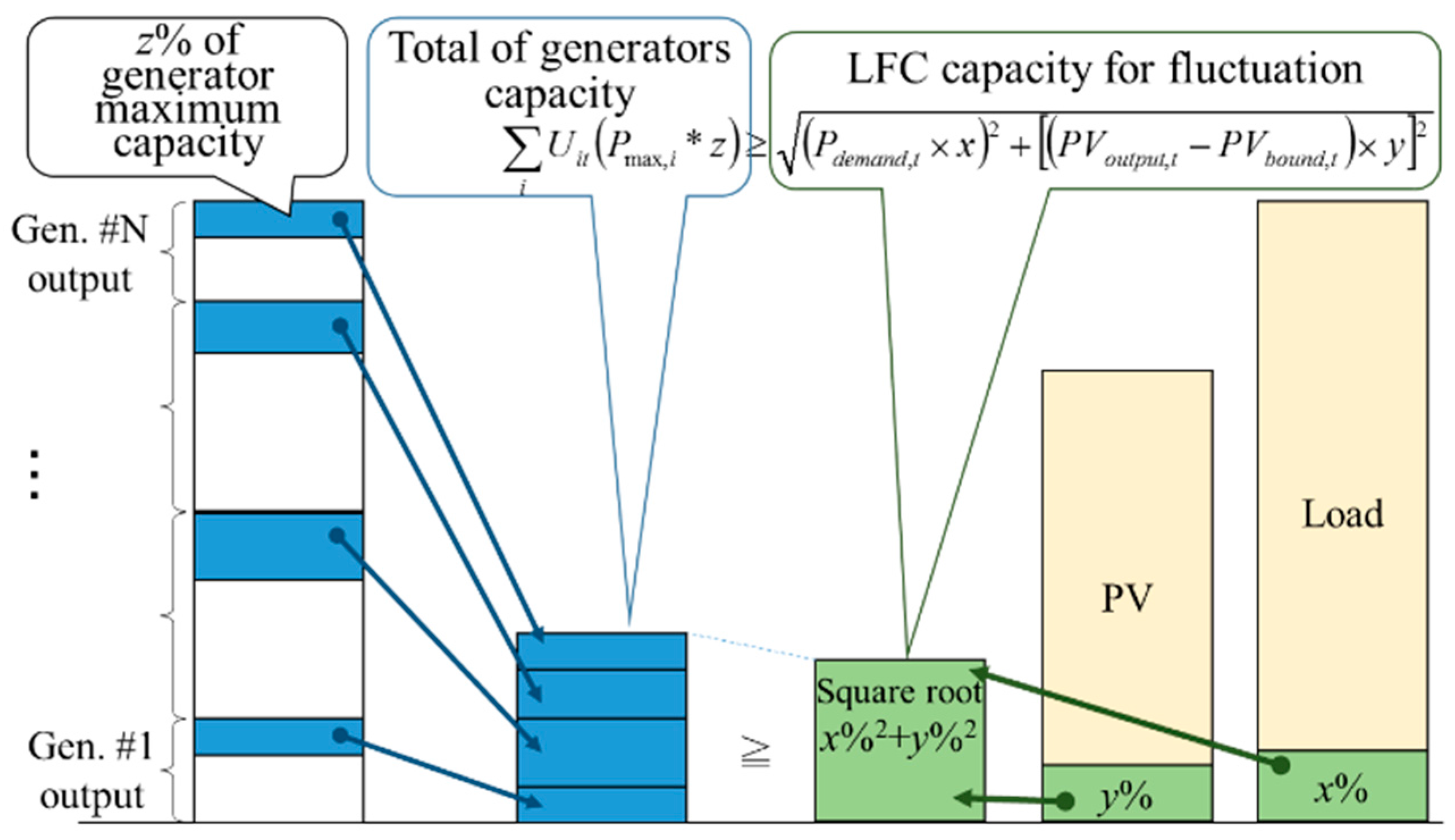
2.2.3. Mechanical Constraint of Generator

The mechanical limitations of thermal power generators are expressed in Equations (7)–(9). Equation (7) represents the ramp rate constraints that suppress the rate of change of output of each generator, which is a limiting condition spanning multiple times of day:

$$\left|P_{it}-P_{i,t-1}\right|\le \gamma$$

(7)

where, γ is limiting coefficient of changes in output.

Furthermore, Equation (8) represents the upper and lower limit constraints for the output of each generator. Also, in order to maintain the governor-free capacity, limitations that include governor-free capacity within the upper and lower limits of the mechanical limitations are established, as follows:

$$U_{it}{P}_{\min ,i}^G\le P_{it}\le U_{it}{P}_{\max ,i}^G$$

(8)

Generators must continue operations for a given period of time or longer once activated for a variety of reasons. Similarly, once stopped, generators should remain stopped. Equation (9) expresses the minimum starting-up or stopping time constraints for each generator that represent these limitations.

$$U_{it}\{\begin{array}{l}1:if0\le X_{it}\le MU{T}_i\\ 0:if0>X_{it}>-MD{T}_i\end{array}$$

(9)

where, X_it is defined as continuous time of ith generator for being activated or stopped. In addition MUT_i and MDT_i are minimum up time and minimum down time of ith generator, respectively:

$$X_{it}\{\begin{array}{l}{X}_{it}=X_{i,t-1}+1:X_{i,t-1}\ge 0,U_{it}=1\\ X_{it}=1:X_{i,t-1}<0,U_{it}=1\\ X_{it}=X_{i,t-1}-1:X_{i,t-1}<0,U_{it}=0\\ X_{it}=-1:X_{i,t-1}\ge 0,U_{it}=0\end{array}$$

(10)

2.2.4. Operating Limitations of Pumped Storage

The operating limitations of pumped storage plants can be approximated as Equations (11) and (12). Equation (11) expresses the upper and lower limits on pumped storage plant output. These are divided into plant generation conditions and pump power conditions and expressed:

$$\begin{array}{l}{P}_{gen}^{Pump}\le P_{output,t}^{Pump}\le 0\\ 0\le P_{pumpup,t}^{Pump}\le P_{up}^{Pump}\end{array}$$

(11)

where, $P_{gen}^{Pump}$ and $P_{up}^{Pump}$ are maximum output power during power generation and maximum power required for pumping-up, respectively.

In addition, Equation (12) expresses the limiting conditions regarding the storage capacity of the pumped storage plant:

$$0\le \eta {\displaystyle \sum _t^n\left(P_{pumpup,t}^{Pump}\right)}-\frac{1}{\eta }{\displaystyle \sum _t^n\left(P_{output,t}^{Pump}\right)}\le P_{capcity}^{Pump};n=1,2,\dots \dots ,168$$

(12)

where, η is operational efficiency of pumped storage.

3. Unit Commitment Schedule for Thermal Power Generators and Pumped Storages

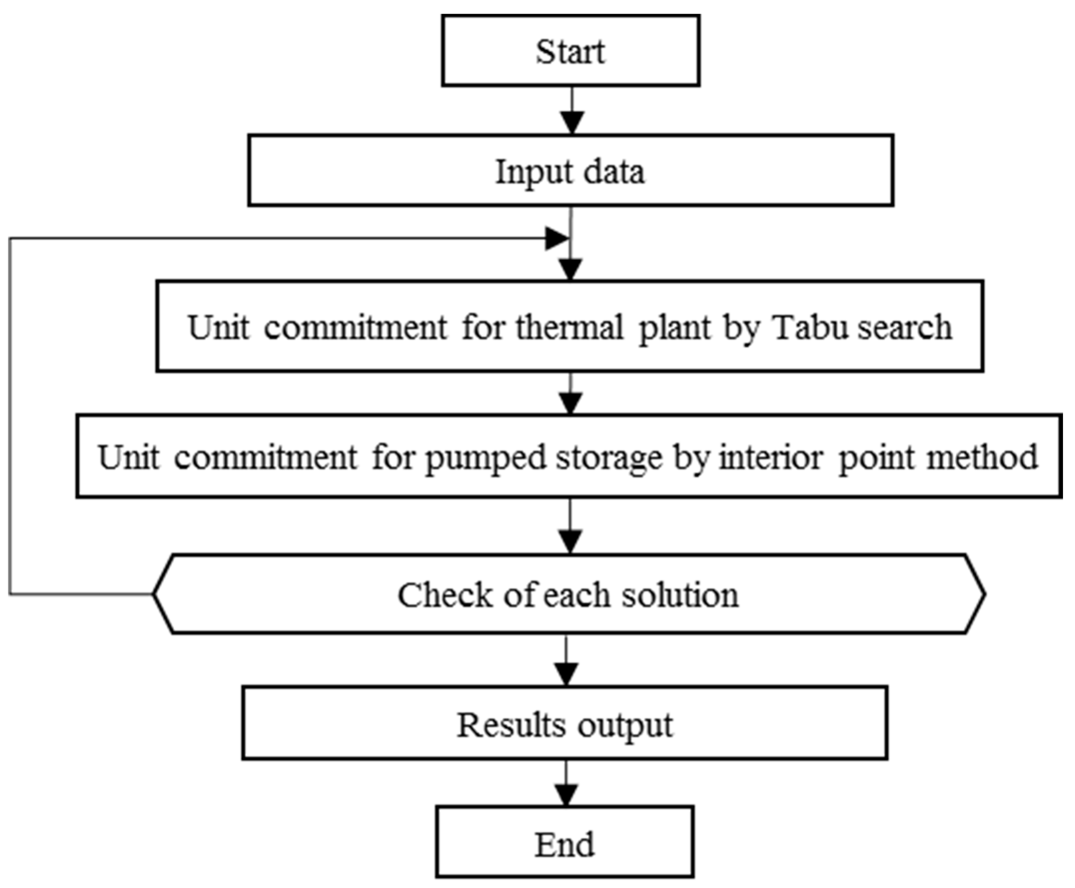
3.1. Overview of Proposed Method

The issues defined in equations in Section 2.2 determine the optimum application of thermal power generator and pumped storages. However, in order to solve for all the decision variables simultaneously, the calculation time must be extended. Therefore, the plans for the operation of thermal power generators and pumped storages are separated; the operation status of each is held constant, and as each side resolves the problems of the other, the solutions for the separate issues are converged. The calculation process is flowcharted in Figure 4.

The generator start/stop status U_it is a decision variable set as 0 or 1, and the generator output Pit is a variable subordinate to U_it. Pit applies the lambda-iteration method and is determined by the economic load dispatch (ELD).

On the other hand, the operation of the pumped storages is determined by the interior point method and the operation status of the thermal power generators determined by the Tabu search (U_it, P_it) is fixed. The use plans for the thermal power generators and the pumped storages resolve each other, and when the solutions are converged, the calculations are concluded.

3.2. Operating Plan for the Thermal Power Generators

With the issues that determine the use status of thermal power generators, the use status of the pumped storages is held constant, and a Tabu search is employed. From Equation (1), the objective function for the formulated problem, the U_it limitation only connects the time period t − 1 and the time period t; otherwise, the generator i and the time period t are completely separated. On the other hand, Equations (3)–(9), the limiting-condition equations, connect the ith generator with the other generators, and separating them is difficult. Therefore, the limiting conditions are relaxed to the objective function via a penalty coefficient method, and by applying a Tabu search, a suboptimal solution that fulfills the limiting conditions can be obtained.

As U_it is altered in a Tabu search, the limiting conditions are not necessary fulfilled by the neighborhood solutions. Therefore, in order to lead U_it in a direction that fulfills the limiting conditions, the penalty coefficients are multiplied to the degree to which the limiting conditions are violated and included in the objective function to relax it. The relaxed objective function used in the Tabu search is represented in Equation (13) below:

$$\begin{array}{cc}\hfill Min.F_{new}=F& +Penalty1\times h_1+Penalty2\times h_2\hfill \\ & +Penalty3\times h_3+Penalty4\times h_4\hfill \\ & +Penalty5\times h_5+Penalty6\times h_6\hfill \end{array}$$

(13)

where, Penalty 1 to Penalty 6 are penalty coefficients to represent the degree to which each limiting condition is violated

In addition, Equations (14)–(16) are meant to organize and represent Equations (17)–(20):

$$A=\alpha \cdot \left(P{V}_{output,t}-P{V}_{bound,t}\right)$$

(14)

$$B={\displaystyle \sum _i{U}_{it}\left(P_{\max ,i}-P_{it}\right)}$$

(15)

$$C={\displaystyle \sum _i{U}_{it}\left(P_{it}-P_{\min ,i}\right)}$$

(16)

$$h_1={\displaystyle \sum CP{V}_t^{\max }}=\{\begin{array}{ll}CP{V}_t^{\max }=0& :A\le B\\ CP{V}_t^{\max }=A-B& :A>B\end{array}$$

(17)

$$h_2={\displaystyle \sum CP{V}_t^{\min }}=\{\begin{array}{ll}CP{V}_t^{\min }=0& :A\le C\\ CP{V}_t^{\min }=A-C& :A>C\end{array}$$

(18)

$$h_3={\displaystyle \sum CDe{m}_t^{\max }}=\{\begin{array}{ll}CDe{m}_t^{\max }=0& :\beta \cdot P_{demand,t}\le B\\ CDe{m}_t^{\max }=\beta \cdot P_{demand,t}-B& :\beta \cdot P_{demand,t}>B\end{array}$$

(19)

$$h_4={\displaystyle \sum CDe{m}_t^{\min }}=\{\begin{array}{ll}CDe{m}_t^{\min }=0& :\beta \cdot P_{demand,t}\le C\\ CDe{m}_t^{\min }=\beta \cdot P_{demand,t}-C& :\beta \cdot P_{demand,t}>C\end{array}$$

(20)

$$h_5={\displaystyle \sum CLF{C}_t}=\{\begin{array}{c}CLF{C}_t=0\left(\sqrt{{\left(P_{demand,t}\times x\right)}^2+{\left(P{V}_{output,t}\times y\right)}^2}\le {\displaystyle \sum \left|U_{it}\left(P_{\max ,i}*z\right)\right|}\right)\hfill \\ CLF{C}_t=\sqrt{{\left(P_{demand,t}\times x\right)}^2+{\left(P{V}_{output,t}\times y\right)}^2}-{\displaystyle \sum \left|U_{it}\left(P_{\max ,i}*z\right)\right|}\hfill \\ \left(\sqrt{{\left(P_{demand,t}\times x\right)}^2+{\left(P{V}_{output,t}\times y\right)}^2}>{\displaystyle \sum \left|U_{it}\left(P_{\max ,i}*z\right)\right|}\right)\hfill \end{array}$$

(21)

$$h_6={\displaystyle \sum Z_i}=\{\begin{array}{ll}{Z}_i=X_{it}-MUT& \left(X_{it}-MUT>0,X_{it}>0\right)\\ Z_i=-X_{it}-MDT& \left(-X_{it}-MUT>0,X_{it}<0\right)\end{array}$$

(22)

Using Equation (13), the relaxed objective function, the issue of the optimum use plan for the thermal power generators is formulated. The solution in the Tabu search is the variable (0 or 1) for the start/stop condition for the thermal power generator in each time period. The neighborhood solution approaches 1, and the terms of the current solution of U_it are changed in one spot only. The Tabu length of the parameter in the Tabu search is set at the number of generators and repeated at specified number of times, whereby the suboptimal solution is found.

3.3. Operating Plan for Pumped Storage

The objective function related to the formulation of a plan for use of pumped storages is not directly included in the original problem formulated in Section 2.2. Therefore, the objective function used for the pumped storages operation plan needs to be newly defined. By fixing the status of the thermal power generators, it is possible to calculate the average unit fuel cost for each time period. By generating power using pumped storages at time periods when the average unit fuel cost for thermal power generators is high, it is possible to decrease their operational costs. In addition, the work consumed for pumping up the water by pumped storages can be provided in case of low fuel cost for thermal power generators and also during time periods when PV output is suppressed, therefore, the suppressed portion can be proactively used as power. In the latter case, it is presumed as freely available power. Furthermore, if there are often multiple pumped storages in a region, they are presumed to be aggregated into one. Equation (23) represents the objective function for the optimization problem of the operation plan for the pumped storages. The limiting conditions are represented in Equations (10)–(12):

$$Min.F={\displaystyle \sum _T^{52}\left[{\displaystyle \sum _t^{168}aveC(P_{output,t}^{pump})}\right]}$$

(23)

where, aveC is the average unit fuel cost by time period.

The interior point method is applied to the objective function of Equation (23) and the limiting conditions expressed in Equations (10)–(12) to obtain an optimal solution. Interior point method is considered as the most reliable method to solve the optimal power flow [25].

3.4. Acceleration of Calculations

To accelerate the calculations used in this study, two steps are performed: (1) simplification of complex limiting conditions, and (2) reducing the number of neighborhood solutions in Tabu search.

3.4.1. Simplification of Complex Limiting Conditions

By changing Equation (6), the LFC limitation formulated, the number of variables included in the limiting conditions can be reduced. When the first term on the right side of Equation (3) is transposed to the left side and substituted into Equation (5), and both sides are raised to the power of 2, the result is as depicted in Equation (24):

$${\left(P_{demand,t}\times x\right)}^2+\left[\left(P_{demand,t}-{\displaystyle \sum _i{U}_{it}{P}_{it}}\right)\times y\right]\le {\left[{\displaystyle \sum _i{U}_{it}\left(P_{\max ,i}\times z\right)}\right]}^2$$

(24)

In Equation (24), the variable representing the suppression of PV output can be omitted from the limiting conditions, thus simplifying them. The PV output suppression variable can also be omitted from Equation (3) in the same manner. Therefore, the PV output suppression variable from the thermal power generator operation plan can be contained to Equation (3).

3.4.2. Reducing the Number of Neighborhood Solutions in Tabu Search

The Tabu search applied to the thermal power generator optimization presents a high calculation burden for the objective function of the neighborhood solution. This study focuses on the thermal power generator operating terms constrained by the operating conditions and reduces the number of neighborhood solutions.

In Equation (5), the limiting equation for the prediction error for the load, the left side is a fixed value for each time period t, so it determines the minimum number of activated generators for the generator activation state U_it. Therefore, if the number of activated generators falls below the necessary number in the limiting conditions, it is assumed that the generators will not be switched to a stop state, and neighborhood solutions that switch activated generators to a stopped status will not be created. Through this operation, the number of neighborhood solutions calculated is reduced.

Similarly, Equation (4) used as a limiting equation for prediction errors for PV output, and the number of neighborhood solutions is reduced so that the number of active generators does not fall below the minimum.

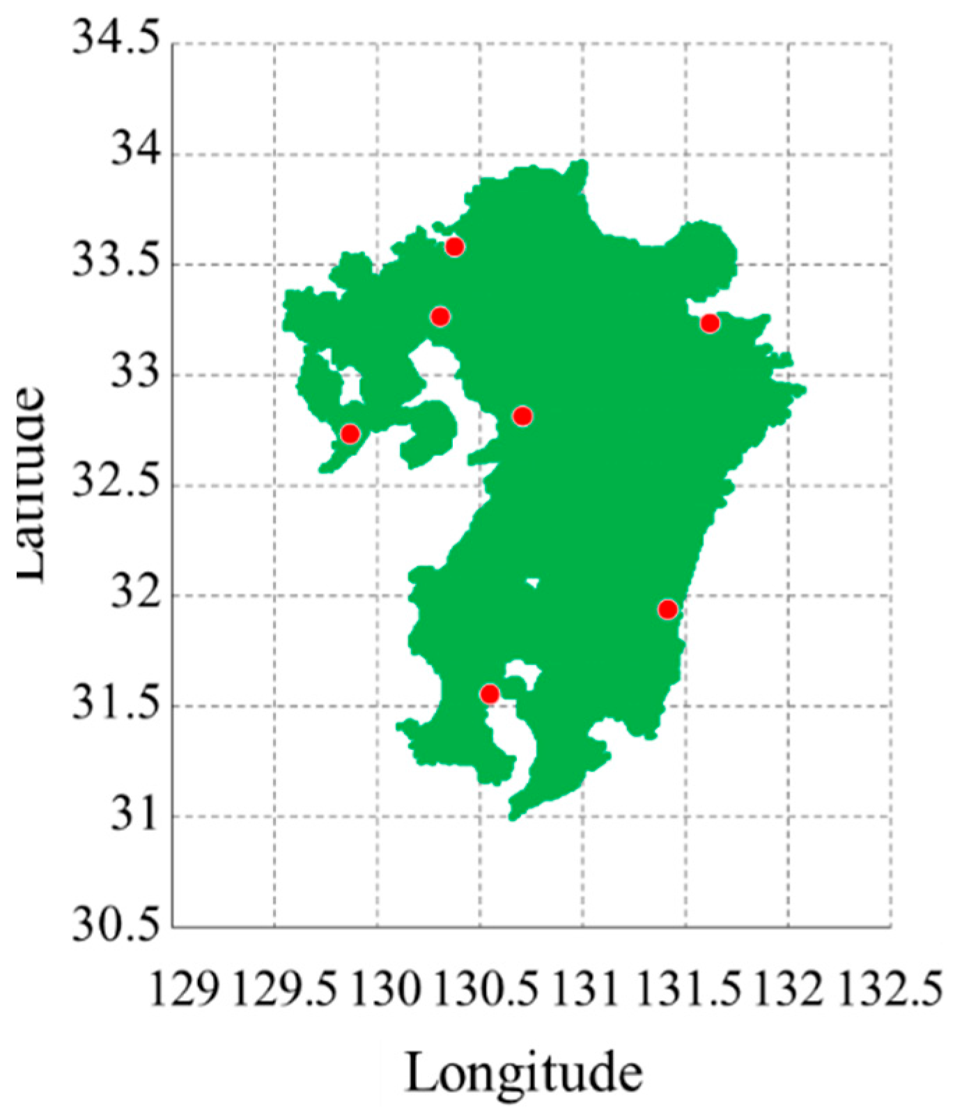
4. Area Selection and Example of Numerical Calculation

Numerical calculation is carried out using the methods proposed so far until Section 3 and the validity of the method is examined. The system capacity, transmission capacity, authorized PV installation amount, PV introduction situation and connectable amount of each region in Japan refers to [26] and are shown in Figure 5.

In the Kyushu region, the PV introduction is about 4 GW at the end of 2014, which is about 20% of the system capacity of about 20 GW. The authorized PV installation amount is 18 GW, which is almost the same as the system capacity. Furthermore, since the transmission capacity with other power generators is also small, it is assumed that the system operation becomes difficult in the near future compared to other areas, and the suppression of PV output is required. Therefore, in this study, the numerical calculation is applied for the Kyushu region.

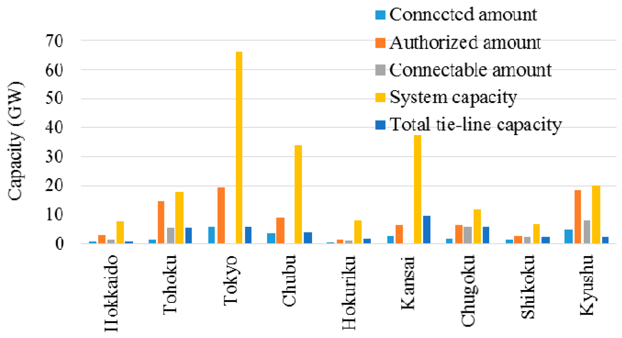
4.1. Conditions of Numerical Calculation

The monthly total output of inflow- and dam-types of hydro power, pumped storages, geothermal power and nuclear power in the Kyushu region and the electric power demand per hour are based on the actual data published in 2014 [26].

The hourly PV output is estimated from solar radiation data of the Japan Meteorological Agency using the method used in [27]. 1-hour data of seven total solar radiation amounts for each prefecture in the Kyushu region are used, as shown in Figure 6. The configuration of the PV system is assumed to be south oriented with the inclination angle of 30° and PV output is assumed to be uniformly introduced.

The type and number of generators existing in the Kyushu region have been published in [28], but it does not include the generator characteristics such as fuel cost function and start-up cost. In the numerical calculation, the average fuel cost of various generators [29,30] and the modified Institute Of Energy Economics Japan (IEEJ) power system standard model [31] are used. The characteristic values of each generator are shown in

Table 1. Specifications of generators involved in the analysis.

Generator Class	ai	bi	ci	Start-Up Cost [M-JPY]	MUT [Time]	MDT [Time]	PGFi,min [MW]	PGFi,max [MW]	Number
Coal 1000 MW	0.00005	1.1	120	1200	10	8	550	950	4
Coal 700 MW	0.0004	3.25	450	3000	5	8	110	665	3
Coal 200 MW	0.0005	5.0	100	2000	5	8	80	340	1
Oil 500 MW	0.00016	17.0	700	10,000	3	4	105	475	7
Oil 250 MW	0.0031	16.0	900	8000	3	4	105	360	2
LNG 700 MW	0.0009	8.6	400	6000	2	3	125	570	3
CC 100 MW	0.004	4.0	420	1000	1	1	40	110	6
CC 250 MW	0.006	5.0	400	2000	1	1	60	210	4
CC 250 MW	0.006	5.0	400	2500	1	1	70	230	3
Pumped storage								2350	1
							Total	17,990	34

.

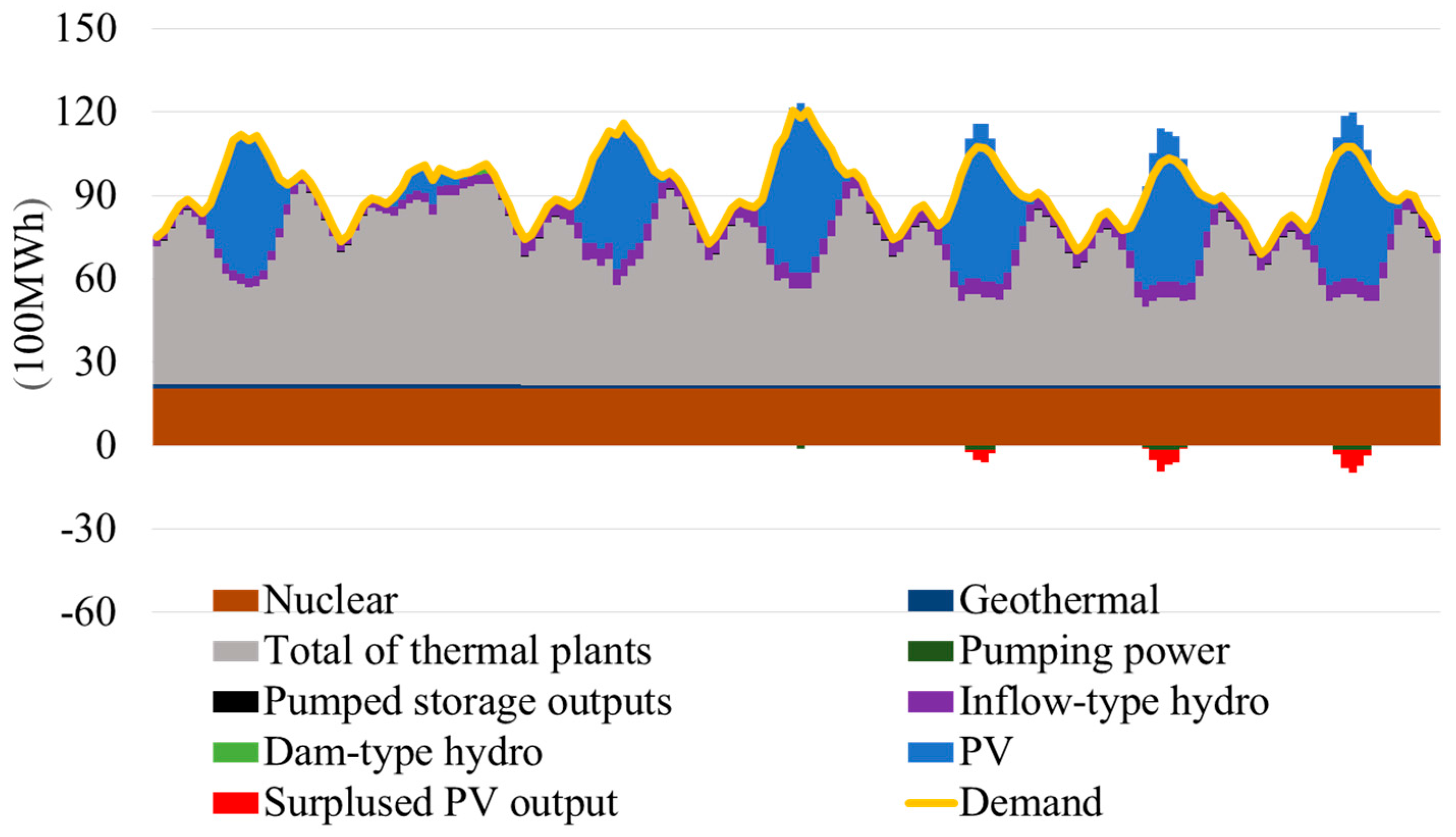
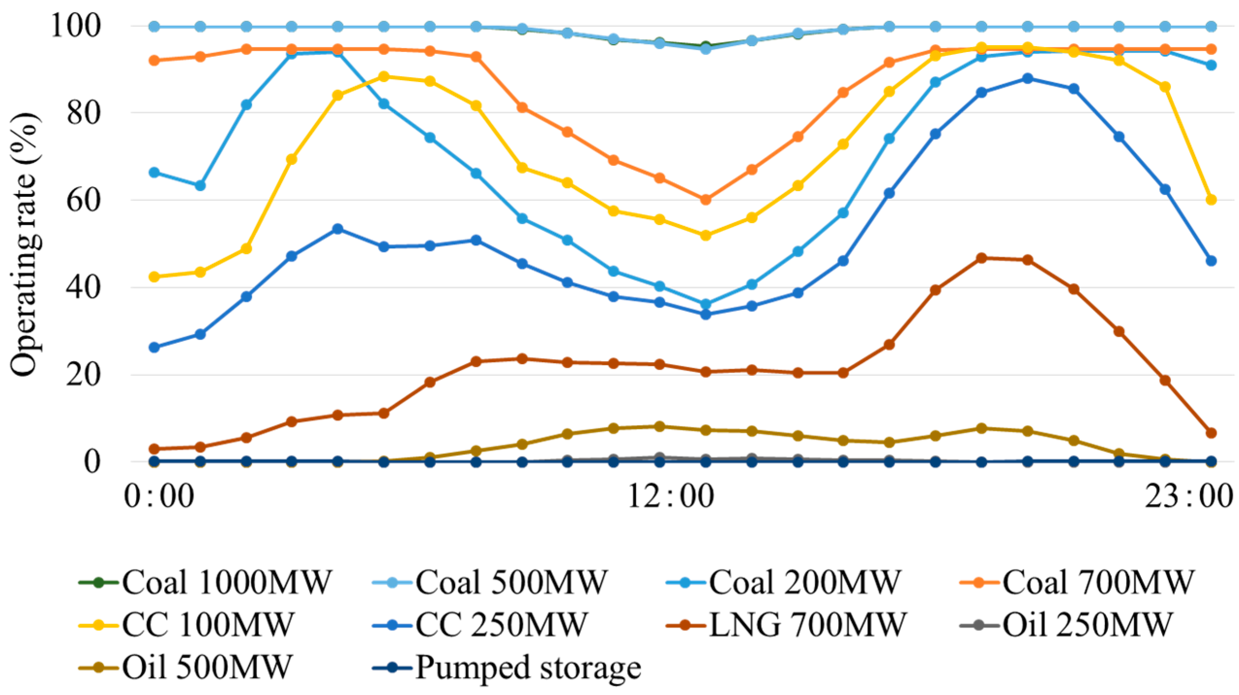
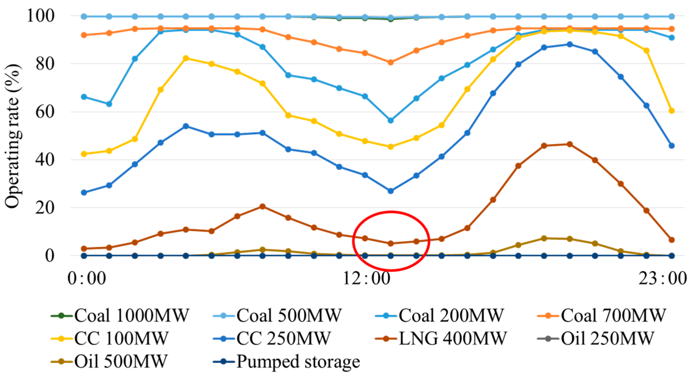
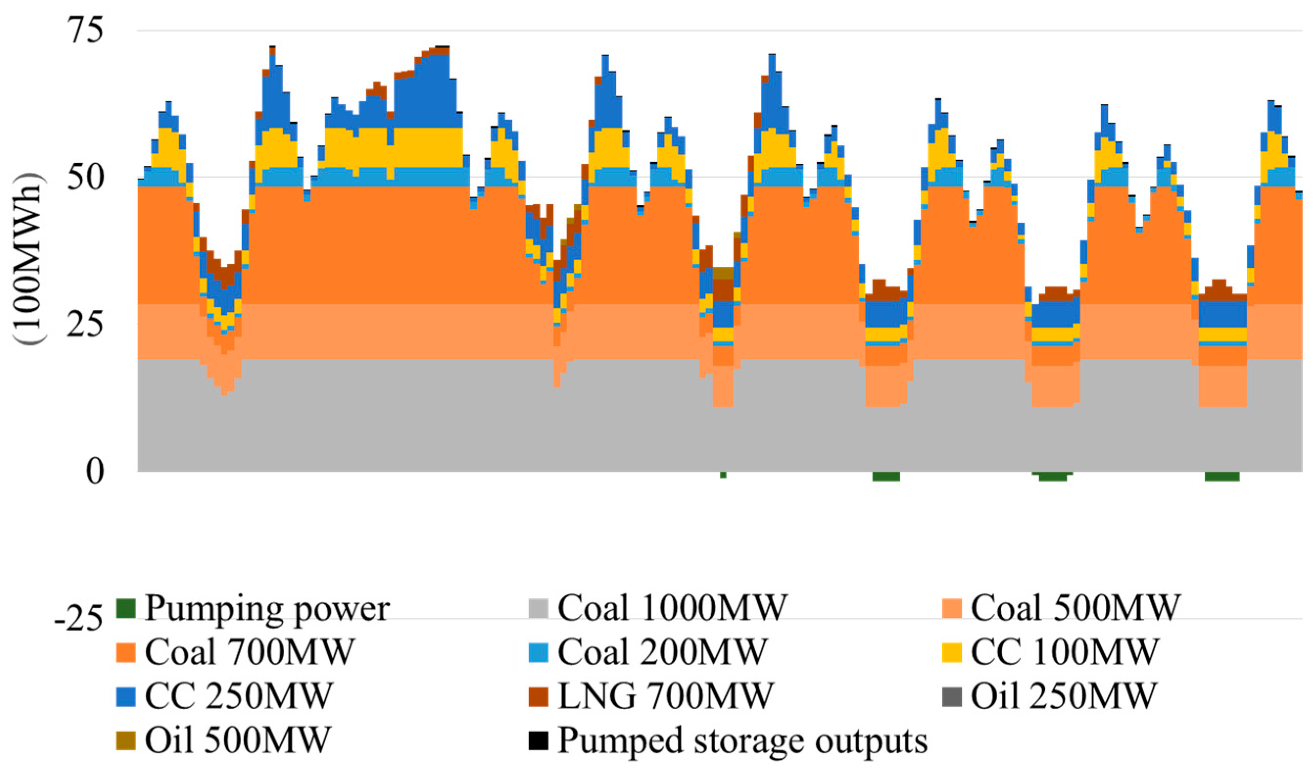
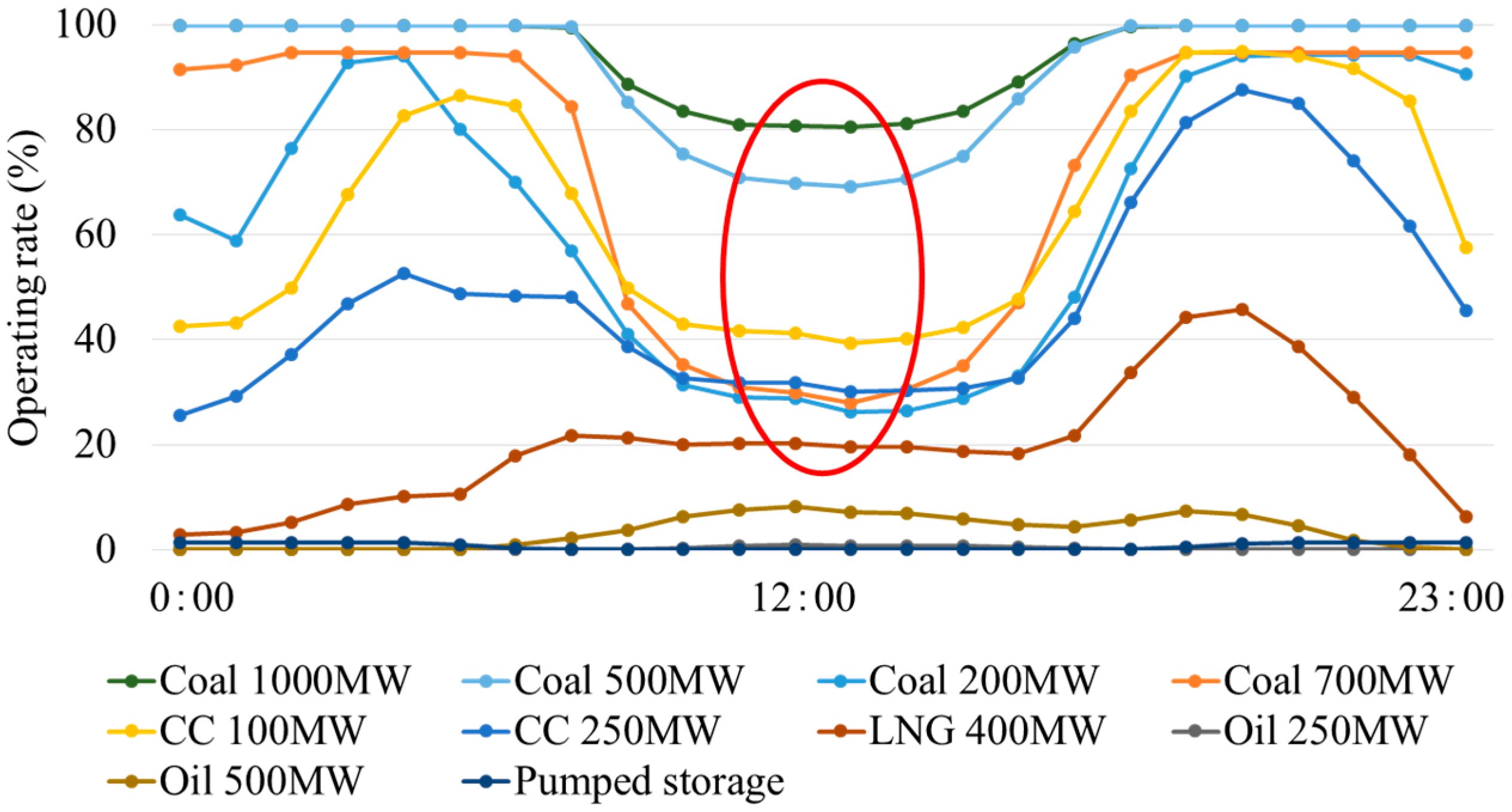
4.2. Numerical Results

Year-round numerical calculations are carried out under the conditions of calculation described in Section 4.1. However, the capacity of the nuclear power plant is set at 2.35 GW, and the operation rate is made constant with reference to 80% [32], which is the average operation rate of domestic pressurized water nuclear power plants before the Great East Japan Earthquake. Moreover, the PV introduction amount is assumed to be 8.17 GW as the connectable amount in Kyushu Electric Power [33].

Figure 7 and Figure 8 show the calculation results extracted for the golden week holidays (29 April to 5 May 2014) with low power demand and relatively high PV output in the intermediate period. In Figure 7 and Figure 8, the ordinate and abscissa indicate the amount of electric power and the time, respectively. Figure 7 shows the total generated electricity including PV and the like. Figure 8 shows the amount of power generated by various thermal power generators and pumped storage, and breakdown of the total firepower is shown in the grey area in Figure 7.

The obtained numerical calculation results satisfy all the constraint conditions, and it is considered that reasonable results are obtained because the thermal power generators are started in the order of the lowest fuel cost. In the calculation results, in that week, the PV output gives a surplus of 2% in terms of electricity ratio. Part of the surplus electricity is used as a pumping power to reduce its extent. However, in the case of this calculation, since the operation plan is drawn up with the upper limit value of the generated electricity amount of the pumped storage according to the actual result, the reduction of the electric power surplus is not sufficient.

Calculation of the numerical values is performed under the conditions that the PV capacity is set at 4,080,000 kW and the nuclear power plant is stopped. This is almost the same with the actual operation condition in 2014 [32]. As the results of calculation, the calculated electricity amount for thermal power generators and others (including pumped storages) are 50.2 and 27.9 TWh, respectively. On the other hand, the actual amount of electricity by thermal power generators and others were 50.4 and 27.8 TWh, respectively. Therefore, the accuracy of the performed numerical calculation is very high (99.6%) for both thermal power generators and other generators. In addition, regarding the operating rate of thermal power generators, the numerical calculation also shows very high similarity with the actual value, which are 63.21% and 63.43%, respectively.

It is understood that the actual value in 2014 and the value obtained by numerical calculation are substantially the same. As a result, it can be considered that reasonable calculation results are obtained by the constructed model and simulator. Furthermore, the execution time on an Intel core i7 3.4 GHz memory 8 GB PC is about 8 h.

5. Year-Round Evaluation by the Proposed Method

Using the method proposed up to the Section 4, now year-round evaluations of operating rates and operational costs of thermal power generators are performed.

5.1. Explanation of Parameters

To perform year-round evaluation using the proposed method, the installed capacity of the nuclear power plant, the introduction amount of PV and the coefficient of LFC constraint for PV fluctuation are used as parameters to compare and study the annual operational costs, etc.

The PV introduction amount of 8.17 GW is considered as 100%. The total capacity of the nuclear power plants that could operate in 2016 is 4.7 GW, which is assumed to be 100% of the nuclear capacity. Supposing that the assumed lifetime is 40 years after construction, the reactors will be decommissioned in 2030, the remaining capacity is 2.35 GW and the nuclear capacity is 50%. This is considered as the base case. The annual operating rate is assumed to be 80% and the LFC coefficient y for PV in LFC constraint is set to 5% [7].

By changing these three parameters as shown in

Table 2. Parameters for analysis including nuclear, PV, and LFC.

Generator	Share			Number of Patterns
Nuclear	0%, 25%	50%	75%, 100%	5
PV	50%, 75%	100%	125%, 150%, 175%, 200%	7
LFC	0%, 2.5%	5%	7.5%, 10%	5

, the annual operating rate and the annual operational cost are examined. In Table 2, the shaded central parameters constitute the base case.

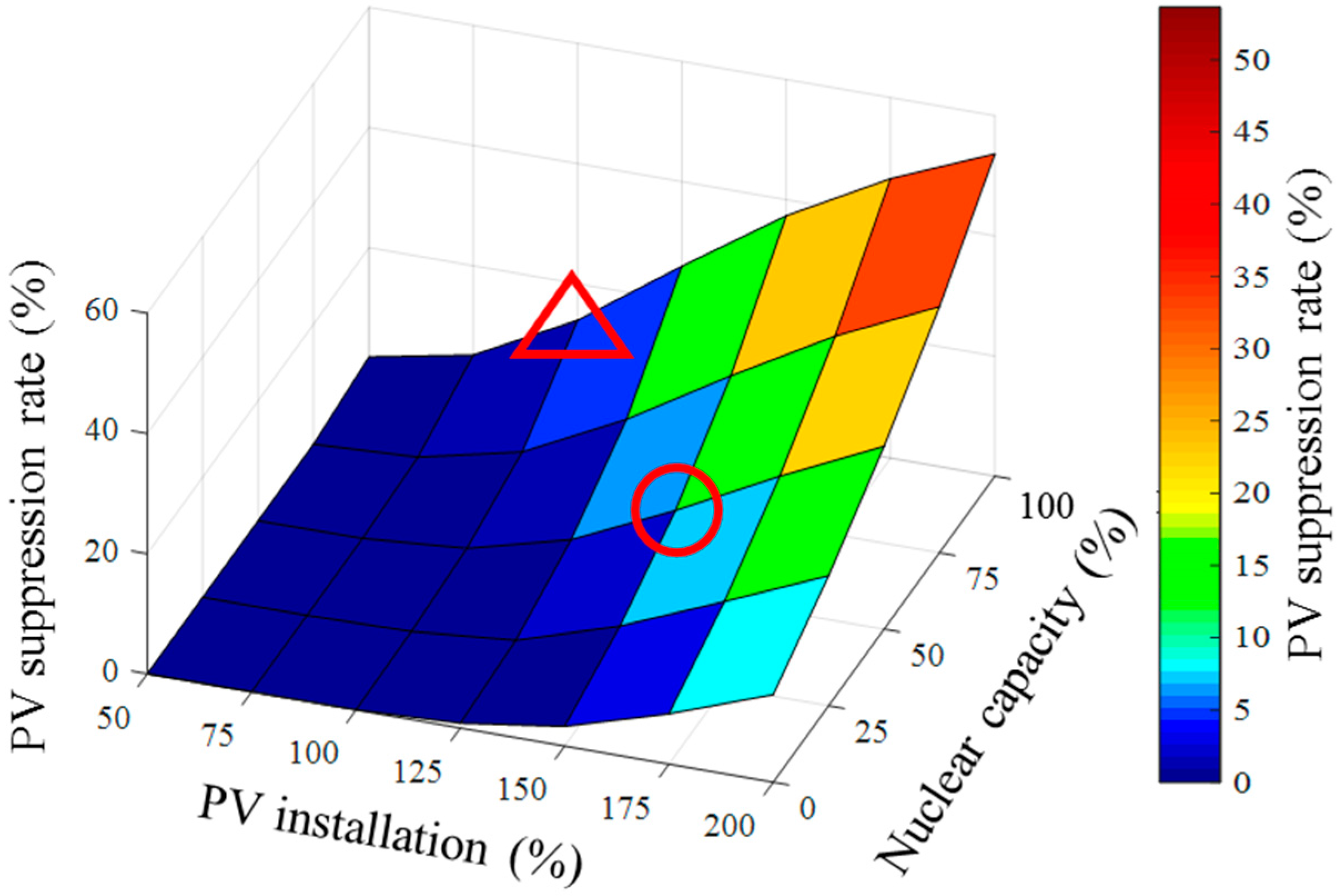
5.2. Impact of Nuclear Power Capacity and PV Introduction Amount onto the PV Surplus Rate

The PV surplus ratio is examined using the nuclear power capacity and the PV introduction amount as parameters. The PV surplus rate is expressed by the Equation (25):

$$PV\mathrm{surplus}\mathrm{rate}[\%]=\frac{\mathrm{Total}PV\mathrm{surplus}\mathrm{of}\mathrm{the}\mathrm{year}[\mathrm{TWh}]}{\mathrm{Total}PV\mathrm{output}\mathrm{of}\mathrm{the}\mathrm{year}[\mathrm{TWh}]}$$

(25)

Figure 9 summarizes the results of calculating a total of 35 cases using nuclear capacity and PV introduction amount as parameters. With the increase of PV introduction amount, the PV surplus rate increases. Furthermore, since the nuclear power plant is assumed to have a constant output, as the nuclear capacity increases, the adjustment allowance of the thermal power generators is jeopardized, and thereby the PV surplus rate also increases proportionately.

In the future, when increasing the PV introduction amount, in order to make effective use of the PV output, it is useful to review the rated output constant operation of the nuclear power plant. Furthermore, when both the nuclear capacity and PV introduction amount are 100%, a surplus PV output is generated. It is understood that the PV connectable amount (equivalent to 100%) assumed by the electric power company is based on the premise that almost the totality of the existing nuclear power plants are in operation. Assuming that a PV surplus rate of the same level as the power company’s assumption is allowed, if the nuclear power plant is decommissioned as specified and halved by 2030, the PV introduction upper limit will be increased by about 1.5 times (From “△” to “○” in Figure 9).

5.3. Effect of PV Introduction Amount

Figure 10 and Figure 11 show the results of numerical calculation of the Base case and when the PV introduction amount is increased to 200% as an extreme example, respectively. Since the PV output is higher in daytime, the circle in Figure 11 indicates that the operational cost of coal-fired power generator, which is inherently low in fuel cost and desired to operate at constant rated power, is decreasing. In order to utilize the PV output, the output of coal-fired power generator which is an inexpensive power generator is reduced, the average electricity generation price of the thermal power generator at 12 o’clock increases from 4.65 JPY/kWh to 5.49 JPY/kWh, and the average generation price rises by about 18%. The reason is that in an environment where PV is massively introduced, the thermal power generator is in the state of partial load operation and the power generation efficiency is lowered.

5.4. Impact of the Intensity of LFC Constraints

Based on the results in Section 5.3, the impact of the intensity of LFC constraints on the hourly load factor of the generator is examined. Figure 12 and Figure 13 show the calculation results when the LFC constraint y is 0% and 10% from the base case, respectively.

Comparing Figure 10 (base case) and Figure 12 (10% LFC constraint), the load factor (ocher line) of the oil-fired power plant that operates at 10% or less during the day in Figure 10 is nearly 0% as shown in the circle in Figure 12. On the other hand, when comparing the result of Figure 10 and Figure 13 (10% LFC constraint), the load factor of the oil-fired power plant at daytime marked with red in Figure 13 is high. The reason is that the number of generators to be secured for compensating the output fluctuation varies depending on the intensity of LFC constraint with respect to the short-time fluctuation of PV output. This indicates that it is necessary to operate a generator with high fuel cost if the LFC constraint is overestimated.

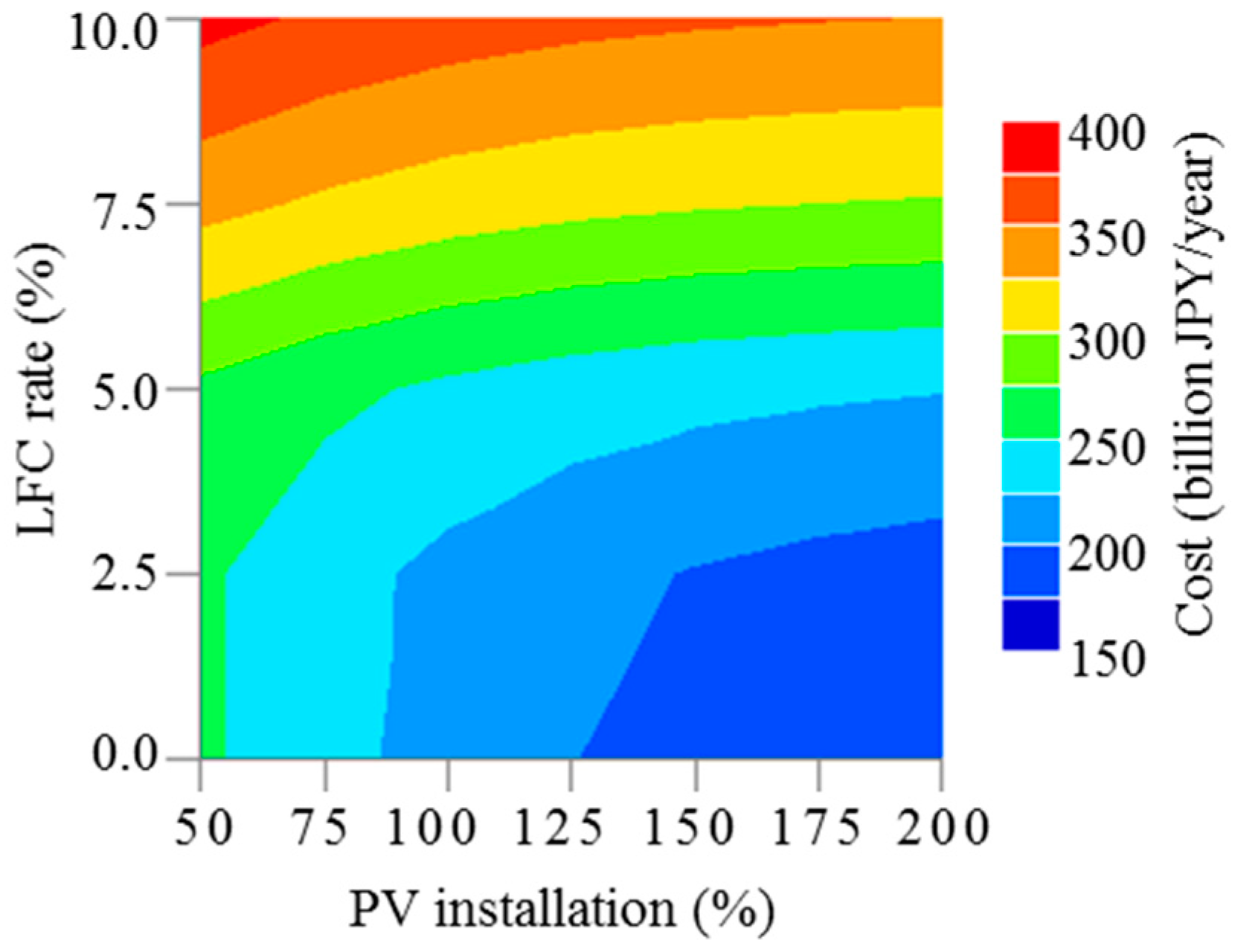
5.5. Impact of LFC Constraints on Operational Costs

The annual operational costs are examined using the PV introduction amount and the intensity of LFC constraints as parameters. The results of calculating 35 cases in total are summarized in Figure 14 and

Table 3. Calculation results for operational cost (billion JPY).

LFC y (%)	PV Introduction Rate (%)
	50	75	100	125	150	175	200
0.0	254	233	215	201	190	182	177
2.5	254	234	218	207	199	193	189
5.0	270	256	245	237	232	228	226
7.5	333	321	312	306	302	300	298
10.0	382	371	362	357	353	351	349

. Table 3 shows the operational cost based on the results of numerical calculations shown in Figure 14.

Regarding the generator parameters used for this numerical calculation, when the PV introduction rate is 50% (shaded portion in Table 3), by changing the LFC constraint y from 0% to 5%, the annual operational cost increases from about 254 billion JPY to about 270 billion JPY, meaning an increase of about 16 billion JPY and a proportion of about 6%. This can be considered as a resource for controlling 5% of the LFC constraint by a power generator other than the thermal power generator of the electric power company. Likewise, considering a PV introduction rate of 200%, the sum is about 49 billion JPY annually, about 22% of the annual operational cost. Taking into account the depreciation period, possibilities have been identified to create resources for covering costs of electricity storage facilities, demand response, etc.

6. Conclusions

A weekly unit commitment schedule (start/stop planning) for thermal power generator and pumped storages has been modeled and also calculated for 1 year (52 weeks, a year-round evaluation). To solve the generator start/stop planning problem, the proposed method solves both the operation planning problem for the thermal power generators and the output decision problem for the pumped storages.

The proposed method is also able to evaluate the changes in annual operational costs and changes in generator operating rate, depending on the PV introduction rate, the capacity of nuclear power plant facilities and LFC constraints. It is demonstrated that the proposed method can analyze a one-year evaluation within practical time. Numerically, the accuracy of the calculation using the proposed approach is about 99.5% for the evaluated Kyushu region. In addition, by assuming LFC constraints to cope with PV output fluctuations, the impact of the intensity of LFC constraints on the operational cost of the thermal power generator has been elucidated. The increment of the operational cost of the power supply with increasing PV introduction amount has been shown in concrete terms. By changing the LFC constraint of 0% to 5%, the annual operational costs in case of PV introduction rates of 50% and 200% increase from 254 to 270 billion JPY (6%), and from 177 to 226 billion JPY (22%), respectively.

If the adjustment power (LFC constraint) for the PV output fluctuation is overestimated on the side of the electric power system, the surplus of PV output increases. Therefore, even if PV introduction amount is increased further, the extent of contribution of thermal power generators to the reduction of fuel consumption is small.

Since the operation of the pumped storages is formulated based on the actual value in 2014, future tasks include the reduction of annual operating rate to as low as 0.7%. To consider the reduction of the PV output surplus, etc. by raising the operating rate, the operational costs and the PV surplus rate are the subject of studies using the pumped storage operation rate as a parameter.

In addition, the proposed approach can also be applied to other electric power markets. Especially, it will be effective for a markets with high share of wind and/or without any nuclear power plant. In addition, it also applicable for biomass power generator, although the priority between conventional thermal and biomass power generators may not be able to be determined only using cost analysis, but also other factors, such as CO₂ minimization, etc.

References

1. Zhang, J.; Hu, Z.; Zheng, Y.; Zhou, Y.; Wan, Z. Sectoral Electricity Consumption and Economic Growth: The Time Difference Case of China, 2006–2015. Energies 2017, 10, 249. [Google Scholar] [CrossRef]
2. Aziz, M. Integrated Supercritical Water Gasification and a Combined Cycle for Microalgal Utilization. Energy Convers. Manag. 2015, 91, 140–148. [Google Scholar] [CrossRef]
3. Ministry of Economy, Trade and Industry. Present Status and Promotion Measures for the Introduction of Renewable Energy in Japan. Available online: http://www.meti.go.jp/english/policy/energy_environment/renewable/ (accessed on 20 April 2016).
4. Komiyama, R.; Fujii, Y. Assessment of Post-Fukushima Renewable Energy Policy in Japan’s Nation-Wide Power Grid. Energy Policy 2017, 101, 594–611. [Google Scholar] [CrossRef]
5. Komiyama, R.; Fujii, Y. Assessment of Massive Integration of Photovoltaic System Considering Rechargeable Battery in Japan with High Time-Resolution Optimal Power Generation Mix Model. Energy Policy 2014, 66, 73–89. [Google Scholar] [CrossRef]
6. Lotfy, M.E.; Senjyu, T.; Farahat, M.A.-F.; Abdel-Gawad, A.F.; Yona, A. A Frequency Control Approach for Hybrid Power System Using Multi-Objective Optimization. Energies 2017, 10, 80. [Google Scholar] [CrossRef]
7. Erdinc, O.; Elma, O.; Uzunoglu, M.; Selamogullari, U.S.; Vural, B.; Ugur, E.; Boynuegri, A.R.; Dusmez, S. Experimental Performance Assessment of an Online Energy Management Strategy for Varying Renewable Power Production Suppression. Int. J. Hydrogen Energy 2012, 37, 4737–4748. [Google Scholar] [CrossRef]
8. Barbour, E.; Wilson, I.A.G.; Radcliffe, J.; Ding, Y.; Li, Y. A review of pumped hydro energy storage development in significant international electricity markets. Renew. Sustain. Energy Rev. 2016, 61, 421–432. [Google Scholar] [CrossRef]
9. Rehman, S.; Al-Hadhrami, L.M.; Alam, M.M. Pumped hydro energy storage system: A technological review. Renew. Sustain. Energy Rev. 2015, 44, 586–598. [Google Scholar] [CrossRef]
10. Aziz, M.; Juangsa, F.B.; Kurniawan, K.; Budiman, B.A. Clean co-production of H2 and power from low rank coal. Energy 2016, 116, 489–497. [Google Scholar] [CrossRef]
11. Aziz, M.; Zaini, I.N.; Oda, T.; Morihara, A.; Kashiwagi, T. Energy conservative brown coal conversion to hydrogen and power based on enhanced process integration: Integrated drying, coal direct chemical looping, combined cycle and hydrogenation. Int. J. Hydrogen Energy 2017, 42, 2904–2913. [Google Scholar] [CrossRef]
12. Aziz, M.; Oda, T.; Mitani, T.; Watanabe, T.; Kashiwagi, T. Utilization of electric vehicles and their used batteries for peak-load shifting. Energies 2015, 8, 3720–3738. [Google Scholar] [CrossRef]
13. Komiyama, R.; Fujii, Y. Assessment of Japan’s optimal power generation mix considering massive deployment of variable renewable power generation. Electr. Eng. Jpn. 2013, 185, 1–11. [Google Scholar] [CrossRef]
14. Komiyama, R.; Ootsuki, T.; Fujii, Y. Optimal power generation mix considering hydrogen storage of variable renewable power generation. IEEJ Trans. Power Energy 2014, 134, 885–895. (In Japanese) [Google Scholar] [CrossRef]
15. Ootsuki, T.; Komiyama, R.; Fujii, Y. Study on surplus electricity under massive integration of intermittent renewable energy source. IEEJ Trans. Power Energy 2015, 135, 299–309. (In Japanese) [Google Scholar] [CrossRef]
16. Aihara, R.; Yokoyama, A. Optimal weekly operation scheduling of pumped storage hydro power plant considering optimal hot reserve capacity in a power system. Electr. Eng. Jpn. 2016, 195, 35–48. [Google Scholar] [CrossRef]
17. Ashina, S.; Fujino, J. Simulation analysis of CO2 reduction scenarios in Japan’s electricity sector using multi-regional optimal generation planning model. J. Jpn. Soc. Energy Res. 2008, 29, 1–7. [Google Scholar]
18. Shiraki, Y.; Ashina, S.; Kameyama, Y.; Moriguchi, Y.; Hashimoto, S. Simulation analysis of renewable energy installation scenarios in Japan’s electricity sector in 2020 using a multi-regional optimal generation planning model. J. Jpn. Soc. Energy Res. 2012, 33, 1–10. [Google Scholar]
19. Ogimoto, K.; Kataoka, K.; Nonaka, S.; Makoto, H.; Nagao, I. Characteristic analysis of electricity demand and supply in massive renewable energy introduction. In Proceedings of the Energy and Resources Society, Energy System and Economic Environment Conference, Tokyo, Japan, 23–24 January 2014. [Google Scholar]
20. Lee, C.-W.; Lin, B.-Y. Application of hybrid quantum Tabu search with support vector regression (SVR) for load forecasting. Energies 2016, 9, 873. [Google Scholar] [CrossRef]
21. Kusakana, K. Optimal scheduling for distributed hybrid system with pumped hydro storage. Energy Convers. Manag. 2016, 111, 253–260. [Google Scholar] [CrossRef]
22. Wang, J.; Wang, J.; Li, Y.; Zhu, S.; Zhao, J. Techniques of applying wavelet de-noising into a combined model for short-term load forecasting. Int. J. Electr. Power Energy Syst. 2014, 62, 816–824. [Google Scholar] [CrossRef]
23. Mantawy, A.H.; Abdel-Magid, Y.L.; Selim, S.Z. Unit commitment by tabu search. IEE Proc. Gener. Transm. Distrib. 1998, 45, 56–64. [Google Scholar] [CrossRef]
24. Tang, F.; Zhou, H.; Wu, Q.; Qin, H.; Jia, J.; Guo, K. A Tabu Search Algorithm for the Power System Islanding Problem. Energies 2015, 8, 11315–11341. [Google Scholar] [CrossRef]
25. Capitanescu, F.; Wehenkel, L. Experiments with the interior-point method for solving large scale Optimal Power Flow problems. Electr. Power Syst. Res. 2013, 95, 276–283. [Google Scholar] [CrossRef]
26. Agency for Natural Resources and Energy. Electricity Survey Statistics. 2014. Available online: http://www.enecho.meti.go.jp/statistics/electric_power/ep002/xls/2014/2-5-H26.xls (accessed on 20 April 2016). (In Japanese)
27. Usami, A.; Kawasaki, N. Development of the Technologies for Prediction of Real-Time PV Power Generation (III)—Integration of Elemental Technologies into a Proto-Type Model; CRIEPI Research Report: Yokosuka, Japan, 2012. (In Japanese) [Google Scholar]
28. Ministry of Economy, Trade and Industry. Power Generator List (Kyushu). Available online: http://www.meti.go.jp/committee/sougouenergy/shoene_shinene/shin_ene/keitou_wg/pdf/003_s01_00.pdf (accessed on 20 April 2016).
29. Ministry of Economy, Trade and Industry. Report on Analysis of Generation Costs, etc. for Subcommittee on Long-Term Energy Supply-Demand Outlook. Available online: www.meti.go.jp/english/press/2015/pdf/0716_01b.pdf (accessed on 11 April 2016).
30. Research Institute of Innovative Technology for the Earth. Latest Estimate of Power Generation Costs by Power Source, and Cost-Benefit Analysis of Alternative Power Sources (Outline). Available online: https://www.rite.or.jp/system/global-warming-ouyou/download-data/E-PowerGenerationCost_estimates_20141020.pdf (accessed on 22 April 2016).
31. Institute of Electrical Engineers. Standard Model of Electric Power System, Basic System Model. Available online: http://www2.iee.or.jp/ver2/pes/23-st_model/index020.html (accessed on 22 April 2016). (In Japanese).
32. Agency for Natural Resources and Energy. Calculation Results of Total Connectable Capacity of Each company (interim) [Secretariat]. Available online: http://www.meti.go.jp/committee/sougouenergy/shoene_shinene/shin_ene/keitou_wg/pdf/003_09_00.pdf (accessed on 22 April 2016). (In Japanese)
33. Kyushu Electric Power. Results of Equipment Utilization Rate of Domestic Nuclear Power Plants. Available online: http://www.kyuden.co.jp/nuclear_operation_kokunai.html (accessed on 22 April 2016). (In Japanese).
Figure 1. Proposed model area of planning target including both power suppliers and demand loads.
Energies 10 00738 g001
Figure 2. Planning target of demand loads throughout a day and the demanded power from both thermal power generators and pumped storages (the blue-colored area).
Energies 10 00738 g002
Figure 3. The relationship of LFC constraints to designated amount to respond the demand fluctuation (x%) and PV output fluctuation (y%).
Energies 10 00738 g003
Figure 4. Calculation flows adopted in calculation of unit commitment schedule.
Energies 10 00738 g004
Figure 5. Conditions of PV installation in 2014 in each region in Japan including connected, authorized, connectable, system, and total tie-line capacities.
Energies 10 00738 g005
Figure 6. Observation points of global solar radiation in Kyushu region, Japan.
Energies 10 00738 g006
Figure 7. Calculation results of supply and demand during Golden week holidays (29 April to 5 May 2014), including thermal power generators and pumped-storages.
Energies 10 00738 g007
Figure 8. Detailed output from thermal power generators and pumped storages during Golden week holidays (29 April to 5 May 2014).
Energies 10 00738 g008
Figure 9. The correlation among PV suppression rates, PV installation, and nuclear power capacity from total calculation of 35 cases (△ and ○ are the PV introduction upper limit for each corresponding conditions).
Energies 10 00738 g009
Figure 10. Operating rates of each power generator in the base case (nuclear 2.35 GW, PV 8.17 GW, and LFC 5%).
Energies 10 00738 g010
Figure 11. Operating rates of each power generator in PV200% case (nuclear 2.35 GW, PV 16.34 GW, and LFC 5%).
Energies 10 00738 g011
Figure 12. Operating rates of each power generator in LFC 0% case (nuclear 2.35 GW, PV 8.17 GW, and LFC 0%).
Energies 10 00738 g012
Figure 13. Operating rates of each power generator in LFC 10% case (nuclear 2.35 GW, PV 8.17 GW, and LFC 10%).
Energies 10 00738 g013
Figure 14. Calculation results for operational cost (billion JPY/year) in correlation with LFC rate and PV installation.
Energies 10 00738 g014