
Anomaly Detection in Gas Turbine Fuel Systems Using a Sequential Symbolic Method


1
School of Computer Science and Technology, Harbin Institute of Technology, Harbin 150001, China
2
School of Energy Science and Engineering, Harbin Institute of Technology, Harbin 150001, China
*
Author to whom correspondence should be addressed.
Energies 2017, 10(5), 724; https://doi.org/10.3390/en10050724
Submission received: 12 April 2017
/
Revised: 12 May 2017
/
Accepted: 14 May 2017
/
Published: 20 May 2017
(This article belongs to the Section I: Energy Fundamentals and Conversion)
Abstract
:Anomaly detection plays a significant role in helping gas turbines run reliably and economically. Considering the collective anomalous data and both sensitivity and robustness of the anomaly detection model, a sequential symbolic anomaly detection method is proposed and applied to the gas turbine fuel system. A structural Finite State Machine is used to evaluate posterior probabilities of observing symbolic sequences and the most probable state sequences they may locate. Hence an estimation-based model and a decoding-based model are used to identify anomalies in two different ways. Experimental results indicate that both models have both ideal performance overall, but the estimation-based model has a strong robustness ability, whereas the decoding-based model has a strong accuracy ability, particularly in a certain range of sequence lengths. Therefore, the proposed method can facilitate well existing symbolic dynamic analysis- based anomaly detection methods, especially in the gas turbine domain.
1. Introduction
Gas turbine engines, which are among the most sophisticated devices, perform an essential role in industry. Detecting anomalies and eliminating faults during gas turbine maintenance is a great challenge since the devices always run under variable operating conditions that can make anomalies seem like normal. As a consequence, Engine Health Management (EHM) policies are implemented to help gas turbines run in reliable, safe and efficient state facilitating operating economy benefits and security levels [1,2]. In the EHM framework, many works have been devoted into anomaly detection and fault diagnosis in gas turbine engines. Since Urban [3] first got involved in EHM research, many techniques and methods have been subsequently proposed. Previous anomaly detection works mainly involve two categories: model-based methods and data driven-based methods. Model-based methods typically includes linear gas path analysis [4,5,6], nonlinear gas path analysis [7,8], Kalman filters [9,10] and expert systems [11]. Data driven-based methods typically include artificial neural networks [12,13], support vector machine [14,15], Bayesian approaches [16,17], genetic algorithms [18] and fuzzy reasoning [19,20,21].
Previous studies are mainly based on simulation data or continuous observation data. Simulation data are sometimes too simple to reflect actual operating conditions as real data usually contains many interferences that make anomalous observations appear normal. This is particularly challenging for anomaly detection in gas turbines that operate under sophisticated and severe conditions. There are two possible routes for improving anomaly detection performance for gas turbines, the first one is from the perspective of anomalous data and the second one is from the perspective of a detection model.
On the one hand, anomalies occurring during gas turbine operation usually involve collective anomalies. A collective anomaly is defined as a collection of related data instances that is anomalous with respect to the entire data set [22]. Each single datapoint doesn’t seem like anomaly, but their occurrence together may be considered as an anomaly. For example, when a combustion nozzle is damaged, one of the exhaust temperature sensors may record a consistently lower temperature than other sensors. Collective anomalies have been explored for sequential data [23,24]. Collective anomaly detection has been widely applied in domains other than gas turbines, such as intrusion detection, commercial fraud detection, medical and health detection, etc. [22] In industrial anomaly detection, some structural damage detection methods are applied by using statistical [25], parametric statistical modeling [26], mixture of models [27], rule-based models [28] and neural-based models [29], which can sensitively detect highly complicated anomalies. However, in gas turbine anomaly detection, these methods have some common shortcomings. For example, data preprocessing methods such as feature selection and dimension reduction are highly complicated when confronting gas turbine observation data, which greatly undermines the operating performance. Furthermore, many interferences included in the data such as ambient conditions, normal patterns changes, even sensor observation deviations produce extraneous information for detecting anomalies, usually concealing essential factors that may be critically helpful for detection. For instance, a small degeneration in a gas turbine fuel system may be masked by normal flow changes, thus hindering anomaly detection of a device’s early faults. Thus, some studies have focused on fuel system degeneration estimation by using multi-objective optimization approaches [30,31], which are helpful for precise anomaly detection in fuel systems.
On the other hand, detection models for gas turbines require both sensitivity and robustness capabilities. The sensitivity ensures a higher detection rate and the robustness ensures fewer misjudgements. The symbolic dynamic filtering (SDF) [32] method was proposed and yielded good robustness performance in anomaly detection in comparison to other methods such as principal component analysis (PCA), ANN and the Bayesian approach [33], as well as suitable accuracies. Gupta et al. [34] and Sarkar et al. [35] presented SDF-based models for detecting faults of gas turbine subsystems and used them to estimate multiple component faults. Sarkar et al. [36] proposed an optimized feature extraction method under the SDF framework [37]. Then they applied a symbolic dynamic analysis (SDA)-based method in fault detection in gas turbines. Next they proposed Markov- based analysis in transient data during takeoff other than quasi-stationary steady-states data and validated the method by simulation on the NASA Commercial Modular Aero Propulsion System Simulation (C-MAPSS) transient test-case generator. However, current SDF-based models usually adopt simulated data or data generated in laboratories, especially in the gas turbine domain. The performance of these methods remains unconfirmed with real data, for instance, from long-operating gas turbine devices that contains many flaws and defects, for which sensors may not always be available for data acquisition.
Considering that both solutions for improving the performance of gas turbine anomaly detection have their disadvantages, in this paper, we combine the two strategies by building a SDA-based anomaly detection model and processing collective anomalous sequential data in order to establish more sensitive and robust models and eliminate their intrinsic demerits. We then apply this method in anomaly detection for gas turbine fuel systems.
In this paper, the observation data from an offshore platform gas turbine engine are first partitioned into symbolic sequential data to construct a SDA-based model, finite state machine, which reflects the texture of the system’s operating tendency. Then two methods, an estimation-based model and a detection-based model, are proposed on basis of the sequential symbolic reasoning model. One method is more robust and the other is more sensitive. The two methods can be well integrated in different practical scenarios to eliminate irrelevant interferences for detecting anomalies. A comparison between collective anomaly detection, symbolic anomaly detection and our method is presented in Table 1.
This paper is organized in six sections. In Section 2, preliminary mathematical theories on symbolic dynamic analysis are presented. Then, in Section 3 the data used in this study and symbol partition are introduced. The finite state machine training and the two anomaly detection models are proposed in Section 4. Experimental results and a comparison between the two models from several perspectives are given in Section 5 and a discussion and conclusions are briefly presented in Section 6.
2. Preliminary Mathematical Theories
2.1. Discrete Markov Model
Consider a time series of states of length T, indicated by . A system can be in a same state at different times and it doesn’t need to achieve all possible states at once. A stochastic series of states is generated through Equation (1), which is named transfer probability:
This represents a conditional probability that a system will transfer to state in the next time point when it is in state currently. is not reletated to the time. In a Markov model diagram, each discrete state is denoted as a node and the line which links two nodes is denoted as a transfer probability. A typical Markov model diagram is represented in Figure 1.
The system is in state at moment t currently, while the state in moment (t + 1) is a random function which is both related to the current state and the transfer probability. Therefore, a specific time series of states generated in probability is actually a consecutive multiply operation of each transfer probability in this series.
2.2. Finite State Machine
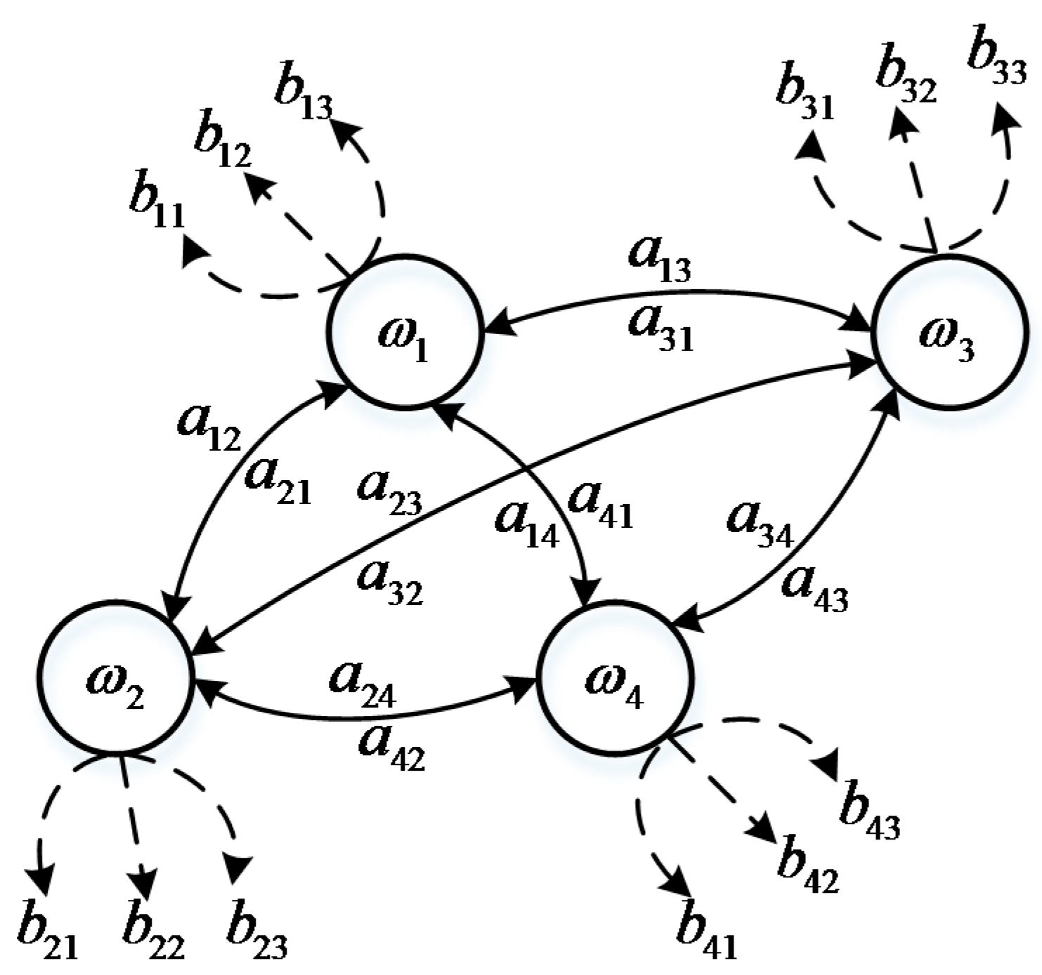
Assume that at moment t, a system is in state , and meanwhile the system activates a visible symbol . A specific time series would activate a specific series of visible symbols: . In this Markov model, state is invisible, but the activated visible symbol can be observed. We define this model as a finite state machine (FSM), shown in Figure 2. The activation probability of a FSM is defined by Equation (2):
In this equation, we can only observe the symbol . In Figure 2 it can be seen that the FSM has four invisible states linked with transfer probabilities and each of them can activate three different visible symbols. The FSM is strictly subject to causality, which means the probability in the future conclusively depends on the current probability.
2.3. Baum-Welch Algorithm
The Baum-Welch algorithm [38] is used in estimation. Transfer probabilities and activation probabilities are from a pool of training samples. The normalized premise of and is that:
We define a forward recursive equivalence in Equation (4), where denotes the probability in state at moment t which has generated t symbols of the sequence before. is the transfer probability from state to state and is the probability of activated symbol in state :
We define a backward recursive equivalence in Equation (5) either, where denotes the probability in state at moment t which generates symbols of the sequence from moment t + 1 to T. is the transfer probability from state to state and is the probability of activated symbol on state :
the parameters in the above two equations remain unknown, so an expectation maximized strategy can be used in the estimation. According to Equations (4) and (5), we define the transfer probability that is from state to state under the condition of observed symbol :
where is the probability of the symbol sequence generated through any possible state sequence. Expectation transfer probability through a sequence from state to state is and the total expectation transfer probability from state to any state is .
3. Data and Symbolization
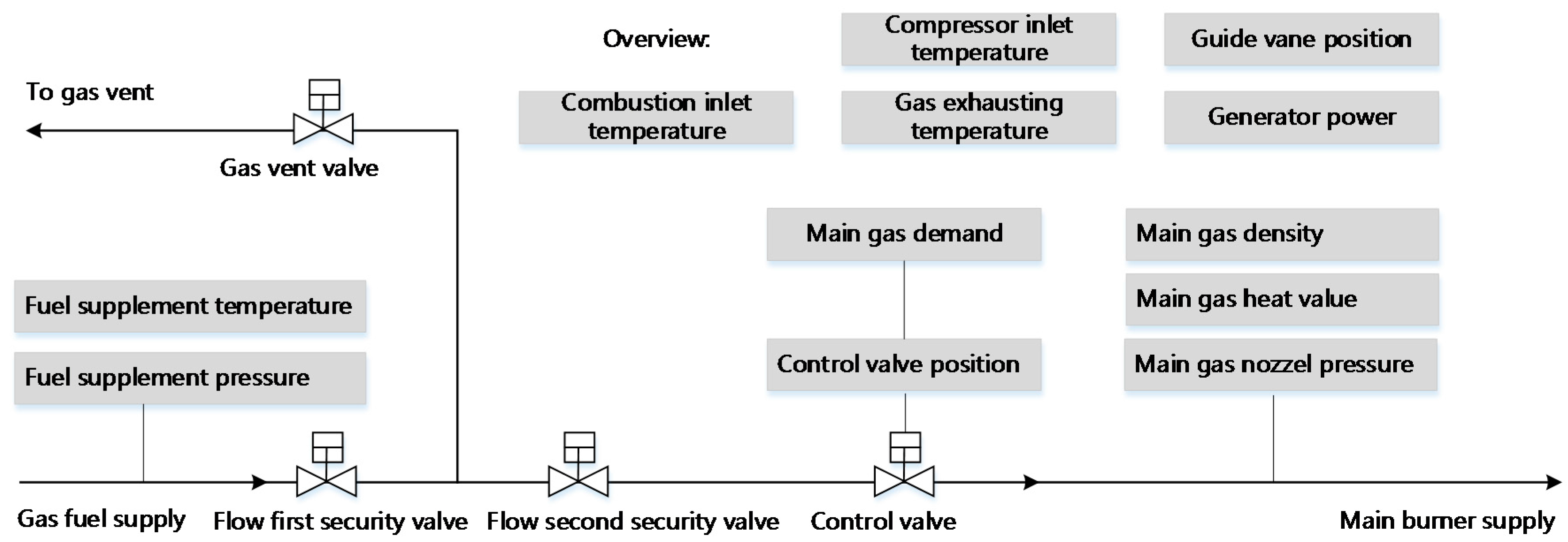
In gas turbine monitoring, all operation data observed by sensors are continuous. There is no observation that can acquire several discrete operating conditions automatically. Thus, in this section we focus on a symbol extraction method that can discretely represent different load condition patterns. After symbolization, many irrelevant interferences are dismissed. In this paper, the data resource is from a SOLAR, Titan 130 Gas Turbine. The parameters used are listed in Table 2 below and an overview of the structure of the turbine fuel system is shown in Figure 3.
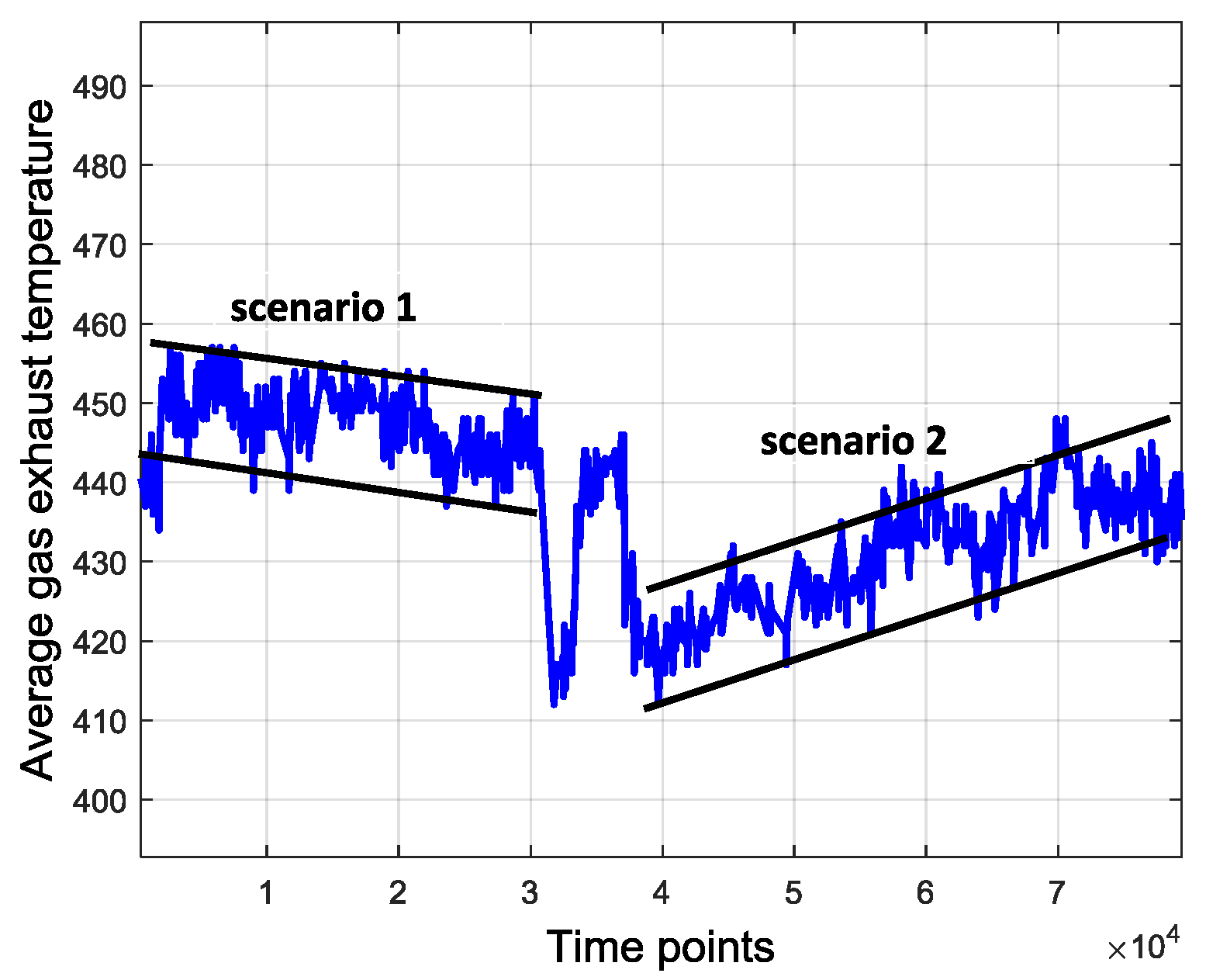
Original data contain many uncertainties and ambient disturbances. For example, the average combustion inlet temperature varies during daytime and at night, influenced by the atmospheric temperature that fluctuates over several days. This tendency is shown in Figure 4. Besides, the operating parameters of the gas turbine also have uncertainty, even under the same operating pattern. Figure 5 shows the uncertainty of the average gas exhaust temperature. It suggests that both in scenarios 1 and 2, the average gas exhaust temperature has an uncertainty boundary around the center line. All these factors may influence the device operation and data processing. The disturbances and uncertainties are usually extraneous and redundant, which interferes with the anomaly detection. Therefore, one way to eliminate such interferences is data symbolization.
Many strategies for data symbolization or discretization have been proposed and were well discussed in previous papers [39,40,41]. In summary, two kinds of approaches—splitting and merging—can be used in data symbolization. A feature can be discretized by either splitting the interval of continuous values or by merging the adjacent intervals [36]. It is very difficult to apply the splitting method in our study since we cannot properly preset the intervals. Therefore, a simple merging-based strategy is adopted for data symbolization. We apply a cluster method to symbol extractions—K means (KM) cluster method. The main reason is that in a FSM, the number of hidden states and visible symbols are both finite and KM initially has a specific cluster boundary and expected cluster numbers. Samples in a cluster are regarded as the same symbol. There are seven clusters that correspond to seven different load conditions as shown in Table 3, so K is equal to 7 for the KM model.
The purpose of the KM method is to divide original samples into k clusters, which ensures the high similarity of the samples in each cluster and low similarity among different clusters. The main procedures of this method are as follows:
- (1)
- Choose k samples in the dataset as the initial center for each cluster, and then evaluate distances between the rest of the samples and every cluster centers. Each sample will be assigned to a cluster to which the sample is the closest.
- (2)
- Renew the cluster center through the nearby samples and reevaluate the distance. Repeat this process until the cluster centers converge. Generally, distance evaluation uses the Euclidean distance and the convergence judgement is the square error criterion, as shown in Equation (7):where E is sum error of total samples, P is the position of the samples and is the center of cluster . Iteration terminates when E becomes stable, which is less than 1 × 10⁻⁶.
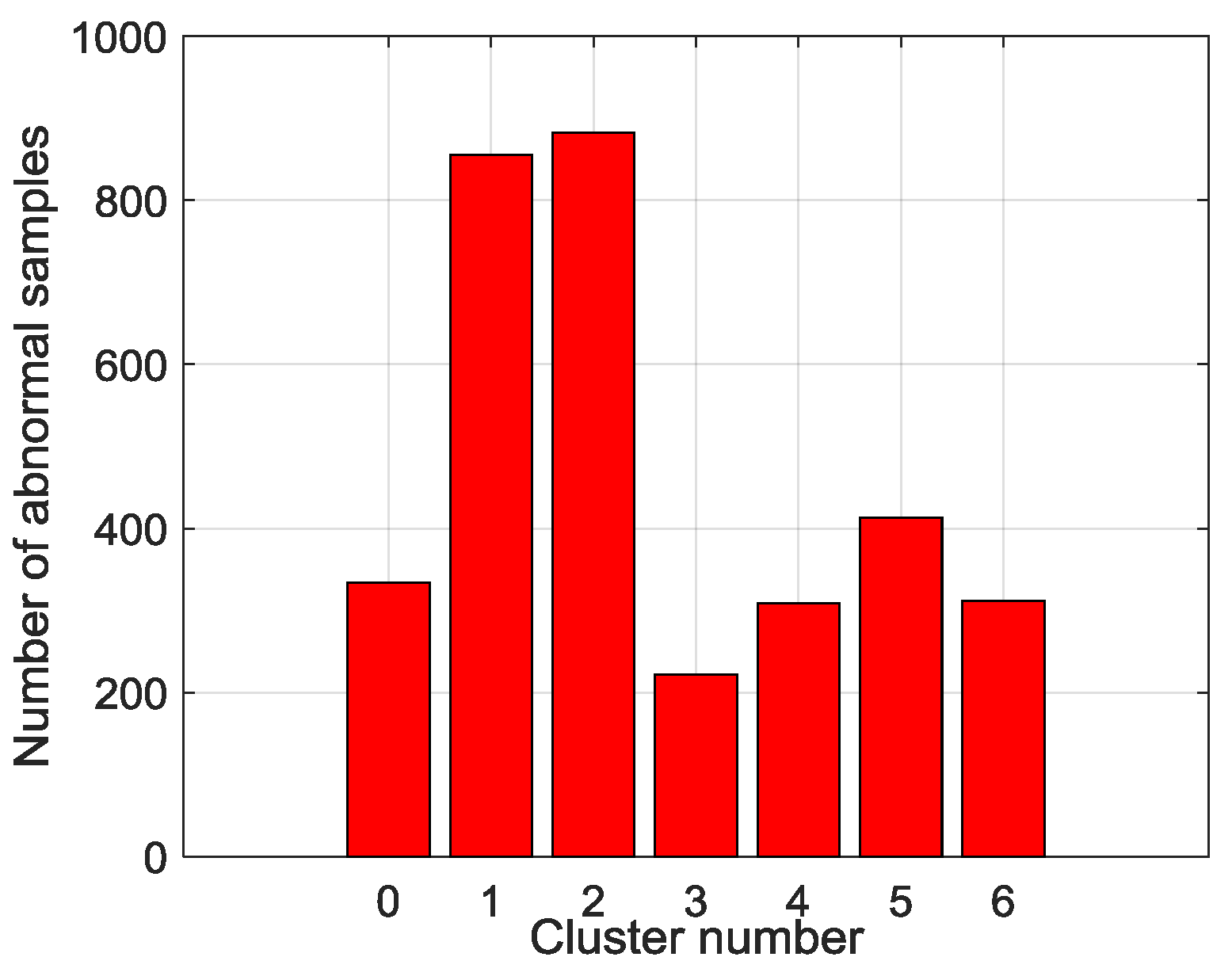
Therefore, the final clusters and samples are converted from continuous variables into discrete visible symbols. In this study, altogether 79,580 samples that are divided into seven symbols. The sampling interval is 10 min and symbol extraction results are shown in Figure 6. The most frequent symbols are Steady in high load (SHL) and Steady in low load (SLL). The intermediate ones are Flow rise in low load (FRLL), Flow rise in high load (FRHL), Flow drop in low load (FDLL) and Flow drop in high load (FDHL). The least frequent symbol is Fast changing condition (FCC). There are 3327 samples labeled as anomalies and the distribution of the abnormal samples is shown in Figure 7. All of the abnormal labels are derived manually from the device operation logs and maintenance records. To simplify our modeling, we classify all kinds of anomalies or defects in records into one class—anomaly. After symbolization, we use these symbols generated by KM cluster method to construct a FSM to measure whether a series of symbols are on normal conditions or on an abnormal one.
4. FSM Modeling and Anomaly Detection Methods
The finite state machine, widely applied in symbolic dynamic analysis, has shown great superiority in comparison to other techniques [30,31]. Therefore, the main tasks of establishing a sequential symbolic model in gas turbine fuel system anomaly detection are to build a FSM to estimate posterior probabilities of sequences and to build detection models to detect the abnormality of sequences. Before this, however, the discrete symbols extracted in Section 3 need to be sequenced into series, time series segments, of length T.
For FSM modeling, one aspect of this work is to determine several parameters. There are five states defined in this model: normal state (NS), anomaly state (AS), turbine startup (ST+), turbine shutdown (ST-) and halt state (HS). Actually, anomaly is a hidden state that is usually invisible during operation compared to the other four states. Till now, we have defined the model structure of the FSM which contains five states and seven visible symbols. For any moment, there are seven possible symbols in a state that could be observed with probability . is the probability that a state transfers from one to another. When the operating pattern changes reflected by symbols or hidden states at a structural level, the device might experience an anomaly that is easier to observe. This thus satisfies the basic idea of anomaly detection, finding patterns in data that do not conform to expected behavior.
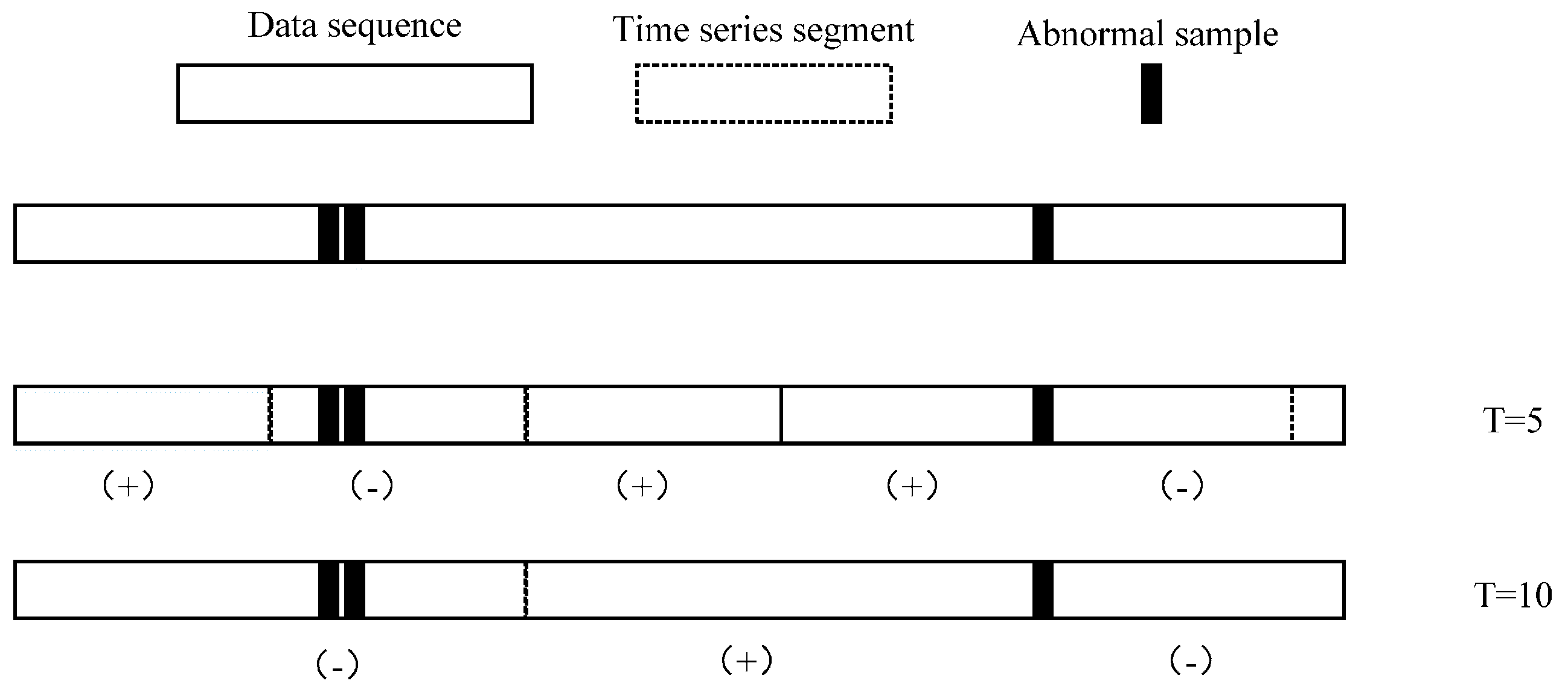
Another concern about FSM modeling is how long the time series are, which can be efficiently involved in the transfer and activation probability estimation. Figure 8 shows that different lengths T of segments may lead to different classification label results. A segment is defined as an anomaly only if it contains at least one abnormal sample. This classification suggests that the time series in T = 5 and T = 10 are significantly different.
It is difficult to primordially define a proper T that can be applied well in parameter estimation and anomaly detection, so another way we take is to optimize length T recursively until it has the best performance in the anomaly detection section. We declare that in actual data preprocessing, time series are generated by a sliding window with length T in order to ensure that the size of time series can match the original dataset, which means the total number of time series is 79581-T.
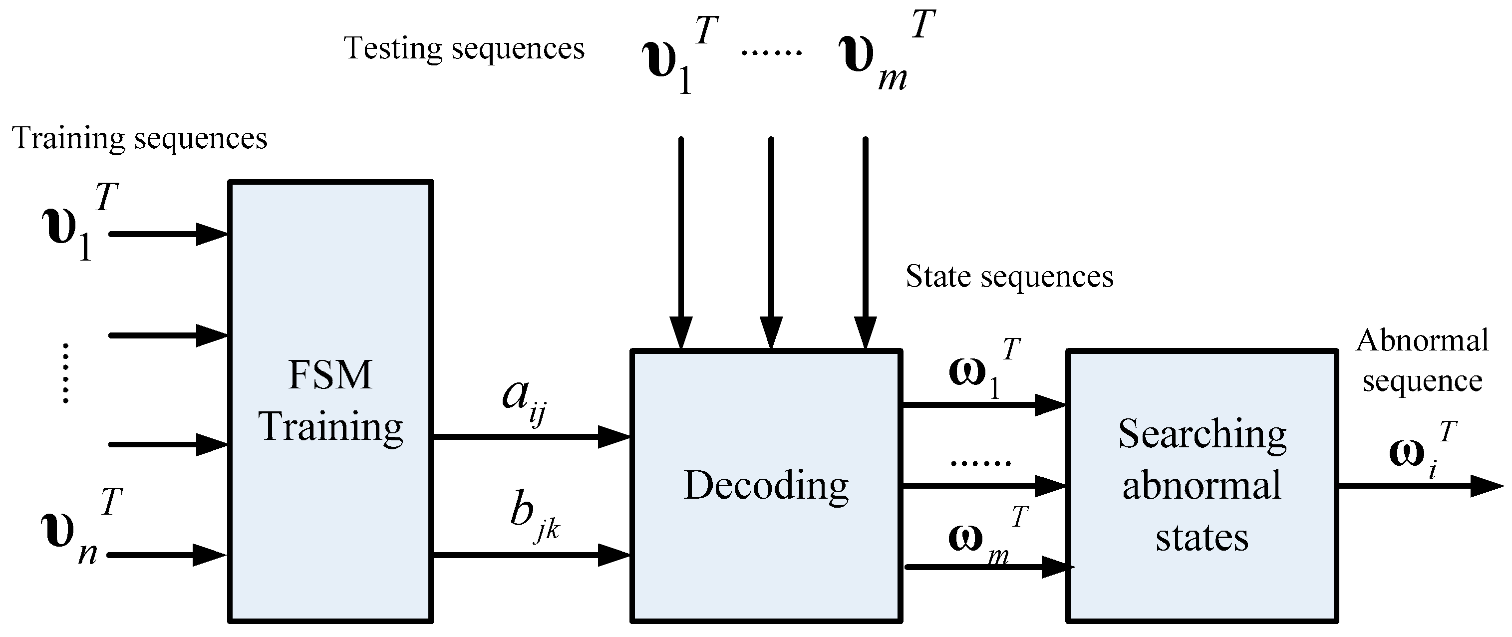
For anomaly detection, two strategies are used: an estimation-based model and a decoding-based model. The estimation-based model is that we use FSM to calculate the probability of a symbol sequence. In this case, FSM is built by the training data precluding abnormal samples, so the abnormal sequences contained in the testing data will have very low probabilities through calculation. The decoding-based model is that we use a FSM to decode a most probable state sequence which generates an observed symbol sequence. If the estimated state sequence contains anomaly states (AS), the symbol sequence is judged to be an anomaly.
According to the aforementioned contents, the schematic of a FSM modeling is shown in Figure 9, as illustrated below. First, data are sequenced into a pool of time series by an initial sliding window with length T. Then data are divided into two parts: training data and testing data. The training data are used to construct a FSM, to estimate transfer and activation probabilities of unknown states and visible symbols. The testing data are used to evaluate the FSM performance. After modeling the FSM, performance will be tested through two anomaly detection strategies—the decoding-based model and the estimation-based model. Length T will be updated until the models and the FSM achieve the best performance.
4.1. Training a FSM
The main task of training a FSM is to estimate a group of transfer probabilities and activation probabilities from a pool of training samples. In this study, Baum-Welch algorithm [41] is used in estimation. The probability is deduced in Equation (6). Therefore, an estimated transfer probability is described as:
Similarly, estimation of activation probability is described as:
where expectation activation probability of on state is and the total expectation activation probability on state is , l is number of symbols.
According to the analysis above can be gradually approximated by through Equations (8) and (9) until convergence. The pseudocode of the estimation algorithm is shown in Algorithm 1 below. The first are generated randomly at the beginning. Hence we can evaluate using estimated in the former generation. We repeat this process until the residual between and is less than a threshold and then the optimized are used in the FSM.
| Algorithm 1. Procedures of estimation. | |
| Input: | |
| Initial parameters , Training set , convergence threshold , | |
| Output: | |
| Finial estimated FSM parameters | |
| 1 | Loop |
| 2 | Estimating by in Equation (8) |
| 3 | Estimating by in Equation (9) |
| 4 | |
| 5 | |
| 6 | Until |
| 7 | Return , |
4.2. Anomaly Detection Based on the Estimation Strategy
An estimation strategy is used in anomaly detection of FSM in this part, which is inspired by anomaly detection approaches. Anomaly detection is defined as finding anomalous patterns in which data do not relatively satisfy expected behavior [22]. The FSM estimation strategy calculates the posterior probabilities of the symbol sequences generated by FSM. It can detect anomalies efficiently if it has been built from normal data. Therefore, this strategy conforms to the basic idea of what anomaly detection does. In this strategy, FSM is utilized to establish an expected pattern and the estimation process involves finding the nonconforming sequences, in other words, the anomalies. Figure 10 illustrates the schematic of anomaly detection using the estimation strategy. In order to establish an expected normal pattern, the training data used in FSM modeling are utterly normal sequences. Parameters are estimated by FSM training, which indicates the intrinsic normal pattern recognition capability contained in these parameters, hence, the model estimation probabilities of testing symbol sequences in which abnormal sequences are included. Probabilities in normal sequences will be much higher than that in abnormal ones, so the detection indicator is actually a preset threshold that judges the patterns of test sequences.
The probability of a symbol sequence generated by a FSM can be described as:
where r is the index of state sequence of length T, . If there are, for instance, c different states in this model, the total number of possible state sequences is . An enormous amount of possible state sequences need to be considered to calculate the probability of a generated symbol sequence , as shown in Equation (10). The second part of the equation can be descried as:
The probability is continuous and chronological multiplication. Assume that activation probability of a symbol critically depends on the current state, so the probability can be described in Equation (12) and then Equation (13) is the other description of Equation (10):
However, the computing cost of the above equation is which is too high to finish this process. There are two alternative methods that can dramatically simplify the computing process, a forward algorithm and a backward algorithm, which are depicted by Equations (5) and (6), respectively. The computing cost of these algorithms are both , that is times faster than the original strategy. Algorithm 2 shows the detection indicator based on the forward algorithm. Initialize , training sequences precluding anomalies, , t = 0., then update until t = T and the probability of is . If the probability is higher than the preset threshold, then the symbol sequence is classified in the positive, normal class. Otherwise the symbol sequence is classified in the negative, anomalous class.
| Algorithm 2. Anomaly detection based on the estimation strategy. | |
| Input: | |
| , , sequence , , threshold | |
| Output: | |
| Classification result | |
| 1 | For |
| 2 | |
| 3 | Until |
| 4 | Return |
| 5 | If |
| 6 | |
| 7 | Else |
| 8 | Return |
There are two points to be mentioned. In the first place, the decision judgement is very simple for use of anomaly detection by threshold . This convenience is ascribed to the normal pattern constructed by FSM. The probabilities estimated from FSM intuitively simulate the possibilities of the symbol sequences emerging in a real system. Furthermore, the performance of this strategy is not only dependent on the efficiency of the trained FSM, but also on the proper threshold. Therefore, in the modeling process, we optimize the threshold by traversing different values in order to get the highest overall accuracy of normal and abnormal sequences.
4.3. Anomaly Detection Based on the Decoding Strategy
Compared to the estimation strategy, a FSM can detect anomalies too if it can recognize whether there are hidden anomalous states in sequences. Fortunately decoding a state sequence is available in FSM so another way to detect anomalies is to decode a symbol sequence to state sequence and then find whether the state sequence contains abnormal states. Unlike the previous estimation strategy, the decoding strategy is a sort of, somehow, optimization algorithm in which a searching function is used. Figure 11 illustrates the schematic of anomaly detection using the decoding strategy. In this strategy, FSM is trained by all sequences that contain both normal and abnormal sequences so the FSM reflects the system that may run on normal or abnormal patterns. After that, the decoding process involves searching for the most probable state sequence that the symbol sequence corresponds to. A greedy-based method is applied in searching in each step so the most possible state is chosen and is added to the path. The final path is the decoded state sequence. Finally, the model judges a symbol sequence by its state sequence on whether it contains anomaly states.
Algorithm 3 shows the procedures of the decoding-based anomaly detection strategy. Initialize parameters , testing sequence , , and path. Then, update and in each moment t, traverse all state candidates and the most possible state in this moment is the one who makes biggest and then add the state into the path until the end of the sequence. After that, scan the decoded state sequence if there is at least one anomaly state (AS), then the observed sequence is classified in the negative, anomalous class, otherwise classified in the positive, normal class.
| Algorithm 3. Anomaly detection based on the decoding strategy. | |
| Input: | |
| , , , , | |
| Output: | |
| Classification result | |
| 1 | For |
| 2 | |
| 3 | For |
| 4 | |
| 5 | Until |
| 6 | |
| 7 | Add to |
| 8 | Until |
| 9 | If contains state (AS) |
| 10 | |
| 11 | Else |
| 12 | Return |
Compared to the estimation strategy, the decoding strategy has some advantages and disadvantages. First of all, the detection indicator based on the decoding strategy may help the anomaly detection system sensitivity improve, meaning that it can precisely warn of an anomaly once it occurs. Besides, it helps system locate anomaly emerging time in high resolution. For example, a sequence contains 10 samples and the sample interval is 10 min so the length of the sequence is 100 min. If the sequence is abnormal and the two system, estimation-based model and decoding-based model, both alert, the latter can provide a more precise anomaly occurrence time, for instance, in 20 min and 60 min possibly but the former can only provide a probability that an anomaly may have occurred. However, this point may also be a disadvantage of the decoding strategy due to the lack of robustness. This detection strategy is a local optimization algorithm that may reach a local minimum point that is actually not the global optimized solution. It may have searched an utterly different state sequence than the real one. Furthermore, error rate accumulates with the growth of the searching path, particularly for a longer length T, and the false positive rate may be very high, meaning that many normal sequences are classified as anomalies, so the length of the sequence is a critical factor for detection performance. It indicates the robustness performance of the models. This issue will be analyzed in the next section.
5. Experimental Design and Results Analysis
5.1. Performance Evaluation
The data used in this section is from a SOLAR Titan 130 gas turbine power generator on an offshore oil platform. The data list and symbol distribution are shown in Table 2 and Figure 6. Overall (79581-T) sequences are used in training and testing by cross validation. The dataset was divided equally and sequentially into ten folders. Each folder was used in turn as testing data, with the other nine as training data, until every folder had been tested by the others. Hence the final result consists of a performance average together with a standard deviation.
The labels of the samples are grouped into positive (normal) and negative (anomaly). The detection performance is measured by the true positive rate (TP rate) and true negative rate (TN rate) [42]. Table 4 shows the definition of confusion matrix which measures four possible outcomes.
The TP rate is defined as the ratio of the number of samples correctly classified as positive to the number of samples that are actually positive:
The TN rate represents the ratio of the number of samples correctly classified as negative to the number of actual negative samples:
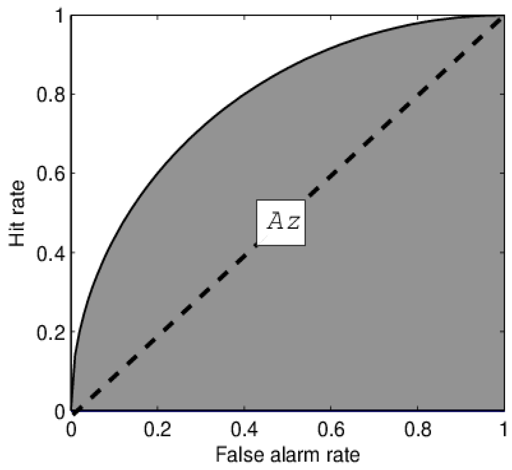
In this paper, anomaly detection on a gas turbine fuel system is a class imbalanced problem in that the normal class is much larger than the abnormal class. The performance of imbalanced data can be measured by AUC, which is the area under the Receiver Operating Characteristic (ROC) curve, as shown in Figure 12. The ROC curve is a plot of the FP rate on the X axis versus the TP rate on the Y axis. It shows the differences between the FP rate and the TP rate based on different rules.
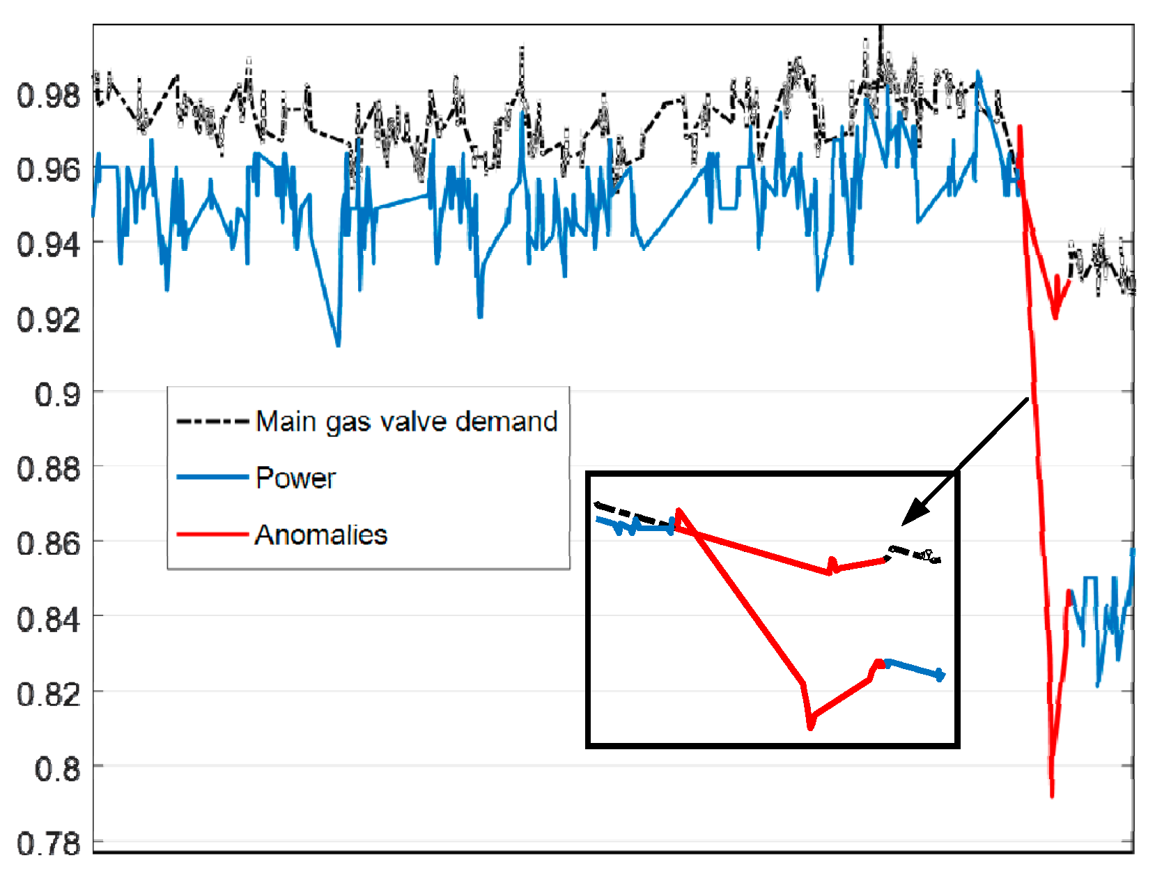
5.2. Exemplary Cases and Experimental Results
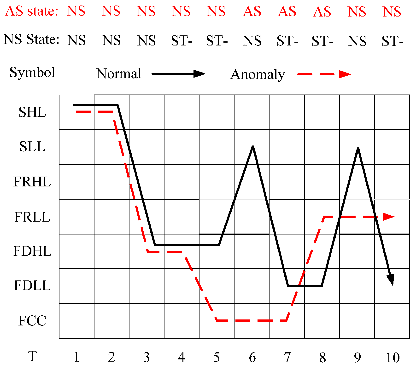
To illustrate how the detection system works, two exemplary cases are provided. One is a normal sequence. Another is an abnormal sequence that is in fuel nozzle valve anomaly, which may cause the fuel flow fluctuation or drop and in turn cause a load drop. The selected sequences, after normalization, are of length T = 10, with a 10 min sampling interval, for a total 100 min. The anomalous sequence is shown in Figure 13 as the red sequence, for original parameters ‘Main gas valve demand’ and ‘Power’. The two sequences, partitioned into symbols, are described in Figure 14. The routine map is consisted of seven different symbols and 10 time points. The black row is the normal sequence and the red dashed line is the anomalous sequence. Besides, the labeled state sequence of normal and anomalous cases are {NS, NS, NS, ST-, ST-, NS, ST-, ST-, NS, ST-}.and {NS, NS, NS, NS, NS, AS, AS, AS, NS, NS}, respectively.
The results are generated by the trained FSM and the two detection models, the estimation- and decoding-based models. Threshold in this model is 0.00743 and the posterior probabilities of normal and anomalous sequences determined by the estimation-based model are 0.01563 and 0.0009235. The decoded most probable state sequences calculated by the decoding-based model are {NS, NS, NS, NS, ST-, ST-, ST-, NS, ST-, NS} and {NS, NS, NS, NS, NS, AS, AS, AS, AS, NS}. The anomalous sequence contains AS, yet the normal doesn’t. As a result, these two models have both made correct decisions. The performance of the two models in each data group within the cross-validation is given in Table 5. It can be seen from the table that the overall performance of the estimation-based model is better than that of the decoding-based model. Specifically, the estimation-based model’s evaluation in eight groups for TP rate, six groups for TN rate and eight groups for AUC are better than the other model. Similarly, Table 6 and Table 7 show the evaluation of the confusion matrixes for the two models. The results illustrate that the estimation-based model outperforms the decoding-based model in overall accuracy as well as deviation. Therefore, it can be concluded that in terms of T = 10, = 0.00743, the estimation-based model can resolve anomaly detection in gas turbine fuel systems more efficiently. However, as analyzed earlier, the threshold and length of sequence can drastically influence detecting performance. As a result, several impacts need to be further discussed.
5.3. Threshold Determination Strategy
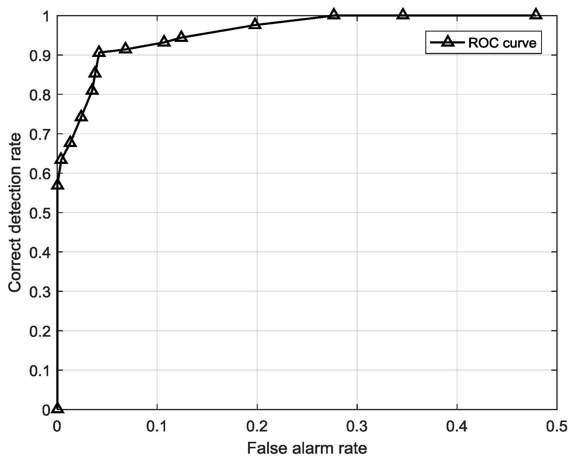
Aside from training a FSM, a core problem of building an estimation-based detection model is to determine a proper threshold . In a particular sequence length, we can find a most suitable value that can classify the testing sequence well. Actually, with different thresholds, we will gain different classification results, as is shown in Figure 15, which is a ROC curve of the estimation-based model with different thresholds. The optimized threshold is one of them on the curve.
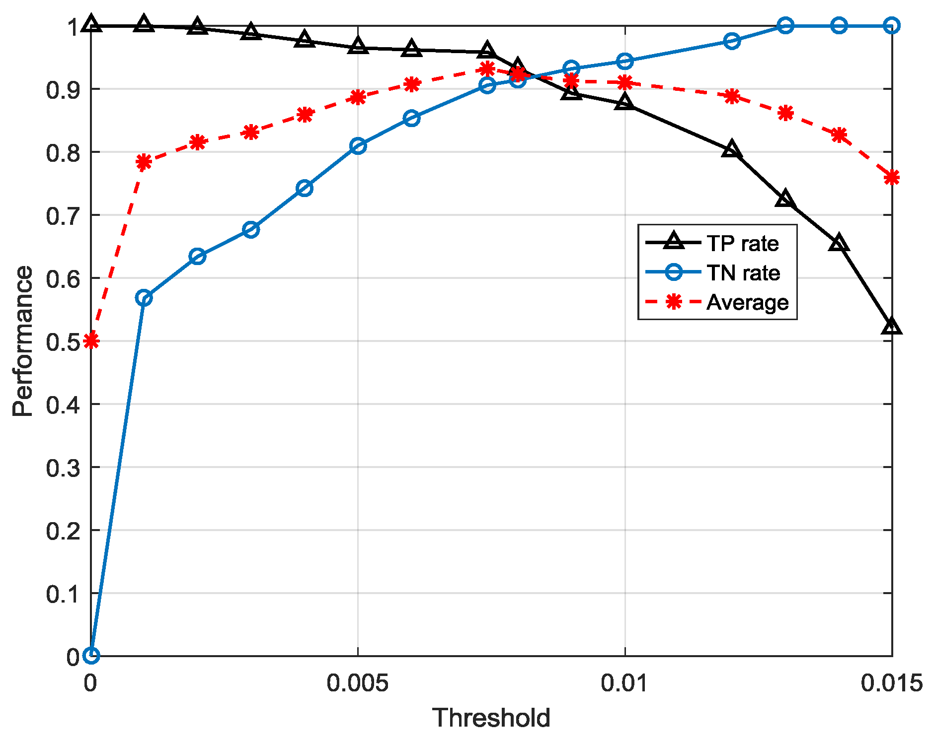
A sequence is judged to be anomalous when its posterior probability is less than . When = 0, the TN rate, the correct detected anomalous sequence among all anomalies, is 0 initially. Then the TN rate increases with the growth of to 1 when reaches a certain point. On the contrary, the TP rate is 1 initially when = 0 since all the posterior probabilities are over 0. Then the TP rate starts to decrease with the growth of . This regularity is illustrated in Figure 16. One concern is that both the TP rate and TN rate are important for the model performance, so the most suitable threshold should be found in a synthesized highest place, which is measured by the average accuracy that is the mean value of the TP rate and TN rate. In this experiment, we searched the in step of 0.0001 until it reached the peak average accuracy when = 0.0074.
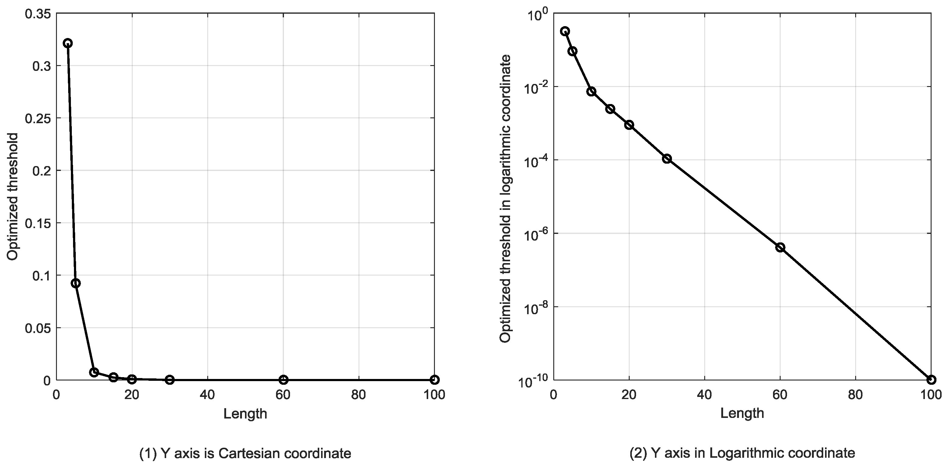
The optimized threshold will drop along with the change of length T because the posterior probabilities are continuously multiplying. The probabilities drop exponentially as T increases. Figure 17 shows optimized thresholds for different sequence lengths.
5.4. Comparison between the Two Models on Different Length of Sequence
Another main factor that influences the performance of the detection models with the length of sequence. The robustness performance of the two models are measured by AUC for different sequence lengths. A model with high robustness performance will have a relatively stable AUC with the growth of length T, and vice versa.
Figure 18 and Figure 19 illustrate the comparison between the estimation-based model and decoding-based model in TN rate and TP rate for different lengths of sequence, respectively. With the growth of length, the TN rate and TP rate of estimation-based model gradually decrease and then become stable after about T > 60, steadying in 0.82 in TN rate and 0.89 in TP rate. However, the performance of the decoding-based model seems different to that of the estimation-based model. The TN rate of the decoding-based model rises to nearly 1 when the length T > 30, whereas the TP rate decreases drastically when T > 20. The tremendous difference between the two models is ascribed to several reasons. First, the detection mechanisms of the two models are not confirmed. The estimation-based model is built upon the premise of a normal pattern which is constructed by a normal pattern based FSM, while the decoding-based model is built upon the trained FSM containing normal and anomalous sequences. It points out that estimation-based model concerns those data without anomalies while the decoding-based model concerns all the data whatever class they belong to. Second, the detection indicator used in the estimation-based model is posterior probabilities whereas the detection indicator used in the decoding-based model is states. With the growth of length T, the sequences become longer and more complicated for classification using a threshold because there are more single symbols in a sequence. As a result, the performance of the estimation-based model decreases and eventually becomes steady because of a suitable threshold and classification capability of FSM. Regarding the decoding-based model, it is more complicated than the estimation-based model. With the growth of length T, the sequences become longer, but it is easier to find a possible abnormal state. A sequence is judged to be anomalous only if there is at least one abnormal state. The longer the sequence is, the more probable it is that abnormal states will hide, so the TN rate rises when the length is growing. On the contrary, it is easy to understand that long, complicated sequences would lead to the model’s incorrect judgement because the more states to be decoded, the higher the possible of misjudgement, so the TP rate decreases along with the growth of T.
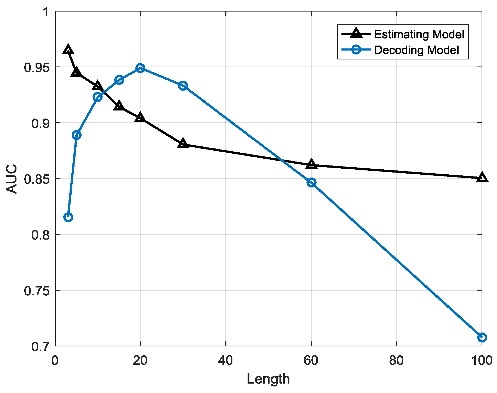
Based on the points presented above, we can draw the following conclusion: the estimation-based model has a better robustness performance than the decoding-based model while the decoding-based model may yield better performance in particular intervals. Figure 20 shows the AUC comparison between the estimation-based model and decoding-based model, which is an evaluation measurement that reflects the overall classification performance of a model for class imbalanced problems. The AUC of the estimation-based model gradually decreases as the TP rate and TN rate along with the growth of length T. However, the AUC of the decoding-based model rises to a peak value when T = 20 and then starts to drop. In this figure, we can see that before T = 12, the performance of the estimation-based model is better than that of the decoding-based model. Between T = 12 and 53, the decoding-based model outperforms the estimation-based model. After T > 53, the estimation-based model is much more efficient than the decoding-based model. In conclusion, if we need a short term anomaly detection system, e.g., with less than a 1 h observation window, the estimation-based model will be satisfactory. If a long term anomaly detection system is needed, e.g., for 1 h to 8 h, then the decoding-based model will be more efficient. For an ultra-long term anomaly detection system, e.g., over 8 h, an estimation-based model should be used.
The main reason that causes the difference between the two models is that in the estimation-based model, FSM is used to calculate posterior probabilities for normal sequences, so it is trained by completely normal data. When FSM are calculating probabilities for testing sequences that are anomalous data, the results would be much lower than that of normal data. Therefore, optimizing a proper threshold classifying two classes would be of great use for an efficient model performance. In the decoding-based model, FSM is used to find the most probable state sequence of an observed sequence. The main task of FSM is to detect anomalous states efficiently so it is trained by both normal and abnormal data. Once an anomalous state is detected, the sequence is judged to be an anomaly.
5.5. Comparison of the Different Models
In this Section, four models are compared to our proposed models, which are the fuzzy logic method (FL) [21], extended Kalman filtering (EKF) [43], support vector machine (SVM) [14] and back propagation network (BPN) [12]. Fuzzy set theory and fuzzy logic provide the framework for nonlinear mapping. Fuzzy logic systems have been widely used in engineering applications, because of the flexibility they offer designers and their ability to handle uncertainty. Extended Kalman filtering is widely used in state estimation and anomaly detection. It uses measurable parameters to estimate operating state by state functions and measurement functions for 1-D non-linear filtering. Supported vector machine is an algorithm that emphasizes structural risk minimization theory. An SVM can operate like a linear model to obtain the description of a nonlinear boundary of a dataset using a nonlinear mapping transform. The perceptron learning rule is built by a hyperplane alone, with a group of weights assigned to each attribute. Data are classified into one class when the sum of the weights of an attribute is a positive number and into another class when the sum is a negative number. In the back-propagation network, attributes are reweighted if the samples are classified incorrectly until the classification is correct.
The four models can be divided in two categories: fuzzy logic and extended Kalman filtering are model-based approaches, and support vector machine and back propagation network are machine learning-based approaches. The estimation-based model (EBFSM) and decoding-based model (DBFSM) are in sequential length T = 10. The overall accuracy is AUC instead. The experimental result is shown in Table 8. It can be seen that the proposed models have a better performance than any other compared models, though the compared four models have similar performance. Concretely, in 10 different datasets, the estimation-based model outperforms the compared models in nine groups and the decoding-based model outperforms the compared models in eight groups. The two proposed models have about 3–5% higher accuracy than any other models.
6. Conclusions
The essential issue of anomaly detection is how to detect sensitively and effectively when and how an anomaly would happen. Conventional anomaly detection methods for points or collective anomalies are mostly established based on continuous real-time sensor observations. Noise, operating fluctuation or ambient conditions may be all contained in raw data, which make anomalous observations appear normal. The anomalous features often hide in the structural data which reflects various patterns of the device operating. Thus, we first partitioned the original data into classes by using K-means clustering and symbolized each class to construct a sequence-based feature-structure which intrinsically represents the operating patterns of a device. Second, we built the core computing unit for anomaly detection, finite state machine, on a large quantity of training sequential data to estimate posterior probabilities or find most probable states. Two detection models were generated, an estimation-based model and decoding-based model. The two models on anomaly detection for gas turbine fuel system have their own advantages and weakness, concretely concluded as follows:
- (1)
- The estimation-based model has strong robustness since the performance is highly stable when the sequence length is growing. However, in the decoding-based model, the performance varies with different sequence lengths. The anomalous sequences are easier to detect in longer lengths than in shorter one, but there will be a higher false alarm rate at longer lengths, which means many normal sequences are misclassified as anomalies.
- (2)
- The decoding-based model can help us to locate anomalies occurring point with a high time resolution, which means it can tell us precisely what symbol points are in an anomalous state rather than only probabilities of sequences made by the estimation-based model.
The estimation-based model is more suitable for anomaly detection in gas turbine fuel systems when the observation window is less than 1 h or over 8 h, whereas the decoding-based model is more suitable when the observation window is between 1 and 8 h, so it may help people choose the most efficient detection model for different demands.
Further work may be concentrated on algorithm optimization and application extension. As is described above, the decoding-based model uses a local searching algorithm which may cause high deviation in some circumstances, though it could be operated at a high computing speed, so the algorithms need to be optimized. We also need to apply this method to other domains of gas turbine anomaly detection, such as gas path, combustion components, etc. All of these need further attention.
Acknowledgments
This paper was partially supported by National Natural Science Foundation of China (NSFC) grant U1509216, 61472099, National Sci-Tech Support Plan 2015BAH10F01, the Scientific Research Foundation for the Returned Overseas Chinese Scholars of Heilongjiang Province LC2016026 and MOE–Microsoft Key Laboratory of Natural Language Processing and Speech, Harbin Institute of Technology.
Author Contributions
Fei li developed the idea, performed the experiments and wrote the draft paper. Hongzhi Wang reviewed and supervised the whole paper. Guowen Zhou got involved in data processing and experimental analysis, Daren Yu and Jiangzhong Li significant improved the paper in scientific ideas and helped modify the paper. Hong Gao provided the raw data and involved in data preprocessing and improved the paper from algorithmic perspective.
Conflicts of Interest
The authors declare no conflict of interest.
References
- Volponi, A.J. Gas Turbine Engine Health Management: Past, Present and Future Trends. In Proceedings of the ASME Turbo Expo 2013: Turbine Technical Conference and Exposition, San Antonio, TX, USA, 3–7 June 2013; pp. 433–455. [Google Scholar]
- Marinai, L.; Probert, D.; Singh, R. Prospects for Aero Gas-Turbine Diagnostics: A Review. Appl. Energy 2004, 79, 109–126. [Google Scholar] [CrossRef]
- Urban, L.A. Gas Path Analysis Applied to Turbine Engine Condition Monitoring. J. Aircr. 1973, 10, 400–406. [Google Scholar] [CrossRef]
- Pu, X.; Liu, S.; Jiang, H.; Yu, D. Sparse Bayesian Learning for Gas Path Diagnostics. J. Eng. Gas Turbines Power 2013, 135, 071601. [Google Scholar] [CrossRef]
- Doel, D.L. TEMPER—A Gas-Path Analysis Tool for Commercial Jet Engines. J. Eng. Gas Turbines Power 1992, 116, V005T15A013. [Google Scholar]
- Gulati, A.; Zedda, M.; Singh, R. Gas Turbine Engine and Sensor Multiple Operating Point Analysis Using Optimization Techniques. In Proceedings of the AIAA/ASME/SAE/ASEE Joint Propulsion Conference and Exhibit, Las Vegas, NV, USA, 24–28 July 2000; pp. 323–331. [Google Scholar]
- Mathioudakis, K. Comparison of Linear and Nonlinear Gas Turbine Performance Diagnostics. J. Eng. Gas Turbines Power 2003, 127, 451–459. [Google Scholar]
- Stamatis, A.; Mathioudakis, K.; Papailiou, K.D. Adaptive Simulation of Gas Turbine Performance. J. Eng. Gas Turbines Power 1989, 238, 168–175. [Google Scholar]
- Meskin, N.; Naderi, E.; Khorasani, K. Nonlinear Fault Diagnosis of Jet Engines by Using a Multiple Model-Based Approach. J. Eng. Gas Turbines Power 2011, 13, 63–75. [Google Scholar]
- Kobayashi, T.; Simon, D.L. Evaluation of an Enhanced Bank of Kalman Filters for In-Flight Aircraft Engine Sensor Fault Diagnostics. J. Eng. Gas Turbines Power 2004, 127, 635–645. [Google Scholar]
- Doel, D. The Role for Expert Systems in Commercial Gas Turbine Engine Monitoring. In Proceedings of the ASME 1990 International Gas Turbine and Aeroengine Congress and Exposition, Brussels, Belgium, 11–14 June 1990. [Google Scholar]
- Loboda, I.; Feldshteyn, Y.; Ponomaryov, V. Neural Networks for Gas Turbine Fault Identification: Multilayer Perceptron or Radial Basis Network? In Proceedings of the ASME 2011 Turbo Expo: Turbine Technical Conference and Exposition, Vancouver, BC, Canada, 6–10 June 2011. [Google Scholar]
- Bettocchi, R.; Pinelli, M.; Spina, P.R.; Venturini, M. Artificial Intelligence for the Diagnostics of Gas Turbines—Part I: Neural Network Approach. J. Eng. Gas Turbines Power 2007, 129, 19–29. [Google Scholar] [CrossRef]
- Lee, S.M.; Choi, W.J.; Roh, T.S.; Choi, D.W. A Study on Separate Learning Algorithm Using Support Vector Machine for Defect Diagnostics of Gas Turbine Engine. J. Mech. Sci. Technol. 2008, 22, 2489–2497. [Google Scholar] [CrossRef]
- Lee, S.M.; Roh, T.S.; Choi, D.W. Defect Diagnostics of SUAV Gas Turbine Engine Using Hybrid SVM-Artificial Neural Network Method. J. Mech. Sci. Technol. 2009, 23, 559–568. [Google Scholar] [CrossRef]
- Romessis, C.; Mathioudakis, K. Bayesian Network Approach for Gas Path Fault Diagnosis. J. Eng. Gas Turbines Power 2004, 128, 691–699. [Google Scholar]
- Lee, Y.K.; Mavris, D.N.; Volovoi, V.V.; Yuan, M.; Fisher, T. A Fault Diagnosis Method for Industrial Gas Turbines Using Bayesian Data Analysis. J. Eng. Gas Turbines Power 2010, 132, 041602. [Google Scholar] [CrossRef]
- Li, Y.G.; Ghafir, M.F.A.; Wang, L.; Singh, R.; Huang, K.; Feng, X. Non-Linear Multiple Points Gas Turbine Off-Design Performance Adaptation Using a Genetic Algorithm. J. Eng. Gas Turbines Power 2011, 133, 521–532. [Google Scholar] [CrossRef]
- Ganguli, R. Application of Fuzzy Logic for Fault Isolation of Jet Engines. J. Eng. Gas Turbines Power 2003, 125, V004T04A006. [Google Scholar] [CrossRef]
- Shabanian, M.; Montazeri, M. A Neuro-Fuzzy Online Fault Detection and Diagnosis Algorithm for Nonlinear and Dynamic Systems. Int. J. Control Autom. Syst. 2011, 9, 665. [Google Scholar] [CrossRef]
- Dan, M. Fuzzy Logic Estimation Applied to Newton Methods for Gas Turbines. J. Eng. Gas Turbines Power 2007, 129, 787–797. [Google Scholar]
- Chandola, V.; Banerjee, A.; Kumar, V. Anomaly Detection: A Survey. ACM Comput. Surv. 2009, 41, 1–58. [Google Scholar] [CrossRef]
- Lei, W.; Wang, S.; Zhang, J.; Liu, J.; Yan, Z. Detecting Intrusions Using System Calls: Alternative Data Models. In Proceedings of the 1999 IEEE Symposium on Security and Privacy, Oakland, CA, USA, 9–12 May 1999; pp. 133–145. [Google Scholar]
- Sun, P.; Chawla, S.; Arunasalam, B. Mining for Outliers in Sequential Databases. In Proceedings of the SIAM International Conference on Data Mining, Bethesda, MD, USA, 20–22 April 2006; pp. 94–106. [Google Scholar]
- Manson, G.; Pierce, G.; Worden, K. On the Long-Term Stability of Normal Condition for Damage Detection in a Composite Panel. Key Eng. Mater. 2001, 204–205, 359–370. [Google Scholar] [CrossRef]
- Ruotolo, R.; Surace, C. A Statistical Approach to Damage Detection through Vibration Monitoring. BMC Proc. 1997, 3, S25. [Google Scholar]
- Hollier, G.; Austin, J. Novelty Detection for Strain-Gauge Degradation Using Maximally Correlated Components. In Proceedings of the European Symposium on Artificial Neural Networks (ESANN 2002), Bruges, Belgium, 24–26 April 2002; pp. 257–262. [Google Scholar]
- Yairi, T.; Kato, Y.; Hori, K. Fault Detection by Mining Association Rules from Housekeeping Data. In Proceedings of the International Symposium on Artificial Intelligence Robotics & Automation in Space, St–Hubert, QC, Canada, 18–22 June 2001. [Google Scholar]
- Brotherton, T.; Johnson, T. Anomaly Detection for Advanced Military Aircraft Using Neural Networks. In Proceedings of the Aerospace Conference, Big Sky, MT, USA, 10–17 March 2001. [Google Scholar]
- Aminyavari, M.; Mamaghani, A.H.; Shirazi, A.; Najafi, B.; Rinaldi, F. Exergetic, Economic, and Environmental Evaluations and Multi-Objective Optimization of an Internal-Reforming SOFC-Gas Turbine Cycle Coupled with a Rankine Cycle. Appl. Therm. Eng. 2016, 108, 833–846. [Google Scholar] [CrossRef]
- Mamaghani, A.H.; Najafi, B.; Casalegno, A.; Rinaldi, F. Predictive Modelling and Adaptive Long-Term Performance Optimization of an HT-PEM Fuel Cell Based Micro Combined Heat and Power (CHP) Plant. Appl. Energy 2016, 192, 519–529. [Google Scholar] [CrossRef]
- Ray, A. Symbolic Dynamic Analysis of Complex Systems for Anomaly Detection. Signal Process. 2004, 84, 1115–1130. [Google Scholar] [CrossRef]
- Rao, C.; Ray, A.; Sarkar, S.; Yasar, M. Review and Comparative Evaluation of Symbolic Dynamic Filtering for Detection of Anomaly Patterns. Signal Image Video Process. 2009, 3, 101–114. [Google Scholar] [CrossRef]
- Gupta, S.; Ray, A.; Sarkar, S.; Yasar, M. Fault Detection and Isolation in Aircraft Gas Turbine Engines. Part 1: Underlying Concept. Proc. Inst. Mech. Eng. Part G J. Aerosp. Eng. 2008, 222, 307–318. [Google Scholar] [CrossRef]
- Yamaguchi, T.; Mori, Y.; Idota, H. Fault Detection and Isolation in Aircraft Gas Turbine Engines. Part 2: Validation on a Simulation Test Bed. Proc. Inst. Mech. Eng. Part G J. Aerosp. Eng. 2008, 222, 319–330. [Google Scholar]
- Soumik, S.; Jin, X.; Asok, R. Data-Driven Fault Detection in Aircraft Engines with Noisy Sensor Measurements. J. Eng. Gas Turbines Power 2011, 133, 783–789. [Google Scholar]
- Sarkar, S.; Mukherjee, K.; Sarkar, S.; Ray, A. Symbolic Dynamic Analysis of Transient Time Series for Fault Detection in Gas Turbine Engines. J. Dyn. Syst. Meas. Control 2012, 135, 014506. [Google Scholar] [CrossRef]
- Baum, L.E.; Petrie, T. Statistical Inference for Probabilistic Functions of Finite State Markov Chains. Ann. Math. Stat. 1966, 37, 1554–1563. [Google Scholar] [CrossRef]
- Liu, H.; Hussain, F.; Tan, C.L.; Dash, M. Discretization: An Enabling Technique. Data Min. Knowl. Discov. 2002, 6, 393–423. [Google Scholar] [CrossRef]
- Tsai, C.J.; Lee, C.I.; Yang, W.P. A Discretization Algorithm Based on Class-Attribute Contingency Coefficient. Inf. Sci. 2008, 178, 714–731. [Google Scholar] [CrossRef]
- Gupta, A.; Mehrotra, K.G.; Mohan, C. A Clustering-Based Discretization for Supervised Learning. Stat. Probab. Lett. 2010, 80, 816–824. [Google Scholar] [CrossRef]
- Witten, I.H.; Frank, E.; Hall, M.A. Data Mining: Practical Machine Learning Tools and Techniques, Second Edition (Morgan Kaufmann Series in Data Management Systems). ACM Sigmod Rec. 2011, 31, 76–77. [Google Scholar] [CrossRef]
- Chen, J.; Patton, R.J. Robust Model-Based Fault Diagnosis for Dynamic Systems; Springer: New York, NY, USA, 1999. [Google Scholar]
Figure 1.
Discrete Markov model.
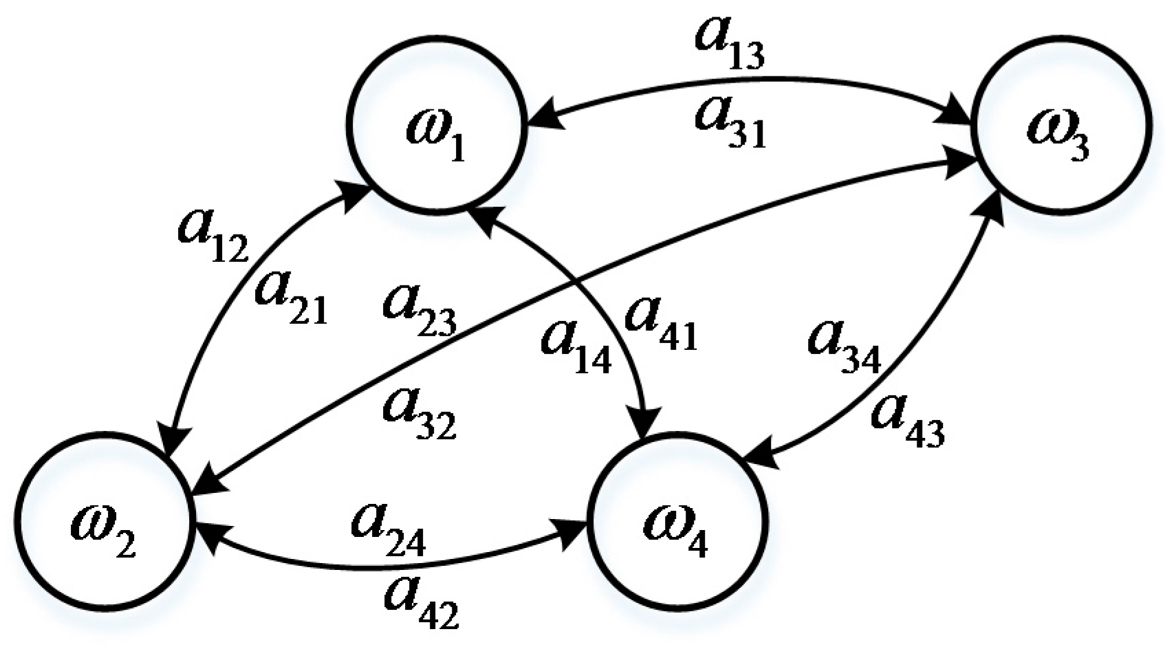
Figure 2.
Finite state machine.

Figure 3.
Overview on SOLAR gas turbine fuel system.

Figure 4.
Disturbance of ambient temperature.
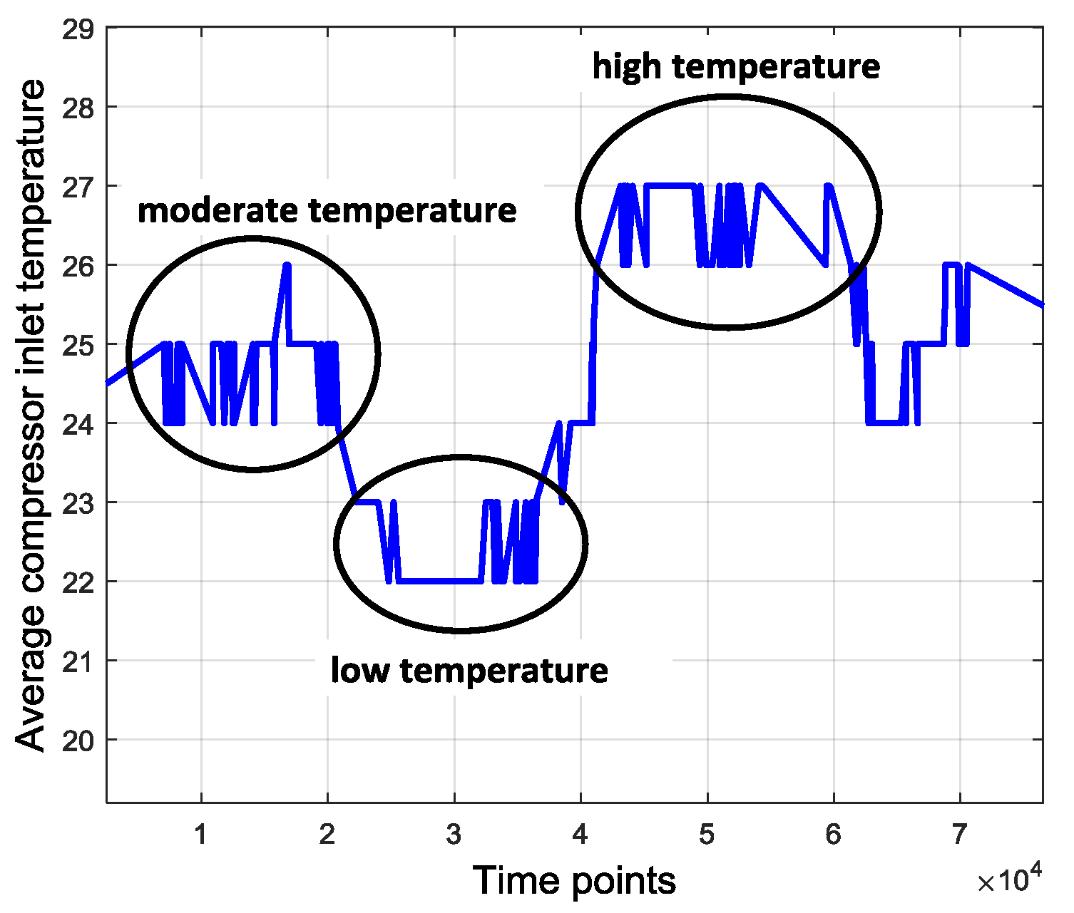
Figure 5.
Uncertainty of gas exhaust temperature.

Figure 6.
Distribution on total symbol data.
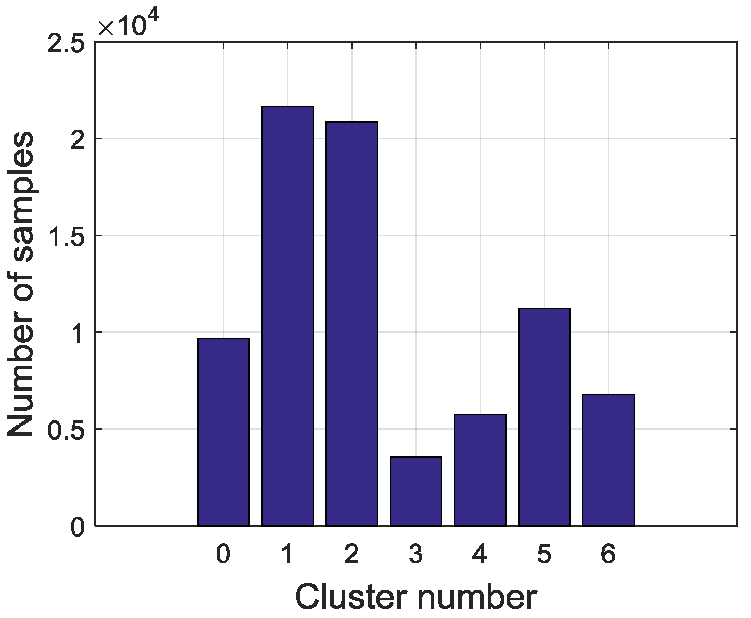
Figure 7.
Distribution of anomaly data.

Figure 8.
Time series generation with different length. Mark (+) denotes the normal series and mark (−) denotes the abnormal series.
Figure 8.
Time series generation with different length. Mark (+) denotes the normal series and mark (−) denotes the abnormal series.

Figure 9.
Schematic of FSM modeling procedures.
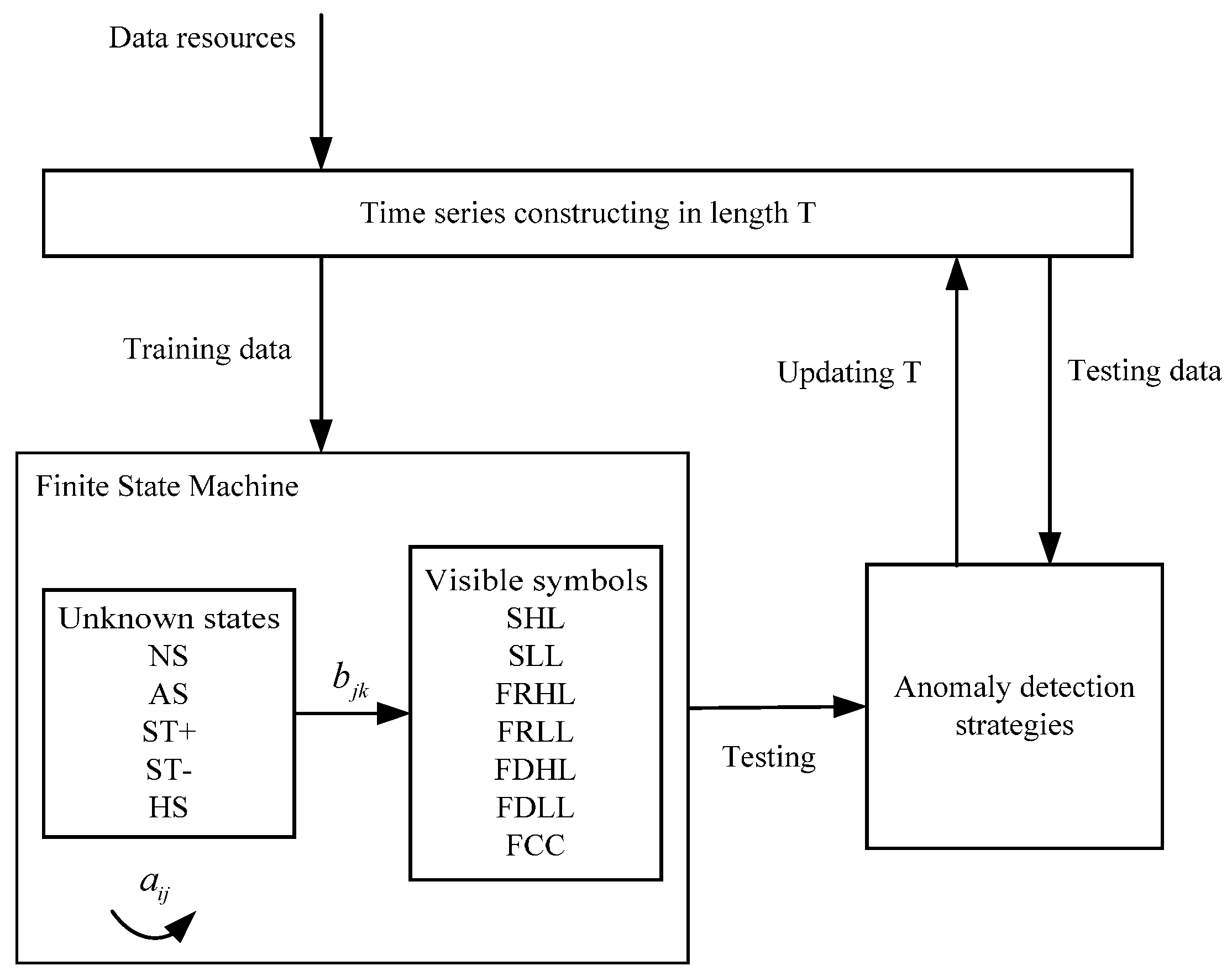
Figure 10.
Schematic of anomaly detection using the estimation strategy.
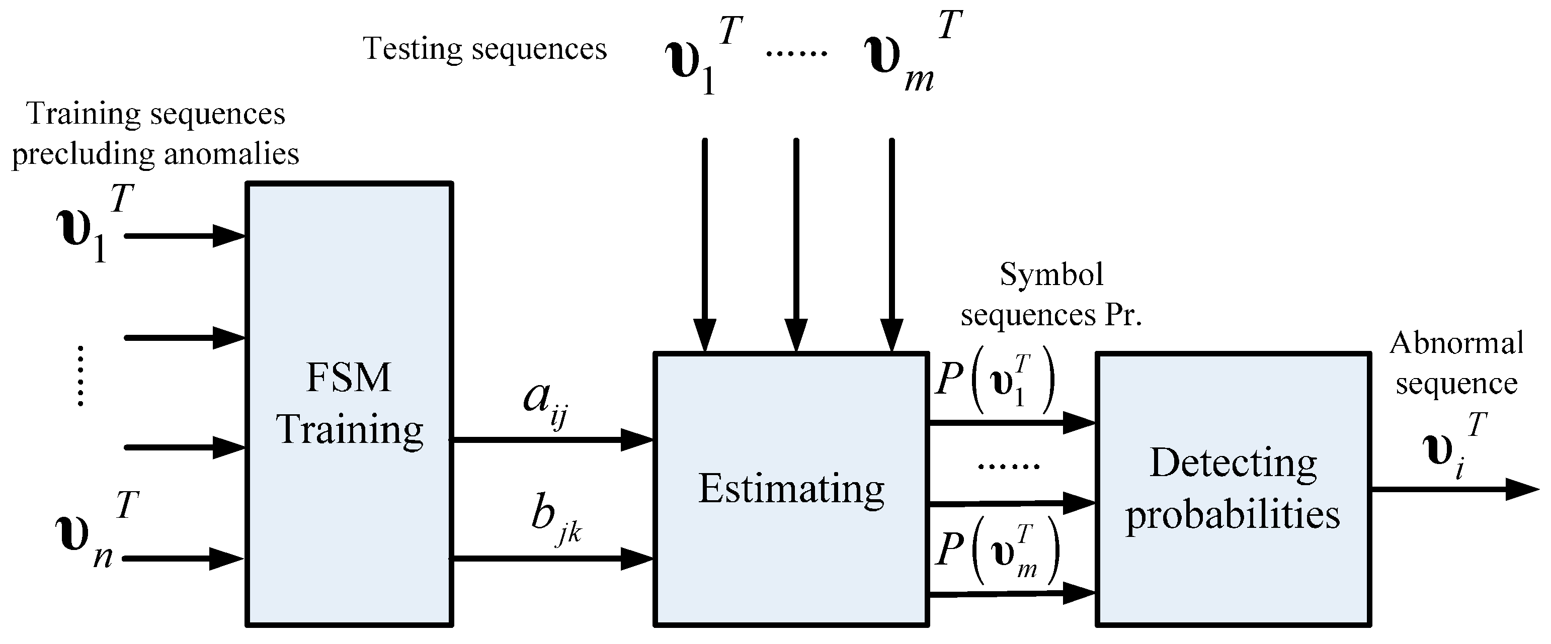
Figure 11.
Schematic of anomaly detection using the decoding strategy.

Figure 12.
Schematic diagram of Area Under ROC Curve (AUC). The surface of the area is the Receiver Operating Characteristic curve and the area of the shadow is AUC.
Figure 12.
Schematic diagram of Area Under ROC Curve (AUC). The surface of the area is the Receiver Operating Characteristic curve and the area of the shadow is AUC.

Figure 13.
An exemplary anomaly sequence.

Figure 14.
Comparison between a normal sequence and an anomaly sequence in symbolic description.

Figure 15.
ROC curve of the estimation-based model with different thresholds.

Figure 16.
Performance change with increasing threshold.

Figure 17.
Optimized thresholds for different lengths of the sequence.

Figure 18.
Comparison between the estimation-based and decoding-based models on TN rate.
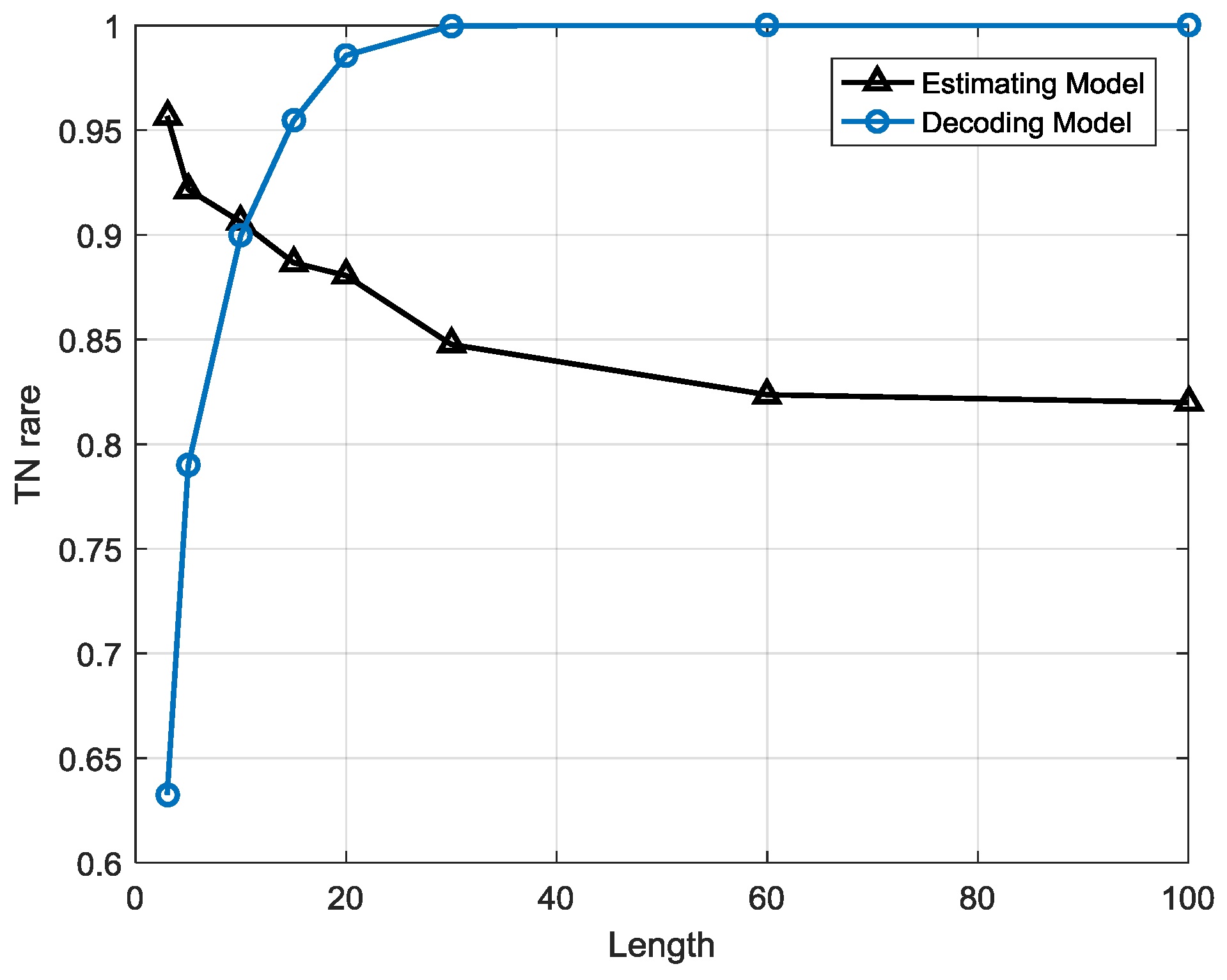
Figure 19.
Comparison between the estimation-based and decoding-based models on TP rate.
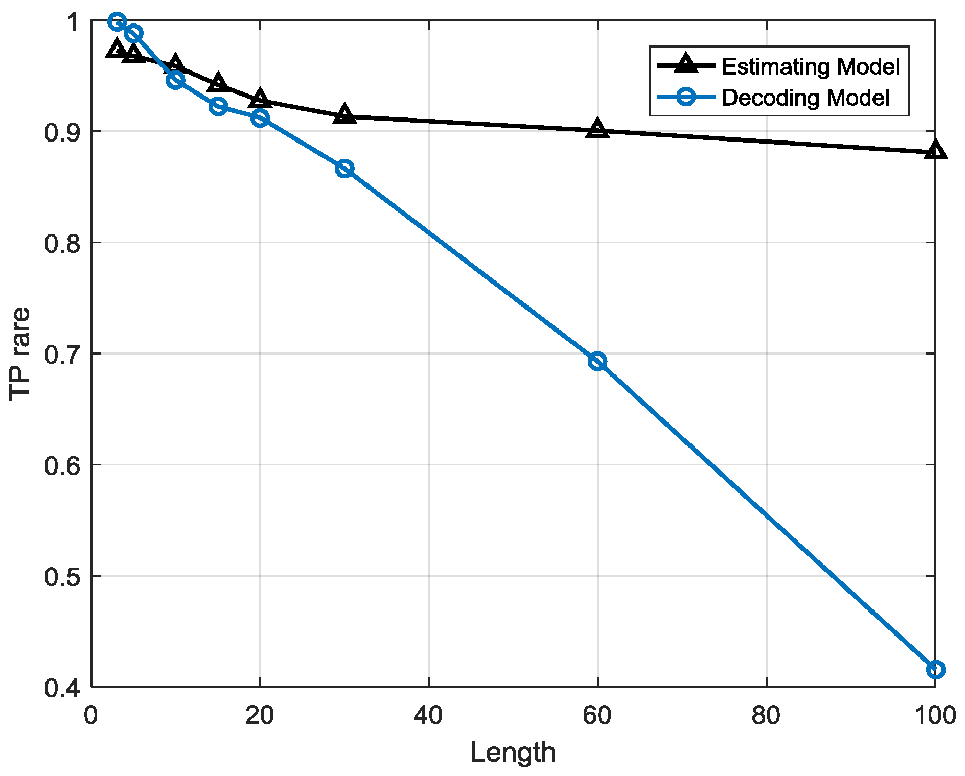
Figure 20.
Comparison between the estimation-based model and decoding-based model AUC.


Table 1.
Comparison between different current methods and ours.
| Collective Anomaly Detection | Symbolic Anomaly Detection | Our Method | |
|---|---|---|---|
| Strategy | Sequential based analysis | Symbolic and semantic based analysis | Sequential and symbolic integrated analysis |
| Advantages |
|
|
|
| Disadvantages |
|
|
Table 2.
Monitoring sensors used in symbol extraction.
| Sensor No. | Parameters | Unit |
|---|---|---|
| 92 | Average gas exhaust temperature | °C |
| 84 | Average fuel supplement temperature | °C |
| 81 | Main gas supplement pressure | kPa |
| 85 | Main gas valve demand | % |
| 98 | Average combustion inlet temperature | °C |
| 148 | Generator power | kW |
| 88 | guide vane position | % |
| 82 | Main gas nozzle pressure | kPa |
| 95 | Main gas heat value | kJ/kg |
| 96 | Main gas density | kg/m3 |
| 112 | Average compressor inlet temperature | °C |
Table 3.
Correspondence list between clusters and labels.
| Cluster No. | Label | Symbol |
|---|---|---|
| #0 | Flow rise in low load | FRLL |
| #1 | Steady in high load | SHL |
| #2 | Steady in low load | SLL |
| #3 | Fast changing condition | FCC |
| #4 | Flow rise in high load | FRHL |
| #5 | Flow drop in high load | FDHL |
| #6 | Flow drop in low load | FDLL |
Table 4.
Definition on confusion matrix.
| Actual Status | Detecting Positive | Detecting Negative |
|---|---|---|
| Positive | True Positive (TP) | False Negative (FN) |
| Negative | False Positive (FP) | True Negative (TN) |
Table 5.
Performance of the two models in each data group.
| Model | Estimation-Based Model | Decoding-Based Model | ||||
|---|---|---|---|---|---|---|
| Measurement | TP Rate | TN Rate | AUC | TP Rate | TN Rate | AUC |
| 1 | 0.9577 | 0.8977 | 0.9277 | 0.9478 | 0.9009 | 0.9244 |
| 2 | 0.9692 | 0.9052 | 0.9372 | 0.954 | 0.8938 | 0.9239 |
| 3 | 0.9549 | 0.906 | 0.9305 | 0.9393 | 0.9032 | 0.9213 |
| 4 | 0.9617 | 0.9111 | 0.9364 | 0.9336 | 0.8931 | 0.9134 |
| 5 | 0.9679 | 0.8986 | 0.9333 | 0.9334 | 0.9052 | 0.9193 |
| 6 | 0.9549 | 0.9043 | 0.9296 | 0.9567 | 0.9089 | 0.9328 |
| 7 | 0.9574 | 0.9039 | 0.9307 | 0.9445 | 0.9188 | 0.9317 |
| 8 | 0.9488 | 0.9101 | 0.9295 | 0.9444 | 0.8976 | 0.921 |
| 9 | 0.9699 | 0.908 | 0.939 | 0.9587 | 0.8861 | 0.9224 |
| 10 | 0.9442 | 0.9164 | 0.9303 | 0.9487 | 0.8905 | 0.9196 |
| Mean value | 0.9587 | 0.9061 | 0.9324 | 0.9461 | 0.8998 | 0.9229 |
Table 6.
Performance of the estimation-based model.
| Actual status | Detecting Normal | Detecting Anomaly |
|---|---|---|
| Normal | 0.9587 ± 0.0086 | 0.0413 ± 0.0086 |
| Anomaly | 0.0939 ± 0.0056 | 0.9061 ± 0.0056 |
Table 7.
Performance of the decoding-based model.
| Actual status | Detecting Normal | Detecting Anomaly |
|---|---|---|
| Normal | 0.9461 ± 0.0089 | 0.0539 ± 0.0089 |
| Anomaly | 0.1011 ± 0.0097 | 0.8989 ± 0.0097 |
Table 8.
Comparison of different models for overall accuracy.
| Models Dataset | FL | EKF | SVM | BPN | EBFSM | DBFSM |
|---|---|---|---|---|---|---|
| 1 | 0.8842 | 0.8709 | 0.9043 | 0.8823 | 0.9277 | 0.9244 |
| 2 | 0.8788 | 0.9033 | 0.8922 | 0.8945 | 0.9372 | 0.9239 |
| 3 | 0.9003 | 0.912 | 0.8933 | 0.9321 | 0.9305 | 0.9213 |
| 4 | 0.8679 | 0.8457 | 0.9208 | 0.9011 | 0.9364 | 0.9134 |
| 5 | 0.8614 | 0.8268 | 0.8822 | 0.8875 | 0.9333 | 0.9193 |
| 6 | 0.9099 | 0.8897 | 0.9012 | 0.9047 | 0.9296 | 0.9328 |
| 7 | 0.9071 | 0.8872 | 0.9188 | 0.9301 | 0.9307 | 0.9317 |
| 8 | 0.8922 | 0.9099 | 0.9189 | 0.8913 | 0.9295 | 0.921 |
| 9 | 0.8766 | 0.8962 | 0.9154 | 0.8489 | 0.939 | 0.9224 |
| 10 | 0.8999 | 0.8645 | 0.8989 | 0.8689 | 0.9303 | 0.9196 |
| Mean value | 0.8878 | 0.8806 | 0.9046 | 0.8941 | 0.9324 | 0.9229 |
© 2017 by the authors. Licensee MDPI, Basel, Switzerland. This article is an open access article distributed under the terms and conditions of the Creative Commons Attribution (CC BY) license (http://creativecommons.org/licenses/by/4.0/).
Share and Cite
MDPI and ACS Style
Li, F.; Wang, H.; Zhou, G.; Yu, D.; Li, J.; Gao, H. Anomaly Detection in Gas Turbine Fuel Systems Using a Sequential Symbolic Method. Energies 2017, 10, 724. https://doi.org/10.3390/en10050724
AMA Style
Li F, Wang H, Zhou G, Yu D, Li J, Gao H. Anomaly Detection in Gas Turbine Fuel Systems Using a Sequential Symbolic Method. Energies. 2017; 10(5):724. https://doi.org/10.3390/en10050724
Chicago/Turabian StyleLi, Fei, Hongzhi Wang, Guowen Zhou, Daren Yu, Jiangzhong Li, and Hong Gao. 2017. "Anomaly Detection in Gas Turbine Fuel Systems Using a Sequential Symbolic Method" Energies 10, no. 5: 724. https://doi.org/10.3390/en10050724
Note that from the first issue of 2016, this journal uses article numbers instead of page numbers. See further details here.