
Modeling and Validation of a Diesel Engine with Turbocharger for Hardware-in-the-Loop Applications
by
 and
and
Jinguan Yin
1, 
Tiexiong Su
1,*,
Zhuowei Guan
2,
Quanhong Chu
2,
Changjiang Meng
2,
Li Jia
2,
Jun Wang
1 and
Yangang Zhang
1 1
College of Mechatronic Engineering, North University of China, Taiyuan 030051, China
2
China North Engine Research Institute, Tianjin 300400, China
*
Author to whom correspondence should be addressed.
Energies 2017, 10(5), 685; https://doi.org/10.3390/en10050685
Submission received: 28 March 2017
/
Revised: 2 May 2017
/
Accepted: 9 May 2017
/
Published: 13 May 2017
(This article belongs to the Special Issue Internal Combustion Engines 2017)
Abstract
:This paper presents a simulator model of a diesel engine with a turbocharger for hardware-in-the-loop (HIL) applications, which is used to obtain engine performance data to study the engine performance under faulty conditions, to assist engineers in diagnosis and estimation, and to assist engineers in model-based calibration (MBC). The whole diesel engine system is divided into several functional blocks: air block, injection block, cylinder block, crankshaft block, cooling block, lubrication block, and accessory block. The diesel engine model is based on physical level, semi-physical level and mathematical level concepts, and developed by Matlab/Simulink. All the model parameters are estimated using weighted least-squares optimization and the tuning process details are presented. Since the sub-model coupling may cause errors, the validation process is then given to make the model more accurate. The results show that the tuning process is important for the functional blocks and the validation process is useful for the accuracy of the whole engine model. Subsequently, this program could be used as a plant model for MBC, to develop and test engine control units (ECUs) on HIL equipment for the purpose of improving ECU performance.
1. Introduction
Concerning the complex structure of the modern heavy duty diesel engine, the main issue in the field is how to maintain the best levels of efficiency, reliability and lifecycle cost. Diagnosis during improper operation is difficult to perform. Furthermore, testing engine control units (ECUs) directly in real engine laboratories is too expensive. Some operations and environmental limitations cannot be addressed satisfactorily in the engine laboratory, but these limitations can be overcome by diesel engine modeling simulations, which can not only estimate some hard to measure engine features, but also avoid higher experiment and time costs. In the modern process of engine control system development, the verification & validation (V-cycle) mode based on computer-aided control system design is becoming more and more important. The model-based V-cycle development mode also serves to illustrate the fact that control-oriented engine models are more essential. In this mode, hardware-in-the-loop (HIL) testing plays an important role.
A lot of engine models have been developed for different applications, and the mean value model (MVM) is widely used in the control field because of its capability of observing engine states and capturing transient responses [1]. The mean value engine model has traditionally suffered from several essential downsides which were suggested to improve the response speed of engine models [2,3,4]. Based on the basic model, some literature has combined MVM with neural networks to attain both real-time performance and high precision [5,6,7]. Since MVM is a time-domination model, ignoring the combustion process, some literature implement crank angle-based models directly into MVM to predict the engine performance [8,9,10]. There is also a lot of work implementing emission models in the form of look-up tables, algebraic polynomial expressions or neural network models into MVM to predict engine emissions [4,11,12,13,14]. Since the MVM is a model of engine air-path performance [15], some other functional blocks should be added to HIL testing.
The injection system supplying fuel to a diesel engine is considered as a controlling signal in a MVM model [16]. The injection model should have more details in a HIL testing system. In reference [17], a one-dimensional distributed model for the common rail injection system based on using basic fluid flow equations was presented. A fuel injection system driving fuel from the tank to the combustion chamber can be found in [18], and this model can be used for control applications.
The cooling system maintains the operating temperature of the engine while the coolant temperature is important to the engine and control system. Cooling systems are widely investigated by modeling and experimental tests since engine thermal management is an important way to reduce engine fuel consumption and to increase efficiency [19,20,21,22,23]. Some cooling systems use mechanical pumps which are modeled by dynamic thermal modeling or hydraulic circuits [24,25]. Another cooling system equipped with an electric pump can also be found in [23,26]. The lubrication system provides a protective layer to prevent metal to metal contact, especially between piston rings and cylinder walls. Some literature focuses on the distribution of flow and pressure of the lubrication system [27,28].
The MVM models presented by the above literature focus mostly on the air system features. Concerning the absence of the complete engine operations, the extension of the model is necessary to simulate the start-run-stop operation conditions, which makes it possible to apply it in HIL and fault diagnosis. Because of the nonlinear nature of diesel engines equipped with turbochargers, the linear interpolation method for parameters is not satisfactory. Sub-model coupling may cause errors, so the tuning and validation processes are important for the accuracy of MVM.
For the purpose of HIL testing and diagnosis, this paper proposes a diesel engine model with several functional blocks: air, injection, cylinder, cooling, lubrication, and accessories. The diesel model is an extended MVM model, while at the same time it is also a block oriented model with low computational burden and required accuracy. The diesel model is implemented based on Matlab/Simulink. The parameters of every sub-model are tuned using a set of experimental data, and the tuning process and its results are shown in detail. After that, the whole model is validated using another set of experimental data. It shows that the dependence on maps can be reduced by using parameterized functions to describe the diesel engine model using linear or nonlinear least-squares optimization as the tuning method for every sub-model parameter estimation. It is shown that the initialization method is important for the parameter estimation, and it can reduce errors by using both the sub-models and whole model in the optimization. The diesel engine simulator model can be used in control system development and HIL applications.
2. Diesel Engine Modeling
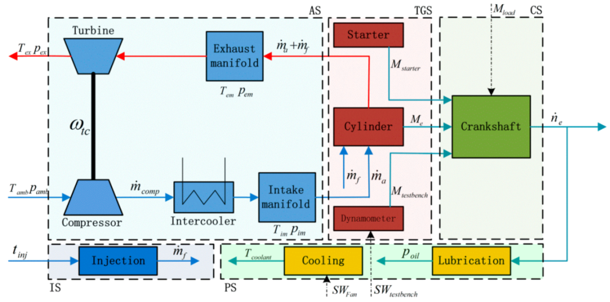
In this part, the concept of our diesel engine model is described. It simulates the performance of a 15.8 L electronic unit pump (EUP) diesel engine equipped with a turbocharger. The basic diesel engine characteristics are summarized in Table 1. For the purpose of HIL testing and control strategy development, the diesel engine model is divided into several blocks. The model architecture, as shown in Figure 1, consists of some systems and every system has one or more blocks.
The air system (AS) contains the air block which has nonlinear and dynamic behavior. The jnjection system (IS) contains the injection block. It has a faster dynamic behavior than other systems and it is a unit injector in this paper. The torque generation system (TGS) contains the cylinder block and accessory block. The combustion process takes place in the cylinder and generates torque, heat and emissions. This paper concerns the torque, so the cylinder block is in the TGS. The accessory block contains the starter and dynamometer. Since the starter generates torque and transmits it to the crankshaft when the engine started and the dynamometer also generates torque on the test bench, the accessory block is in the TGS. The crankshaft system (CS) contains the crankshaft block. The protection system (PS) contains the cooling block and lubrication block since they protect the engine from overheating and wear, respectively.
2.1. Air System
The AS comprises the air block and it is a MVM model. We use dynamic differential equations to describe the air block and it has five sub-models in this paper: turbocharger, intercooler, intake manifold, air mass into cylinder and exhaust manifold. Detailed descriptions of these submodels are given in the following sections.
2.1.1. Turbocharger
The turbocharger model consists of a turbine, compressor and turbocharger rotor which transfer powers from the turbine to the compressor. The turbocharger can be modeled by isentropic thermal efficiency. The output temperature of compressor is given by:
The compressor power can be modeled using the following equation:
where the inlet temperature of compressor is equal to the ambient air temperature . is the ambient air pressure, is the outlet pressure of compressor, is specific heat ratio of air, is the air specific heat in constant pressure, is the compressor efficiency and is the mass flow through the compressor. is modeled as follows [16]:
where is the corrected mass flow is defined as , and corrected speed is defined as . and are reference temperature and pressure respectively. is the pressure ratio over the compressor. is the radius of compressor, is the turbocharger rotor rotation speed, is the blade tip speed. and are tuning parameters.
represents the maximum corrected air mass flow through the compressor and is a factor for the maximum pressure ratio over the compressor.
is modeled as follows:
where the tuning parameters are , , , , and . represents the maximum compressor efficiency.
represents the optimum value of corrected mass flow. represents the optimum value of pressure ratio for the maximum compressor efficiency.
The turbine power is modeled as follows:
In which is the turbine generated power, is the inlet temperature of turbine, and are the inlet and outlet pressure of turbine respectively, is the exhaust specific heat in constant pressure, is the turbine efficiency which is modeled using a 2-D lookup table based on engine speed and exhaust mass flow, and is the mass flow though the turbine which is simplify modeled as follows:
Compressor connects to turbine with turbocharger rotor, and its dynamic model is:
where is the rotor speed, and is the turbocharger inertia.
2.1.2. Intercooler
The temperature and pressure of fresh air become higher after compression by the compressor. Supposing that the intercooler inlet temperature is equal to the outlet temperature of the compressor and the intercooler outlet temperature is equal to the temperature of the intake manifold, the intercooler can be modeled using the heat exchanger efficiency as:
in which is the temperature of intake manifold, is the temperature of coolant, and is the intercooler efficiency. The pressure drop in the intercooler is so small that this paper supposes the intercooler inlet pressure is equal to outlet pressure.
2.1.3. Manifold
The intake and exhaust manifold have the same modeling assumption and method, so only the intake manifold is discusssed here. Neglecting the effects of heat transfer in the intake manifold and assuming the mass flow in the intake manifold is kept constant, the temperature of the intake manifold is not changed. According to the first law of thermodynamics and the ideal gas law, the pressure of the intake manifold can be modeled as follows:
where is the intake manifold volume, is the air mass flow into the cylinder, and ideal gas constant.
2.1.4. Air Mass into the Cylinder
The air mass flow into cylinder can be modeled using volumetric efficiency, given by:
in which is the engine displacement volume, is the engine speed, and is the volumetric efficiency which is a tuning parameter that can be modeled as follows:
2.2. Injection System
In this paper, the fuel-injection system is an electronic unit pump system. The fuel flow into the cylinder is controlled by an electrically controlled valve. The amount of fuel metered by the injection valve is proportional to the square root of the pressure over the valve and the opening time. The fuel injector is opened once each cycle, so the fuel delivery per cycle per cylinder can be modeled as follows:
In which is a tuning parameter including the influence of pressure and other factors, is the injection duration, is depended by the opening and closing times of the injector valve.
The fuel mass flow is given by:
In which is the number of cylinders.
2.3. Torque Generate System
In this paper, the TGS contains the cylinder block and accessory block since both of them generate torque. As an expansion, the TGS can contain more blocks such as a motor for a hybrid vehicle.
2.3.1. Cylinders
This paper mostly pays attention to the torque which generated in the cylinders. The effective torque of a diesel engine is modeled by three parts: the gross indicated torque per cycle, the pumping torque from the difference between the intake and exhaust manifold pressure, and the friction torque consumed by the engine components and auxiliary devices. It can be expressed as:
where is the engine effective torque, is the gross indicated torque, is the pumping torque, and is the friction torque.
The gross indicated torque is modeled by the amount of fuel injected into cylinders per cycle as follows:
In which is the heating value of fuel, is the number of crank revolutions in a complete cycle, and is the indicated efficiency modeled as:
In which is the compression ratio. is the gas specific heat capacity ratio in the cylinder. The tuning parameter represents the combustion chamber efficiency.
The pumping torque is modeled as:
The friction torque is assumed to be a quadratic polynomial depended on engine speed:
The tuning parameters , and are fitting coefficients.
2.3.2. Accessory
The accessory block is divided into the starter and dynamometer. For the purpose of HIL testing, the working principles of the starter and dynamometer are ignored. What this paper is concerned with is the torque which the black-box models generate. The starter model simulates the torque change of the starter motor in the engine starting process. Assuming that the starter torque decreases linearly as the engine speed increases, starter torque will be zero when the engine speed reaches the speed at which the injector starts working. It can be shown as:
The dynamometer model simulates the engine bench test, and there are two modes in this paper. One is speed control mode and the other is torque control mode. The dynamometer model is controlled by a switch key. In the speed control mode, a PID controller which as a triggered system will work if it is switched on and the engine speed is greater than the target speed, or the dynamometer exports zero torque. In the torque control mode, the dynamometer model exports the target torque:
In which is the switch signal, is the target torque in the torque control mode, is the target speed in the speed mode, is the error given by .
2.4. Crankshaft System
The crankshaft system contains the crankshaft block. The rotation speed of the engine is calculated using Newton’s second law as follows:
In which is the inertia of crankshaft.
2.5. Protection System
The PS contains the cooling block and lubrication block. A lot of research has been done in this field, and they take the flow rate in the cooling and lubrication circuit into account. What we are concerned with is the coolant temperature and oil pressure in the HIL testing system, for which a simple but effective model is given below.
2.5.1. Cooling Block
The mean effect of the cooling system is considered only for the mean value model. Supposing there is no thermal exchange between full circulation and simple circulation, all friction torque transforms into heat, and the most of heat from combustion is carried off by the cooling system. The cooing block is modeled using Newton’s cooling law, which is given by:
In which is the coolant temperature, is the thermostat start temperature, is the heat released to the environment from engine, is heat released to the full circulating, is thermal capacity, , is the heat transfer coefficient by using air cooling, is the heat transfer coefficient by using compulsory fan-cooling, and is the heat transfer coefficient using full circulating cooling.
2.5.2. Lubrication Block
The engine should be protected when the lubrication oil pressure is too low. It is important to have a lubrication oil pressure model for the HIL testing and diagnosis application. For the mean value model, the lubrication oil pressure is considered while the oil temperature is neglected. It supposes that the oil pressure is well-distributed in the lubrication system. The lubrication oil pressure is modeled as:
where is the lubrication oil pressure, tuning parameters , and are fitting coefficients.
3. Model Tuning and Validating
3.1. Tuning
As described in Section 2, the diesel engine model in this paper utilizes lots of assumptions about the engine physical process. Many error sources such as experimental errors, modeling errors, etc would lead to engine model inaccuracy. In order to tune and validate the engine model, stationary measurements which cover a wide range of engine operating conditions are performed in the engine laboratory. In the experiment, engine speeds of 1000, 1100, 1300, 1400, 1500, 1700, 1900 and 2100 rpm have been chosen for the tuning process, and the engine load ranges from 10% to 100% with a 10% interval. The measured variables can be found in Table 2.
In this paper, relative error is used to evaluate the tuning and the validation of the model, and the relative error between measured variable and modeled variable is calculated as follows:
Firstly the injection model is tuned. Equation (15) can be rewritten as:
The tuning parameters are and . Using linear least-squares method to minimize with and as the optimization variables, is the model and is calculated from stationary measurements which are used as the input of Equation (28) during the tuning process.
The tuning result in Figure 2 shows that the injection model has a maximum relative error of 8.02% and a mean relative error of 2.93%. We note that the units of in Equation (28) are rpm, but in Figure 2 it is rps.
Then the air mass into cylinder model is tuned. Substituting Equation (14) into Equation (13) we can rewrite it as follows:
The tuning parameters are , , and . The purpose is to minimize in the air mass into the cylinder model. It can be replaced by minimizing . Using a linear least-squares method to minimize it with , , and as the optimization variables. is the model and is calculated from stationary measurements which are used as the input of Equation (29) during the tuning process. The tuning result is shown in Figure 3.
In Figure 3, Figure 3a shows that the measurements of volumetric efficiency are nonlinear and the error between the model of volumetric efficiency and the measurements is large in some regions. Since the volumetric efficiency model as a sub-model of the air mass into the cylinder model, and the tuning purpose is to minimize , Figure 3c shows that tuning result is good and the model has a max. relative error of 6.4% and a mean relative error of 1.34%. After that, Equation (11) can be rewritten as:
In the experiment, engine operations are determined by the engine speed and load. The coolant temperature, the intercooler inlet and the outlet temperature are measured in every operation, so the intercooler efficiency can be modeled as a 2-D lookup table based on engine speed and load. The result is shown in Figure 4.
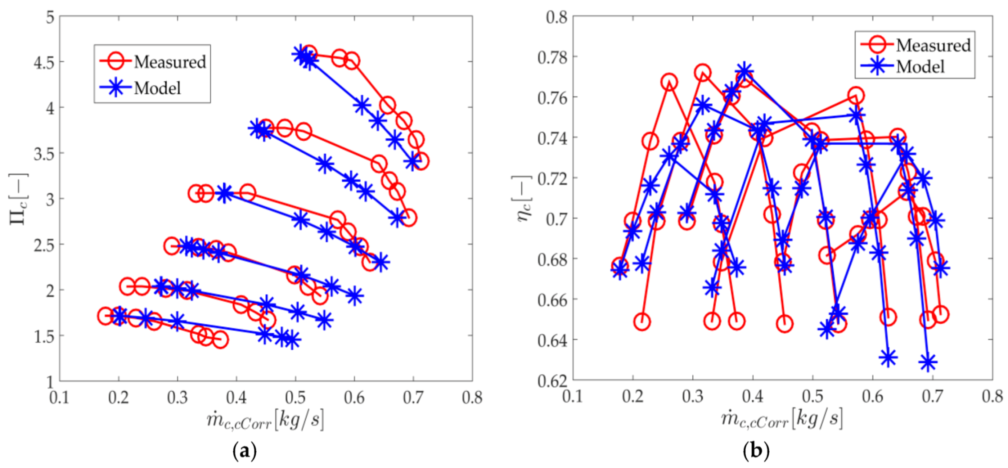
Then the turbocharger model should be tuned. In the compressor model, there are two sub-models having parameters: model and model. The corrected speed and corrected mass flow are used in the compressor map. A series of steady state measurement points are present based on them and is given for each point. Substituting Equation (5) into Equation (4), the tuning parameters are and . The purpose is to minimize in the compressor mass flow model. Using nonlinear least-squares method to minimize it with , and as the optimization variables. is the model and is calculated according to stationary measurements which are used as the input during the tuning process. The initializing values should be given to the tuning function for nonlinear parameter estimation. The tuning would be disappointing if the initializing values aren't reasonable. In this part, the initialization values are defined as follows:
should be estimated firstly and the tuning result is shown in Figure 5a. The result shows that the model fits the measurements except for when the rotor speed is too high. The model has a max. relative error of 17.4% and a mean relative error of 8.5%.
For the compressor efficiency model, the purpose is to minimize . Using the nonlinear least-squares method to minimize it with , , , , and as the optimization variables. is the model as shown in Equations (6) and (7) and is calculated from stationary measurements as follows:
The start values are defined as:
The tuning result is shown in Figure 5b. The result shows that the compressor efficiency model has a max. relative error of 5.18% and a mean relative error of 1.65%.
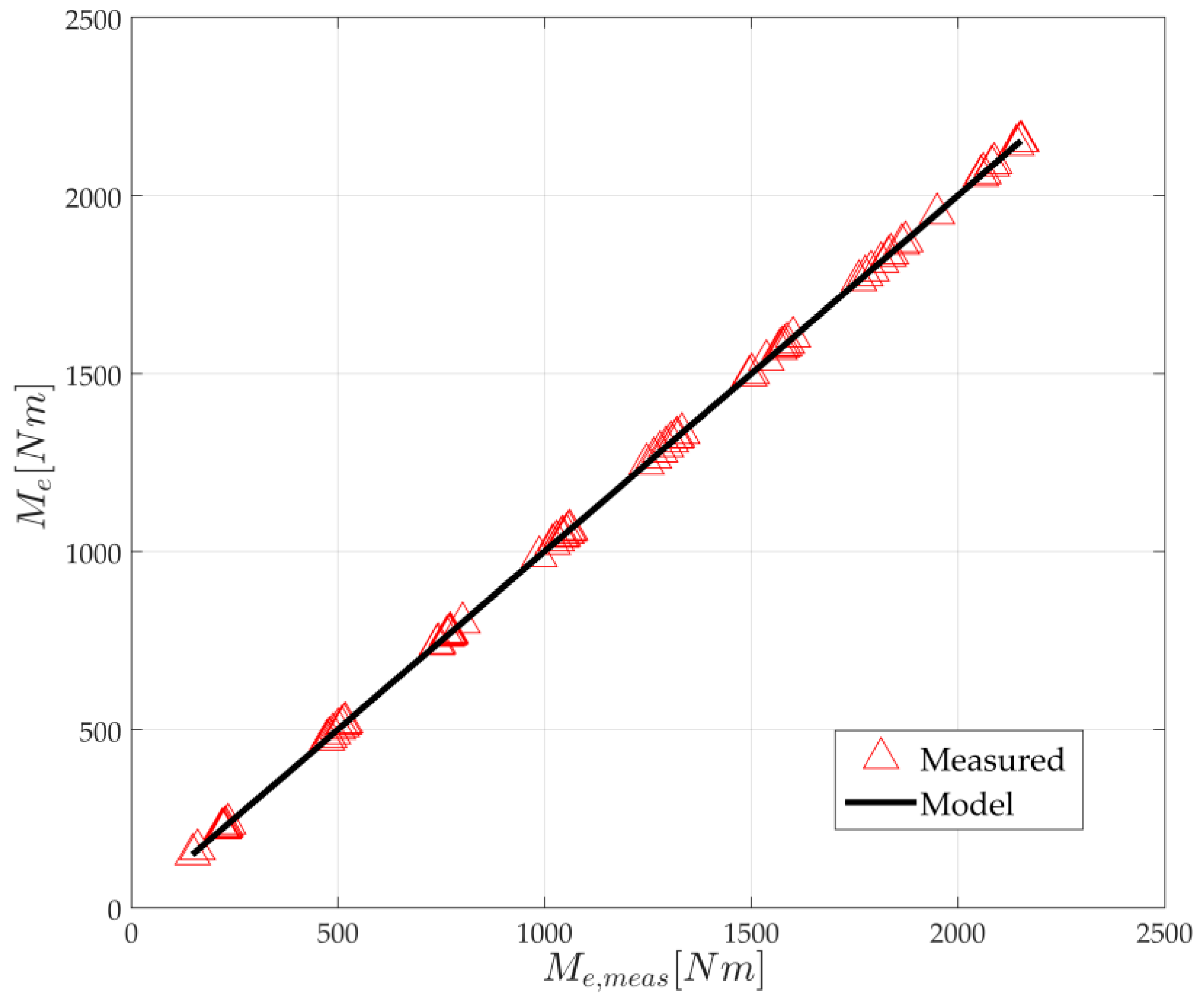
For the cylinder model, and can be calculated by measurements, and the tuning parameters are , , , . Substituting Equations (18)–(21) into Equation (17) it can be rewritten as:
So the purpose is to minimize in the torque generation model. Using the linear least-squares method to minimizes it with , , and as the optimization variables. is the model and is calculated from stationary measurements which are used as the input of Equation (34) during the tuning process. The tuning result in Figure 6 shows that the relative error is nearly zero.
For the lubrication system, , and are tuning parameters and the measurements are oil pressure, coolant temperature and engine speed. Using the linear least-squares method to minimize with the tuning parameters as the optimization variables, the tuning result is shown in Figure 7, which shows that the lubrication oil pressure model has a max. relative error of 8.32% and a mean relative error of 3.26%.
3.2. Validation
After the tuning process, the validation is perfored. The validation measurements are done under six operating conditions with a 1200/1600/1800 rpm engine speed and a 30%/60% load for every value of engine speed. All the parameters are tuned using a Matlab (2015B, MathWorks, Natick, MA, USA) script and the validation process is implemented in Simulink. During the validation, the diesel engine submodels should be validated one by one considering the model coupling. For example, the boundary inputs are given out for the model and the intercooler is the first validated submodel, while the output of the intercooler model is compared with the validation measurement. The next submodel would be validated if the result is suitable, otherwise the parameters of the intercooler model should be adjusted. Then the submodel output should be the input of next submodel instead of the validation measurement. Finally the whole model is run and every submodel output is validated. Some parameters should be adjusted if the error is too large.
Firstly the injector model is validated, the boundary inputs are engine speed and injection duration which are the measurement data from the validation measurement. The result is shown in Figure 8, which has a maximum error of 1.12%. The accuracy is acceptable and the next submodel can be validated, otherwise the injector model should be checked and validated again.
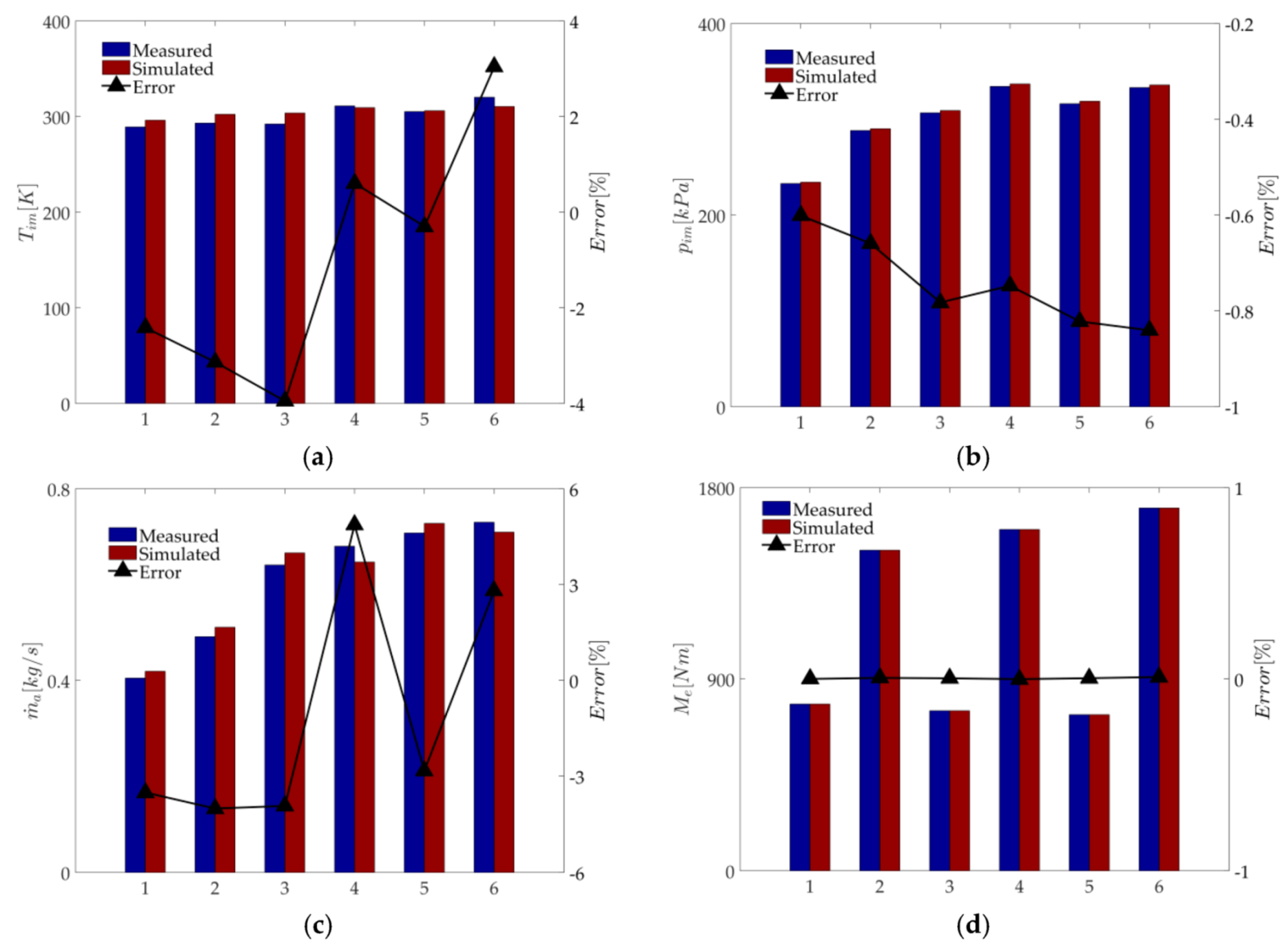
Then the intercooler model is validated, the boundary inputs are compressor outlet temperature and coolant temperature which are measurement data from the validation measurement. The validation result is shown in Figure 9a. The maximum error in the validation is 3.95%. Since the intercooler efficiency is modeled as a 2-D lookup table, it is suggested that there are enough breakpoints to develop the model. If the accuracy of the intercooler model is acceptable, the intake manifold model can be connected with the validated intercooler model. The output of the intercooler model has to be the input of the intake manifold model instead of the measurement data (). The air mass of the intake manifold inlet and outlet data are taken from the validation measurements. The validation result is shown in Figure 9b. The maximum error in the validation is 0.93%. In a similar way, the exhaust manifold can be validated which does not need to be discussed here. It seems the result is good enough, but considering an input of the model is the air mass into cylinder which is calculated from the intake manifold pressure, a decoupling process should be implemented, otherwise the model error will be very large. The input of the air mass into cylinder model are the engine speed from the validation measurements, intake manifold pressure from the intake manifold model, and intake manifold temperature from the intercooler model. As shown in Figure 9c, the maximum error in this model validation is 4.86%. After this step, the intake manifold and air mass into cylinder model are coupled and simulated. is corrected in this step to acquire a higher accuracy model. Then the cylinder model is connected with the intake/exhaust manifold model and injection model. Using these model outputs as the inputs of the cylinder model, the validation process is implemented. Since the intake/exhaust manifold model are corrected, the simulation result of the cylinder model is satisfactory, which is shown in Figure 9d.
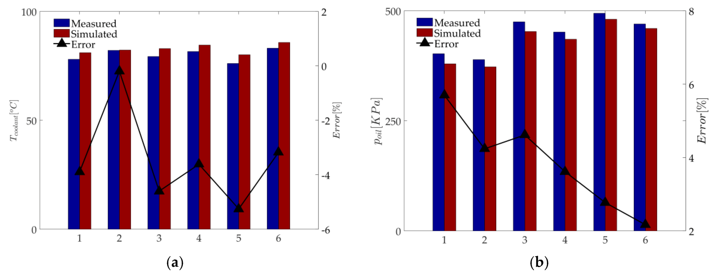
After that, the protection system is connected to the engine model and validated. The coolant temperature has an influence on the intercooler model and lubrication model, so it is important to make sure that the coolant model is accurate enough. In this step, the coolant temperature is validated firstly, followed by the lubrication model. As shown in Figure 10, the maximum errors of the coolant temperature and oil pressure are 5.26% and 5.69%, respectively.
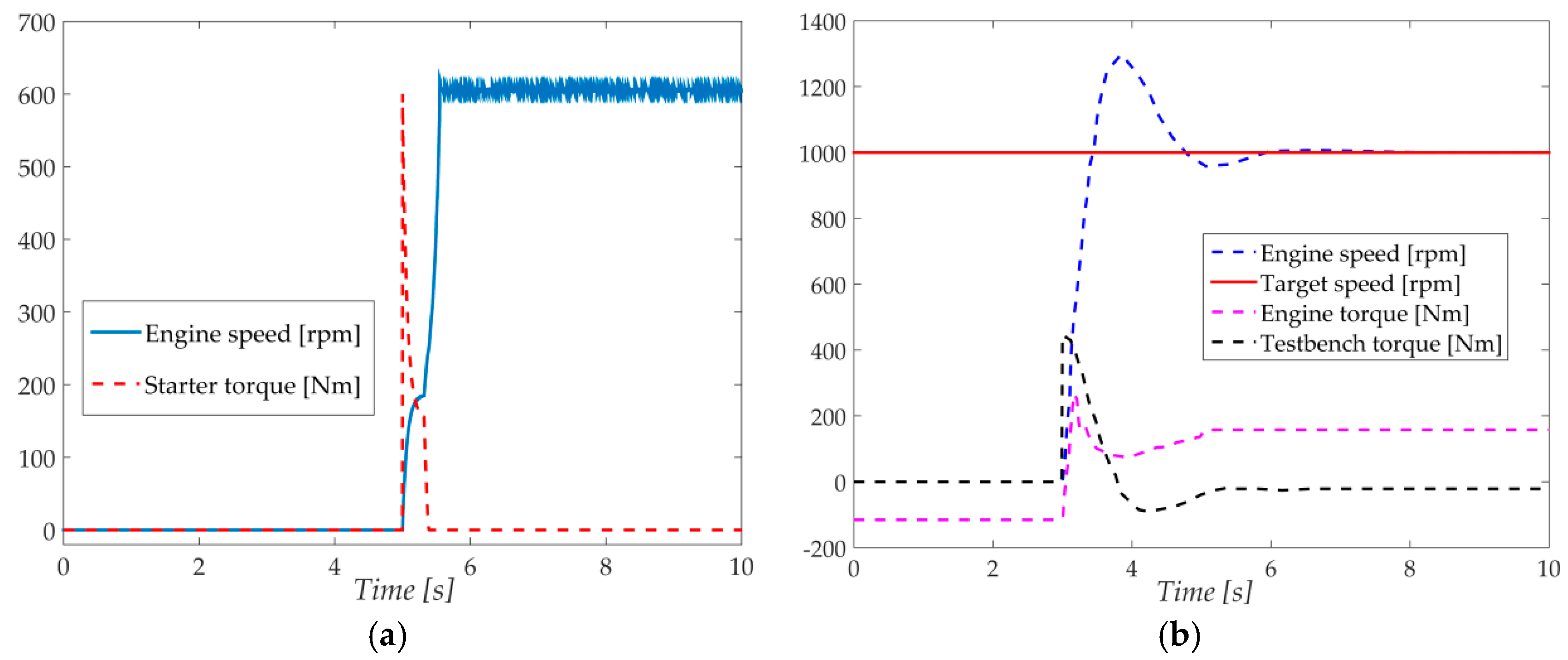
Then the accessory model in TGS is validated. In this part, the model is implemented in a black-box way instead of using a physics principle which is rather complicated to describe. The starter drags the engine to rotate when the starting switch is on, and it stops when the engine speed is 200 rpm. After that, the injection system starts working and the engine accesses its idling operating conditions if there isn’t any acceleration signal. The simulation result is shown in Figure 11a. At 5 s, the starting switch is on and the starter works. The starter torque is 600 Nm at first, then it linearly decreases and injector starts working at 200 rpm engine speed. After this, the starter is off and the starter torque becomes zero again. When the engine test bench switch is on, engine starts running under the test conditions. After 3 s, the engine test bench switch is on and the target engine speed is 1000 rpm. As shown in Figure 11b, the test bench drags the engine to run to the target speed. The engine speed, engine torque, and test bench torque would become stable after the engine speed reached the target speed. The change of engine speed has a certain lag behind the test bench torque.
Finally, the turbocharger model is connected to the engine model and validated. The boundary inputs are ambient pressure, ambient temperature and compressor outlet pressure which is connected to the intercooler model. Since the intercooler model only considers the temperature drop, the compressor outlet pressure is equal to the intake manifold pressure and the compressor outlet temperature is connected to the intercooler inlet temperature. The inputs of the turbine are the mass flow though the turbine and the pressure before and after the turbine. Because of the input of the compressor model is from the engine model, the error of the compressor flow model is large, and the turbine efficiency is modeled by a lookup table based on the engine speed, would have a big error due to the coupling of turbocharger and engine. An obvious effect is the error of intake manifold pressure which would become very large, so it's important to validate it and to adjust the turbine efficiency table to reduce the error. The result shows that the turbine efficiency accuracy has a great influence on the engine model. What we should do in this step is to adjust the turbine efficiency map to keep the errors of the intake manifold pressure model on a reasonable level.
4. Conclusions
A simulator of a diesel engine model with a turbocharger is developed for HIL applications. For the purpose of simulating the actual working condition and some fault conditions, the standard MVM model is extended. The air system model is a standard MVM model. The injection system is an electronic unit injector modeled based on the injector features. Since the engine starting process is complex and it lasts for a rather short period, it is difficult to model this process, so a linear model for the starter is given. The dynamometer is modeled based on its work principle instead of the physical process. The focus of the cylinder model is torque generation, which is also a MVM model. A simple but effective model of the protection system is also given out.
In order to improve the accuracy of this diesel model, tuning and validations processes are carried out. The parameters of the diesel model are determined successfully in the tuning process and are adjusted in the validation process to improve the accuracy of the model. The results show that the parameter recognition results are rather good, but with regard to the whole model, there is a relatively large error due to the coupling effect of the sub-models, therefore the model validation and the parameter adjustment are necessary, which are mainly about the coupling between the turbocharger model and the engine model, and the coupling between the intake manifold model and the air mass into cylinder model. Both influence the pressure of the intake manifold greatly. In addition, the precision of the coolant temperature in the cooler model would have a huge effect on the intercooler model and the engine oil pressure model. Finally the whole model simulation result has a 6% error compared to the experimental data. This engine model simulator can be further used in the fields of ECU development, HIL application and MBC design.
Acknowledgments
The authors gratefully acknowledge the financial support by the National Natural Science Foundation of China under Grant No. 51605447.
Author Contributions
Changjiang Meng, Quanhong Chu and Jinguan Yin designed and performed the experiments; Jinguan Yin designed the model; Li Jia contributed analysis tools and HIL equipment; Jinguan Yin, Zhuowei Guan, Jun Wang and Yangang Zhang analyzed the data; Jinguan Yin and Tiexiong Su contributed to the editing and reviewing of the document.
Conflicts of Interest
The authors declare no conflict of interest.
References
- Cong, G.; Gerasimos, T.; Peilin, Z.; Hui, C. Computational investigation of a large containership propulsion engine operation at slow steaming conditions. Appl. Energy 2014, 130, 370–383. [Google Scholar]
- Jensen, J.P.; Kristensen, A.F.; Serensen, S.C.; Houback, N.; Hendricks, N. Mean Value Modeling of a Small Turbocharged Diesel Engine; Society of Automotive Engineers (SAE) Technical Paper: 910070; SAE: Warrendale, PA, USA, 1991. [Google Scholar]
- Moskwa, J.J.; Hendricks, J.K. Modeling and validation of automotive engines for control algorithm development. Trans. ASME J. Dyn. Syst. Meas. Control 1992, 114, 278–285. [Google Scholar] [CrossRef]
- Guzzella, L.; Onder, C.H. Introduction to Modeling and Control of Internal Combustion Engine Systems, 2rd ed.; Springer: Berlin/Heidelberg, Germany, 2010. [Google Scholar]
- Amir-Mohammad, S.; Amir, H.S. A new approach in improvement of mean value models for spark ignition engines using neural networks. Expert Syst. Appl. 2015, 42, 5192–5218. [Google Scholar]
- Janakiraman, V.M.; Nguyen, X.; Assanis, D. Nonlinear identification of a gasoline HCCI engine using neural networks coupled with principal component analysis. Appl. Soft Comput. 2013, 13, 2375–2389. [Google Scholar] [CrossRef]
- Cay, Y.; Cicek, A.; Kara, F.; Sagiroglu, S. Prediction of engine performance for an alternative fuel using artificial neural network. Appl. Therm. Eng. 2012, 37, 217–225. [Google Scholar] [CrossRef]
- Ruixue, L.; Ying, H.; Gang, L.; He, S. Control-oriented modeling and analysis for turbocharged diesel engine system. Adv. Mech. Eng. 2013, 2, 855–860. [Google Scholar]
- Paolo, C.; Agostino, G.; Nicola, P.; Ugo, C.; Enrico, L.; Annachiara, P. Development and Validation of a “Crank-angle” Model of an Automotive Turbocharged Engine for HiL Applications. Energy Procedia 2014, 45, 839–848. [Google Scholar]
- Fadila, M.; Charbel, S. Combined mean value engine model and crank angle resolved in-cylinder modeling with NOx emissions model for real-time Diesel engine simulations at high engine speed. Energy 2015, 88, 515–527. [Google Scholar]
- Giakoumis, E.G.; Alafouzos, A.I. Study of diesel engine performance and emissions during a Transient Cycle applying an engine mapping-based methodology. Appl. Energy 2010, 87, 1358–1365. [Google Scholar] [CrossRef]
- Benz, M.; Onder, C.H.; Guzzella, L. Engine emission modeling using a mixed physics and regression approach. J. Eng. Gas Turbines Power 2010, 132, 042803. [Google Scholar] [CrossRef]
- Kolmanovsky, I.V.; Stefanopoulou, A.G.; Moraal, P.E.; van Nieuwstadt, M. Issues in modeling and control of intake flow in variable geometry turbocharged engines. In Proceedings of the 18th IFIP Conference on System Modelling and Optimization, Detroit, MI, USA, 22–25 July 1997; Volume 396, pp. 436–445. [Google Scholar]
- Kamyar, N.; Amir, H.S. An extended mean value model (EMVM) for control-oriented modeling of diesel engines transient performance and emissions. Fuel 2015, 154, 275–292. [Google Scholar]
- Paul, D.; Dariusz, C.; Keith, G.; Nick, C.; Yukio, Y.; Yusuke, Y.; Toru, H. On-Engine Validation of Mean Value Models for IC Engine Air-Path Control and Evaluation. IFAC Proc. Vol. 2014, 47, 2987–2993. [Google Scholar]
- Wahlstrom, J.; Eriksson, L. Modelling diesel engines with a variable-geometry turbocharger and exhaust gas recirculation by optimization of model parameters for capturing non-linear system dynamics. Proc. Inst. Mech. Eng. Part D J. Automob. Eng. 2011, 225, 960–986. [Google Scholar] [CrossRef]
- Gupta, V.K.; Zhang, Z.; Sun, Z. Modeling and control of a novel pressure regulation mechanism for common rail fuel injection systems. Appl. Math. Model. 2011, 35, 3473–3483. [Google Scholar] [CrossRef]
- Lino, P.; Maione, B.; Rizzo, A. Nonlinear modelling and control of a common rail injection system for diesel engines. Appl. Math. Model. 2007, 31, 1770–1784. [Google Scholar] [CrossRef]
- Buono, D.; Senatore, A.; Prati, M.V.; Manganelli, M. Analysis of the Cooling Plant of a High Performance Motorbike Engine; Society of Automotive Engineers (SAE) Technical Papers: 2012-01-0354; SAE: Warrendale, PA, USA, 2012. [Google Scholar]
- Piccione, R.; Bova, S. Engine Rapid Shutdown: Experimental Investigation on the Cooling System Transient Response. J. Eng. Gas Turbines Power 2010, 132, 072801. [Google Scholar] [CrossRef]
- Algieri, A.; Amelio, M.; Bova, S.; Morrone, P. Energy Efficiency Analysis of Monolith and Pellet Emission Control Systems in Unidirectional and Reverse-Flow Designs. SAE Int. J. Engines 2010, 2, 684–693. [Google Scholar] [CrossRef]
- Piccione, R.; Vulcano, A.; Bova, S. A Convective Mass Transfer Model for Predicting Vapor Formation within the Cooling System of an Internal Combustion Engine after Shutdown. J. Eng. Gas Turbines Power 2010, 132, 022804. [Google Scholar] [CrossRef]
- Teresa, C.; Sergio, B.; Mario, B. A Model Predictive Controller for the Cooling System of Internal Combustion Engines. Energy Procedia 2016, 101, 582–589. [Google Scholar]
- Pizzonia, F.; Castiglione, T.; Bova, S. A Robust Model Predictive Control for Efficient thermal management of Internal Combustion Engines. Appl. Energy 2016, 169, 555–566. [Google Scholar] [CrossRef]
- Castiglione, T.; Pizzonia, F.; Bova, S. A Novel Cooling System Control Strategy for Internal Combustion Engines. SAE Int. J. Engines 2016, 9, 294–302. [Google Scholar] [CrossRef]
- Mohammad, H.S.; Thomas, H.M.; John, R.W.; Darren, M.D. A Smart Multiple-Loop Automotive Cooling System—Model, Control, and Experimental Study. IEEE/ASME Trans. Mechatron. 2010, 15, 117–124. [Google Scholar]
- Chun, S.M. Network analysis of an engine lubrication system. Tribol. Int. 2003, 36, 609–617. [Google Scholar] [CrossRef]
- Hassan, M.N.; Rafic, Y.; Hassan, S.; Mustapha, O. Modeling with Fault Integration of the Cooling and the Lubricating Systems in Marine Diesel Engine: Experimental Validation. Int. Fed. Autom. Control 2016, 49, 570–575. [Google Scholar]
Figure 1.
The diesel engine model architecture.

Figure 2.
The tuning result of injection model.
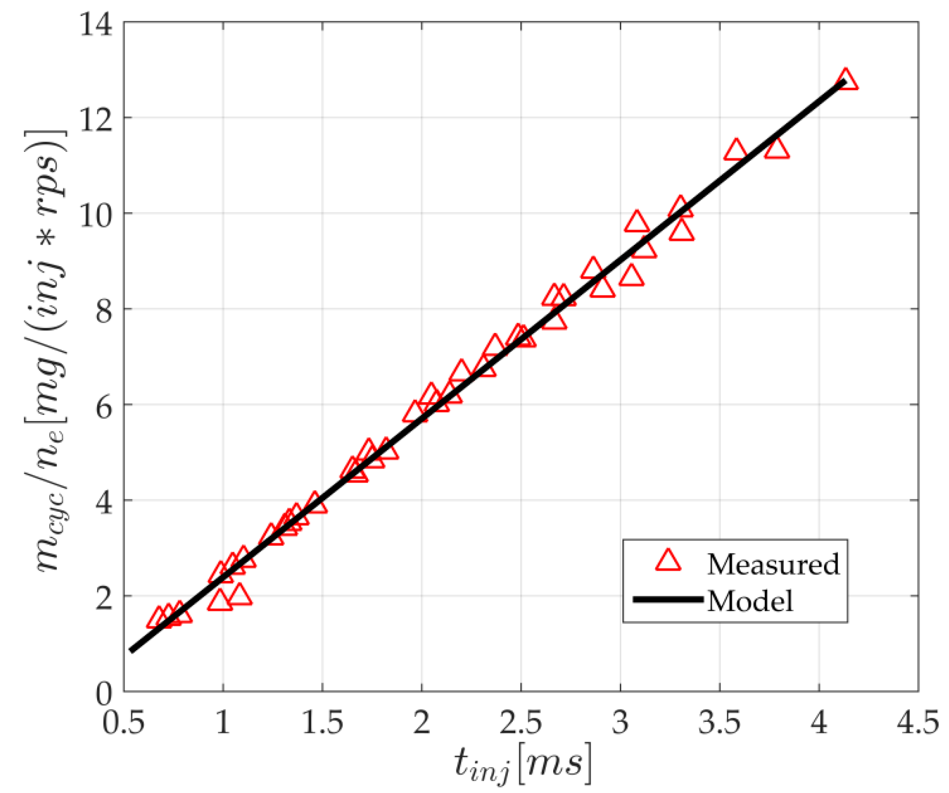
Figure 3.
(a) The measurements of volumetric efficiency in stationary experiment; (b) The model of volumetric efficiency based on intake manifold pressure and engine speed; (c) The tuning result of the air mass into cylinder against the measurement.
Figure 3.
(a) The measurements of volumetric efficiency in stationary experiment; (b) The model of volumetric efficiency based on intake manifold pressure and engine speed; (c) The tuning result of the air mass into cylinder against the measurement.

Figure 4.
Intercooler efficiency model based on engine speed and load.
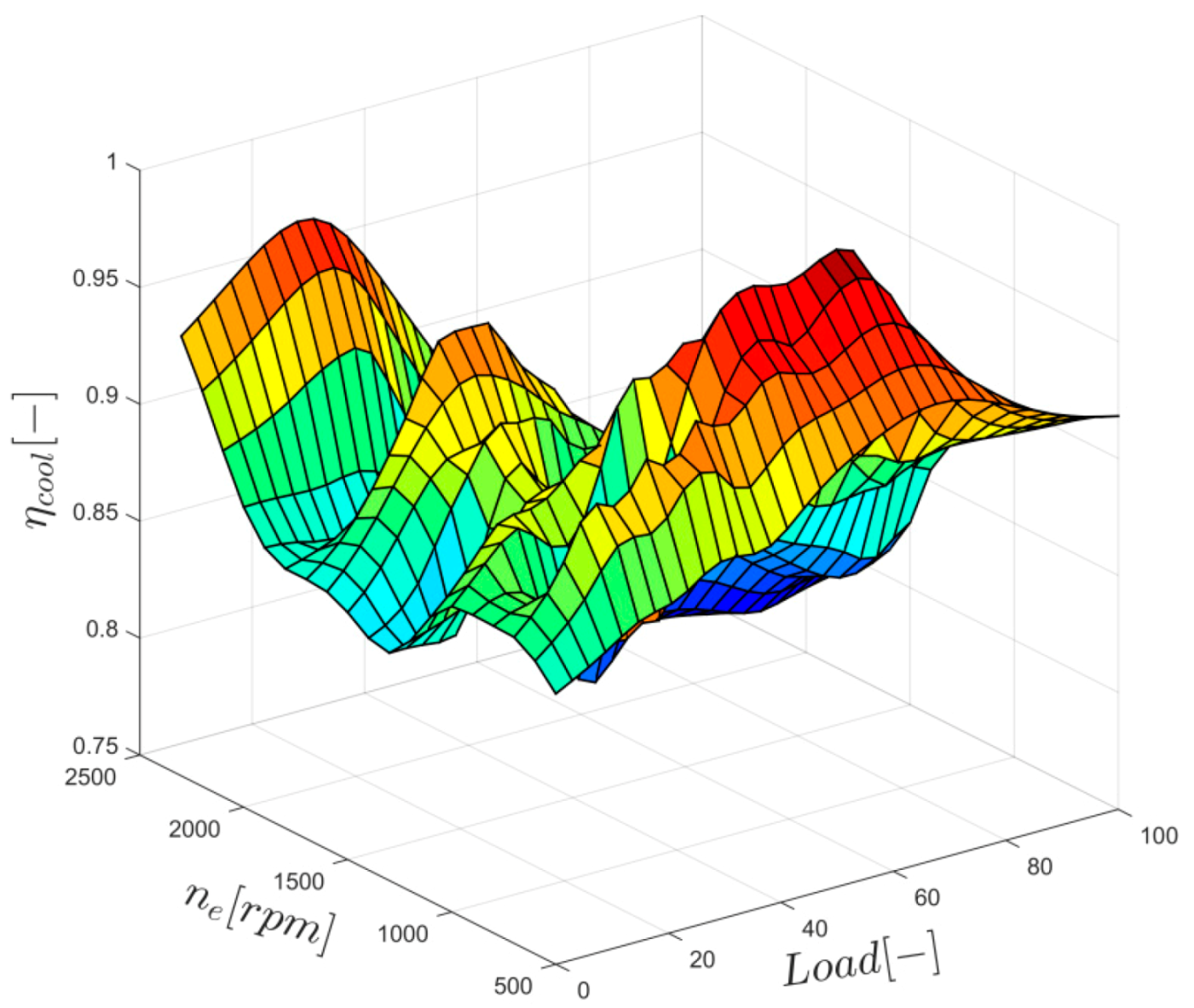
Figure 5.
Comparison of compressor map and modeling result: (a) compressor corrected mass flow; (b) compressor efficiency.
Figure 5.
Comparison of compressor map and modeling result: (a) compressor corrected mass flow; (b) compressor efficiency.

Figure 6.
The result of engine torque generation model against the measurement.

Figure 7.
The tuning result of lubrication oil pressure.
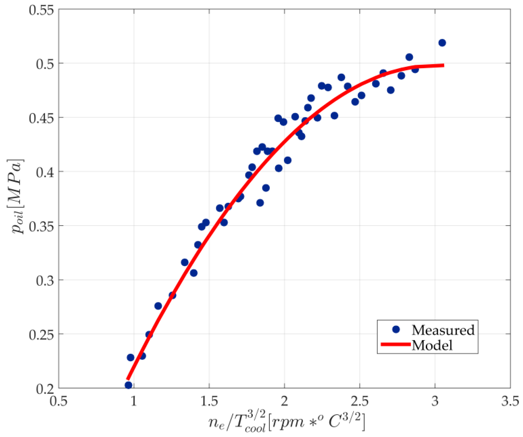
Figure 8.
The validation result of injector model.
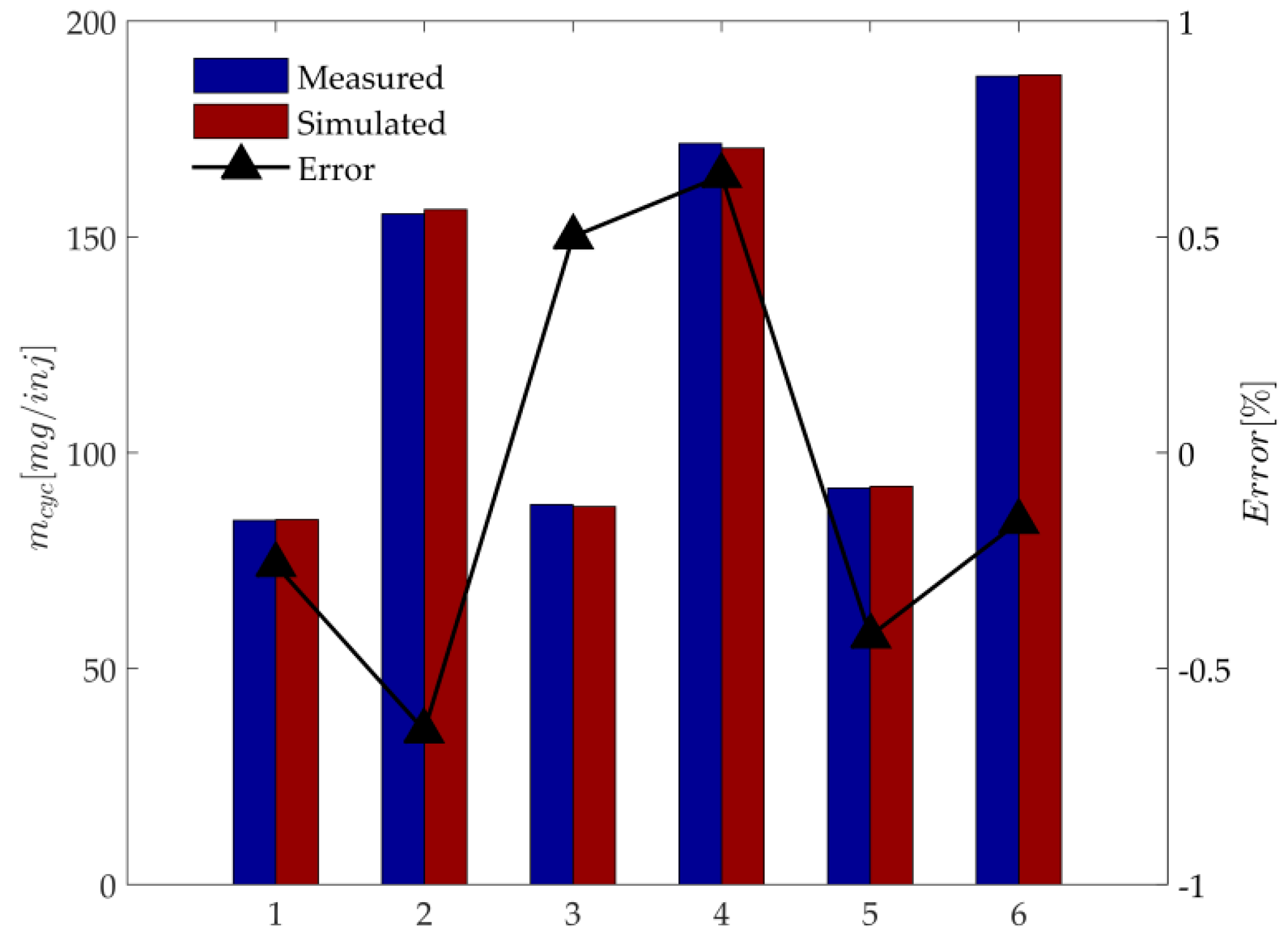
Figure 9.
(a) The validation result of intercooler model; (b) The validation result of intake manifold model; (c) The validation result of air mass into cylinder model; (d) The validation result of effective torque model.
Figure 9.
(a) The validation result of intercooler model; (b) The validation result of intake manifold model; (c) The validation result of air mass into cylinder model; (d) The validation result of effective torque model.

Figure 10.
(a) The validation result of coolant temperature model; (b) The validation result of lubrication oil pressure model.
Figure 10.
(a) The validation result of coolant temperature model; (b) The validation result of lubrication oil pressure model.

Figure 11.
(a) The simulation result of starter model; (b) the simulation result of test bench model.
Figure 11.
(a) The simulation result of starter model; (b) the simulation result of test bench model.

Table 1.
Diesel engine characteristics.
| Characteristics | Value |
|---|---|
| Displacement | 15.8 L |
| Bore × Stroke | 132 mm × 145 mm |
| Number of Strokes | 4 |
| Number of Cylinder | 8 |
| Compression ratio | 17.5 |
| Max enging speed | 2100 rpm |
| Fuel supply system | Electronic Unit Pump |
Table 2.
Measured variable in stationary experiment.
| Measured | Variable |
|---|---|
| Ambient temperature | Ambient pressure |
| Compressor inlet temperature | Compressor inlet pressure |
| Compressor outlet temperature | Compressor outlet pressure |
| Intake manifold temperature | Intake manifold pressure |
| Exhaust manifold temperature | Exhaust manifold pressure |
| Fuel delivery per cycle per cylinder | Injection duration |
| Engine speed | Engine effective torque |
| Coolant temperature | Oil pressure |
© 2017 by the authors. Licensee MDPI, Basel, Switzerland. This article is an open access article distributed under the terms and conditions of the Creative Commons Attribution (CC BY) license (http://creativecommons.org/licenses/by/4.0/).
Share and Cite
MDPI and ACS Style
Yin, J.; Su, T.; Guan, Z.; Chu, Q.; Meng, C.; Jia, L.; Wang, J.; Zhang, Y. Modeling and Validation of a Diesel Engine with Turbocharger for Hardware-in-the-Loop Applications. Energies 2017, 10, 685. https://doi.org/10.3390/en10050685
AMA Style
Yin J, Su T, Guan Z, Chu Q, Meng C, Jia L, Wang J, Zhang Y. Modeling and Validation of a Diesel Engine with Turbocharger for Hardware-in-the-Loop Applications. Energies. 2017; 10(5):685. https://doi.org/10.3390/en10050685
Chicago/Turabian StyleYin, Jinguan, Tiexiong Su, Zhuowei Guan, Quanhong Chu, Changjiang Meng, Li Jia, Jun Wang, and Yangang Zhang. 2017. "Modeling and Validation of a Diesel Engine with Turbocharger for Hardware-in-the-Loop Applications" Energies 10, no. 5: 685. https://doi.org/10.3390/en10050685
Note that from the first issue of 2016, this journal uses article numbers instead of page numbers. See further details here.