
Design of Nonlinear Robust Damping Controller for Power Oscillations Suppressing Based on Backstepping-Fractional Order Sliding Mode


School of Electrical Engineering, Northeast Electric Power University, Jilin 132012, China
*
Author to whom correspondence should be addressed.
Energies 2017, 10(5), 676; https://doi.org/10.3390/en10050676
Submission received: 25 February 2017
/
Revised: 1 May 2017
/
Accepted: 8 May 2017
/
Published: 15 May 2017
(This article belongs to the Special Issue Electric Power Systems Research 2017)
Abstract
:In this paper, a novel nonlinear robust damping controller is proposed to suppress power oscillation in interconnected power systems. The proposed power oscillation damping controller exhibits good nonlinearity and robustness. It can consider the strong nonlinearity of power oscillation and uncertainty of its model. First, through differential homeomorphic mapping, a mathematical model of the system can be transformed into the Brunovsky standard. Next, an extended state observer (ESO) estimated and compensated for model errors and external disturbances as well as uncertain factors to achieve dynamic linearization of the nonlinear model. A power oscillation damping controller for interconnected power systems was designed on a backstepping-fractional order sliding mode variable structure control theory (BFSMC). Compared with traditional methods, the controller exhibits good dynamic performance and strong robustness. Simulations involving a four-generator two-area and partial test system of Northeast China were conducted under various disturbances to prove the effectiveness and robustness of the proposed damping control method.
1. Introduction
Electromechanical oscillations are inherent in large inter-connected power systems between regions [1]. With the expansion of the system scale and increase in transmission power, electromechanical oscillation damping for inter-area mode is decreasing constantly, which causes electromechanical oscillations in power systems to become more serious.
At present, power oscillation damping (POD) for large interconnected power grids has been widely studied, and scholars have proposed numerous improvement approaches. Several means of enhancing the control capability of POD are available. Schemes reported in the literature can be divided into two categories. The first category includes methods that use additional equipment, such as flexible AC transmission systems and high-voltage DC devices, which are becoming practical approaches [2,3,4,5]. However, these schemes require additional equipment. Meanwhile, the second category involves techniques that modify conventional control schemes [6,7,8]. In power systems, damping capability can be improved by way of the first category; however, these approaches increase in cost and complexity. Therefore, control strategies that do not require additional devices are worth studying. A traditional POD controller such as a power system stabilizer (PSS) controller, which has a simple structure and is easy to apply, is designed on the determination model and linear control theory. To enhance damping in power systems, a PSS can be designed on linear matrix inequality [9,10] and H∞ [11]. However, a multi-generator power system is a representative time-varying dynamic system which exhibits parametric uncertainties and is strongly nonlinear. The operating conditions of such systems change constantly, and thus a conventional PSS controller cannot satisfy system requirements.
The linear system control method is based on an accurate model and does not exhibit robustness with the parameters. To compensate for its shortcomings, nonlinear theory is applied to develop a POD controller. The backstepping approach is designed on the Lyapunov nonlinear method; its control function and Lyapunov function can be flexible in selection. This ensures the gradual stability of the disturbance nonlinear system; therefore, this method has been widely used in nonlinear system control [12,13]. However, this method has poor effects on the discontinuous disturbance of the system and nonlinear parameter perturbation.
In recent years, fractional order control has been applied in power systems [14,15,16]. Its main characteristics are high control precision and ease of application. Fractional order sliding mode variable structure control theory (FSMC) has nothing to do with parameter and disturbance. This method has the advantages of fast response speed, robustness, simple structure [17,18,19]. Compared to the integer order, fractional order control has higher control precision, and the system can be more accurately modeled, but this method requires pseudo-linear processing of the original system model. In this paper, the controller was designed based on combining the advantages of the backstepping method and FSMC theory.
The sliding mode control method is more effective for linear parts of systems, but it has difficulty in dealing with nonlinear parts. Multi-generator power systems are complex and stochastic multi-variable nonlinear systems. As stated earlier, designing a controller by traditional methods is difficult, as such controllers are greatly affected by disturbances and uncertainty factors. To compensate for the shortcomings of the linear system control method and the traditional nonlinear control method, extended state observer (ESO) is applied in power systems [20,21,22,23,24]. A combination of FSMC, backstepping, and ESO can obtain a very good damping control effect for nonlinear systems.
To improve the properties of a POD controller, a novel nonlinear ESO-backstepping fractional order SMC (EBFSMC) approach was introduced to design the control law for such controllers. ESO is used to estimate model error and uncertain external disturbance, and eliminate them by feedback. The controller, with feedback based on ESO, was easily designed using the backstepping fractional order SMC (BFSMC) method. The proposed algorithm compensates for the deficiency of the traditional method. The simulation results showed that the method is simple and effective. The POD controller exhibited stronger robustness as well as superior static and dynamic performances compared to the PSS control technique.
The remaining parts of the article are organized as follows. The mathematical model of the system through the differential homeomorphic mapping can be transformed into the Brunovsky standard. Dynamic behavior of multi-machine power systems is discussed in Section 2. Section 3 briefly describes ESO and BFSMC. The EBFSMC scheme is proposed, designed, and analyzed in Section 4. Section 5 explains the self-adaptive wide-area damping control method and control flow. In Section 6, the effectiveness and robustness of the adaptive wide-area damping control method are verified via test systems. Finally, the conclusions of the study are provided in Section 7.
2. Mathematical Modeling of Multi-Machine Power Systems
Interconnected multi-machine systems are composed of n generators. In [1], the seventh-order model of a generator containing excitation control was presented as follows:
where subscript i of variables and parameters indicate the number of generators, i = 1, 2, ..., n. Pei is the electromagnetic power of the ith generator (p.u.); ω0 is the synchronous angular velocity; ωi is the electrical angular velocity of the generator; Pm is the mechanical power; Ti is the inertia time constant of the generator; Di is the damping coefficient; δi is the rotor angle of the generator; δ0 is the synchronous rotor angle of the generator; Idi and Iqi are the d-axis and q-axis stator current of the ith generator, respectively; and are the d-axis and q-axis subtransient electric potential, respectively; and are the d-axis and q-axis transient electric potential, respectively; and are the d-axis and q-axis subtransient reactance, respectively; x’di and x’qi are the d-axis and q-axis transient reactance, respectively; and are the d-axis and q-axis open-circuit subtransient time constant, respectively; and are the d-axis and q-axis open-circuit transient time constant, respectively; Efi is the excitation electric potential; Te and KA are the time delay and control gain in excitation control, respectively; Vref and V are the reference and actual voltage; Vpss is the reference voltage of the PSS damping control input. Pei and Idqi can be respectively expressed as follows:
where xdqi are the d-axis and q-axis synchronous reactance of the ith generator, respectively; δij is a relative angle of the ith and jth generators; Gii and Bii are the auto-admittance and auto-conductance of the ith generator, respectively; Gij and Bij are the mutual-admittance and auto-conductance of the ith and jth generators, respectively.
Through differential homeomorphic mapping [25], the model of generators can be transformed into Equation (2) through coordinate transformation.
Then, as per precise linearization knowledge, Equation (2) can be derived as follows:
where , expression of , , are detailed in Appendix A.
Additionally,
As shown in the above derivation, different order model of the generators can be written in general formula form in the following:
where the x is the ith state variables, and u is the control input. Equation (7) can provide a model for the follow-on controller designation.
3. Design Principles of EBFSMC
3.1. Feedback Linearization Based on ESO
ESO is an important component of auto-disturbance-rejection controllers [23,24]. As an observer, ESO can evaluate uncertainties and simultaneously compensate disturbances. The nth order nonlinear uncertain system that is affected by several unknown external disturbances is expressed as follows [23,24]:
where is an unknown function; w1(t) is an unknown disturbance; x is a measurement state variable; is the controlling input; and b is the coefficient of the control input.
Let
Then, the expansion state equation (i.e., Equation (8)) is given by
where h(t) is an unknown function.
Next, the expanded state observer can be constructed as follows:
where z1(t), …, zn+1(t) are the outputs of ESO, e01 = z1 − x1. g1(e01), ..., gn+1(e01) are the opportunely structured nonlinear correction functions.
Then, based on Equations (10) and (11), Equation (12) can be obtained as follows:
where e0i = zi − xi, ().
Regarding the discretionarily varying h within limits, the authors of [15] testified that if the nonlinear successive functions g1(e01), ..., gn+1(e01) are selected, then Equation (12) is steady with respect to the origin. That is, by choosing functions g1(e01), ..., gn+1(e01), the states of Equation (11) can follow the homologous states in Equation (10); i.e.,
As per Equation (9), the total of the uncharted functions and the external disturbance w1(t) in Equation (1) is . xn+1(t) is considered as an extended state. are used to represent the dynamic properties of Equation (1), and thus, ESO can be identified for the nonlinear system equation (i.e., Equation (11)).
The control variable is selected as follows:
In this paper, the ESO is used to estimate the model error and the uncertain external disturbance, then eliminate them by feedback. Due to the difficulty in processing nonlinear parts for FSMC, it can make use of ESO to strengthen the processing nonlinear part of the system. Thus, it can enhance the resistance perturbation ability of the algorithm for dealing with a nonlinear problem.
3.2. Fractional Calculus Theory
Fractional order calculus is the generalized form of integer order differential and integral calculus [26,27,28,29]. Fractional calculus has many definitions. In this study, the Caputo fractional order calculus was used.
The Caputo fractional order differential definition as follows from [14]:
where , ; and n is an integer.
Similarly, fractional integral is defined as follows:
The main idea of the fractional integral is to create a functional operator D. The order ε of D is not confined to the integer, particularly when the concepts of differentiation (when ε is positive) and integration (when ε is negative) are promoted. The follow-up can be abbreviated as .
The depth of the integer order can be expanded by the fractional order. It not only has the effect of an integer order, but also has the effect the integer order does not have. The low fractional order controller can have the effect of a high-order integer order. It reduces the difficulty of controller design, and improves practicability.
4. Proposed BFSMC POD Controller Based on ESO
The principle of the new damping controller—which can be used in interconnected power systems—is presented in the following paragraphs.
In FSMC design, the FSMC law and switching function are mainly considered [17]. Figure 1 shows the control structure of the EFSMC applied in the damping controller.
Based on Equation (1), variations and Vpss can be defined as state and input variations, respectively.
The specific design is as follows.
Step 1: Constructing the sliding surface and backstepping approach. If the tracking value of the state variables is xref, then the tracking error is presented as follows:
The definition of the sliding mode surface formula is as follows:
The Lyapunov function is defined as Equation (19):
By deriving Equation (19), we can obtain
Let
Then, Equation (21) is added into Equation (20), which yields
Let
Then, Equation (23) is added into Equation (22), which yields
The Lyapunov function is defined as Equation (25):
By deriving Equation (25), we can obtain
Let
Then, Equation (27) is added into Equation (26), which yields
Let
As per Equation (28) and Equation (29), it is
The Lyapunov function is defined as Equation (31):
By deriving Equation (31), we can obtain
Let
As per Equations (24), (26), (32), and (33), it is
Let
Then
The Lyapunov function is defined as Equation (37):
By deriving Equation (37), we can obtain
Let
As per Equations (36), (38), and (39), it is
Let
Then
The Lyapunov function is defined as Equation (43):
By deriving Equation (43), we can obtain
Let
As per Equations (44) and (45), it is
If ks1, ks2, ks3, ks4, ks5, ks6 and c1i, c2i, c3i, c4i, c5i are negative, would keep negative definite, and the control strategy could guarantee the stability of the controlled system.
Step 2: Designing ESO. Given that pre-control variable contains many parameters and system state variables, ESO is introduced to simplify these components.
The pre-control variable is presented as follows:
where Uf is Vpss. is the pre-control variables and the derivation process is detailed in Appendix B. The expression of will be introduced further in Step 3.
Regarding the first-order state equation (i.e., Equation (47)), the structure of the second-order extended state observer is used to estimate a and b, which contains many parameters and state variables. The corresponding formula is expressed as follows:
where is used to estimate variable ; and is an extended variable which is used to estimate variable . In addition, is observable. The fe function is a continuous power law function with a linear segment near the origin. It avoids the high-frequency chattering phenomenon. Uncertain factors can be dynamically compensated by . are adjustable parameters.
The nonlinear function is defined as follows:
where e, α, and δ are the control parameters; and sign is the symbol function. δ > 0, 0 < α < 1 are an important property of the function.
Step 3: Selection of BFSMC Law. For Equation (47) after ESO feedback, if the estimation error of ESO is not considered, we can approximate the formula of the system as follows:
where the estimated variant b is the coefficient of the control variable. Uf is before the estimation.
As shown in Equation (48), the function of ESO is to redistribute the variable on the right side of Equation (48), which can cause the original control variables with the variable coefficient in ESO to transform into a linear combination of the variable and constant coefficient.
Thereby, the system parameters and the state variable problem can be omitted, and consequently, feedback control is simplified.
By comparing Equation (48) with Equation (50), the expression of the control variables can be obtained, and the corresponding formula is as follows:
where the expressions of a1—a5, b1—b5 are found in Appendix C.
Thus, the control law can be defined as follows:
where u = Uf, and z2 is extended variable.
The schematic of the proposed BFSMC based on ESO is shown in Figure 1.
5. Proposed Control Scheme for Damping Oscillation and Control Flow
The proposed EBFSMC damping controller was designed as described in Section 4. With regard to the proposed control scheme for damping oscillation, there were also some important issues such as the identification of low-frequency oscillation and the selection of input signals for wide-area damping controller (WADC).
5.1. Parameter Identification of Low-Frequency Oscillation Based on Stochastic Subspace Identification (SSI)
To better design a WADC, low-frequency oscillation parameters and the dominant inter-area oscillation mode should be extracted from the measured signal. SSI is used to extract low-frequency oscillation parameters and mode shapes from measured signals, as it exhibits good robustness and numerical simplicity. Though there are other parameter identification methods including wavelet transform [30], Hilbert–Huang transform [31], spectral methods [32], etc., those are difficult-to-extract oscillation mode shapes. SSI was used as it has high accuracy and can extract oscillation mode shapes.
SSI is divided into two parts. The numerical algorithm for subspace state space system identification is used first to estimate the state space model, then modal analysis and mode shape identification are performed. The specific calculation process is detailed in [1]. Modal parameters and mode shape can be obtained from the measured signal.
5.2. Selection and Analysis of Input Signals for WADC
By using synchronized signals from a wide-area measurement system (WAMS), online methods have been proposed to extract online electromechanical oscillation parameters and provide damping control; for example, Prony [33] and SSI [34,35,36] analyses.
The signals obtained from WAMS should be measurable and should contain information on oscillation, such as the angular and speed difference of generators, active power, etc. These measured signals have certain controllability and reliability. In practice, a significant time delay is observed in wide-area signals of WAMS and transmission communication networks. When these signals are used for damping control and analysis, the influence of time delay should be considered. In general, the time delay is from 100 ms to 300 ms. Good control effect can still be achieved using EBFSMC within the allowed time delay. In addition, the wide-area feedback used in WADC may be introduced into noise during the transmission process. Thus, this factor should also be considered in controller design. It should also have good damping effect, particularly under a certain amount of noise. Therefore, the WADC designed in this study considered the above-mentioned factors.
5.3. Control Flow of the Proposed Damping Control Scheme
The flow graph of the proposed control method for damping oscillation—which mainly consists of the EBFSMC described in previous sections—is presented in Figure 2. As shown in the figure, the main steps are as follows.
- (1)
- First, fractional order sliding mode is applied through a linear combination between the state variables and the fractional order based on Equation (20).
- (2)
- Second, the Lyapunov function is defined based on backstepping approach in Equation (21).
- (3)
- The expression that contains control variables can be obtained by deriving the Lyapunov function based on Equations (47) and (48).
- (4)
- Construct ESO and redistribute the expression containing control variables in Equation (48).
- (5)
- As per the negative form of the Lyapunov function derivative, the expression with control variables can be obtained in Equation (51).
6. Simulation Results and Discussion
6.1. Four-Machine Two-Area Test System
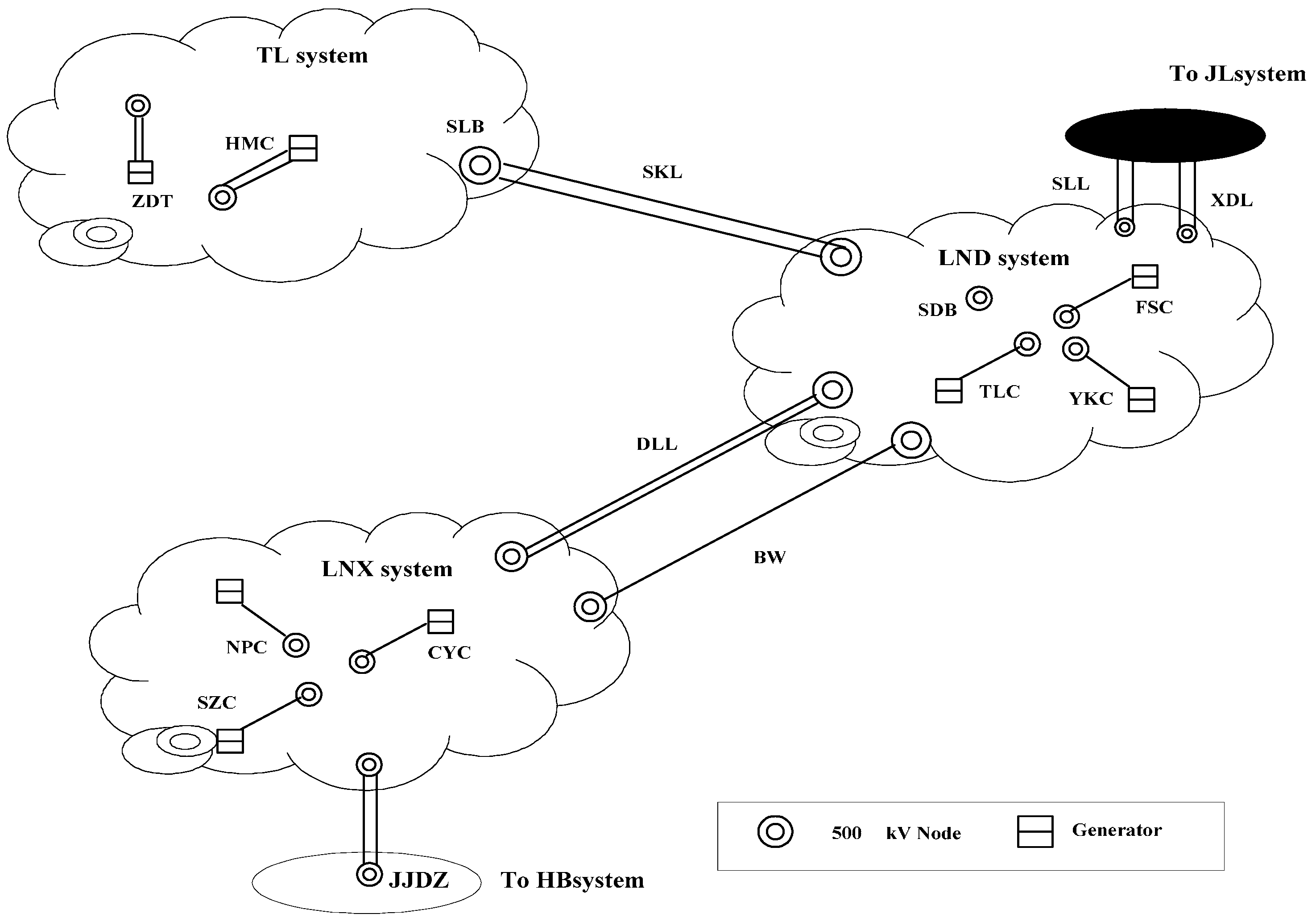
The characteristics of the proposed wide-area damping control approach based on EBFSMC were estimated using a four-machine two-area test system (Figure 3). Data on the system can be obtained from [1]. The areas of the system are referred to as Areas 1 (G1–G2) and 2 (G3–G4). The PSS is equipped in G2.
To verify the effectiveness of the proposed damping control approach, the operation scheme—which is the power flow of the tie lines (lines 3–13 a and lines 3–13 b) from Areas 1–2—is approximately 400 MW. The inter-area mode is (G1–G2) and (G3–G4), which is an important mode affected by several disturbances. For example, Case a: a three-phase fault is at bus 101 for 200 ms. Case b: a three-phase short circuit fault under tie line overload. When the other parameters are constant, the power of the tie line is strengthened to approximately 100 MW by transferring the load from bus 3 to bus 13.
To verify the effect of the proposed control strategy, local PSS (LPSS) [1], ESO-H∞(ESOH) [23], and EBFSMC controller were analyzed in the following.
6.1.1. Characteristics of Oscillation Mode Extraction
Through measuring the angular frequency signal of different generators, low-frequency oscillation parameters and the state of system are identified by SSI. The results of oscillation mode presented in Table 1 were obtained by SSI. This method can recognize low-frequency oscillation modes, such as the inter-area oscillation mode. In this study, special attention was focused on analyzing the inter-area oscillation mode. The theoretical mode of this inter-area mode was (G1–G2) and (G3–G4). As shown in Table 1, the inter-area mode was inspired in both two cases.
The Prony method was introduced to summarize the important mode from the active power signal of the tie line. The rotor angular velocity difference of G1–G3 wG13, rotor angular velocity of G3 wG3, and the active power of line 3–13 a P3~13 a were selected. The information obtained using the Prony method is provided in Table 2. As shown in Table 1 and Table 2, the mode identification results obtained using the Prony method are similar to those acquired using SSI. However, when compared with the Prony method, SSI not only showed a high stability and accuracy in results, but also exhibited mode shapes.
6.1.2. Effectiveness of the Proposed Wide-Area Control Approach for Damping Power Oscillation
As shown in Table 1, the important inter-area oscillation mode was detected under a disturbed condition. Meanwhile, relevant oscillation generator clusters were identified. Based on remote input information from measuring data, WADCs were built. As shown in Table 1, the damping system was improved when using the proposed method, and the mode shape was invariant when using the LPSS, ESOH and EBFSMC controller.
As shown in Figure 4 and Figure 5, the effectiveness of the inter-area oscillation control using LPSS, ESOH, and EBFSMC under a disturbed situation is demonstrated.
Through feedback linearization and solving Riccati equation, the control law of ESOH can be obtained as follows:
The control parameters of the EBFSMC regulator are provided in Table 3, Table 4 and Table 5. Control parameters of the ESOH regulator are shown in Table 6.
The tie line flow for system responses under Cases a and b are shown in Figure 4a,b, respectively. Under the important inter-area power oscillation mode, the system would spend more time settling down when LPSSs and ESOH were installed. As shown in Figure 4, oscillations were restrained immediately under nearly the same situation using the proposed EBFSMC. Meanwhile, as shown in Table 1, the damping system obviously increased when EBFSMC was adopted. Compared with the linear robust method and traditional PSS, the proposed method had better adaptability and control effect for nonlinear systems. Although the proposed control system is rather complex, the proposed method is more appropriate for complex nonlinear systems, and the stability is considered when the EBFSMC as designed. At the same time, it has a certain anti-noise and the ability to resist interference.
The effectiveness of the WADCs has been proven to be worse without EBFSMC. The proposed EBFSMC scheme works efficiently.
6.1.3. Influence of the Proposed WADC under a Time Delay
A significant time delay of wide-area signals is present in WAMS and transmission communication networks. When these signals are used for damping control and analysis, the influence of time delay should be considered. To verify the robustness of the proposed WADC under a time delay, different time delay periods of power angle signal were used for comparison and analyses. The results are presented in Figure 5a. As shown in Figure 5a, good results were obtained under certain time delay periods. This finding demonstrates the robustness of the proposed WADC under such conditions.
6.1.4. Influence of the Proposed WADC under Noise
To consider noise in the process of communication, the effectiveness of the proposed scheme in a noisy environment was also verified in this study. Gaussian white noise with a mean of 0 and 0.2 covariance was introduced into the feedback power angle signal. The results are presented in Figure 5b. As shown in the active power of G1, the proposed method could also effectively achieve damping control.
6.1.5. Influence of System Performance under Parameter Variation
To validate the influence of the experiment results caused by ε, the effect of damping under different ε values were analyzed. The results are provided in Figure 5c.
The situations of different ε values are shown in Figure 5c. The values of ε are −0.0005, −0.005, and −0.05. As shown in Figure 5c, the larger the value of ε, the faster the adjustment speed in general. The proposed controller demonstrated strong robustness, and changes in state variables caused by parameter perturbations could be controlled within a reasonable range.
This study proved that ε ranges from 0 to −0.1 under numerous simulation experiments. Regarding the limitation of the parameters, the proposed scheme exhibited better performance under larger parameters. As parameter variation increased, damping effect was enhanced. However, parameters must be restricted. If they exceed the limitations, then the power system may become unstable. Hence, appropriate parameters should be chosen. In this study, ε = −0.005 was selected for the experiments. The test curves are presented in Figure 4 and Figure 5.
6.1.6. Influence of System Performance under System Parameter Variation
To validate the influence of the experiment results caused by system parameter variation, the effect of damping under different disturbance amplitudes of were analyzed. The results are provided in Figure 5d. As shown in Figure 5d, the system parameters were disturbed under certain amplitude, and had little influence on control effect. This shows that the proposed method has certain robustness for parameter variation.
6.2. The Partial Test System of Northeast China
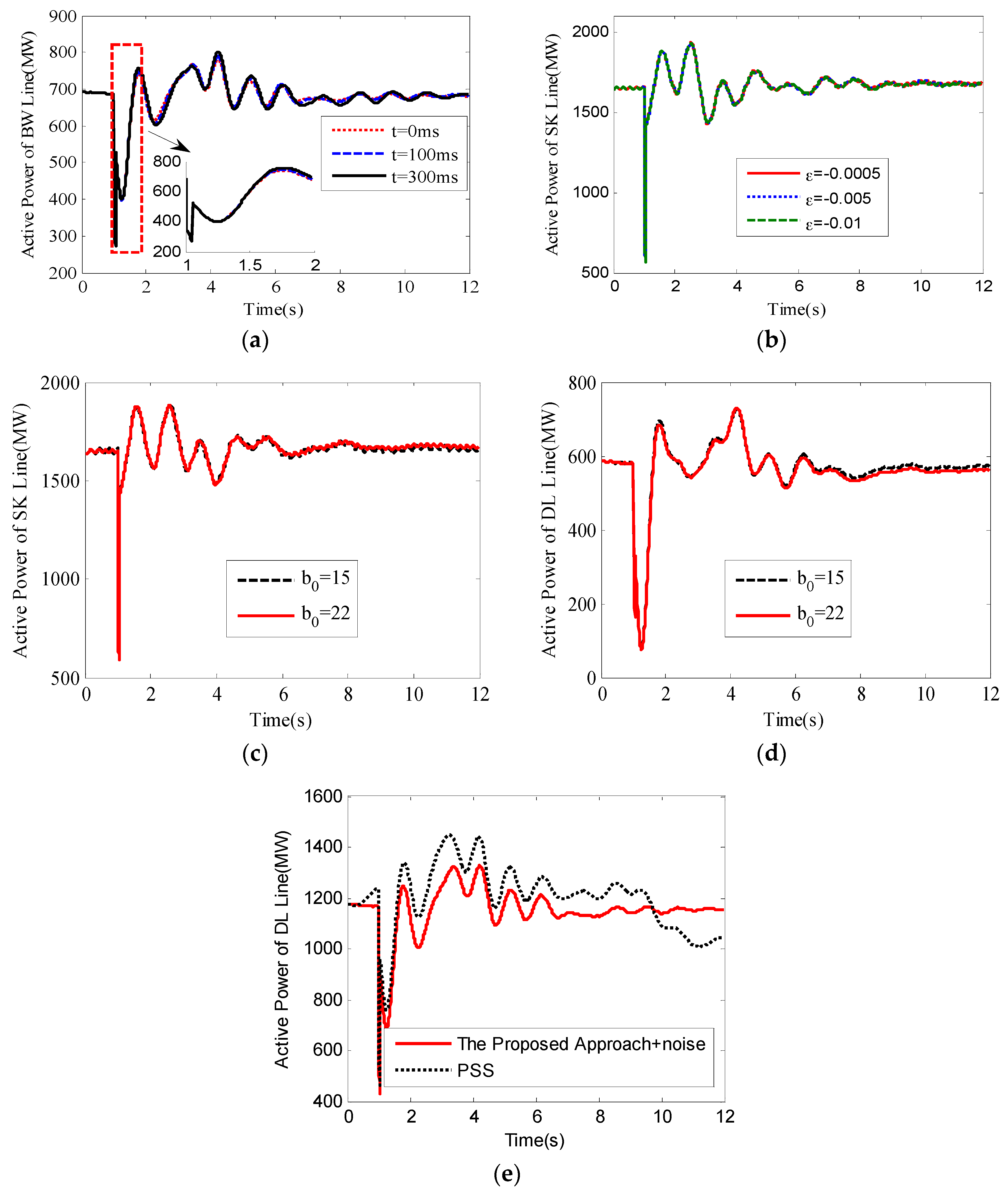
Part of the Northeast transmission network in China, with 90 generators and 306 buses, was investigated by simulation. Figure 6 shows part of the Northeast network where different areas are connected through 500 kV transmission lines. To test the effectiveness of the proposed method, the following operation condition was considered. This important mode is affected by several disturbances. To demonstrate the proposed controller, a variety of system operating conditions were considered. For example, a three-phase fault was present at bus SDB in the LND system for 50 ms. Case a: a power flow of 1648 MW in the SK line and a power flow of 1174 MW in the DL line. Case b: part load of LND system were reduced. Next, we obtained a power flow of 1648 MW in the SK line and a power flow of 1584 MW in the DL line.
6.2.1. Property of Oscillation Mode Extraction
WAMS were placed in different areas to measure the angular speed signal of different generators and to identify low frequency oscillation parameters and the modal shape of the system. The results shown in Table 7 were obtained by SSI. As shown in the table, the proposed method could recognize inter-area oscillation modes. The inter-area mode {ZDT, HMC, YKC, FSC, TLC} and {SZC, JJDZ} in Case a, {ZDT} and {FSC, TLC, SZC, JJDZ, HMC, YKC} in Case b were inspired by disturbances and extracted by SSI.
6.2.2. Effectiveness of the Proposed Wide-Area Control Approach for Damping Power Oscillation
As indicated in Table 6, important inter-area oscillation modes were detected under a disturbed condition, and relevant power oscillation generator clusters were identified. ZDT was implemented as the damping controller.
The damping effect on the active power of the DL line under Case a and Case b are shown in Figure 7a,b, respectively. Power oscillation could be controlled effectively under different operating conditions.
As shown in Figure 7 and Figure 8, the effectiveness of the inter-area oscillation control using wide-area PSS, ESOH, and EBFSMC under a disturbed situation is demonstrated. For the proposed controller, angular speed signals of ZDT and JJDZ in two areas were selected as the control input, which were measured by WAMS placed in two areas, respectively. The sampling frequency of WAMS was 100 Hz. The related parameters of the controller design, the ESO observer, and FSMCB regulator parameters are shown in Table 8, Table 9 and Table 10.
The active power of the tie-line with PSS, ESOH, and EBFSMC are plotted in these figures. Under important inter-area power oscillation modes, the system oscillation will spend more time settling when PSS and ESOH are installed. As shown in Table 7, the damping system was improved when using the proposed method. The figures also indicate that oscillations may be restrained immediately when using the proposed EBFSMC. Meanwhile, as shown in Table 7, the damping system obviously increased when EBFSMC was adopted. As shown in Figure 8, the proposed EBFSMC scheme could work well under different time delay periods, noise, and varying uncertainties in control parameters. As shown in Figure 8c,d, the proposed method had certain robustness for parameter variation.
7. Conclusions
A nonlinear power oscillation damping controller was introduced in this paper, which was designed by combining the advantages of ESO and BFSMC theory to reduce power oscillation damping in power systems. Once power oscillation is detected, the oscillation mode will first be recognized efficiently using the SSI algorithm. According to important oscillation modes with insufficient damping, power oscillation can be reduced by EBFSMC. Internal and external disturbances in the system can be dynamically compensated by ESO, which reduces the complexity of the controller and enables it to exhibit strong practicability and robustness. The controller has a simple structure and is designed on the backstepping fractional order sliding mode. In addition, the proposed EBFSMC exhibits the advantages of rapid response and insensitivity to disturbances. The simulation results demonstrated that the proposed power oscillation damping control scheme reduces power oscillation. The effectiveness of the proposed algorithm has also been verified.
Conflict of Interests
The authors declare no conflict of interest.
Acknowledgments
The authors are very grateful to the reviewers and the editor for their valuable comments that helped improve the presentation of the article. This work was supported by the National Key Research and Development of China Program “The technologies and equipment in smart grid” (2016YFB0900100) and the National Natural Science Foundation of China (No. 51377017).
Author Contributions
Cheng Liu put forward to the main idea and designed the entire structure of this paper. Guowei Cai guided the experiments and paper writing. Jiwei Gao made good suggestions in the article modification process and revised the paper. Deyou Yang proposed the revised opinion.
Appendix A
Appendix B
Appendix C
References
- Kundur, P. Power System Stability and Control; McGraw-Hill: Hightstown, NJ, USA, 1994; pp. 154–196. [Google Scholar]
- Jiang, P.; Feng, S.; Wu, X. Robust design method for power oscillation damping controller of STATCOM based on residue and TLS-ESPRIT. Int. Trans. Electr. Energy Syst. 2014, 24, 1385–1400. [Google Scholar] [CrossRef]
- Li, Y.; Christian, M.G.; Rehtanz, S.R. Wide-area robust coordination approach of HVDC and FACTS controllers for damping multiple interarea oscillations. IEEE Trans. Power Deliv. 2012, 3, 1096–1105. [Google Scholar] [CrossRef]
- Khalilian, M.; Mokhtari, M.; Golshannavaz, S. Distributed static series compensator (DSSC) for subsynchronous resonance alleviation and power oscillation damping. Eur. Trans. Electr. Power 2012, 5, 589–600. [Google Scholar] [CrossRef]
- Sui, X.C.; Tang, Y.F.; He, H.B. Energy-storage-based low-frequency oscillation damping control using particle awarm optimization and heuristic dynamic programming. IEEE Trans. Power Syst. 2014, 5, 2539–2548. [Google Scholar] [CrossRef]
- Ganjefar, S.; Alizadeh, M. A novel adaptive power system stabilizer design using the self-recurrent wavelet neural networks via adaptive learning rates. Int. Trans. Electr. Energy Syst. 2013, 23, 601–619. [Google Scholar] [CrossRef]
- Ruiz-Vega, D.; Messina, A.R.; Pavella, M. Online assessment and control of transient oscillations damping. IEEE Trans. Power Syst. 2004, 3, 1038–1047. [Google Scholar] [CrossRef]
- Wang, D.; Mevludin, G.; Louis, W. Trajectory-based supplementary damping control for power system electromechanical oscillations. IEEE Trans. Power Syst. 2014, 6, 2835–2845. [Google Scholar] [CrossRef]
- Wu, H.X. Evaluation of time delay effects to wide-area power system stabilizer design. IEEE Trans. Power Syst. 2004, 4, 1935–1941. [Google Scholar] [CrossRef]
- Deng, J.C.; Zhang, X.P. Robust damping control of power systems with TCSC: A multi-model BMI approach with H2 performance. IEEE Trans. Power Syst. 2014, 4, 1512–1521. [Google Scholar] [CrossRef]
- Chaudhuri, B. Mixed-sensitivity approach to H∞ control of power system oscillations employing multiple FACTS devices. IEEE Trans. Power Syst. 2003, 3, 1149–1156. [Google Scholar] [CrossRef]
- Morawiec, M. The Adaptive backstepping control of permanent magnet synchronous motor supplied by current source inverter. IEEE Trans. Ind. Inform. 2013, 2, 1047–1055. [Google Scholar] [CrossRef]
- Yang, P.H.; Wwi, Y.L.; Liu, W.Y. An adaptive damping controller design based on back-stepping and variable structure method. Power Syst. Prot. Control 2011, 24, 96–100. [Google Scholar]
- Indranil, P.; Saptarshi, D. Kriging based surrogate modeling for fractional order control of microgrids. IEEE Trans. Smart Grid 2015, 1, 36–44. [Google Scholar]
- Sanjoy, D.; Lalit, C.S.; Nidul, S. Automatic generation control using two degree of freedom fractional order PID controller. Int. J. Electr. Power Energy Syst. 2014, 58, 120–129. [Google Scholar]
- Ma, D.W.; Sun, B.; Luo, Z.Y. Design generator excitation controller based on fractional order sliding mode and extended state observer. Water Resour. Power 2015, 4, 167–169. [Google Scholar]
- Liu, J.K. Matlab Simulation for Sliding Mode Control; Tsinghua University Press: Beijing, China, 2005; pp. 12–35. [Google Scholar]
- Farzad, P.; Farshad, F.; Constantine, J. Local sliding control for damping interarea power oscillations. IEEE Trans. Power Syst. 2004, 2, 1123–1134. [Google Scholar]
- Feng, Y.; Yu, X.; Han, F. High-order terminal sliding mode observer for parameter estimation of a permanent magnet synchronous motor. IEEE Trans. Ind. Electron. 2013, 60, 4272–4280. [Google Scholar] [CrossRef]
- Li, T.Y.; Zhang, Z.H.; Chen, F. Design of nonlinear robust controller of HVDC power transmission system based on extended state observer and terminal sliding mode control. Power Syst. Technol. 2012, 10, 190–195. [Google Scholar]
- Liu, H.X.; Li, S.H. Speed control for PMSM servo system using predictive functional control and extended state observer. IEEE Trans. Ind. Electron. 2012, 2, 1171–1183. [Google Scholar] [CrossRef]
- Guo, B.Z.; Wu, Z.H.; Zhou, H.C. Active disturbance rejection control approach to output-feedback stabilization of a class of uncertain nonlinear systems subject to stochastic disturbance. IEEE Trans. Autom. Control 2016, 21, 1613–1618. [Google Scholar] [CrossRef]
- Han, J.Q. Active Disturbance Rejection Control Technique; National Defense Industry Press: Beijing, China, 2008; pp. 25–69. [Google Scholar]
- Han, J.Q. From PID to active disturbance rejection control. IEEE Trans. Ind. Electron. 2009, 3, 900–906. [Google Scholar] [CrossRef]
- Li, T.Y.; Zhu, J.H.; Yuan, M.Z. Design of A Robust Excitation Controller Based on Differential Homeomorphic Mapping and Extended State Observer. Power Syst. Technol. 2012, 36, 131–135. [Google Scholar]
- Podlubny, I. Fractional-order systems and PIλDμ-controllers. IEEE Trans. Autom. Control 1999, 1, 208–214. [Google Scholar] [CrossRef]
- Samko, S.G.; Kilbas, A.A.; Marichev, O.I. Fractional Integrals and Derivatives; Gordon and Breach: Yverdon, Switzerland, 1993; pp. 25–69. [Google Scholar]
- Luo, Y.; Zhang, T.; Lee, B.J. Fractional-order proportional derivative controller synthesis and implementation for hard-disk-drive servo system. IEEE Trans. Control Syst. Technol. 2014, 22, 281–289. [Google Scholar] [CrossRef]
- Pan, I.; Das, S. Intelligent Fractional Order Systems and Control; Springer: Berlin, Germany, 2013; pp. 15–65. [Google Scholar]
- Avdakovica, S.; Nuhanovicb, A.; Kusljugic, M. Wavelet transform applications in power system dynamics. Electr. Power Syst. Res. 2012, 2, 237–245. [Google Scholar] [CrossRef]
- Messina, A.R.; Vittal, V. Nonlinear, non-stationary analysis of interarea oscillations via Hilbert spectral analysis. IEEE Trans. Power Syst. 2006, 3, 1234–1241. [Google Scholar] [CrossRef]
- Ostojic, D.R. Spectral monitoring of power system dynamic performances. IEEE Trans. Power Syst. 1993, 2, 445–451. [Google Scholar] [CrossRef]
- Grund, C.E.; Paserba, J.J.; Hauer, J.F.; Nilsson, S.L. Comparison of Prony and eigenanalysis for power system control design. IEEE Trans. Power Syst. 1993, 3, 964–971. [Google Scholar] [CrossRef]
- Ghasemi, H.; Canizares, C.; Moshref, A. Oscillatory stability limit prediction using stochastic subspace identification. IEEE Trans. Power Syst. 2006, 2, 736–745. [Google Scholar] [CrossRef]
- Zhang, P.; Yang, D.Y.; Chan, K.W. Adaptive wide-area damping control scheme with stochastic subspace identification and signal time delay compensation. IET Gener. Transm. Distrib. 2012, 9, 844–852. [Google Scholar] [CrossRef]
- Reynders, E.; Roeck, G.D. Reference-based combined deterministic-stochastic subspace identification for experimental and operational modal analysis. Mech. Syst. Signal Process. 2008, 3, 617–637. [Google Scholar] [CrossRef]
Figure 1.
Schematic of the proposed backstepping fractional order sliding mode variable structure control theory (BFSMC) based on extended state observer (ESO).
Figure 1.
Schematic of the proposed backstepping fractional order sliding mode variable structure control theory (BFSMC) based on extended state observer (ESO).
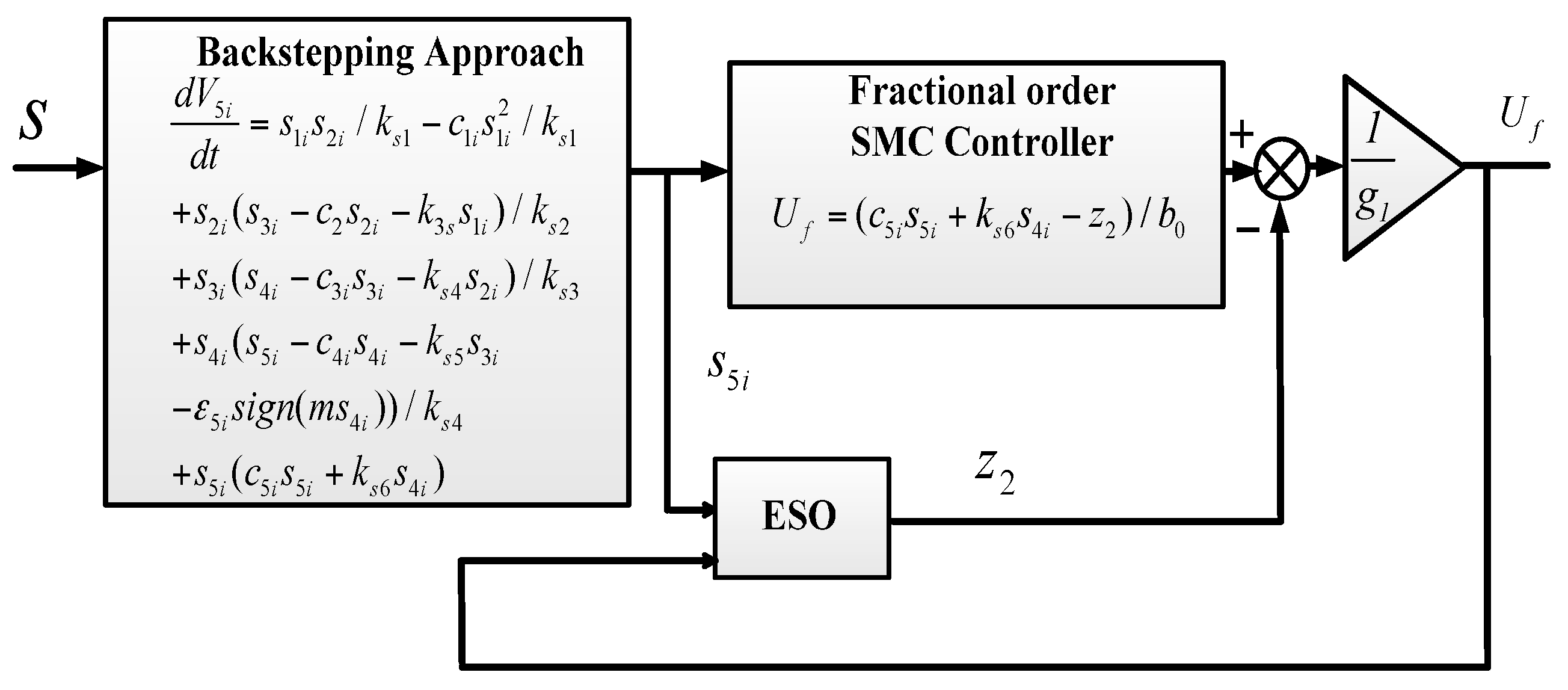
Figure 2.
Flow diagram of the proposed BFSMC based on ESO.
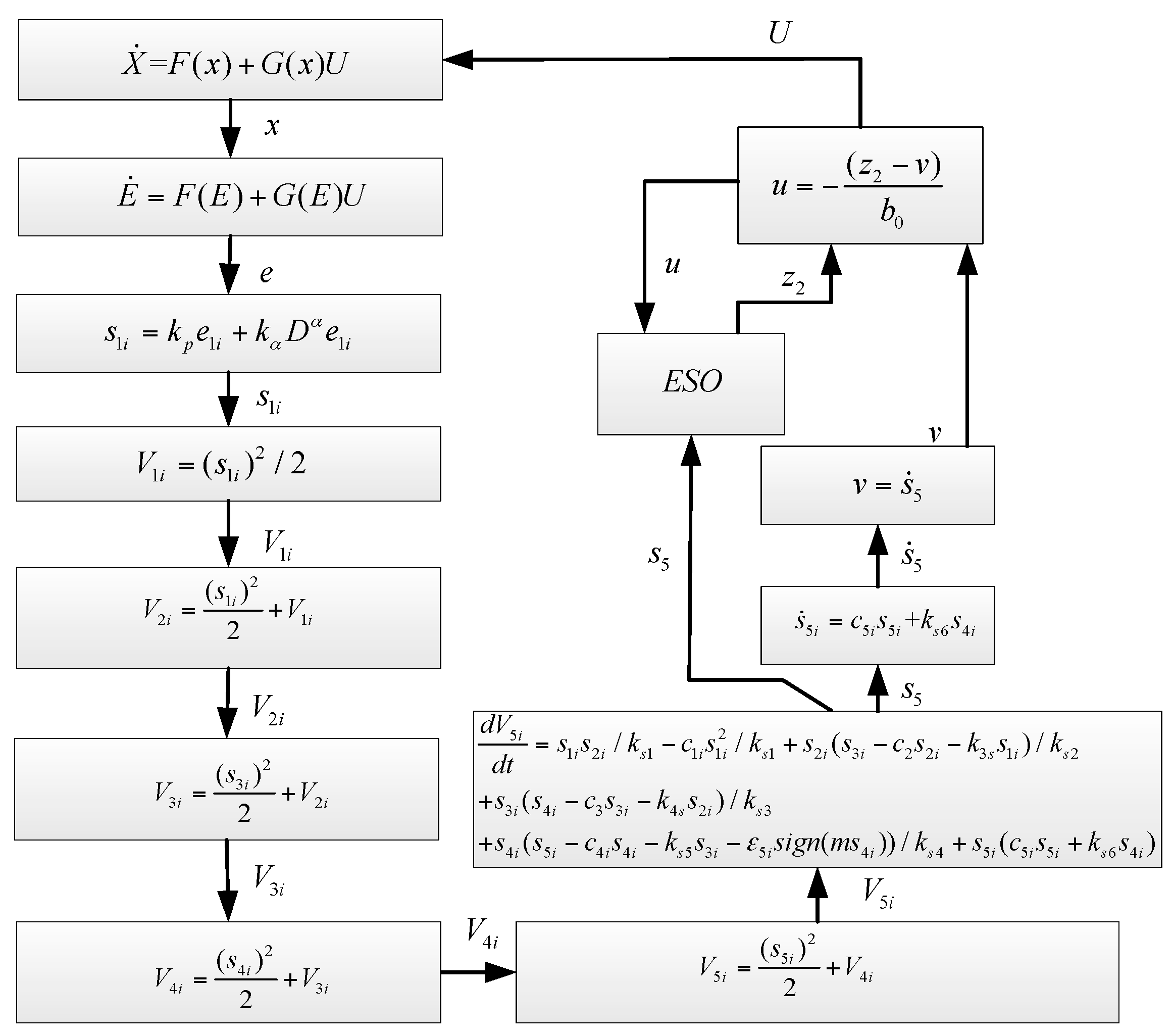
Figure 3.
Illustration of the four-machine two-area test system.
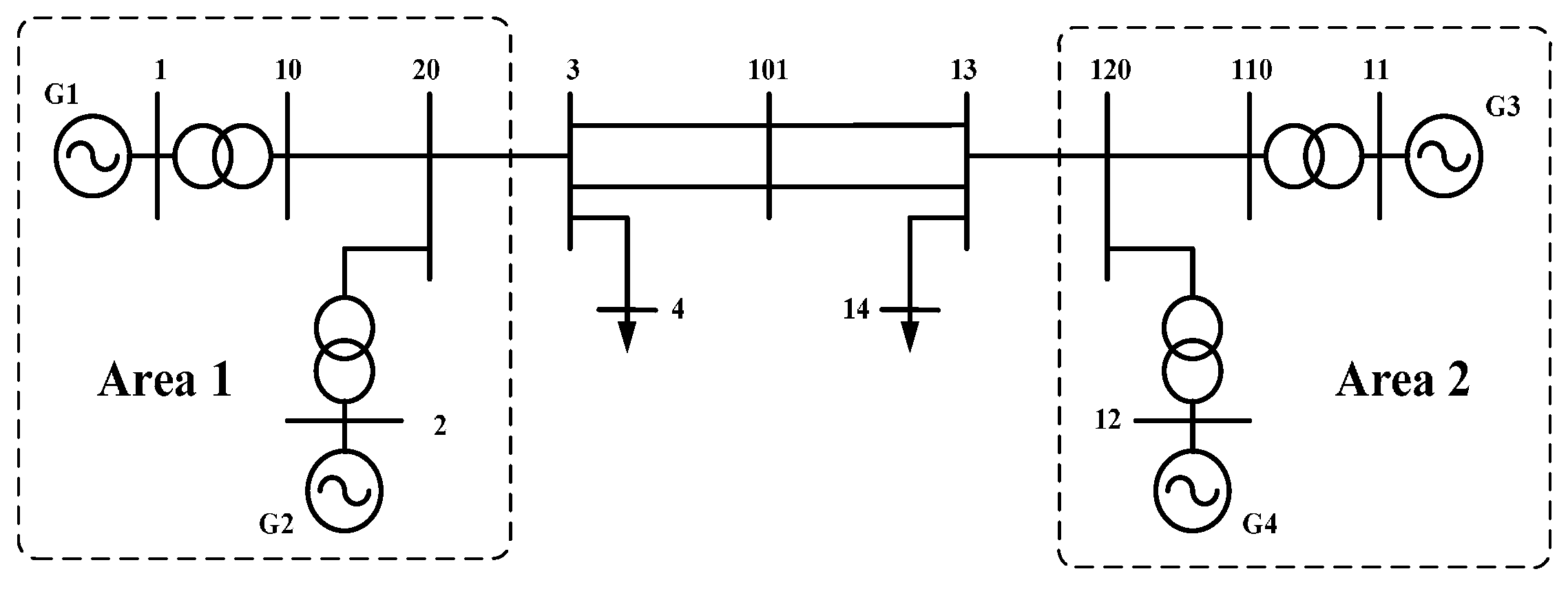
Figure 4.
Active power responses under different control schemes and cases: (a) The active power curve of tie-line under Case a; and (b) The active power curve of tie-line under Case b.
Figure 4.
Active power responses under different control schemes and cases: (a) The active power curve of tie-line under Case a; and (b) The active power curve of tie-line under Case b.
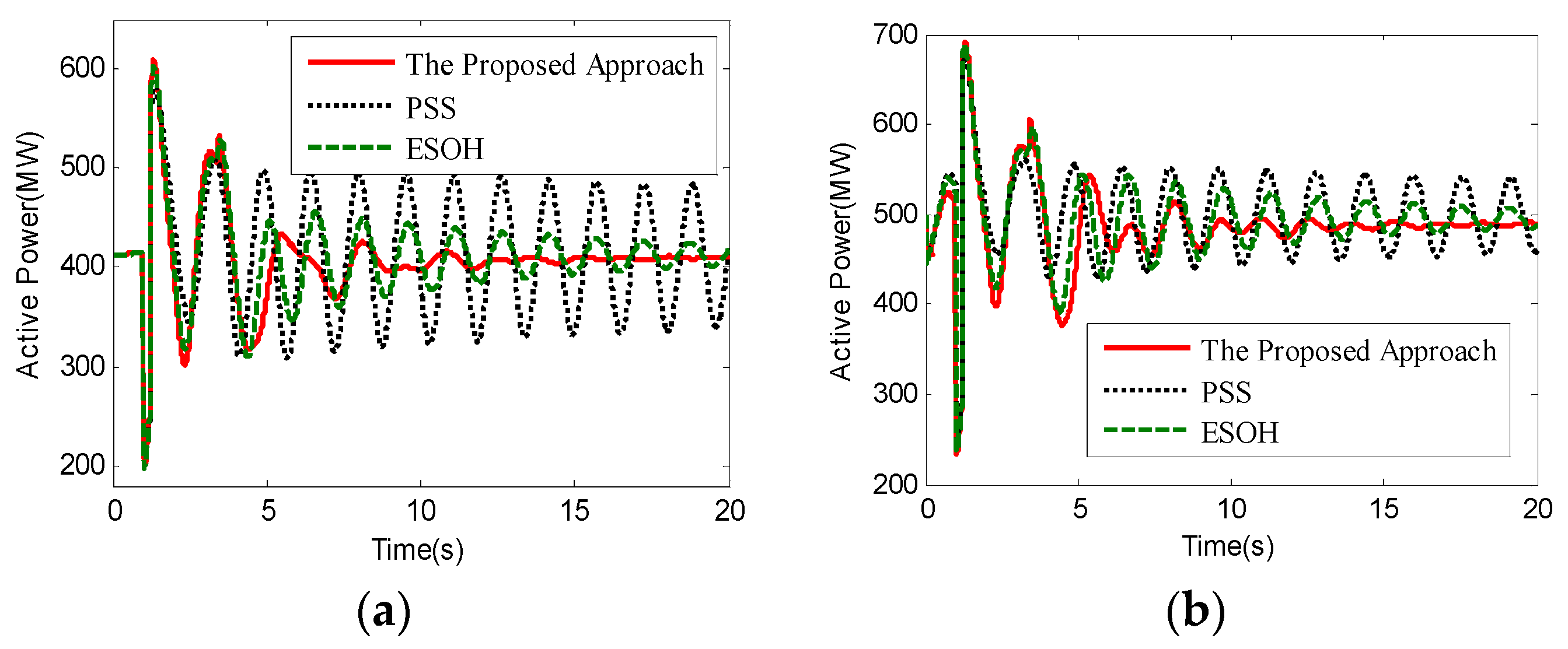
Figure 5.
System responses under different conditions and cases: (a) The active power curve of tie-line under different time delay periods; (b) The active power of G1 under noise; (c) Speed of G1 under parameters ε; and (d) The active power curve of tie-line under parameters T”d0.
Figure 5.
System responses under different conditions and cases: (a) The active power curve of tie-line under different time delay periods; (b) The active power of G1 under noise; (c) Speed of G1 under parameters ε; and (d) The active power curve of tie-line under parameters T”d0.
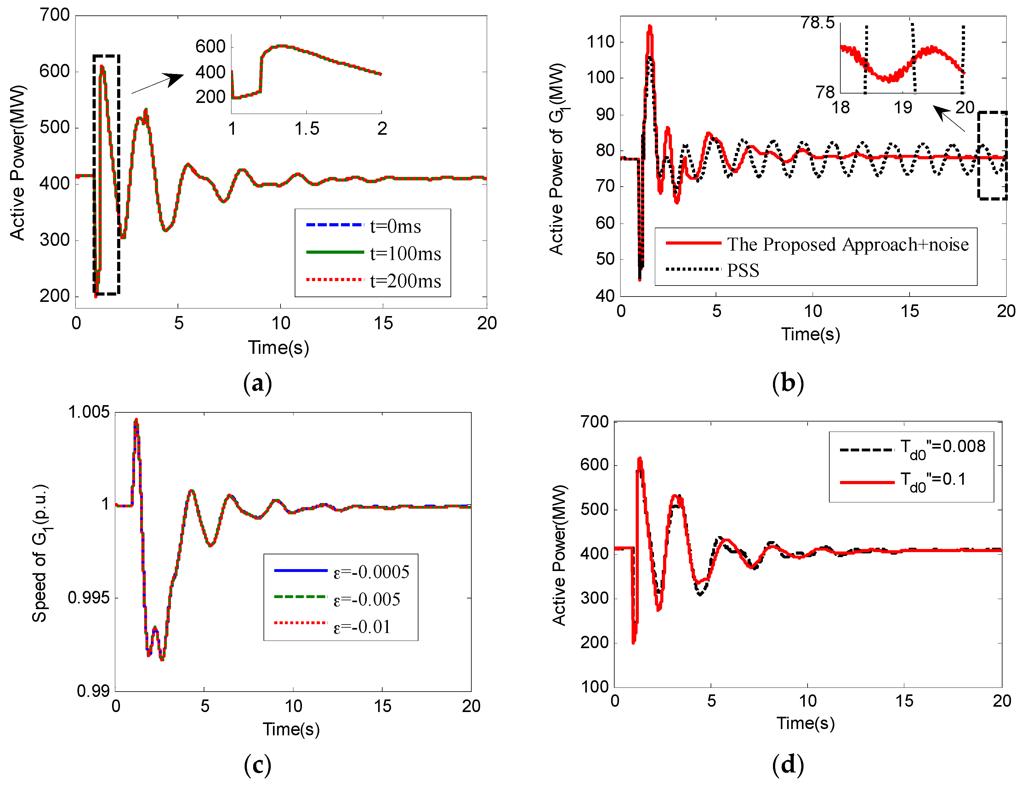
Figure 6.
Part of the Northeast network configuration.

Figure 7.
System responses under different control schemes and cases: (a) Active power of the DL line under Case a; and (b) Active power of the DL line under Case b.
Figure 7.
System responses under different control schemes and cases: (a) Active power of the DL line under Case a; and (b) Active power of the DL line under Case b.
Figure 8.
The simulation results. (a) Active power of the BW line under different time delay; (b) Active power of the SK line under parameters ε; (c) Active power of the SK line under system parameters variation; (d) Active power of the DL line under system parameters variation; and (e) Active power of the DL line under noise.


Table 1.
Identification results acquired by stochastic subspace identification (SSI). EBFSMC: ESO-BFSMC; ESOH: ESO-H∞; PSS: power system stabilizer.
Table 1.
Identification results acquired by stochastic subspace identification (SSI). EBFSMC: ESO-BFSMC; ESOH: ESO-H∞; PSS: power system stabilizer.
| Case | Inter-Area Oscillation Mode | Oscillation Generator Cluster | Control Scheme | |
|---|---|---|---|---|
| Frequency (Hz) | Damping (%) | |||
| a | 0.6439 | 0.24 | {1,2} vs. {3,4} | PSS |
| 0.6296 | 10.09 | {1,2} vs. {3,4} | ESOH | |
| 0.5256 | 13.15 | {1,2} vs. {3,4} | EFSMC | |
| b | 0.6228 | 1.77 | {1,2} vs. {3,4} | PSS |
| 0.6044 | 11.20 | {1,2} vs. {3,4} | ESOH | |
| 0.5975 | 11.91 | {1,2} vs. {3,4} | EFSMC | |
Table 2.
Identification results acquired by Prony method.
| Case | Input Signal | Critical Mode | |
|---|---|---|---|
| Frequency (Hz) | Damping (%) | ||
| a | wG13 | 0.64 | 0.08 |
| wG3 | 0.63 | 62.47 | |
| P3~13 a | 0.67 | 28.6 | |
| b | wG13 | 0.62 | 8.04 |
| wG3 | 0.59 | 74.05 | |
| P3~13 a | 0.69 | 64.99 | |
Table 3.
The related parameters of the controller design.
| Parameters | Value | Parameters | Value |
|---|---|---|---|
| T | 13 | Td0’ | 8 |
| xd | 1.8 | Tq0’ | 0.4 |
| xq | 1.7 | Td0” | 0.03 |
| xd’ | 0.3 | Tq0” | 0.05 |
| xq’ | 0.55 | Te | 0.001 |
| xd’’ | 0.25 | KA | 200 |
| xq’’ | 0.25 | Vref | 1.86756 |
Table 4.
Control parameters of the ESO regulator.
| Parameters | Value |
|---|---|
| β01 | 500,000 |
| α11 | 0.5 |
| δ1 | 0.001 |
| β02 | 3 |
| α21 | 0.25 |
| δ2 | 0.001 |
Table 5.
Control parameters of the FSMCB regulator.
| Parameters | Value |
|---|---|
| a1 | 0.001 |
| a2 | 100 |
| b1 | −0.0002 |
| b2 | 203.0667 |
| ε | −0.005 |
Table 6.
Control parameters of the ESOH regulator.
| Parameters | Value |
|---|---|
| p11 | −0.0002 |
| p21 | 43 |
Table 7.
Identification results acquired by SSI.
| Case | Inter-Area Oscillation Mode | Oscillation Generator Cluster | Control Scheme | |
|---|---|---|---|---|
| Frequency (Hz) | Damping (%) | |||
| a | 0.2514 | 27.47 | {ZDT, HMC, YKC, FSC, TLC} vs. {SZC, JJDZ} | PSS |
| 0.325 | 17.98 | {ZDT, HMC, YKC, FSC, TLC} vs. {SZC, JJDZ} | ESOH | |
| 0.2205 | 45.39 | {ZDT, HMC, FSC, YKC, TLC} vs. {SZC, JJDZ} | EFSMC | |
| b | 0.3053 | 9.79 | {ZDT} vs. {SZC, JJDZ, HMC, FSC, YKC, TLC, CYC} | PSS |
| 0.4294 | 15.01 | {ZDT} vs. {SZC, JJDZ, HMC, FSC, YKC, TLC, CYC} | ESOH | |
| 0.3403 | 20.28 | {ZDT} vs. {SZC, JJDZ, HMC, FSC, YKC, TLC, CYC} | EFSMC | |
Table 8.
The related parameters of the controller design.
| Parameters | Value | Parameters | Value |
|---|---|---|---|
| T | 5.5 | Td0’ | 5.837 |
| xd | 2.1553 | Tq0’ | 0.919 |
| xq | 2.1553 | Td0” | 0.045 |
| xd’ | 0.2647 | Tq0” | 0.069 |
| xq’ | 0.448 | Te | 0.01 |
| xd” | 0.2053 | KA | 500 |
| xq” | 0.212 | Vref | 5 |
Table 9.
Control parameters of the ESO regulator.
| Parameters | Value |
|---|---|
| β01 | 5000 |
| α11 | 0.5 |
| δ1 | 0.01 |
| β02 | –5 |
| α21 | 0.9 |
| δ2 | 0.01 |
Table 10.
Control parameters of the FSMCB regulator.
| Parameters | Value |
|---|---|
| a1 | –0.0000002 |
| a2 | –0.06 |
| b1 | –0.00002 |
| b2 | 1800 |
| ε | –0.5 |
© 2017 by the authors. Licensee MDPI, Basel, Switzerland. This article is an open access article distributed under the terms and conditions of the Creative Commons Attribution (CC BY) license (http://creativecommons.org/licenses/by/4.0/).
Share and Cite
MDPI and ACS Style
Liu, C.; Cai, G.; Gao, J.; Yang, D. Design of Nonlinear Robust Damping Controller for Power Oscillations Suppressing Based on Backstepping-Fractional Order Sliding Mode. Energies 2017, 10, 676. https://doi.org/10.3390/en10050676
AMA Style
Liu C, Cai G, Gao J, Yang D. Design of Nonlinear Robust Damping Controller for Power Oscillations Suppressing Based on Backstepping-Fractional Order Sliding Mode. Energies. 2017; 10(5):676. https://doi.org/10.3390/en10050676
Chicago/Turabian StyleLiu, Cheng, Guowei Cai, Jiwei Gao, and Deyou Yang. 2017. "Design of Nonlinear Robust Damping Controller for Power Oscillations Suppressing Based on Backstepping-Fractional Order Sliding Mode" Energies 10, no. 5: 676. https://doi.org/10.3390/en10050676
Note that from the first issue of 2016, this journal uses article numbers instead of page numbers. See further details here.