
A Low-Order System Frequency Response Model for DFIG Distributed Wind Power Generation Systems Based on Small Signal Analysis

1
College of Energy and Electrical Engineering, Hohai University, Nanjing 210098, China
2
Research Center for Renewable Energy Generation Engineering of Ministry of Eduction, Hohai University, Nanjing 210098, China
*
Author to whom correspondence should be addressed.
Energies 2017, 10(5), 657; https://doi.org/10.3390/en10050657
Submission received: 26 March 2017
/
Revised: 1 May 2017
/
Accepted: 2 May 2017
/
Published: 9 May 2017
Abstract
:Integrating large amounts of wind power into power systems brings a large influence on the dynamic frequency response characteristic (DFRC). The traditional low-order system frequency response (SFR) model is no longer applicable at the current time. Based on the small signal analysis theory, a set of novel low-order SFR models for doubly-fed induction generator (DFIG) distributed wind power generation systems (DWPGS) are derived under low, medium, and high wind speed conditions, respectively. Time-domain simulations have been conducted on PSCAD/EMTDC, and the novel SFR model is tested and evaluated on a real system. The simulation results from the novel model agree with those from the detailed model. The novel SFR model can also directly show the impact of the initial wind speed and auxiliary frequency controller (AFC) parameters on DFRC, but not on the detailed model.
1. Introduction
In the years 2014 and 2015, the Chinese Government Work Reports repeatedly addressed that sustainable energy production and an energy consumption revolution are beneficial to the improvement of people’s lives. China, along with many other developing countries in the world, has been challenged by growing air pollution issues and severe smoggy/hazy weather in the past decades. Therefore, it is increasingly necessary to move far forward in developing wind power energy and other clean energy worldwide. According to the 13th Five-Year Plan, Chinese installed wind energy capacity will reach at least two million kilowatts by 2020. However, due to the fact that most modern wind turbines equipped with power electronic converters, wind turbines’ rotor speeds are decoupled from the system dynamic frequency [1]. As a result, a large number of wind turbines integrated into traditional power system will change the system frequency dynamics. This is an urgent and important subject to study with respect to system frequency control strategies or system frequency response (SFR) models containing wind power.
At present, the majority of domestic and foreign literature basically focuses on enhancing the frequency response controlled by wind turbines. Ekanayake [2] had observed early on that there was a difference in dynamic response behaviors between doubly-fed induction generators (DFIG) and fixed-speed induction generators (FSIG) when the system frequency changes. DFIG is not capable of releasing the kinetic energy of their rotating mass, like FISG can, during frequency reduction. Morren et al. [3] proposed a method to allow variable speed wind turbines (VSWTs) emulate inertia and support primary frequency control by applying an additional proportional-differential (PD) controller loop. This has resulted in an embryonic form of frequency control techniques for VSWTs. Based on this, a large amount of research [4,5,6,7,8,9,10,11,12,13,14] has been conducted, which can generally be divided into three control modes: inertia control [4,5,6,7], primary frequency control [8,9,10,11,12], and combined inertia and primary frequency control [13,14]. However, the above research works are likely devoted to improving the frequency control ability of wind turbines themselves. In fact, the real frequency control ability of wind turbines contributing to the power system should be given more attention. However, so far, relatively little literature [15,16,17,18] focuses on the DFRC of power systems that include wind power generation. The quantitative analysis method of the impact on primary and secondary frequency control from wind power is shown in [15]. However, it is just a grid static frequency estimating method. We are still not capable of substantially mastering the DFRC. Fortunately, the research on DFRC for traditional power systems has been very mature [19,20,21]. A typical low-order SFR model for a traditional power system has been built in [19] by neglecting nonlinearities and all but the largest time constants in the equations of the power system.
Under the challenge of large wind power integration into power systems, the research on DFRC for distributed wind power systems has become an important subject to be solved. This paper mainly focuses on the DFIG distributed wind power generation systems (DWPGS). Firstly, the different simplified methods of the DFIG under low, medium, and high wind conditions have been analyzed according to their different response characteristics to the frequency disturbance. Secondly, based on the small signal analysis theory and the traditional SFR model, a novel SFR model has been deduced, and, further, can be used to analyze the impact of the initial operation point and parameters of auxiliary frequency controller (AFC) on DFRC directly. Finally, the novel SFR model is evaluated on a real DFIG DWPGS in Ontario, Canada.
2. Frequency Control Strategy and Response Characteristic of DFIG
The literature [8] proposed a set of frequency control strategies for all wind conditions. Among them are:
- (A)
- Low wind condition: As the available reserve capacity provided by the DFIG is very low, maintaining the DFIG in a stable condition is the first priority. In other words, the DFIG will provide no frequency control during system frequency fluctuations. Furthermore, due to the fact that the rotor speed of a DFIG is decoupled from the dynamic system frequency, DFIG could hardly release or absorb rotor kinetic energy, like the inertia response from synchronous generators. Hence, under low wind conditions, the extra active power provided from a DFIG is almost zero during a frequency disturbance.
- (B)
- Medium wind condition: In this wind region, DFIG can provide sufficient reserve capacity to participate in frequency control just by rotor over-speed regulation, and the pitch angle need not take an action (fixed at minimum angle ) just because the rotor speed could not exceed the upper limit . In order to make the novel SFR model derived in next section more representative, the original primary frequency control strategy in [8] is replaced by the combined inertia and primary control strategy [13,14,15,16,17] (shown in Figure 1) which is now more widely used. In addition, the reserve capacity command sent to the DFIG is set as a deloading rate d% [17] substituting for a fixed command . Once a frequency deviation happens in the system, the AFC will provide extra active power. Therefore, during the whole process of the frequency control, the output active power of DFIG can be expressed as:where, , represents the maximum power point tracking curve of DFIG in the medium wind region, and the deloading power point will deviate from the maximum power point by multiplying the deloading factor [17]. is the actual rotor speed, , is the air density, is the maximum wind power coefficient, is the optimal tip speed ratio, is the radius of wind blades, is the real-time frequency of power system, is the rated frequency, and , are the parameters of the AFC.As seen in Equation (1), it is important to note that the deloading power will be changed along with the actual rotor speed during the process of frequency control. More precisely, the changing amplitude is , but the key point is that the direction of the change is contrary to the extra active power provided by the AFC, causing an adverse effect on frequency control ability of the DFIG.
- (C)
- High wind condition: Above the rated wind speed, the DFIG should keep the torque and rotor speed less than the upper limit by pitch angle control. Therefore, unlike the medium wind condition, the output active power of the DFIG should be expressed as Equation (2) during the process of frequency control:where, is the rated torque, which is a constant value.
Obviously, the frequency response characteristic of the DFIG under low, medium, and high wind conditions are different from each other.
3. A Novel Low-Order SFR Model for DWPGS
This section is devoted to deriving a novel SFR model for DWPGS under low, medium, and high wind conditions, respectively. In order to present the core content clearly, it is necessary to make two reasonable assumptions: (I) the traditional power system shown in Figure 1 is dominated by a reheat-stream turbine [19]; and (II) the wind speed during the whole process of frequency response with a time scale of a minute is assumed constant.
According to small-signal eigenvalue analysis results of the detailed DFIG model in [22], it discovered that only the modal related to rotor speed plays a dominant role in system dynamic behaviors. The same conclusion is obtained in [4] based upon the eigenvalue sensitivity analysis. Therefore, from the point of system view, the simplified model of the DFIG can be represented as follows:
where, is the input mechanical power, is the output active power, is the inertia constant of the DFIG, and is the actual rotor speed of the DFIG.
3.1. Novel SFR Model under Low Wind Conditions
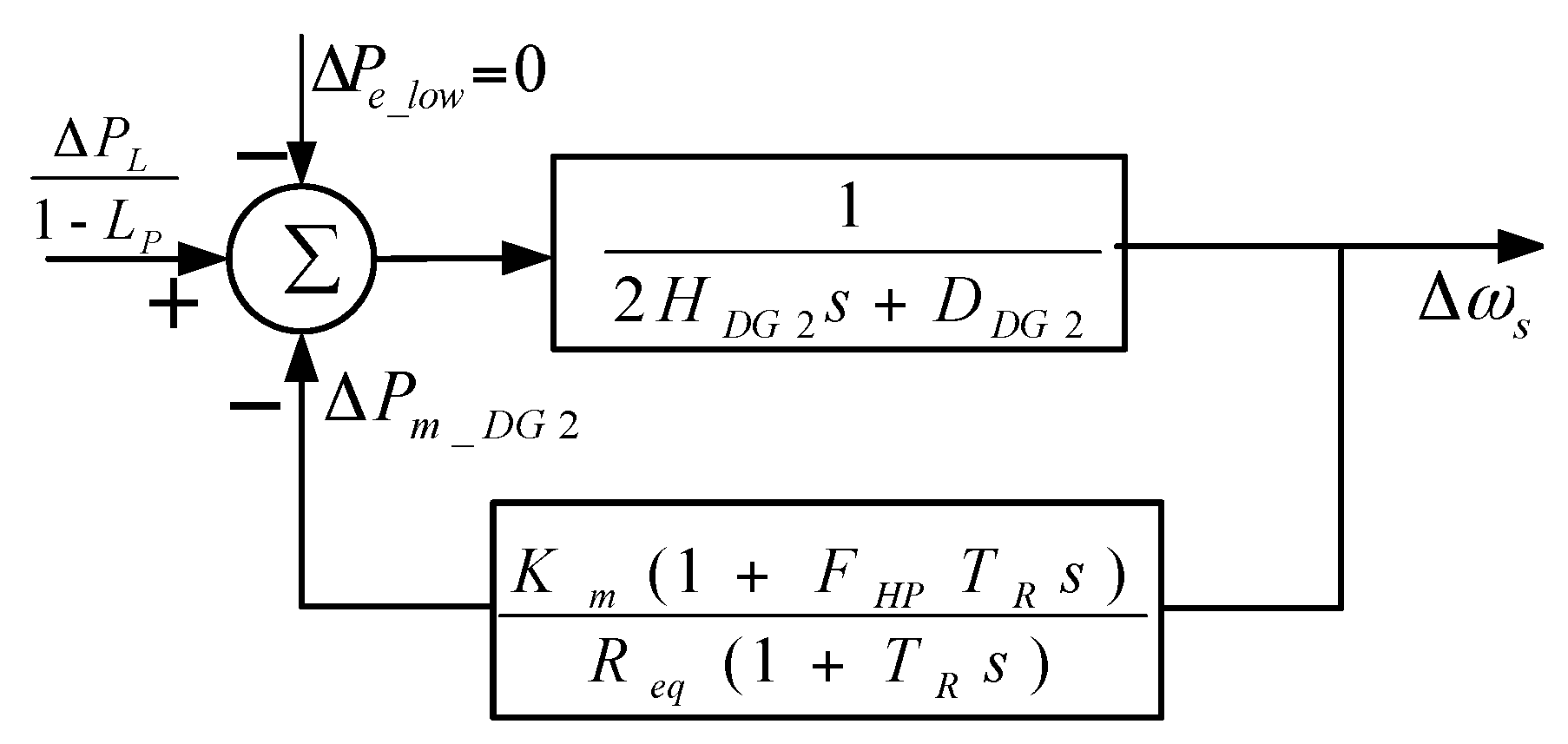
As previously stated, in low wind speed area, DFIG will not provide frequency control for the power system, but will protect itself in stable conditions as a first priority. It can be shown very easy from Equation (3) that the extra active power is zero just because the rotor speed is completely decoupled from the power system frequency . Thus, when percent of the reheat stream turbine unit capacity is replaced by DFIGs, the traditional SFR model [19] should be amended as the novel model shown in Figure 2. The only thing that needs to change is the active load disturbance (the original “” has been changed to because the real reheat stream turbine generator installed capacity has decreased times) and where, in Figure 2, , are the inertia constant and damping factor of the stream turbine, is the frequency deviation of the power system, is the permanent droop, is the mechanical power gain factor, is the fraction of total power generated by the HP turbine, and is the reheat time constant.
From the novel SFR model under low wind conditions shown in Figure 2, we can derive:
where , is the active load disturbance magnitude per unit based on the total installed capacity of the power system, and is the unit step function.
Based on the initial/final value theorem of the Laplace transform, the initial rate of change of frequency (IROCOF) and quasi-steady frequency deviation (QSFD) can be obtained:
Compared with the results from the traditional SFR model [19], it can be found that both the IROCOF and QSFD increase times after percent of the stream turbine capacity replaced by the DFIG with equal installed capacity. Thus, under the low wind condition, the frequency response ability of the power system would be weakened greatly.
3.2. Novel SFR Model under Medium Wind Conditions
When the wind rises to the medium wind region, the DFIG will provide frequency control for the power system just by its own rotor over-speed regulation (pitch angle is fixed at 0°). Thus, based on Equation (3), the simplified model of the DFIG during the process of frequency control can be specifically expressed as Equation (7):
where, , are the input mechanical power and output active power under medium wind conditions, respectively, is the expression of the wind power coefficient, , , (rated frequency, ), is the gear ratio, and is the number of pole pairs.
From the above simplified model of the DFIG (Equation (7)), a small-signal linear model can be developed as Equation (8) by selecting the state variable , output variable , and input variable , where :
and where , , , , , .
The transfer function between the input variable and the output variable can be derived by using the following conversion formula [23,24,25]:
Thus, the relationship between extra active power and power system frequency deviation can be represented as:
Based on Equation (10), when percent of the reheat stream turbine unit capacity is replaced by the DFIG, and the novel SFR model of the DFIG under medium speed conditions can be restructured (as seen in Figure 3). Among them, taking the real reheat stream turbine generator installed capacity as the datum, the extra output active power of the DFIG during frequency in per unit values can be expressed as . Meanwhile, the load disturbance occurring in the system turns out to be .
The novel SFR model depicted by Figure 3 can be effectively used to study how parameters kp and kd of the AFC and initial operation point affect the DFRC. The following subsections will discuss this in further detail.
3.2.1. Impact of the Initial Operating Point on System Frequency Dynamics Based on the Novel SFR Model
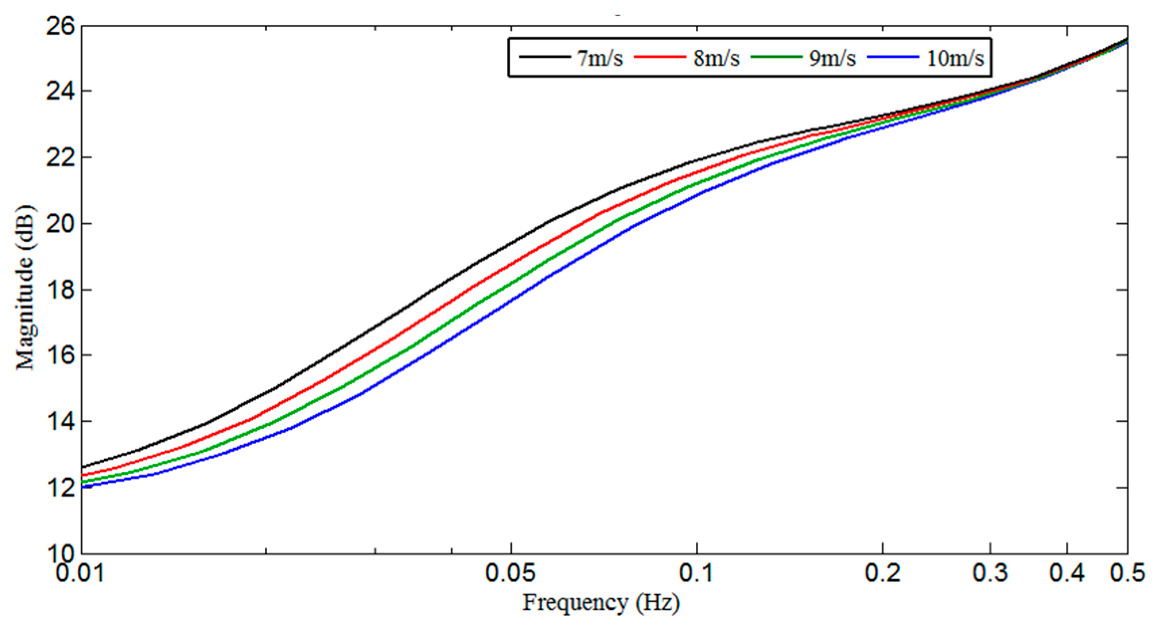
According to Equation (10), the initial rotor speed of the DFIG may directly affect the extra active power provided by the DFIG during a frequency disturbance. Meanwhile, the initial rotor speed is mainly dependent on the initial wind speed with the relationship , where, is the tip speed ratio under the over-speed-deloading running state [26]. Thus, the initial wind speed will have an influence on the frequency response of the DFIG and, in turn, on the system frequency dynamics. Figure 4 is the magnitude response (Bode diagram) which can reflect the relationship between and clearly. As shown, the lower initial wind speed, the larger extra the active power will be provided from the DFIG during the same frequency disturbance, and then the better the system frequency dynamic behaviors can be achieved. The main reason for this phenomenon is that a smaller change of deloading power will be obtained at lower initial wind speeds, which would cause a less adverse effect on the real frequency control ability of the DFIG under the same setting of parameters and .
3.2.2. Impact of Parameters of the AFC on System Frequency Dynamics Based on the Novel SFR Model
From Figure 3, the following transfer function can be obtained:
where, , , , , , , .
Thus, the initial rate of change of frequency (IROCOF) and the quasi-steady frequency deviation (QSFD) can be obtained:
As seen from Equations (12) and (13), it can be found that the parameter of the AFC has no inhibitory effect on IROCOF at all, but does have a positive effect on QSFD. On the contrary, the parameter has a direct inhibitory effect on IROCOF, however, it cannot improve the QSFD at all.
3.3. Novel SFR Model under High Wind Conditions
As mentioned previously, above the rated wind speed the DFIG cannot finish the deloading operation or frequency response control just by rotor over-speed control. Instead, a pitch controller will try to limit the rotor speed and the electromagnetic torque at the maximum allowable value . According to Equation (2), as well as the pitch angle control model [22], the detailed model of the DFIG under high wind conditions can be simplified as:
where is the constant time of the pitch angle servo, is an intermediate variable, and and are the PI controller parameters of the pitch angle.
By taking the state variables , input variables , and output variables , Equation (14) can be linearized as follows:
where , , , , , , .
Similarly, we can also figure out the relationship in the s-domain between and using Equation (9):
where .
Finally, the novel SFR model under high wind conditions can be developed, as shown in Figure 5, where, .
From Figure 5, the roughly consistent theoretical analysis results of the impact of the controller parameters and , with these under middle wind conditions, can be obtained:
4. Validation of the Novel Low-Order SFR Model
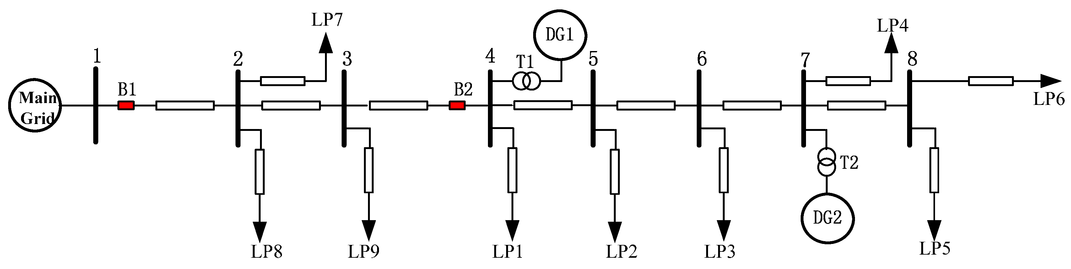
Up to now, the novel SFR models for the DFIG DWPGS from low wind conditions to high wind conditions are all derived. It is urgent, and also fascinating, to verify the novel SFR model. To do this, a real typical DFIG distribution system in Ontario, Canada (shown in Figure 6 [4]) is adopted. When the circuit breaker B2 is open, the segment after the breaker will work in isolated mode and the real system contains two distributed generation units DG1 and DG2, where DG1 is a DFIG, and DG2 is a traditional reheat stream turbine unit. The whole detailed model of the power system is built on PSCAD/EMTDC. The detailed DFIG model refers to [22,27], and the detailed reheat stream turbine containing a governor and excitation voltage regulator is adopted from the model library of PSCAD. System parameters are given in Appendix A.
4.1. Validation of the Novel SFR Model under Low Wind Condition
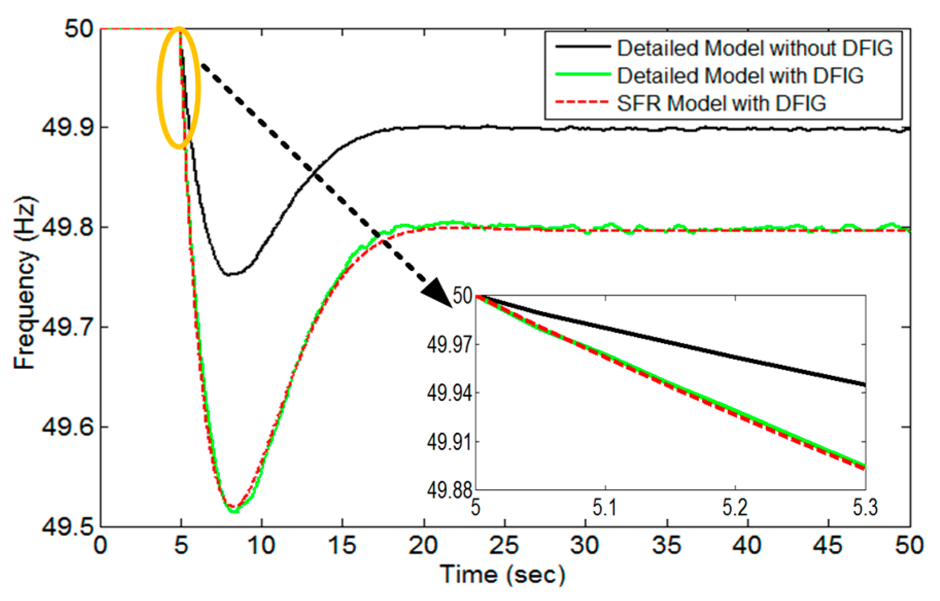
The simulation scenario is set as follows: The initial wind speed is 5 m/s, and the corresponding initial output power of the DFIG is 146.9 KW, which is relatively small and only accounts for about 6% of the rated power. For the balance of supply and demand, both LP1 and LP6 are disconnected from the power system in advance. When the simulation time arrives at 5 s, the whole 194.8 KW active power of LP6 switches into the system suddenly, causing a frequency disturbance in the power system. As the DFIG cannot provide frequency control just for its own stability under this condition. The frequency response dynamic curves obtained from the proposed SFR model and the detailed model are compared in Figure 7.
As seen from Figure 7, the novel SFR has been validated in two aspects: (a) intuitively, the curves of the frequency obtained from detailed model and SFR model containing the DFIG are in good agreement; and (b) before the 2.5 MW DFIG (DG1, 50% of total installed capacity) displaces the equal capacity of a traditional reheat stream turbine (DG2), the IROCOF and QSFD of the power system are 0.194 Hz/s and −0.1020 Hz, respectively. Then, the IROCOF and QSFD change to 0.388 Hz/s and −0.2041 Hz, accordingly, which is two times larger than the former after DG1 was substituted into the system. These results prove the theoretical derivations of Equations (5) and (6) to be correct.
4.2. Validation of the Novel SFR Model under Medium Wind Conditions
4.2.1. Validation of the Accuracy of the Novel SFR Model by Comparison with the Detailed Model
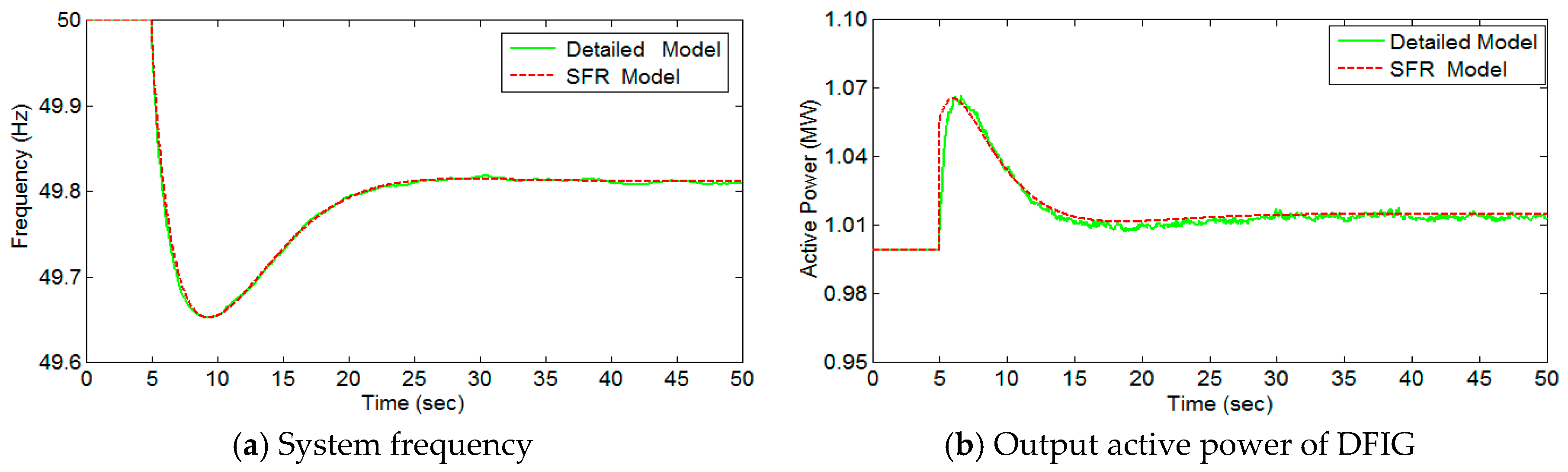
The typical medium wind speed 9 m/s is chosen as the initial current wind speed, and the DFIG is deloaded by 10% in advance so as to provide sufficient reserve capacity for frequency control. At this point, the initial output active power of the DFIG is 998 KW, hence, LP5 and LP6 are switched off for load balancing between supply and demand. The same load disturbance as in the previous simulation is adopted, and the parameters and of the AFC are set at 16 and 10, respectively. Finally, the system frequency of the output active power of the DFIG based on the novel SFR model and the detailed model are depicted and compared in Figure 8.
As shown in Figure 8a,b, when the load disturbance happens at 5 s, the dynamic behaviors of the system frequency and output active power of the DFIG based on the SFR model are accurately simulated by comparing with the detailed model. In other words, the novel SFR model can represent the dynamic frequency response behaviors for the DFIG DWPGS.
4.2.2. Validation of the Impact of the Initial Operation Point on the DFRC
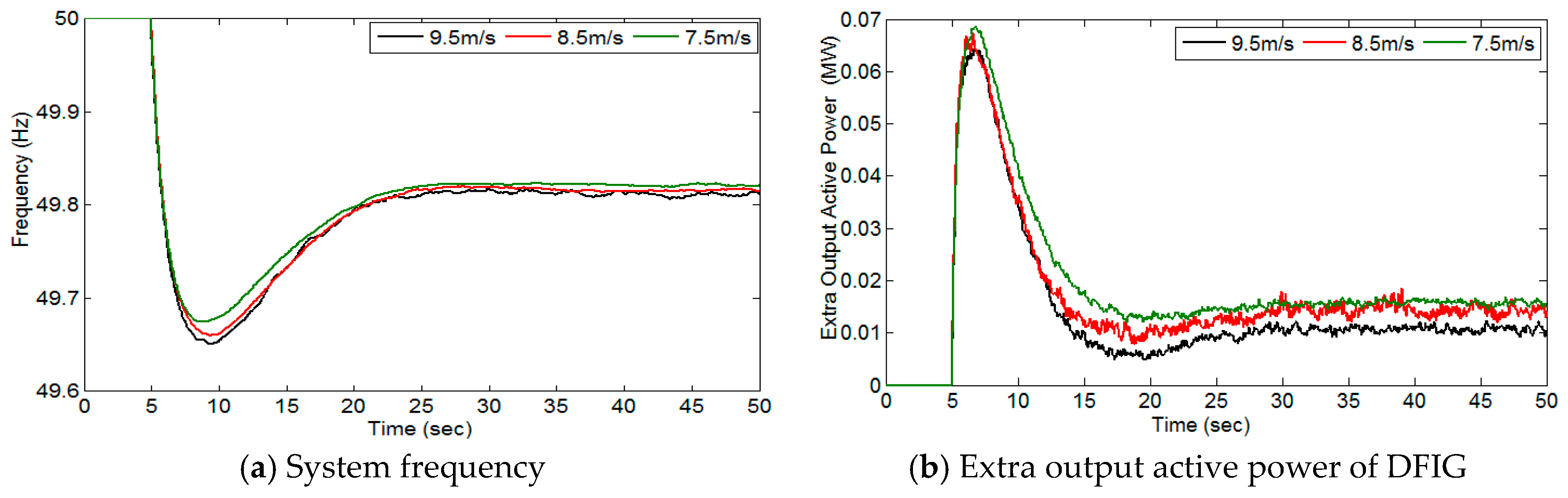
The simulation tests for the validation of the impact of the initial operation are conducted in this subsection. The parameters and kd are still set at 16 and 10, respectively, and three typical medium wind speeds of 9.5 m/s, 8.5 m/s, and 7.5 m/s are selected as the initial wind speeds, successively. The different dynamic frequency response behaviors are obtained and compared in Figure 9.
From Figure 9a, it is clear to see that the DFRC can perform better under a lower initial wind speed during the same load disturbance event. Figure 9b further explains the reason is that the DFIG can provide more extra active power to support system frequency recovery, which has been clearly and directly analyzed in Section 3.2.1 based on the novel SFR model.
4.2.3. Validation of the Impact of the Control Parameters , of the AFC on the DFRC
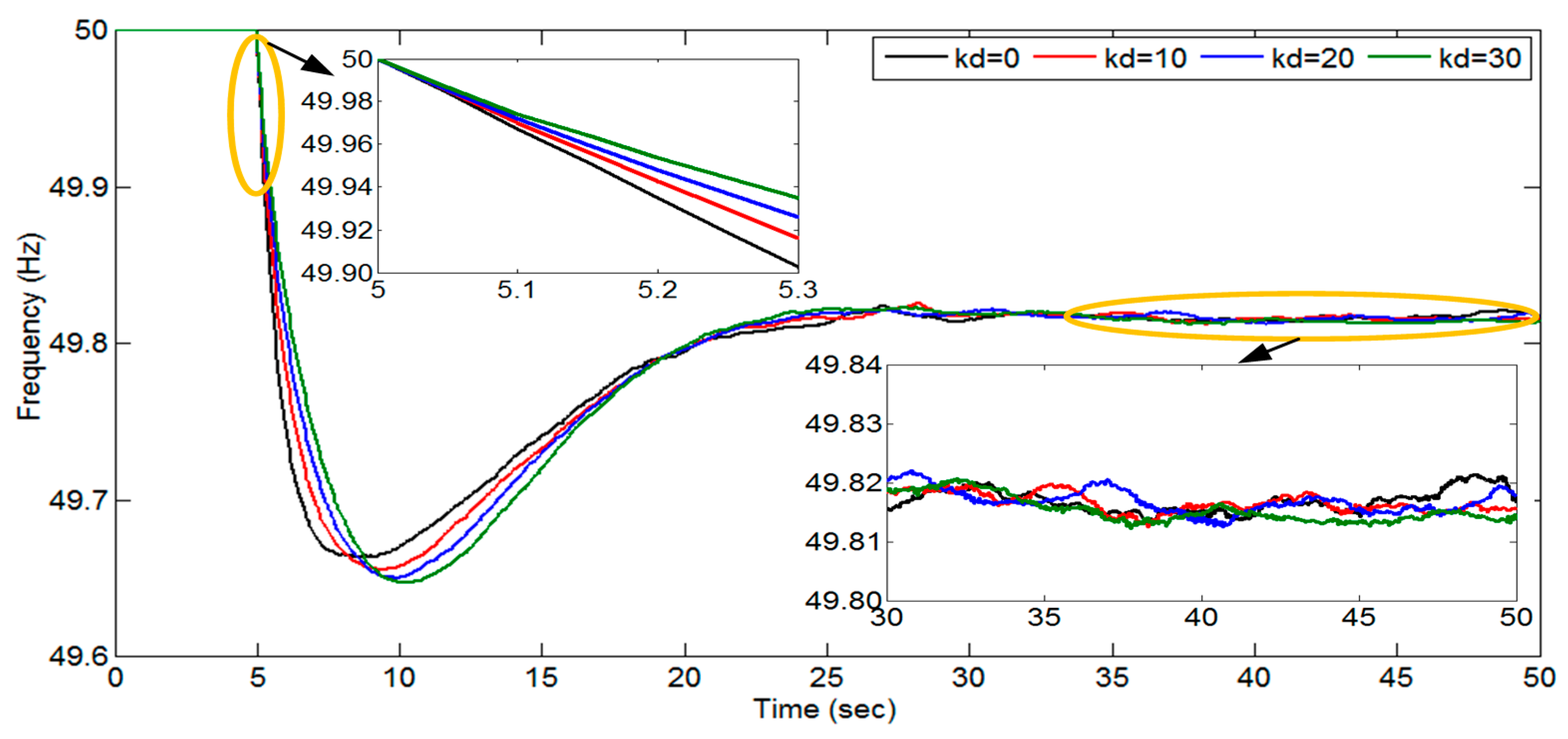
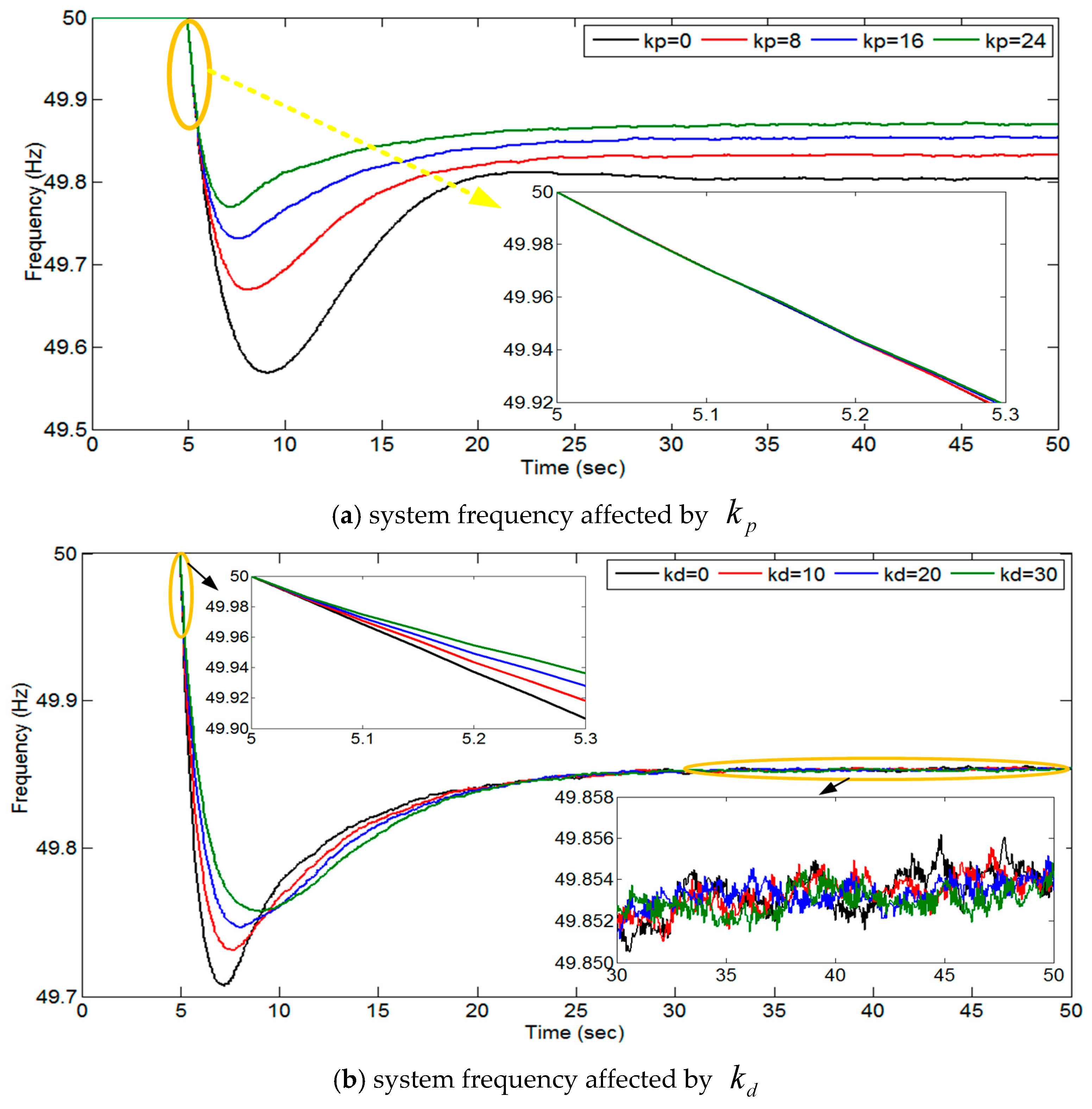
According to the derivative results from the novel SFR model in Section 3.2.2, it is suggested that the control parameter has a positive effect on QSFD, but does not have any inhibitory effect on IROCOF, yet, for , it is the contrary. To confirm the analysis results, two different cases are designed for the detailed model: CASE I: increase (0, 8, 16, 24) successively, meanwhile keeping constant; and CASE II: increase (0, 10, 20, 30) in turn, and keep unchanged. The simulation results under CASE I and CASE II are shown in Figure 10 and Figure 11, respectively.
As shown in Figure 10, two main simulation results can be observed: (1) with an increase of parameter (0, 8, 16, 24), the frequency response curves coincide with each other at the initial stage (5.1–5.3 s). This means that IROCOF is insensitive to the change of parameter at all. That is, has no inhibitory effect on IROCOF; (2) meanwhile, an increase in improves the frequency dynamics, which can be mainly reflected by two dynamic indices: maximum frequency deviation (MFD) and QSFD. Instead, as depicted in Figure 11, it is easy to notice a decrease of IROCOF with the increase of , but an increase of MFD can also be observed. This is mainly because a higher setting will result in a larger rotor kinetic energy release at the beginning of the frequency drop. However, it also results in a larger change of deloading power , which causes a more notable adverse effect on the MFD, correspondingly. Meanwhile, as the rate of the frequency change decreases rapidly during frequency recovery, parameter becomes insensitive to the frequency change. As expected, no matter how the changes, QSFD basically stays around the −0.184 Hz level.
4.3. Validation of the Novel SFR Model under High Wind Conditions
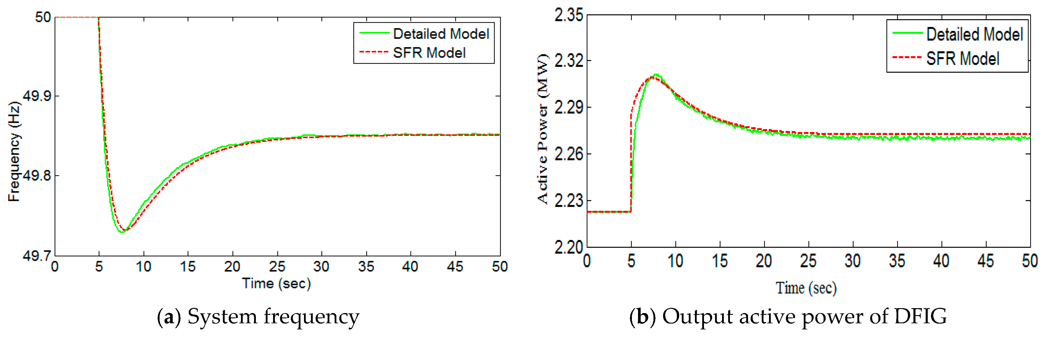
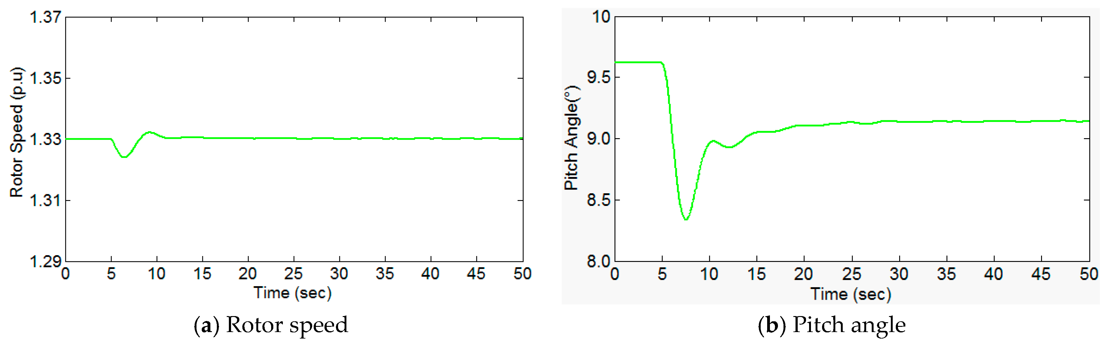
The novel SFR for the DFIG DWPGS above rated wind speeds is tested in this section. It is assumed that the current wind speed reaches 13 m/s, and DFIG is also deloaded by 10%. All loads, except LP6, access the power system at the beginning of the simulation. The same load disturbance happens at 5 s. Finally, the comparative results between the detailed model and the novel SFR model under high wind conditions are shown in Figure 12.
As depicted in Figure 12a,b, the curve of the dynamic system frequency and the output active power of the DFIG simulated from the novel SFR model under high wind conditions agree well with those from the detailed model. That is, under the high wind condition, the simplified model of the DFIG, as expressed in Equation (14), can represent the dynamic behavior of the frequency of the DFIG correctly. Further, seen in the Figure A1 in Appendix B, it is clear to show that the whole process of the DFIG frequency response is mainly controlled by the pitch angle, whereas the rotor speed is limited by the maximum allowable value . In addition, the impact of controller parameters , under high wind conditions can be verified effectively by basically the same simulation, which are verified in Figure 13. The only difference is that the initial deloading power remains nearly constant during the process of frequency response under high wind conditions. Therefore, the adverse effect on MFD with the increase of could not exist anymore. Additionally, the initial operation point would have little impact on the DFRC under high wind conditions.
5. Conclusions
Since the DFIG responds differently to frequency disturbances under low, medium, and high wind conditions, the authors proposed a complete set of novel SFR models for DFIG DWPGS developed from the simplified small-signal analysis theory. Compared with the detailed model, this novel model not only makes it more convenient to obtain the frequency dynamic curves containing the important dynamic frequency indexes, but also provides a more clear and direct way to understand the impact of the initial operating point and parameters of the AFC on DFRC. Moreover, it should be pointed out that the novel SFR model is applicable to all DFIG DWPGS except at extreme conditions, in which the DFIG responds excessively and loses stability by oversizing the parameters and of the AFC [10]. It is worthwhile to look to the future when more complicated SFR models for large-scale wind grid-connect power systems may be constructed based on the novel SFR model presented in this paper.
Acknowledgments
This work was supported in part by the National Nature Science Foundation of China (No. 5137704) and the Funding of the Jiangsu Innovation Program for Graduate Education (No. CXLX13_226).
Author Contributions
Rui Quan and Wenxia Pan conceived and designed the study; Rui Quan designed and performed the simulations; Rui Quan and Wenxia Pan wrote the paper. Wenxia Pan provides a lot of useful guidances and constructive suggestions in later the improvement of the revised manuscript. All authors revised and approved the publication.
Conflicts of Interest
The authors declare no conflict of interest.
Appendix A
DFIG physical parameters:
HDG1 = 3.64 s, Cpmax = 0.4382, R = 43.25 m, , Prate_DG1 = 2.5 MW, = 1.2 p.u, ωrmax = 1.33 p.u, = 11.6 m/s, p = 3, , , .
Traditional Power System Parameters:
HDG2 = 5 s, DDG2 = 0.1, TR = 12 s, Req = 0.05, FHP = 0.3, Km = 0.95, LP1: 47 KW + j15.61 KVAR, LP2: 2565 KW + j843.06 KVAR, LP3: 289.75 KW + j95.24 KVAR, LP4: 152 KW + j49.96 KVAR, LP5: 517.8 KW + 170.18 KVAR, LP6: 194.8 KW + j64.01 KVAR.
Appendix B
Figure A1.
The dynamic response curve of DFIG under high wind condition VW = 13 m/s.

References
- He, C.M.; Wang, H.T. Coordination frequency control strategy design of wind farm base on time sequence control. In Proceedings of the IEEE PES Asia-Pacific Power and Energy Engineering Conference, Beijing, China, 8–11 December 2013; pp. 1–6. [Google Scholar]
- Ekanayake, J.; Jenkins, N. Comparison of the response of doubly fed and fixed-speed induction generator wind turbines to changes in network frequency. IEEE Trans. Power Syst. 2004, 19, 800–802. [Google Scholar] [CrossRef]
- Morren, J.; de Haan, S.W.H.; Kling, W.L.; Ferreira, J.A. Wind turbines emulating inertia and supporting primary frequency control. IEEE Trans. Power Syst. 2006, 21, 433–434. [Google Scholar] [CrossRef]
- Arani, M.F.M.; EI-Saadany, E.F. Implementing Virtual Inertia in DFIG-Based Wind Power Generation. IEEE Trans. Power Syst. 2013, 28, 1373–1384. [Google Scholar] [CrossRef]
- Papadimitriou, C.N.; Vovos, N.A. Transient Response Improvement of Micro-grids Exploiting the Inertia of a Doubly-Fed Induction Generator (DFIG). Energies 2010, 3, 1049–1066. [Google Scholar] [CrossRef]
- Licari, J.; Ekanayake, J.; Moore, I. Inertia response from full-power converter-based permanent magnet wind generators. J. Mod. Power Syst. Clean Energy 2013, 1, 26–33. [Google Scholar] [CrossRef]
- Keung, P.K.; Li, P.; Banakar, H.; Ooi, B.T. Kinetic energy of wind turbine generators for system frequency support. IEEE Trans. Power Syst. 2009, 24, 279–287. [Google Scholar] [CrossRef]
- Chang-Chien, L.R.; Lin, W.T.; Yin, C.Y. Enhancing frequency response control by DFIGs in the high wind penetrated power systems. IEEE Trans. Power Syst. 2011, 26, 710–718. [Google Scholar] [CrossRef]
- Vidyanandan, K.V.; Senroy, N. Primary frequency regulation by deloaded wind turbines using variable droop. IEEE Trans. Power Syst. 2013, 28, 837–846. [Google Scholar] [CrossRef]
- Pan, W.X.; Quan, R.; Wang, F.A. Variable droop control strategy for doubly-fed induction generators. DianliXitong Zidonghua 2015, 39, 126–131. [Google Scholar]
- Ullah, N.R.; Thiringer, T.; Karlssom, D. Temporary primary frequency control support by variable speed wind turbines-potential and applications. IEEE Trans. Power Syst. 2008, 23, 601–602. [Google Scholar] [CrossRef]
- De-Almeida, R.G.; Pecas-Lopes, J.A. Participation of doubly fed induction wind generators in system frequency regulation. IEEE Trans. Power Syst. 2007, 22, 944–950. [Google Scholar] [CrossRef]
- Ma, H.T.; Chowdhury, B.H. Working towards frequency regulation with wind plants: Combined control approaches. IET Renew. Power Gener. 2010, 4, 308–316. [Google Scholar] [CrossRef]
- Ghosh, S.; Kamalasadan, S.; Senroy, N. Doubly fed induction generator (DFIG)-based wind farm control framework for primary frequency and inertia response application. IEEE Trans. Power Syst. 2016, 31, 1861–1871. [Google Scholar] [CrossRef]
- Ding, L.; Qiao, Y.; Lu, Z.X. Impact on frequency regulation of power system from wind power system with high penetration. DianliXitong Zidonghua 2014, 38, 1–8. [Google Scholar]
- Wang, Y.; Deille, G.; Bayem, H. High wind power penetration in isolated power system—Assessment of wind inertia and primary frequency response. IEEE Trans. Power Syst. 2013, 28, 2412–2420. [Google Scholar] [CrossRef]
- Pradhan, C.; Bhene, C.N. Frequency sensitivity analysis of load damping co-efficient in wind farm-integrated power system. IEEE Trans. Power Syst. 2017, 32, 1016–1029. [Google Scholar]
- Doherty, R.; Mullane, A.; Nolan, G. An assessment of the impact of wind generation on system frequency control. IEEE Trans. Power Syst. 2010, 25, 452–460. [Google Scholar] [CrossRef]
- Anderson, P.M.; Mirheydar, M. A low-order system frequency response model. IEEE Trans. Power Syst. 1990, 5, 720–729. [Google Scholar] [CrossRef]
- Anderson, P.M.; Mirheydar, M. An adaptive method for setting under frequency load shedding relays. IEEE Trans. Power Syst. 1992, 7, 647–655. [Google Scholar] [CrossRef]
- Aik, D.L.H. A general-order system frequency response model incorporating load shedding: Analytic modeling and application. IEEE Trans. Power Syst. 2006, 21, 709–717. [Google Scholar] [CrossRef]
- Lin, J.; Li, G.J.; Sun, Y.Z.; Li, X. Small-signal analysis and control system parameter optimization for DFIG wind turbines. DianliXitong Zidonghua 2009, 33, 86–90. [Google Scholar]
- Ragavan, K.; Satish, L. An efficient method to compute transfer function of a transformer from its equivalent circuit. IEEE Trans. Power Deliv. 2005, 20, 780–788. [Google Scholar] [CrossRef]
- Liu, W.Y.; Ge, R.D.; Lv, Q.C.; Li, H.Y.; Ge, J.B. Research on a small signal stability region boundary model of the interconnected power system with large-scale wind power. Energies 2015, 8, 2312–2336. [Google Scholar] [CrossRef]
- Kundur, P. Power System Stability and Control; McGraw-Hill Professional: New York, NY, USA, 1994; pp. 792–804. [Google Scholar]
- Zhang, Z.S.; Sun, Y.Z.; Li, G.J.; Cheng, L.; Lin, J. Frequency regulation by doubly fed induction generator wind turbines based on coordinated over-speed control and pitch control. DianliXitong Zidonghua 2011, 35, 20–25. [Google Scholar]
- Wu, F.; Zhang, X.P.; Godfrey, K. Small signal stability analysis and optimal control of a wind turbine with doubly fed induction generator. IET Gener. Trans. Distrib. 2007, 1, 751–760. [Google Scholar] [CrossRef]
Figure 1.
The detailed model structure of DFIG distributed wind power systems.
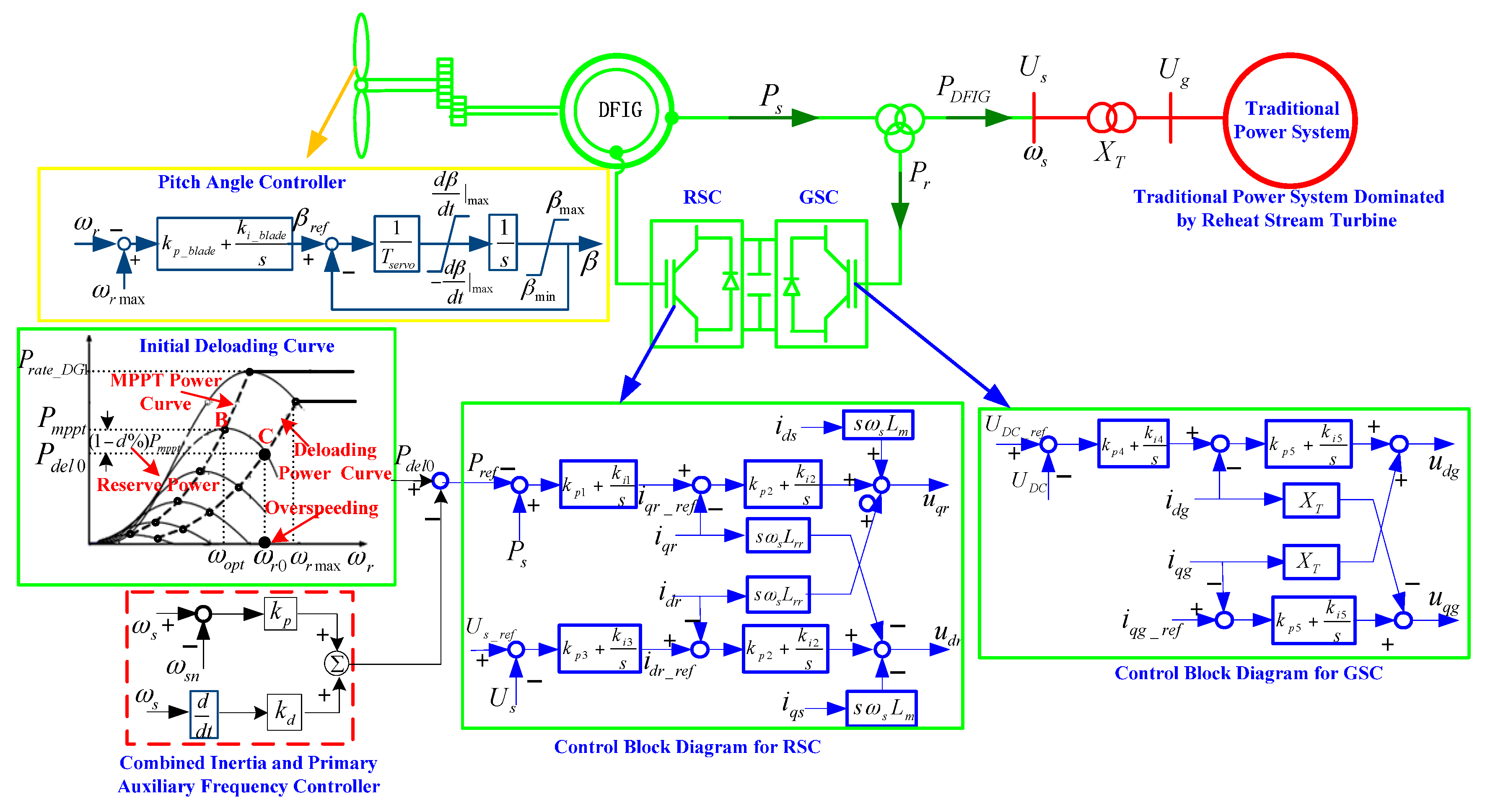
Figure 2.
The novel SFR model under low wind condition.

Figure 3.
The novel SFR model under medium wind conditions.
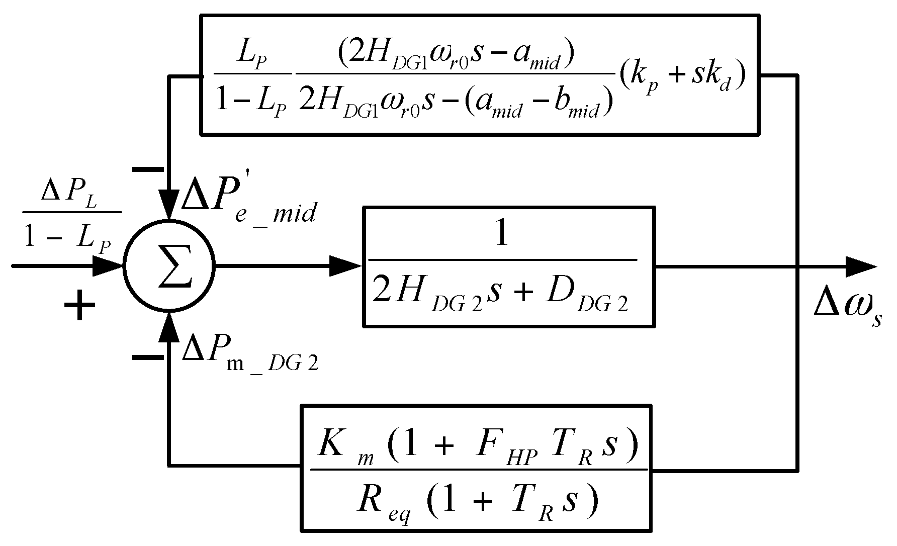
Figure 4.
The impact of initial wind speed on the magnitude response of the DFIG extra output power during frequency control.
Figure 4.
The impact of initial wind speed on the magnitude response of the DFIG extra output power during frequency control.

Figure 5.
The novel SFR model under high wind conditions.
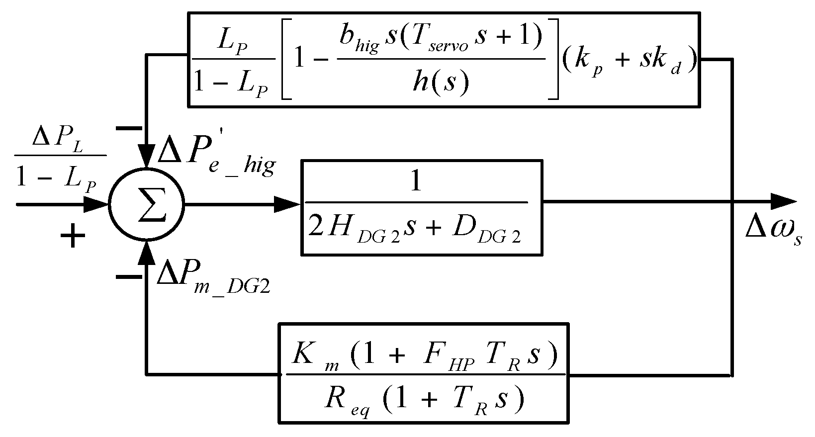
Figure 6.
A real DFIG distributed rural system in Ontario, Canada.

Figure 7.
Comparisons of frequency response dynamics between the detailed model and the novel SFR model under low wind condition (note: “without or with DFIG” means a traditional power system with a total installed capacity of 5 MW is not displaced, or is displaced partly, by the DFIG with a rated capacity of 2.5 MW).

Figure 8.
Comparisons of the frequency response dynamics between the detailed model and the novel SFR model under medium wind conditions.
Figure 8.
Comparisons of the frequency response dynamics between the detailed model and the novel SFR model under medium wind conditions.

Figure 9.
The impact of the initial operating point on the frequency response dynamics based on the detailed model.
Figure 9.
The impact of the initial operating point on the frequency response dynamics based on the detailed model.

Figure 10.
The impact of parameter on the frequency response dynamics based on the detailed model (CASE I).
Figure 10.
The impact of parameter on the frequency response dynamics based on the detailed model (CASE I).
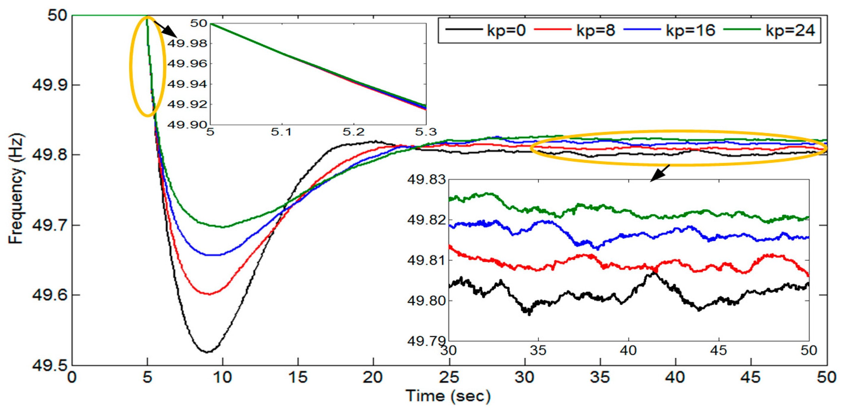
Figure 11.
The impact of parameter on the frequency response dynamics based on the detailed model (CASE II).
Figure 11.
The impact of parameter on the frequency response dynamics based on the detailed model (CASE II).

Figure 12.
Comparisons of the frequency response dynamics between the detailed model and novel SFR model under high wind conditions.
Figure 12.
Comparisons of the frequency response dynamics between the detailed model and novel SFR model under high wind conditions.

Figure 13.
The impact of the parameters of the AFC on the frequency response dynamics under high wind conditions.
Figure 13.
The impact of the parameters of the AFC on the frequency response dynamics under high wind conditions.
© 2017 by the authors. Licensee MDPI, Basel, Switzerland. This article is an open access article distributed under the terms and conditions of the Creative Commons Attribution (CC BY) license (http://creativecommons.org/licenses/by/4.0/).
Share and Cite
MDPI and ACS Style
Quan, R.; Pan, W. A Low-Order System Frequency Response Model for DFIG Distributed Wind Power Generation Systems Based on Small Signal Analysis. Energies 2017, 10, 657. https://doi.org/10.3390/en10050657
AMA Style
Quan R, Pan W. A Low-Order System Frequency Response Model for DFIG Distributed Wind Power Generation Systems Based on Small Signal Analysis. Energies. 2017; 10(5):657. https://doi.org/10.3390/en10050657
Chicago/Turabian StyleQuan, Rui, and Wenxia Pan. 2017. "A Low-Order System Frequency Response Model for DFIG Distributed Wind Power Generation Systems Based on Small Signal Analysis" Energies 10, no. 5: 657. https://doi.org/10.3390/en10050657
Note that from the first issue of 2016, this journal uses article numbers instead of page numbers. See further details here.