
Identification of Non-Stationary Magnetic Field Sources Using the Matching Pursuit Method

Department of Marine Telecommunications, Gdynia Maritime University, Morska 81-87, 81-225 Gdynia, Poland
Energies 2017, 10(5), 655; https://doi.org/10.3390/en10050655
Submission received: 16 February 2017
/
Revised: 23 April 2017
/
Accepted: 4 May 2017
/
Published: 9 May 2017
(This article belongs to the Special Issue Selected Papers from 16 IEEE International Conference on Environment and Electrical Engineering (EEEIC 2016))
Abstract
:The measurements of electromagnetic field emissions, performed on board a vessel have showed that, in this specific environment, a high level of non-stationary magnetic fields (MFs) is observed. The adaptive time-frequency method can be used successfully to analyze this type of measured signal. It allows one to specify the time interval in which the individual frequency components of the signal occur. In this paper, the method of identification of non-stationary MF sources based on the matching pursuit (MP) algorithm is presented. It consists of the decomposition of an examined time-waveform into the linear expansion of chirplet atoms and the analysis of the matrix of their parameters. The main feature of the proposed method is the modification of the chirplet’s matrix in a way that atoms, whose normalized energies are lower than a certain threshold, will be rejected. On the time-frequency planes of the spectrograms, obtained separately for each remaining chirlpet, it can clearly identify the time-frequency structures appearing in the examined signal. The choice of a threshold defines the computing speed and precision of the performed analysis. The method was implemented in the virtual application and used for processing real data, obtained from measurements of time-vary MF emissions onboard a ship.
1. Introduction
The aim of the research of a non-stationary magnetic field (MF) is to improve the tools for the analysis of low-frequency MF emissions in a ship’s environment considering the limits for MF exposures, which are defined by International Commission on Non-Ionizing Radiation Protection (ICNIRP) [1]. The requirements for protection against multi-frequency steady-state MF emissions are determined by the formula indicated in ICNIRP guidelines. Instantaneous values of this summation formula can be estimated with a joint time-frequency-domain method of analyzing of the digitized magnetic-flux density time series acquired by measurement. The problem of the high MF emissions is important because the exposure to the MF may have biological effects, depending on the frequency range of fields, intensity of emissions, and conditions of exposure. The standard documents, both in the scope of the electromagnetic compatibility of technical equipment and in limiting human exposure to MF emissions, define the admissible limits of magnetic-field intensities [1,2]. The effective methods of reduction of the undesirable emissions require the identification of the MF sources within the examined environment. The results of MF measurements performed on board of the Gdynia Maritime University research-training vessel during maneuvering and sea voyages indicate the places with a high level of MF emissions [3]. The MF spectrum spreads out mostly in the low-frequency range, below 2 kHz. The measured signals, representing MF induction waveforms consist of time-varying harmonics, in which magnitude, frequency and phase fluctuate over time. This type of signal has an evolutionary spectrum and can also include time-varying broadband spectral components. In order to analyze the non-stationary signal in time periods and its spectrum distribution, time-frequency methods can be used. Currently, many researchers of different fields use the adaptive time-frequency representation of signals to separate local structures of the signal and assess their characteristics [4,5,6,7,8,9,10,11,12]. The joint time-frequency methods allow the indication of a high time resolution some time periods, where the examined signal constituents of different frequencies appear. The measured waveforms corresponding to the sources of high-level MFs usually concentrate in a relatively narrow frequency band. After conversion to the joint time-frequency domain the dominant structures of the analyzed signal can be distinguished in a time-frequency plane. This way, the MF sources are identifiable in the tested environment. The presented paper proposes the method of the recognition of the low-frequency MF sources. The adaptive analysis, based on a matching pursuit (MP) procedure is applied. The MP approximation algorithm was introduced by Mallat and Zhang [13] and Qian and Chen [14] at the beginning of the 1990s. It is a kind of iterative algorithm, which decomposes any signal into a linear combination of elementary functions, called atoms, chosen within an over-complete dictionary in order to best match the signal structures [15,16,17,18]. The bigger (more redundant) this dictionary is, the better the chance of finding a more accurate signal expansion. The choice of a type of atoms in a time-frequency dictionary is of extreme importance, since its features should ideally match the properties of the analyzed signals. The chirp functions with Gaussian envelopes (chirplets) effectively describe measured waveforms corresponding to a time-varying MF induction [18]. The next significant matter is the fixing of the optimal number of steps in the MP algorithm. The excessive number of elementary functions in the signal representation does not noticeably improve the accuracy of the approximation but significantly increases the processing time. There are some mathematical criteria for stopping the approximation; the most important of them are based upon the maximum number of iterations (e.g., due to hardware limitations) and the percentage of the signal’s energy explained by the whole decomposition of the examined signal [13,14]. The adaptive spectrogram is obtained by summing the Wigner-Ville distribution (WVD) of the signal’s expansion. It characterizes the signal features in the time-frequency plane. Here, we propose calculating the adaptive spectrogram based on selected points of the chirplets instead of a large number of atoms from a redundant dictionary. In the time-frequency planes of the spectrograms, determined separately for each selected chirplet, it can visibly recognize the time-frequency structures revealed in the measured signals.
In the previous author’s paper [18] the MP algorithm to perform an adaptive analysis of non-stationary MF emissions was described. Next, this advanced signal processing tool was applied to the identification of the sources of the MF on the plane of the spectrogram [19]. The presented paper is the extended version of the aforementioned paper, but many relevant changes and completions are introduced. In Section 2 the explanation of the methods based on the MP algorithm, which are applied in designed virtual instruments (VIs) are presented. Considerations on the impact of the size of a dictionary in the MP algorithm on the accuracy of the adaptive approximation of a signal are described in Section 3. Then, the proposed procedure of the identification of the main MF sources with the corresponding block diagram in a software environment are presented in Section 4. The exemplary results of the digital signal analyzing carried out using real measurement data collected onboard the Gdynia Maritime University research-training vessel are discussed in Section 5. Conclusions are reported in Section 6.
2. The Matching Pursuit Algorithm with Four-Parameter Chirplet Dictionary
The MP iterative algorithm provides a decomposition of a signal into a linear combination of elementary functions (atoms) selected from a finite and redundant time-frequency dictionary using adaptive expansion of the signal [20]. The approximation of the signal after the steps of iteration of the MP algorithm can be expressed by the following equation [13]:
where determines the number of atoms (the size of the dictionary), is the residue after selecting atoms in the dictionary and is the expansion coefficient of , given by:
Considering Equation (1), it can be shown that the residue exponentially converges describing an approximation error of the adaptive expansion . The signal is composed of a set of atoms that best matches its residues [15]. The type of the atoms and their expansion coefficients allow the characterization of certain types of properties of . The set of chosen elementary functions and their coefficients give meaningful knowledge about the internal structures of the signal under consideration.
Many signals, e.g., encountered in an electromagnetic environment of a ship, can be modeled as the chirplet-type functions. These kinds of the time-shifted and frequency-modulated functions are chosen as elements of a time-frequency dictionary because of the proper matching non-stationary signals [20]. The chirplet is a chirp function windowed with a Gaussian envelope, specified by four-parameters, defined by [21]:
where is the atom parameters set, defines the time-frequency center of the chirplet, is the Gaussian envelope’s standard deviation and specifies the chirp rate.
Equation (3) for = 0 describes the elementary function for the Gabor atoms.
Figure 1 shows that in the case of an expansion of a signal, representing the magnetic field density (MFD) measured onboard of the vessel, using the dictionary with the chirplet atoms in comparison with the Gabor dictionary, gives faster convergence of the MP algorithm for about 100 iteration steps. The smaller dictionary sizes, e.g., equal to 30 cases, the level of approximation constitutes about 40% of the normalized energy (to the energy of an original signal) of the residue. Both dictionaries are just as effective.
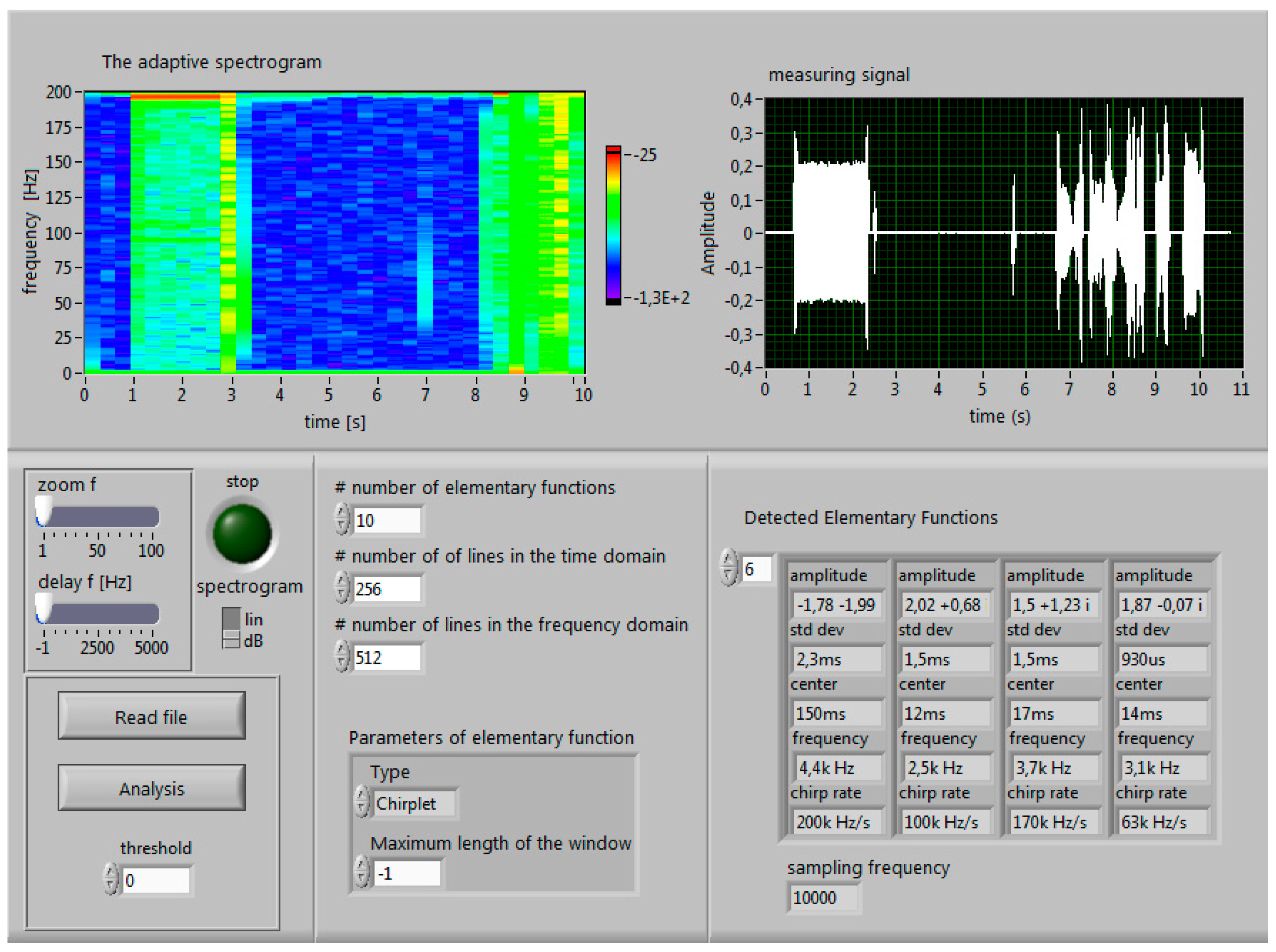
The MP method was applied in the virtual application, designed in LabVIEW software (version 2012, National Instruments Corporation, Austin, TX, USA) [22] (Figure 2). The numerical implementation of the presented method of the joint time-frequency analysis uses the LabVIEW library. There are VIs that implement an adaptive transform and adaptive expansion based on the MP algorithm. The discrete representation of the adaptive Gaussian function is defined by [22]:
The VI Adaptive transform.vi (Figure 3) is used to decompose an input signal into a linear combination of Gaussian chirplets, described by Equation (4). In Figure 3 the output Chirplet Info contains the parameters of each detected Gaussian chirplet elementary function, indicated in Table 1. This VI also outputs the normalized energy of the residue. The reconstruction of the examined signal, based on the designated matrix of chirplet parameters, is performed by Adaptive Expansion.vi. The total energy of the input signal and the normalized energy of the signal expansion are calculated as a variance of the values in the input signal and the signal expansion, respectively (Figure 3). The VI Standard Deviation and Variance.vi determines the output value using the following expression [22]:
where is the number of samples in a discrete input signal and is the average of the values in the input signal .
The numerical algorithm realizing an adaptive spectrogram of the signal is implemented in Adaptive spectrogram.vi. The adaptive spectrogram is computed by [22]:
3. The Optimal Size of the Dictionary in the MP Algorithm
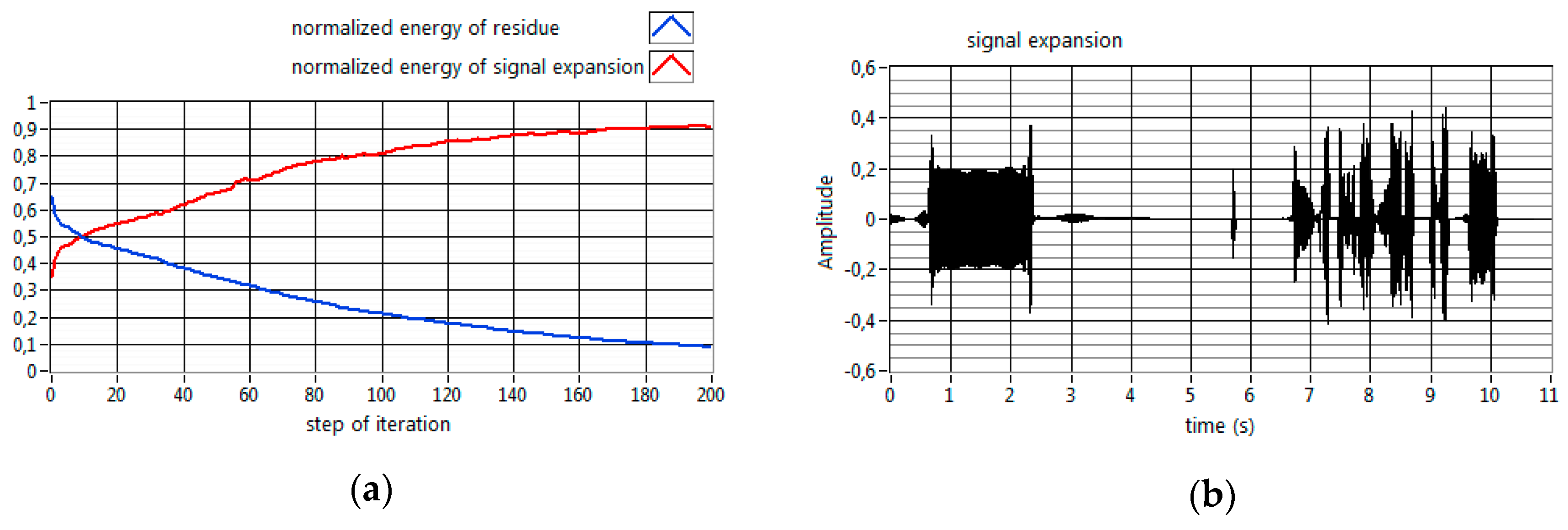
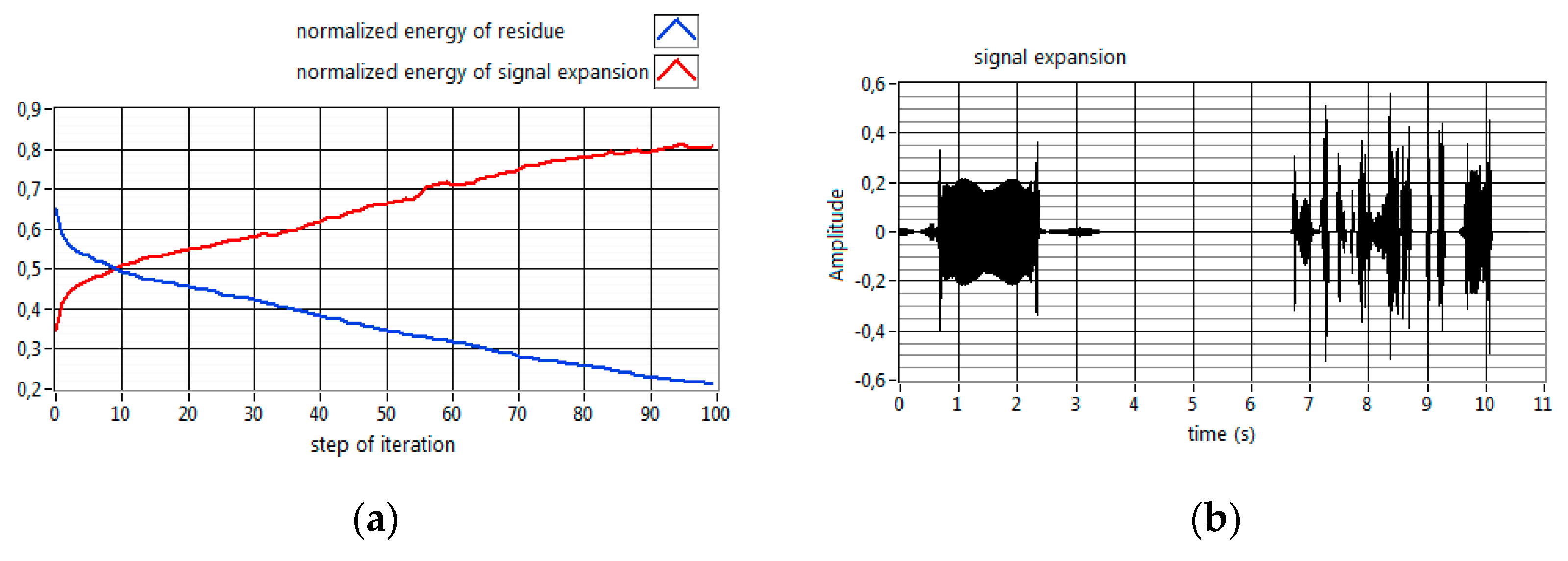
The value of residue in Equation (1) determines the approximation error of the expansion of the signal after choosing elementary functions from the time-frequency dictionary. It can be seen that the first few iterations of the algorithm separate the coherent parts of the signal, which are greatly correlated with atoms (Figure 4, Figure 5 and Figure 6). The remaining residue does not correlate precisely with any dictionary atoms and its features are affected by the attractor of the chaotic map [20]. For large numbers of atoms in the chirplet dictionary the residue meets a white noise realization and is fixed at an insignificantly low level (Figure 4). At each step of iteration, the variance (energy) of the residue and the variance of the signal expansion are estimated and its comparison can be used as a stopping criteria of the procedure. In case of the measured signal, which is considered in this paper, the reconstructed signal includes about 90% of the total energy of the original signal after 200 iteration steps but the continuing pursuit does not lead to error reduction (Figure 4).
The analysis of the parameters of each detected chirplet, such as the complex amplitude (Amplitude), the standard deviation of the Gaussian envelope (Standard Deviation), center time (Center), center frequency (Frequency) of the chirplet, and the chirp rate (ChirpRrate) (Table 1), are included in the matrix appearing at the output of Adaptive transform.vi (Figure 3) which allows for the indication of the dominant components in the adapted approximation of the observed signal. Figure 7 shows the part of the block diagram of the virtual analyzer that computes the normalized energy of the individual chirplets.
The subVI visualizes the time-waveform of each chirplet and calculates its spectrogram. The array containing the normalized energies of individual chirplets is obtained on the output of For loop of this subVI. Figure 8 presents the results of the analysis performed using the previously-mentioned subVI. The time-waveforms of single components of the signal expansion correspond to the selected chirplets. While running an MP algorithm, the elementary functions are chosen mostly in decreasing order of magnitude. The stopping criterion of the procedure is achieved when, in the next stage of the decomposition, a normalized energy of atom is smaller than an assumed threshold. In the case of the multicomponent signal, composed of distinct time-frequency structures, the MP procedure requires a large-sized dictionary and consistently becomes computationally inefficient.
The method that effectively allows the extraction of the dominant structure from the examined signal consists of the rejection from the aforementioned matrix of these chirplet atoms, whose energy is lower than a certain threshold.
Table 1 shows that the main chirplet in the reconstructed signal, which explains about 59% of total energy, is waveform no 1. Instead of calculating the adaptive spectrogram for a large number of atoms that belong to a redundant dictionary it is sufficient to process selected points of the chirplets. The choice of a threshold determines the computing speed and accuracy of the performing analysis. On the time-frequency planes of the spectrograms, estimated separately for each detected chirplet, the time-frequency structures coming out in the examined signal can distinctly identified (Figure 9).
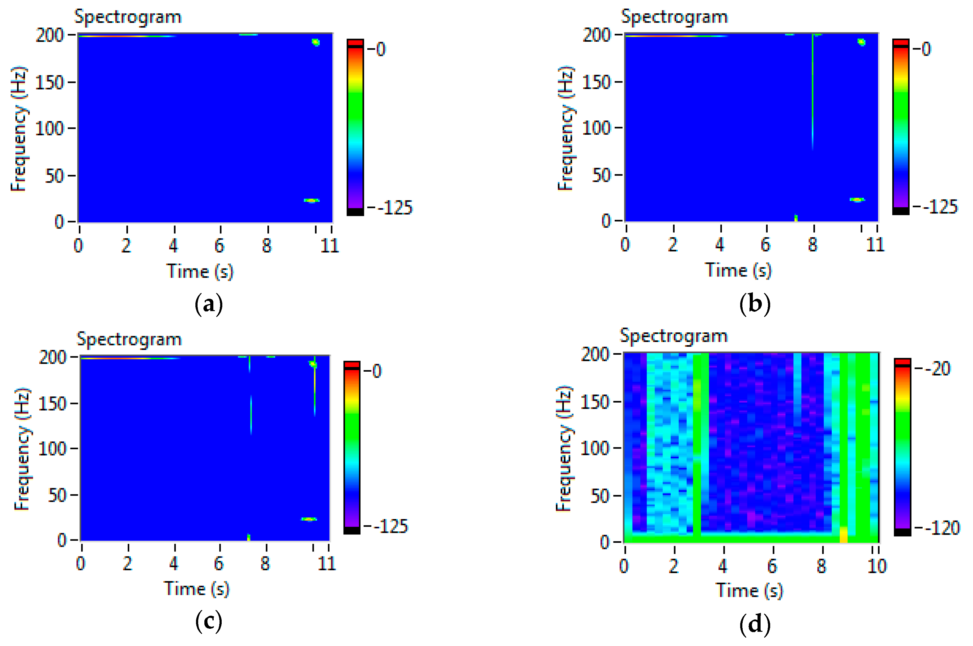
Figure 10 displays the spectrograms that are the results of an adaptive analysis for different sizes of dictionaries. The comparison with the previous figures (Figure 9) points out that effective identification of the dominant structures in the calculated spectrogram requires the additional preliminary processing of the signal expansion.
The dominant time-frequency signal structures, describing the features of observed signals, are indicated on the time-frequency plane of the resulting spectrogram.
4. The Method for Source Identification
Due to the previous considerations, the method of source identification can be stated as follows:
- Approximate a measured time-waveform into the linear expansion of chirplet atoms. The size of the dictionary chosen in the expansion of the measured signal is indicated on the basis of the percentage of the signal’s energy explained by the adaptive approximation. In practice, the approximation has good attributes if the reconstructed signal explains about 80% of the total energy. It emphasizes the coherence between the chirplet dictionary and most of the signal’s structures.
- Modify the obtained matrix containing the parameters of each detected Gaussian chirplet. Find the dominant components in the examined signal. Figure 11 shows the part of the block diagram of the virtual analyzer that examines the matrix of the chirplet parameter and computes the modified adaptive spectrogram. The normalized energy of single detected atom is compared with the inserting threshold. The rejection of a single chirplet is carried out using the procedure that compares the normalized energy of each elementary function with the threshold and removes the corresponding column of the matrix.
- Estimate the adaptive transform of the processed signal (the adaptive spectrogram). The calculation of the quadratic time-frequency representation of the signal is performed for the reduced matrix of the chirplet parameter.
5. Selected Analysis Results
The novel method of analysis has been applied for processing of real data, measured onboard of the vessel (Figure 12). The measurement procedure consists of two unattached steps.
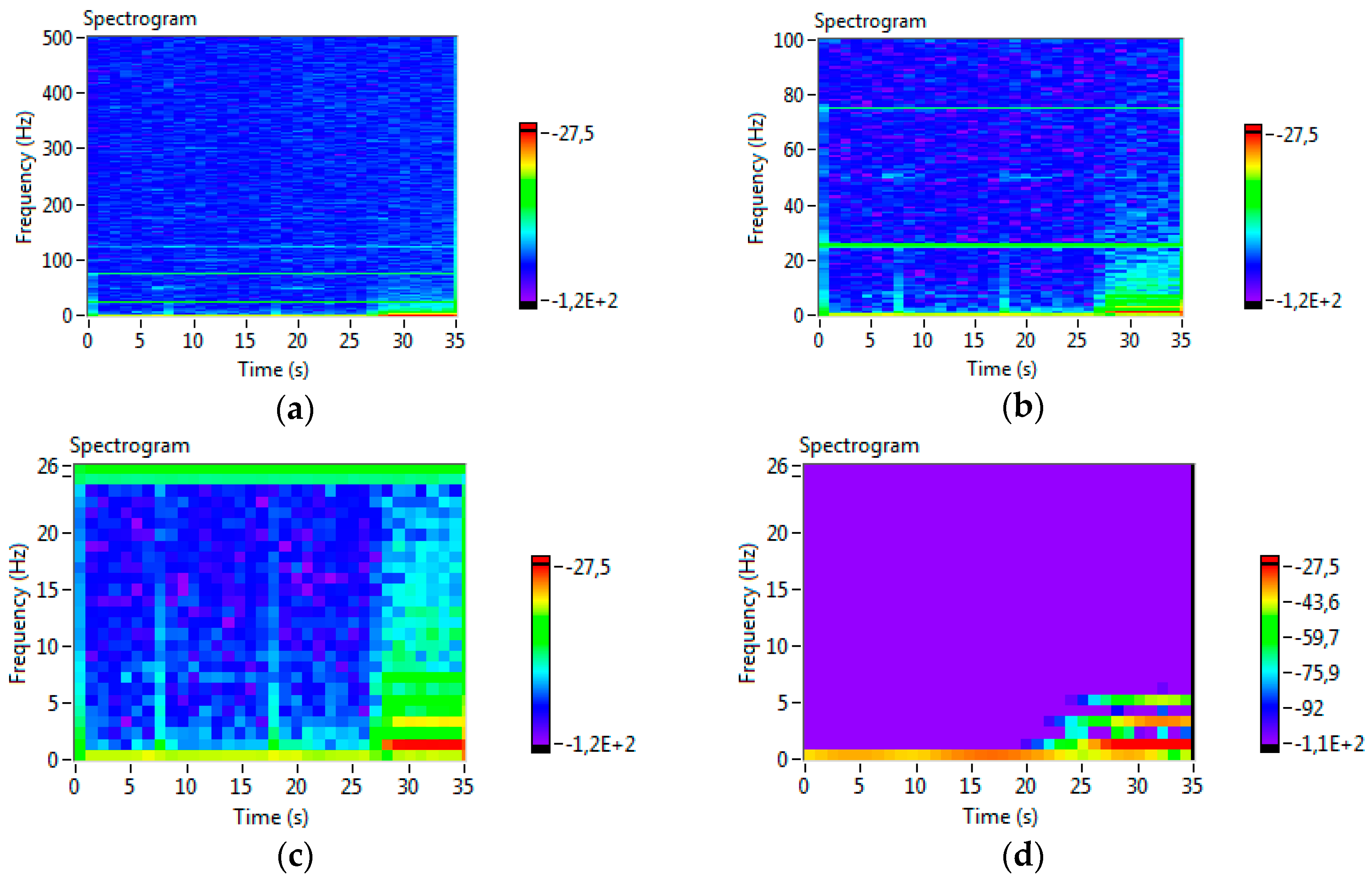
The acquisition of the time-waveforms corresponding to the instantaneous values of the MF induction was first performed. Then, the offline analyses, by means of a virtual application in the NI LabVIEW graphical environment, were carried out. The obtained results indicate that the highest level of the MF intensity occurs near the cable supplying the bow thruster motor. The recorded time-waveform for the short time-window in this measurement point is presented in Figure 13. The time-frequency representation corresponding to this signal shows that the dominant spectral components appear mainly in the low frequency range (Figure 14). The spectrograms are computed with 2048 lines of frequency and time, respectively. The size of the chirplet dictionary is equal to 100. Furthermore, stationary constituents, as well as nonstationary constituents of varied intensities, are visible in the time-frequency plane through the entire time. Note that the dominant time-frequency structures, appearing below 26 Hz, proves the existence of the main source of the MF density (Figure 14c). The obtained structures represent the signal component corresponded to the output frequency of the converter. The bow thruster is driven by the squirrel cage asynchronous motor, supplied from a frequency converter with an output frequency fixing within the frequency range from 0 to 30 Hz.
The modification of the chirplet matrix that consists in a rejection of more than 70 atoms in the signal approximation enables the calculation of the adaptive time-frequency transform for the smaller number of the elementary functions. The reconstructed signal still explains about 80% of the signal total energy. The resulting spectrogram for the size of the chirplet dictionary equals 25, and is illustrated in Figure 14d. In the time-frequency plane it is easy to find the signal structures corresponding to the frequency converter emitting the MF of the highest intensity.
The level of noise, occurring in the time-frequency representation of the measured signal has been significantly decreased at the same time. Moreover, the efficiency of the algorithm improved because of the computing speed.
6. Final Remarks
The new method of the MF source identification has been proposed in the paper. The chirplet MP algorithm has an advantage of decomposing a time-varying signal into a linear approximation of elementary functions that best adapt to signal structures. The size of a dictionary in the expansion of the analyzed signal is fixed on the basis of the percentage of the signal’s variance explained by the decomposition. The modification of the matrix, including the parameters of each chosen chirplet, enables the recognition of the main components in the signal expansion. The rejection of chirplets with the lowest normalized energy from the calculated matrix makes it possible to distinguish the dominant time-frequency structures on the plane of the resulting spectrogram. In this way, the sources of the magnetic field occurring in a measurement environment can be recognized. The proposed method is an efficient procedure for estimating an adaptive spectrogram with moderate processing time to identify the sources of the highest MF intensity.
Acknowledgments
The cost of publishing in open access is covered by the author’s employer (Gdynia Maritime University).
Conflicts of Interest
The author declares no conflicts of interest.
References
- Ahlbom, A.; Bergqvist, U.; Bernhardt, J.H.; Cesarini, J.P.; Court, L.A.; Grandolfo, M.; Hietanen, M.; McKinlay, A.F.; Repacholi, M.H.; Sliney, D.H. Guidelines for limiting exposure in time-varying electric, magnetic, and electromagnetic fields (up to 300 GHz). Health Phys. 1998, 74, 494–521. [Google Scholar]
- Karpowicz, J.; Gryz, K. Electromagnetic fields in the Polish legal system of managing ambient factors in the occupational environment. In Proceedings of the Workshop Measurements and Criteria for Standard Harmonization in the Field of EMF Exposure, Varna, Bulgaria, 28 April–3 May 2001. [Google Scholar]
- Palczynska, B. Spectral analysis of nonstationary low-frequency magnetic-field emissions from ship’s power frequency converters. In Proceedings of the Compatibility and Power Electronics CPE’09, Badajoz, Spain, 20–22 May 2009; pp. 375–380. [Google Scholar]
- Luo, X.; Shan, C.; Lv, G.; Yu, J. An efficient compensation method for ISAR imaging based on short time adaptive gaussian chirplet decomposition. In Proceedings of the IEEE Workshop on Advanced Research and Technology in Industry Applications (WARTIA), Ottawa, ON, Canada, 29–30 September 2014; pp. 891–894. [Google Scholar]
- Qing, Y.; Wang, J.; Sima, W.; Chen, L.; Yuan, T. Mixed Over-Voltage Decomposition Using Atomic Decompositions Based on a Damped Sinusoids Atom Dictionary. Energies 2011, 4, 1410–1427. [Google Scholar]
- Durka, P.J. Adaptive time-frequency parametrization of epileptic EEG spikes. Phys. Rev. E 2004, 69, 051914. [Google Scholar] [CrossRef] [PubMed]
- Ramya, S.; Hemalatha, M. A Review on Signal Decomposition Techniques. Middle-East J. Sci. Res. 2013, 15, 1108–1112. [Google Scholar]
- Puliafito, V.; Vergura, S.; Carpentieri, M. Fourier, Wavelet, and Hilbert-Huang Transforms for Studying Electrical Users in the Time and Frequency Domain. Energies 2017, 10, 188. [Google Scholar] [CrossRef]
- Khan, N.A.; Baig, F.; Nawaz, S.J.; Ur Rehman, N.; Sharma, S.K. Analysis of Power Quality Signals Using an Adaptive Time-Frequency Distribution. Energies 2016, 9, 933. [Google Scholar] [CrossRef]
- Khan, N.A.; Ali, S. Classification of EEG Signals Using Adaptive Time-Frequency Distributions. Metrol. Meas. Syst. 2016, 23, 251–260. [Google Scholar] [CrossRef]
- Chen, L.; Zheng, D.; Chen, S.; Han, B. Method Based on Sparse Signal Decomposition for Harmonic and Inter-harmonic Analysis of Power System. J. Electr. Eng. Technol. 2017, 12, 559–568. [Google Scholar] [CrossRef]
- Zhao, Y.; Li, Z.; Nie, Y. A Time-Frequency Analysis Method for Low Frequency Oscillation Signals Using Resonance-Based Sparse Signal Decomposition and a Frequency Slice Wavelet Transform. Energies 2016, 9, 151. [Google Scholar] [CrossRef]
- Mallat, S.G.; Zhang, Z. Matching pursuit with time frequency dictionaries. IEEE Trans. Signal Process. 1993, 41, 3397–3415. [Google Scholar] [CrossRef]
- Qian, S.; Chen, D.; Chen, K. Signal approximation via data-adaptive normalized Gaussian function and its applications for speech processing. In Proceedings of the ICASSP-92: 1992 IEEE International Conference on Acoustics, San Francisco, CA, USA, 23–26 May 1992; pp. 141–144. [Google Scholar]
- Gribonval, R. Fast matching pursuit with a multiscale dictionary of Gaussian chirps. IEEE Trans. Signal Process. 2001, 49, 994–1001. [Google Scholar] [CrossRef]
- Yin, Q.; Qian, S.; Feng, A. A fast refinement for adaptive Gaussian chirplet decomposition. IEEE Trans. Signal Process. 2002, 50, 1298–1306. [Google Scholar]
- Liu, Q.; Wang, Q.; Wu, L. Size of the dictionary in matching pursuit algorithm. IEEE Trans. Signal Process. 2004, 52, 3403–3408. [Google Scholar] [CrossRef]
- Palczynska, B. A Virtual Instrument for the Adaptive Analysis of Low-Frequency Magnetic-Field Emissions. In Proceedings of the IEEE 15th International Conference on Environment and Electrical Engineering, Rome, Italy, 10–13 June 2015; pp. 2159–2164. [Google Scholar]
- Palczynska, B. Application of matching pursuit based method to identify sources of time-vary magnetic field. In Proceedings of the IEEE 16th International Conference on Environment and Electrical Engineering, Florence, Italy, 7–10 June 2016; pp. 1–6. [Google Scholar]
- Bergeaud, F.; Mallat, S. Matching pursuit of images. In Proceedings of the International Conference on Image Processing, Washington, DC, USA, 23–26 October 1995; pp. 53–56. [Google Scholar]
- Ghofrani, S.; McLernon, D.C.; Ayatollahi, A. Comparing Gaussian and chirplet dictionaries for time-frequency analysis using matching pursuit decomposition. In Proceedings of the 3rd IEEE International Symposium on Signal Processing and Information Technology, Darmstadt, Germany, 14–17 December 2003; pp. 713–771. [Google Scholar]
- LabVIEW Advanced Signal Processing Toolkit Help, Adaptive Transform and Expansion. 2014. Available online: http://zone.ni.com/reference/en-XX/help/372656C-01/lvasptconcepts/tfa_adapt_trans_exp/ (accessed on 5 May 2017).
Figure 1.
The normalized energy of the residue as a function of number of iterations in MP algorithm for the adaptive expansion of the measured signal representing the MFD in surroundings of the ship’s motor drive during maneuvers. The size of the dictionary is equal to: (a) 30 and (b) 100.
Figure 1.
The normalized energy of the residue as a function of number of iterations in MP algorithm for the adaptive expansion of the measured signal representing the MFD in surroundings of the ship’s motor drive during maneuvers. The size of the dictionary is equal to: (a) 30 and (b) 100.
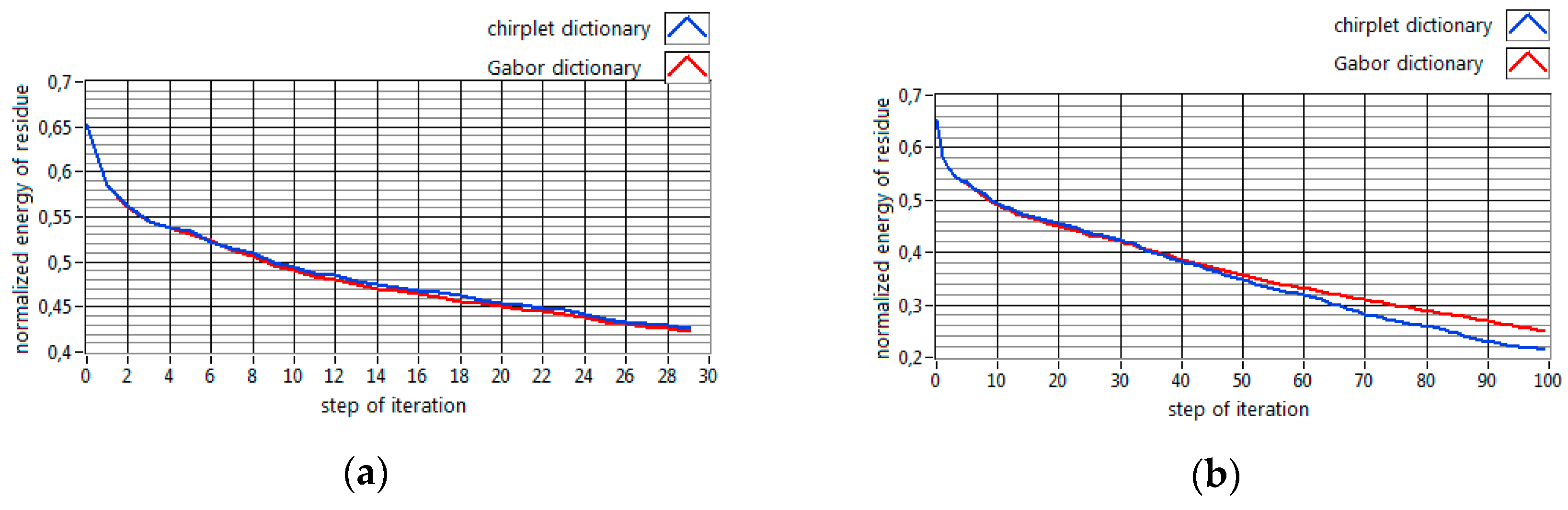
Figure 2.
The front panel of the virtual analyzer. It shows the time waveform of the measured signal, its adaptive spectrogram, and information about parameters of the detected chirplets. The measured signal represents the MFD in the surroundings of the ship’s motor drive during manoeuvers [18].
Figure 2.
The front panel of the virtual analyzer. It shows the time waveform of the measured signal, its adaptive spectrogram, and information about parameters of the detected chirplets. The measured signal represents the MFD in the surroundings of the ship’s motor drive during manoeuvers [18].

Figure 3.
The part of the block diagram of the virtual analyzer that calculates the components of the signal energy and outputs the matrix of the chirplet parameters.
Figure 3.
The part of the block diagram of the virtual analyzer that calculates the components of the signal energy and outputs the matrix of the chirplet parameters.
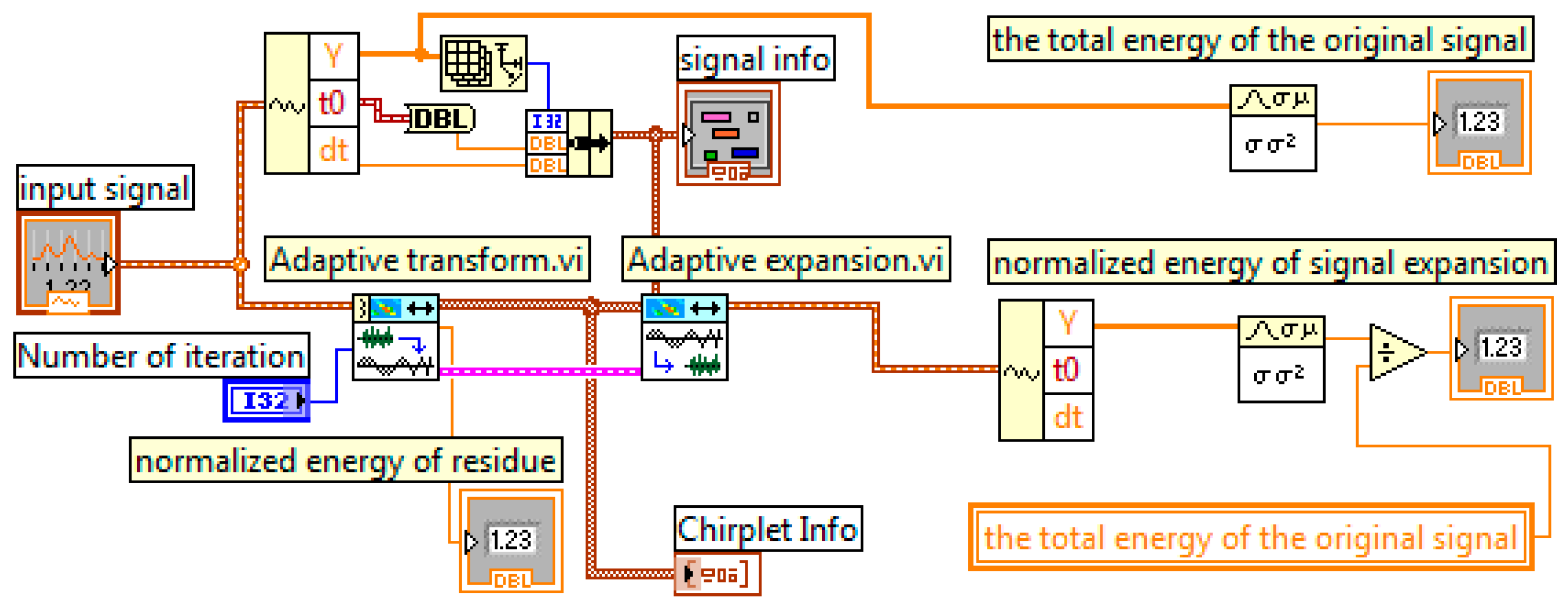
Figure 4.
The plots: (a) the normalized energy of the residue and the normalized energy of the signal expansion as a function of the iteration steps in the MP algorithm; (b) the reconstructed measured signal for dictionary size equal to 200.
Figure 4.
The plots: (a) the normalized energy of the residue and the normalized energy of the signal expansion as a function of the iteration steps in the MP algorithm; (b) the reconstructed measured signal for dictionary size equal to 200.

Figure 5.
The plots: (a) the normalized energy of the residue and the normalized energy of the signal expansion as a function of the iteration steps in the MP algorithm; (b) the reconstructed measured signal for dictionary size equal to 100.
Figure 5.
The plots: (a) the normalized energy of the residue and the normalized energy of the signal expansion as a function of the iteration steps in the MP algorithm; (b) the reconstructed measured signal for dictionary size equal to 100.

Figure 6.
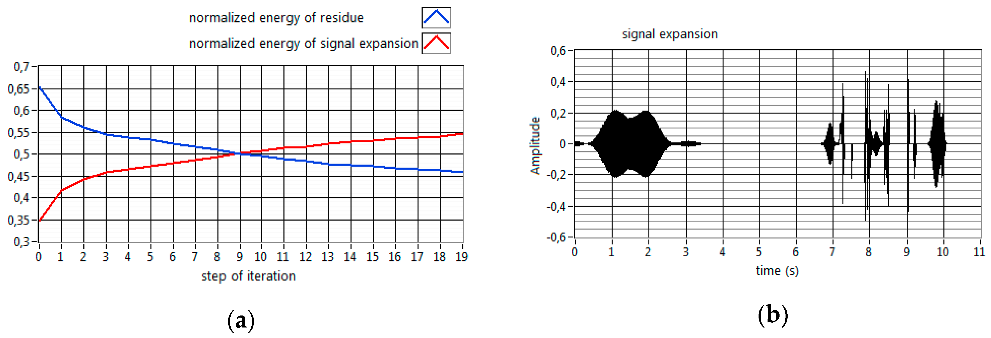
The plots: (a) the normalized energy of the residue and the normalized energy of the signal expansion as a function of the iteration steps in the MP algorithm; (b) the reconstructed measured signal for dictionary size equal to 20.
Figure 6.
The plots: (a) the normalized energy of the residue and the normalized energy of the signal expansion as a function of the iteration steps in the MP algorithm; (b) the reconstructed measured signal for dictionary size equal to 20.

Figure 7.
The part of the block diagram of the virtual analyzer, which calculates the normalized energy of each chirplet and computes its time-waveform and spectrogram.
Figure 7.
The part of the block diagram of the virtual analyzer, which calculates the normalized energy of each chirplet and computes its time-waveform and spectrogram.

Figure 8.
The time waveforms of the components of reconstructed signal representing chirlpet atoms described in Table 1: (a) chirplet no 1; (b) chirplet no 2; (c) chirplet no 3; (d) chirplet no 4; (e) chirplet no 5; (f) chirplet no 6; (g) chirplet no 7; and (h) chirplet no 8.
Figure 8.
The time waveforms of the components of reconstructed signal representing chirlpet atoms described in Table 1: (a) chirplet no 1; (b) chirplet no 2; (c) chirplet no 3; (d) chirplet no 4; (e) chirplet no 5; (f) chirplet no 6; (g) chirplet no 7; and (h) chirplet no 8.

Figure 9.
The adaptive spectrograms of the chirplet atoms: (a) chirplet no 1; (b) chirplet no 2; (c) chirplet no 3; (d) chirplet no 4; (e) chirplet no 5; (f) chirplet no 6; (g) chirplet no 7; and (h) chirplet no 8, presented on Figure 8.
Figure 9.
The adaptive spectrograms of the chirplet atoms: (a) chirplet no 1; (b) chirplet no 2; (c) chirplet no 3; (d) chirplet no 4; (e) chirplet no 5; (f) chirplet no 6; (g) chirplet no 7; and (h) chirplet no 8, presented on Figure 8.
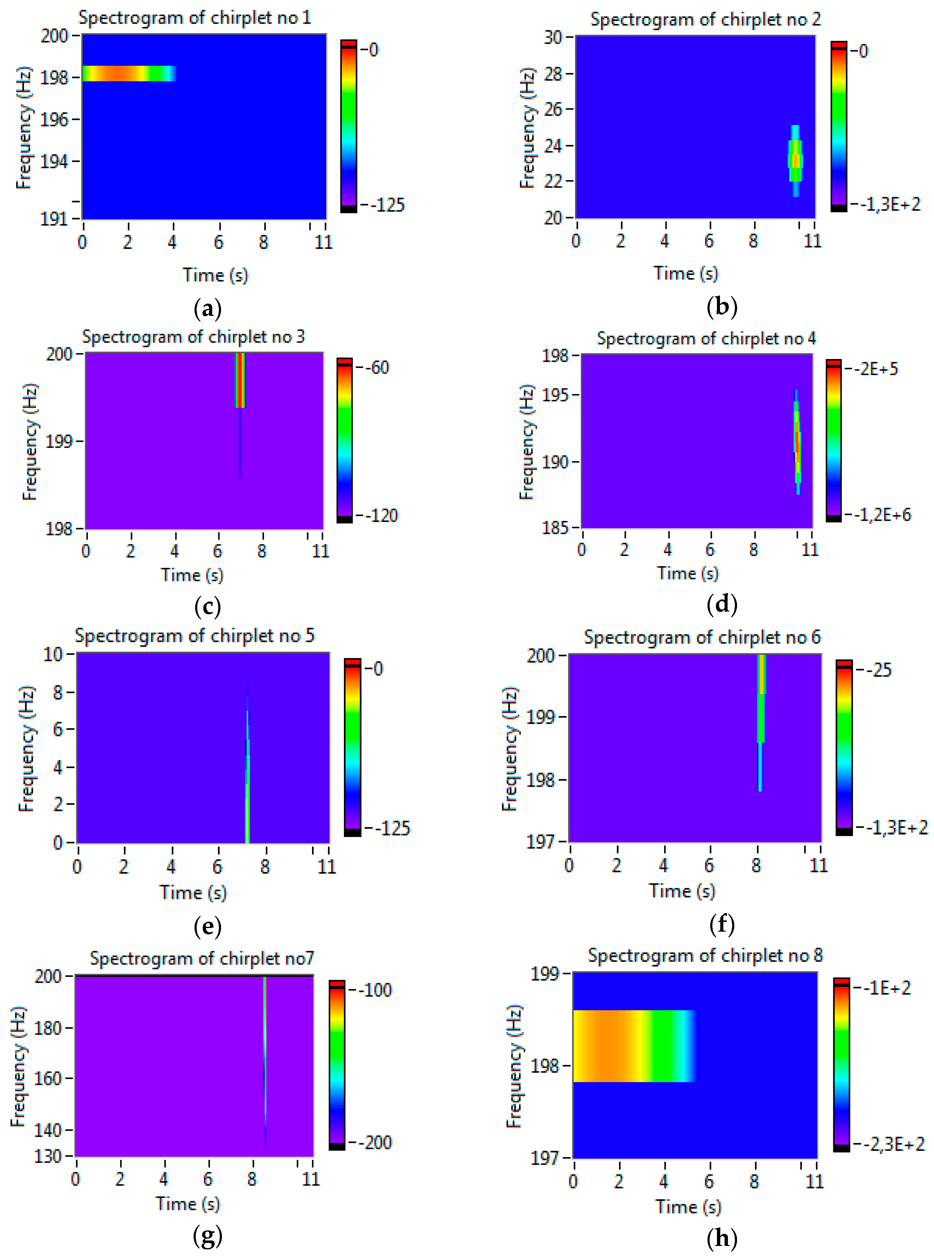
Figure 10.
The adaptive spectrograms of the adaptive expansions of the tested signal for the size of a dictionary equals to: (a) 4; (b) 20; (c) 50 and (d) 200, respectively.
Figure 10.
The adaptive spectrograms of the adaptive expansions of the tested signal for the size of a dictionary equals to: (a) 4; (b) 20; (c) 50 and (d) 200, respectively.

Figure 11.
The part of the block diagram of the virtual analyzer that modifies the matrix of the chirplet parameter and computes the modified adaptive spectrogram.
Figure 11.
The part of the block diagram of the virtual analyzer that modifies the matrix of the chirplet parameter and computes the modified adaptive spectrogram.
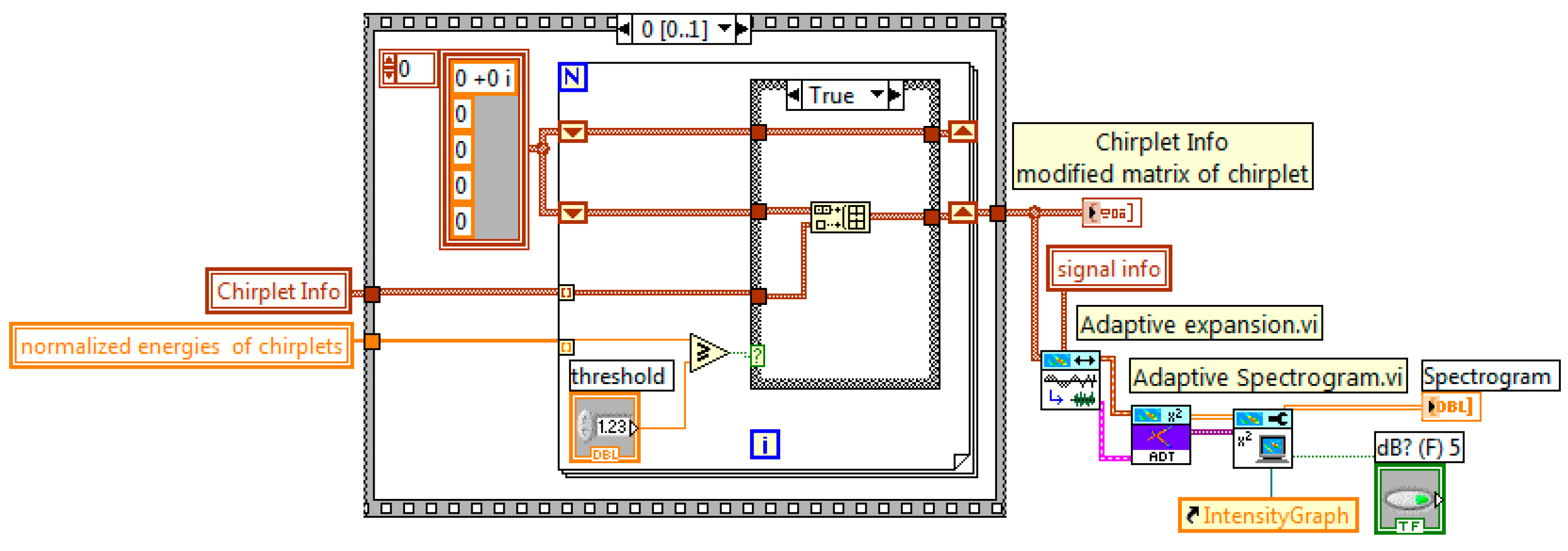
Figure 12.
The measurement points: (a) in the ship’s engine room, close to generators No 1 and No 3 and power transformers; and (b) in the ship’s fore part, close to the bow thruster motor [3].
Figure 12.
The measurement points: (a) in the ship’s engine room, close to generators No 1 and No 3 and power transformers; and (b) in the ship’s fore part, close to the bow thruster motor [3].
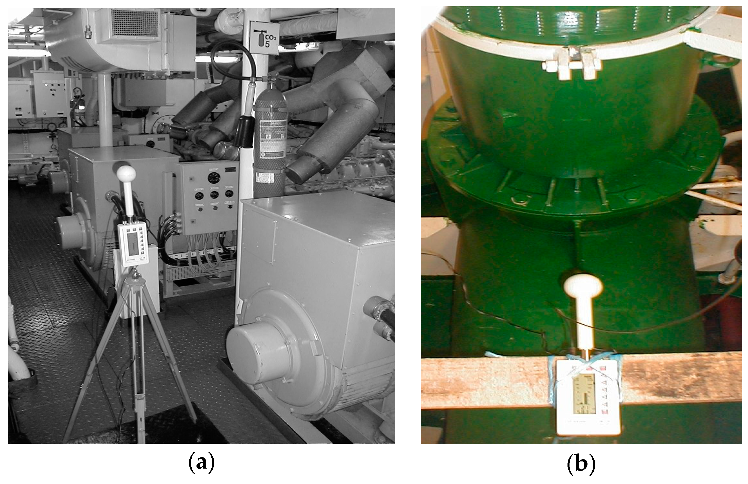
Figure 13.
The time waveform representing the MF induction recorded near the cable supplying the bow thruster motor. The sampling frequency is equal to 2000 Hz.
Figure 13.
The time waveform representing the MF induction recorded near the cable supplying the bow thruster motor. The sampling frequency is equal to 2000 Hz.
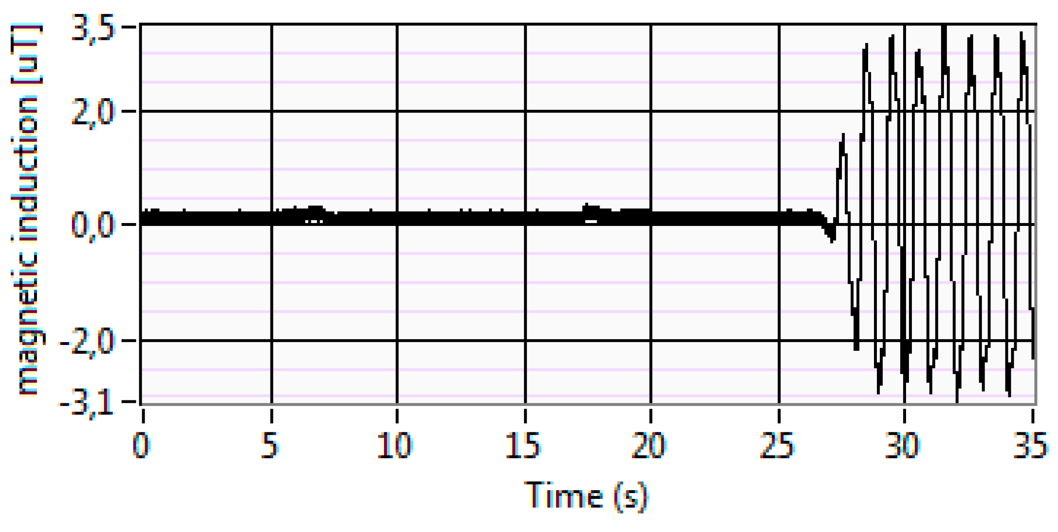
Figure 14.
The adaptive spectrogram of the signal in the frequency range: (a) up to 500 Hz; (b) up to 100 Hz; (c) up 26 Hz; and (d) up to 26 Hz after the rejection of the chirplets of low energy.
Figure 14.
The adaptive spectrogram of the signal in the frequency range: (a) up to 500 Hz; (b) up to 100 Hz; (c) up 26 Hz; and (d) up to 26 Hz after the rejection of the chirplets of low energy.


Table 1.
The parameters of detected chirplets for the first six atoms of the chirplet dictionary. The approximation was conducted for the measured signal representing the MFD in the surroundings of the ship’s motor drive during manoeuvers [18].
Table 1.
The parameters of detected chirplets for the first six atoms of the chirplet dictionary. The approximation was conducted for the measured signal representing the MFD in the surroundings of the ship’s motor drive during manoeuvers [18].
| Amplitude | Standard Deviation | Center | Frequency | Chirp Rate | Normalized Energy |
|---|---|---|---|---|---|
| 0.36 + 5.14i | 580 ms | 1.5 s | 198 Hz | 0 Hz/s | 0.59 |
| 2.16 − 0.78i | 76 ms | 9.8 s | 23 Hz | −1.6 Hz/s | 0.12 |
| −1.12 + 1.54i | 70 ms | 6.9 s | 199 Hz | −12 Hz/s | 0.044 |
| −1.1 + 0.22i | 37 ms | 10 s | 191 Hz | −47 Hz/s | 0.028 |
| 1.05 − 0i | 18 ms | 7.2 s | 4 Hz | 0 Hz/s | 0.012 |
| 0.93 − 0.3i | 79 ms | 8.2 s | 199 Hz | −52 Hz/s | 0.012 |
| −0.93 + 0.24i | 2.5 ms | 8.5 s | 170 Hz | −1 kHz/s | 0.013 |
| 0.56 + 0.73i | 900 ms | 1.5 s | 198.5 kHz | 0 Hz/s | 0.018 |
© 2017 by the author. Licensee MDPI, Basel, Switzerland. This article is an open access article distributed under the terms and conditions of the Creative Commons Attribution (CC BY) license (http://creativecommons.org/licenses/by/4.0/).
Share and Cite
MDPI and ACS Style
Palczynska, B. Identification of Non-Stationary Magnetic Field Sources Using the Matching Pursuit Method. Energies 2017, 10, 655. https://doi.org/10.3390/en10050655
AMA Style
Palczynska B. Identification of Non-Stationary Magnetic Field Sources Using the Matching Pursuit Method. Energies. 2017; 10(5):655. https://doi.org/10.3390/en10050655
Chicago/Turabian StylePalczynska, Beata. 2017. "Identification of Non-Stationary Magnetic Field Sources Using the Matching Pursuit Method" Energies 10, no. 5: 655. https://doi.org/10.3390/en10050655
Note that from the first issue of 2016, this journal uses article numbers instead of page numbers. See further details here.