
A Network Reconfiguration Method Considering Data Uncertainties in Smart Distribution Networks


Power Distribution Department, China Electric Power Research Institute, Beijing 100192, China
*
Author to whom correspondence should be addressed.
Energies 2017, 10(5), 618; https://doi.org/10.3390/en10050618
Submission received: 29 January 2017
/
Revised: 25 April 2017
/
Accepted: 26 April 2017
/
Published: 2 May 2017
(This article belongs to the Special Issue Electric Power Systems Research 2017)
Abstract
:This work presents a method for distribution network reconfiguration with the simultaneous consideration of distributed generation (DG) allocation. The uncertainties of load fluctuation before the network reconfiguration are also considered. Three optimal objectives, including minimal line loss cost, minimum Expected Energy Not Supplied, and minimum switch operation cost, are investigated. The multi-objective optimization problem is further transformed into a single-objective optimization problem by utilizing weighting factors. The proposed network reconfiguration method includes two periods. The first period is to create a feasible topology network by using binary particle swarm optimization (BPSO). Then the DG allocation problem is solved by utilizing sensitivity analysis and a Harmony Search algorithm (HSA). In the meanwhile, interval analysis is applied to deal with the uncertainties of load and devices parameters. Test cases are studied using the standard IEEE 33-bus and PG&E 69-bus systems. Different scenarios and comparisons are analyzed in the experiments. The results show the applicability of the proposed method. The performance analysis of the proposed method is also investigated. The computational results indicate that the proposed network reconfiguration algorithm is feasible.
1. Introduction
The distribution generation (DG) integration in distribution networks (DNs) has become a hot research topic. By allocating DG units at appropriate positions, load balancing and line loss minimization may be achieved after power flow optimization. In the meanwhile, DN structures may make necessary adjustments. After establishing a feasible radial distribution structure, DG units can be set with adjusted output in the reconfigured network to further improve the optimization results.
Network reconfiguration is the process of altering the open/closed status of sectionalizing and loop switches, thus adapting a new topological structure for reducing power losses and improving system reliabilities. The network reconfiguration process is often investigated under two circumstances: (1) reconfiguration for power service restoration; (2) scheduled reconfiguration due to seasonal variation and larger load changes. The former process is a nearly real-time optimization, while the latter can and should be planned before application. The essential motivation for reconfiguration is to reduce economic losses, which will take switch operation and mean time to restoration into consideration. From the perspective of distribution system operation, uncertainties are inevitable due to the sequential effects and environmental factors present in a DN. These uncertainties may be embodied as variability and incertitude in equipment and electrical parameters, such as fault rate of generators and load fluctuations.
As a non-differentiable constrained and non-linear programming problem, many algorithms have been proposed to solve the network reconfiguration issue. References [1,2,3,4,5] investigated how heuristic algorithms were applied in finding optimal network structures. Dai and Sheng [1] studied the network reconfiguration problem by combining a two-stage optimization problem, and only load data uncertainty was considered. Gomes and Carneiro [2] studied an improved heuristic algorithm to find optimal network structures. They took all weak loops into consideration at once and established a maneuvering list, then tried to open each weak loop according to the list, till the network became radial again. Gonzalez et al. [3] determined switch status by sensitivity analysis, thus avoiding repeated calculations. Zhang and Li [4] utilized the topology characteristic of networks to propose a heuristic method to determine the optimal solution after a short iteration. Rugthaicharoenchep et al. [5] applied a greedy algorithm to solve the multi-objective reconfiguration problem for power loss reduction and load balancing.
A considerable number of intelligent algorithms are also applied to reconfiguration problems. References [6,7,8] proposed three different methods derived from a genetic algorithm (GA) respectively. Prasad et al. [6] improved random evolution rules, making it possible to deal with discrete variables, and avoided islands and loops by improving encoding. Mendoza et al. [7] proposed accentuated crossover and directed mutation, reducing searching space and memory occupation. Enacheanu et al. [8] combined GA with graph theories to select an efficient mutation, making all the resulting individuals feasible.
As for other intelligent algorithms, Chang [9] proposed an application for the ant colony search algorithm in reconfiguration and capacitor placement. The algorithm kept the mutation towards optimization by setting pheromone-updating rules. Liu and Gu [10] proposed an improved discrete particle swarm optimization (PSO), in which they defined an efficiency index to evaluate feasible structures before applying the algorithm. Wu et al. [11] improved the integer coded PSO method by adding historically optimal solutions to new particle creation, directing the search to optimization.
To deal with uncertainties in DN systems, different methods had been investigated. Load uncertainty had been investigated in the recent literature. Lee et al. [12] proposed a two-stage robust optimization model for the distribution network reconfiguration problem with load uncertainty. Bai et al. [13] analyzed measured network data taking into account the issue of substation time-varying loads and uncertainty. Zhang and Li [4] utilized interval analysis in a heuristic method to demonstrate how uncertain parameters influenced the reconfiguration result. They chose reliabilities and economy as the main objectives instead of solely power loss optimization. Muñoz et al. [14] applied affine arithmetic method to a voltage stability assessment, and reduced the computation burden as compared to Monte Carlo simulations. Vaccaro et al. [15] presented a range arithmetic method for power flow problems including interval data. Rakpenthai et al. [16] utilized synchronized phasor measurement data and state variables expressed in rectangular forms to formulate the state estimation under the transmission line parameter uncertainties based on the weight least square criterion as a parametric interval linear system of equations.
DG units can be involved in the network operation as ancillary services [17,18]. To integrate DG in DN, the location and regulation for DG units are the main optimization problems in network reconfiguration [19,20,21,22]. Some representative methods were proposed in recent references. Pavani and Singh [23] allocated DG units on specific buses after the network had been optimized by a heuristic method, reducing the power loss on feeders. Rao et al. [24] applied a Harmony Search Algorithm (HSA) in DG setting combined with reconfiguration, and proved the method was effective under different load levels.
Although the attention of the previous works has been focused on those points mentioned separately, relatively little effort was directed to considering reconfiguration, reliability evaluation, interval analysis and DG allocation simultaneously. In this paper, the multi-objective network reconfiguration optimization model is formulated with the consideration of minimum line loss, minimum Expected Energy Not Supplied (EENS) and minimum switch operation cost, and then the optimization problem is solved by combining Binary Particle Swarm Optimization (BPSO) and HSA considering the DG placement. Further, interval analysis is applied to deal with equipment parameters and load data uncertainties.
The remainder of this paper is organized as follows: Section 2 formulates the proposed multi-objective optimization problem for network reconfiguration. The proposed method to solve the optimization problem is described in Section 3. Section 4 provides numerical results and comparisons of the proposed approach using multiple test systems with DG units. Section 5 summarizes the main contributions and conclusions of this paper.
2. Network Reconfiguration Problem towards Reliability and Power Loss Minimization
2.1. Objective Functions
2.1.1. Minimization of Line Loss Cost
The first objective is to minimize line loss cost in DN. The Forward and Backward Substitution Method (FBSM) is applied to compute the power flow in this paper. Iteration equations are given in forward process and backward process, respectively:
where and are the nodal current and voltage injection in the k-th iteration. and represent the branch current and voltage vector in the k-th iteration, respectively. and are admittance matrix and impedance matrix, is a function of the voltage vector standing for bus current injection caused by constant power load without perturbations [25,26], is the submatrix of adjacent matrix containing all the buses between substation and the bus being calculated.
The active power and reactive power between two neighbored nodes is as follows:
The line loss equation on feeders is described as follows:
where is bus voltage, and represent nodal real and reactive power outflow. and are the impedance of lower branch. and are real and reactive nodal power injection, respectively. and are the real and reactive power loss of node . is the total power loss in one hour. is the number of nodes.
Then the expression of power loss cost is as expressed:
where represents power loss cost in one year; is time periods in one year, and it normally equals to 24 × 365 (8760 h); and is electricity price. The electricity price d will vary with the market results.
2.1.2. Minimization of EENS
From the perspective of reliability enhancement, some utilities may aim at lowering System Average Interruption Duration Index (SAIDI), while others may prefer to reduce EENS. The EENS can be quantified as:
where is the average load connected at bus , and is defined as Annual Outage Time (AOT) [27]. AOT of bus can be calculated with equipment parameters as:
where is the total number of equipments at bus , and stand for annual equipment failure rate and average repair time, respectively. is k-th equipment on bus .
Equation (7) describes the method used to calculate AOT for a single bus. However in the radial network, upper buses will influence the lower ones. Since the network is radial, the load cannot be transferred to other feeders if the bus can’t be connected by other switches. Based on this prior knowledge, the AOT calculation should be modified as follows:
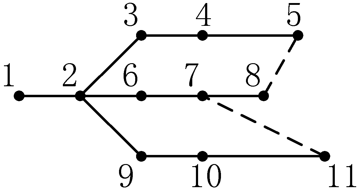
In order to demonstrate the problem clearly, a small system with 11 buses and three loops is taken as one example. As shown in Figure 1, the system contains 12 branches and 11 buses. Switches 5–8 and 7–11 are sectional switches. Three loops are formed when these switches are closed. The power supply point is numbered as 1, and the other buses are numbered orderly one by one. The branches are numbered the same as their end nodes. Sectional switches need to be numbered after all other branches.
- (1)
- Assuming that the trace begins at bus 5, calculate the failure rate on this branch. Then the failure rate of node 4 will influence node 5. Similarly, the failure rate of node 3 will influence node 4 and 5.
- (2)
- Determine related bus’ influence on the objective bus. For node 10, the node is connected only with node 9, and then the repair time of node 9 should be added to that of node 10. Otherwise it will be two conditions: For node 8, if its load can be transferred onto other feeder by connecting node 5 and node 8, then only a switch time should be added to node 10’s repair time. If the sectional switch can’t be operated at that time, we should still add node 7’s repair time to node 8.
2.1.3. Minimization of Switch Operation Cost
The switch operation cost contains many parts. The switch operation may bring damage to switch itself, thus reducing its life. At the same time, closing a switch will make the network run as a weak loop in a very short time, which may give rise to extra cost. All these costs can be quantified as operation cost q per time. Marking operation time as , the switch operation cost can be expressed as:
2.2. Constraints
2.2.1. Topology Constraint
2.2.2. Equality Constraint
The power flow equation should be satisfied after network reconfiguration, which can be described as follows:
where and are real and reactive load on bus . and are the real and reactive output of DG, which are treated as negative loads. is the nodal voltage on bus . and are the corresponding elements in nodal admittance matrix. is the power angle of bus .
2.2.3. Inequality Constraints
2.3. Treatment for Equality and Inequality Constraints
Power flow equations can be satisfied during the process of power flow computation. The inequality constraints for DG output can be satisfied in the encoding period. Through penalizing inequality constraints for bus voltage and current to the objective function, the constrained optimization problem can be transformed to unconstrained form of optimization problem, which can be expressed as follows:
Considering interval analysis, the objective function can be formed as:
where , and are weight factors for EENS, power loss and switch operation, while and are penalty factors for voltage and current constraints, respectively. The selections of weighting factor , and are from the preference of the decision maker. For the DN reconfiguration, the switch operation cost and EENS may be more concerned. By setting these weighting factors, the trade-off is established among the three objectives. and are the upper and lower bound of nodal voltage on bus . is upper bound of nodal current injection on bus .
3. The Proposed DN Reconfiguration Algorithm
3.1. Overview
Network reconfiguration with the consideration of DG placement is a combination of discrete and continuous problems. In this paper, a method is proposed to process the discrete and continuous variables, and then the problem is optimized comprehensively. To generate a feasible network topology, BPSO is applied to solve a multi-objective optimization of line loss and system reliability. Based on the given network, DG unit locations are chosen by sensitivity analysis. Further the sizing problem of DG units is optimized in HSA. HSA is a meta-heuristic algorithm inspired by the improvisation process of a musician. In HSA, each musician which represents a decision variable, plays a note, namely generates a value, to obtain a best harmony which represents the global optimum. HSA does not require initial values for the decision variables, and it has less parameters and is easy to implement. It has been successfully applied to various power system research problems.
3.2. Sensitivity Analysis with Loss Sensitivity Factors
Sensitivity analysis is often utilized in DG placement [28]. The candidate locations for DG units are determined by calculating the sensitivity factors of buses in the network. This process will help narrow the search space for the optimization procedure.
The sensitivity factor can be defined as the derivation form of Equation (3). Since the factor is the derivative of power loss with respect to bus load, the factor is called Loss Sensitivity Factor (LSF), which can be expressed as:
Based on Equation (14), the LSFs of all buses can be calculated and arranged in descending order. The order determines the priority of buses to be considered as DG locations. After the candidate buses are chosen, the size of the DG can then be calculated using HSA.
3.3. DG Modeling
This paper is concerned with DG output planning and not real-time dispatching, which means a DG model which can be smoothly adjusted while keeping power factor stable is required. Based on this consideration, a wind turbine (WT) is chosen as a typical model.
Different types of WTs are applied under different circumstances including synchronous generator (SG) and asynchronous generator (AG). Among them, the Doubly Fed Induction Generator (DFIG) is chosen as the DG model in this paper. These generators can smoothly adjust their real power output, while keeping power factor stable with reactive power compensation equipment. Then the DG units can be modeled as negative PQ-type loads:
where and are the real and reactive power load at node after the DG is placed. and are the real and reactive power output of DG units, respectively.
3.4. Generating Feasible Solution Algorithm Using BPSO
BPSO is a binary version of the PSO algorithm in which a velocity limitation would be needed to make sure solutions don’t fall into local optima. In this paper, BPSO is utilized to search for feasible network reconfiguration solutions. The sigmoid function is utilized to reflect the mapping relation between particle velocity and probability to be chosen, and ensures the result to be global optimal. The procedure of BPSO can be described as follows:
- Step (1)
- Describe the status of all switches as array containing only 0 and 1, which means open and closed status respectively. Calculate objective function value for the initial system with , save the evaluation index.
- Step (2)
- Generate the adjacent branch matrix and bus incidence matrix of the system. Search for loops formed by closing sectional switches, and save the loops as arrays .
- Step (3)
- Generate the particle swarm: for every loop in , after all the loops are opened, a new particle is then formed. In BPSO, the location and velocity of particles are expressed as two vectors. Location represents the switch status and velocity influences the possibility for location to change, which can be expressed as:where is the dimension of particles.
To deal with opening loop process, the displacement formula of BPSO is as follows:
where is threshold, typically set to 0.5 as default. The open switch is randomly selected among the zero elements of array in each loop. After the selection, a new particle is formed. The loops in may have overlay parts, so rules must be made to avoid them from choosing the same switch to open.
After a particle is formed, it needs to be checked by topology analysis to make sure that it represents a feasible solution.
- Step (4)
- Repeat Step 3 until the swarm size meets the requirement.
- Step (5)
- Generate solutions using BPSO and perform a topology analysis. Calculate the objective function value and save the evaluation index including power loss, reliabilities, total cost, etc. If the evaluation index of the solution is better than the historically best one, the index will be updated.
- Step (6)
- Do Step 5 until the iteration reaches the maximal iteration , or the required accuracy is satisfied. Output the best index and the topology structure.
3.5. Topology Analysis
Topology analysis can detect whether the network generated by BPSO has loops or islands. Since the particle generating process determines that the network must be open loop, the system will not contain any closed loops. The topology analysis is applied to detect islands in the system.
As a network generated by BPSO, its bus incidence matrix is marked as B. Each row shows the connection between one certain bus and all others, in which 1 means connected and 0 unconnected. The sum of each row is the grade of each node, which denotes the connection relation extent between this node and others. Apparently, the grade of an isolated bus is 0. The head or end node of the network is 1. The grade of other nodes is equal or greater than 2. The demonstration of topology analysis is based on the 11-bus system shown in Figure 1. The node incidence matrix when the system is running in normal status is shown as:
The proposed method to find island system is as follows:
- Step (1)
- Calculate grades of all the nodes in node incidence matrix B. Check if there is any node with grade 0. If the grade of any node is equal to 0, then it denotes that there is island node, which means the formed network structure is not feasible;
- Step (2)
- If there is no island node, then delete the maximal node number with grade that equals to 1, namely deleting the corresponding row and column, and go to Step 1;
- Step (3)
- Repeat step 1~2 until the network has only two nodes. If they aren’t nodes whose grade equals to 0, the network structure is proved to be feasible.
The process will reduce the rank of matrix B by 1 each time. For example, after utilizing the above method for 4 times, the matrix is shown as:
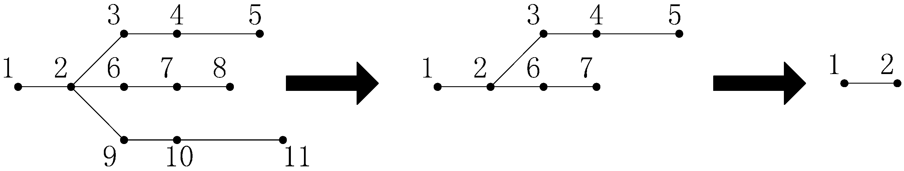
In the residual matrix, rows (or columns) representing grade-1 buses are 1, 5 and 7, namely the buses 1, 5 and 7 in the original system. Step 2 only reduces the system’s dimension, while keeping its topology structure. As the procedure continues, the matrix will finally become a 2-bus system, and the grades of remaining buses are both 1, which meets the termination condition of the operation. This proves that the original network structure doesn’t contain any islands. The process in topology structure is shown in Figure 2.
3.6. Interval Analysis Method
To deal with uncertain factors in different mathematic models, interval analysis was proposed by Moore [29]. The basic principles in interval calculation are as follows:
where and represent two sets. In Moore’s theory, the interval calculation can be done by using only their bounds, namely . Based on this, the elementary operations are theoretically described in Equation (20). These operations represent add, subtract, multiply and divide in interval calculation respectively. In power systems interval analysis is usually applied in power flow calculations. The method varies in different algorithms. In recent research, some researchers proposed different methods to deal with interval data in power system. In this paper, interval analysis is applied into FBSM. There are two procedures in each iteration, which can be described as follows:
- (1)
- Backward process: From the interval voltage vector of bus and interval current vector into bus k, calculate the interval voltage vector of bus and interval current vector out of bus .
- (2)
- Forward process: From the interval voltage vector of bus and interval current vector out of bus , calculate the interval voltage vector of bus k and interval current vector into bus .
By applying the interval calculation principles in the Equations (1) and (2) mentioned in Section 2, the interval form of FBSM is given as:
From the equations shown above, each variable appears only once in every FBSM iteration, thus keeping the interval calculation not so conservative. As for complexity, the interval FBSM costs only two times more than that the traditional FBSM, while the Newton method needs more memory space and calculation time to update the modified matrix. If the optimal solution is in interval form, then an intervals comparison is inevitable. For two intervals [A] and [B], it’s easy when [A] and [B] don’t share any common part. If they do have an overlapped area, then we pick two random variables from [A] and [B], respectively. Mark as event P, and assume values in the two intervals are uniformly distributed. The probability of P then can be calculated to evaluate the coverage of [A] on [B]. After this process, the result can be compared and optimization can be achieved.
3.7. Optimal DG Sizing Based on HSA
HSA can deal with continuous variables with the merit of many stochastic optimization methods [30]. To optimize sizing after network reconfiguration, the process of applying HSA is as follows:
- Step (1)
- Save the optimal network structure output by BPSO as array , and generate the HSA objective function with . Multiple DG capacities are set as independent variables.
- Step (2)
- Generate initial harmony vectors. The parameters need to be given before initialization process are: Harmony Matrix (HM); Harmony Memory Size (HMS), Harmony Memory Considering Rate (HMCR), Pitch Adjusting Rate (PAR), and Number of Improvisations (NI).
- Step (3)
- Improvise a new harmony vector.
In this step, PAR is defined as a dynamic value, and a coefficient factor is also defined as follows:
where , and are the ranges of PAR; is the current iteration number; is the maximum number of iterations; and are the bounds of . is defined as:
With the improvement in (22) and (23), PAR and fw can adapt themselves to the optimization as the HSA iteration goes on: in the early iterations, new values within a wide range can be easily added into HM; in the later iterations, as the vectors become closer to an optimal solution, the parameters will reduce their step size, thus making the adjustment more precise.
- Step (4)
- Update harmony memory.
- Step (5)
- Check if the iteration reaches the maximum iteration tmax 2. If the current iteration number is less than tmax 2, then go to Step (3); otherwise output the result.
3.8. The Flow Chart of the Proposed Solution
The flow chart of the proposed Algorithm 1 is shown in the following pseudo codes:
| Algorithm 1. Procedures of the proposed BPSO & HSA |
| Input: Initial switch status, BPSO population size Npop, maximal iteration tmax 1 and tmax 2, etc. |
| Output: Optimal solution (optimal switch status, DG locations and sizing) |
| 1: Initialize BPSO variable vector, and set iteration number t = 0; |
| 2: Power flow and reliability computation, save performance index; |
| 3: Generate particle swarm. |
| 4: while t < tmax 1 do |
| 5: Generate particle swarms. Start searching solution; |
| 6: Do topology analysis, if not feasible, go to 5; |
| 7: Power flow and reliability computation, compare the index with historical ones, update index; |
| 8: t = t + 1; |
| 9: end while |
| 10: Save the best solution as NodeInfo representing optimal network structure, reset t to 0; |
| 11: Make sensitivity analysis, and determine DG locations; |
| 12: Initialize HSA variable vector and memory, generate target function with NodeInfo; |
| 13: while t < tmax 2 do |
| 14: Improvise new harmony vector; |
| 15: Update harmony memory; |
| 16: t = t + 1; |
| 17: end while |
| 18: Save the best vector representing optimal DG sizes. |
| 19: return optimal solution. |
| 20: end |
4. Experiments and Analysis
4.1. Experiment Setting
To demonstrate the effectiveness of the proposed algorithm, the IEEE 33-bus and PG&E 69-bus are tested utilizing it. The algorithm was implemented, evaluated and compared in the following environments:
- (1)
- Four scenarios are set to be investigated in network reconfiguration as follows: (I) the system is in normal status; (II) only reconfiguration is considered, and interval analysis is utilized by using interval data; (III) DG units are integrated in the system without the consideration of reconfiguration, with only crisp result; (IV) Both DG integration and reconfiguration are all considered in the system.
- (2)
- In the experimental settings, the electricity price is set to 0.3 $/kWh, and switching cost of each switcher is set to 3.7 $. The weight factors for EENS, power loss and operation cost , and are set to 25, 1 and 5000 respectively. Penalty factors and are both set to 1.0 × 10⁵. In the experiments, minimum nodal voltage (in p.u.) is also listed as additional evaluation index.
- (3)
- In BPSO, the particle swarm population is set to 600, and maximal iteration number is set to 30. In HSA, parameters are set as HMS = 6, HMCR = 0.9, PAR [0.4, 0.9], NI = 3000. All the scenarios are simulated in MATLAB.
- (4)
- The algorithm verification and comparison were made with Neighborhood Search Algorithm (NSA) [4], Heuristic Algorithm (HA) [23], classical HSA [24] and commercial software CYMEDIST. In HA, the voltage upper constraint was set to 1.05. In classical HSA, the parameters are set as HMS = 20, HMCR = 0.85, PAR = 0.3, NI = 180, respectively.
4.2. Test Case on IEEE 33-Bus
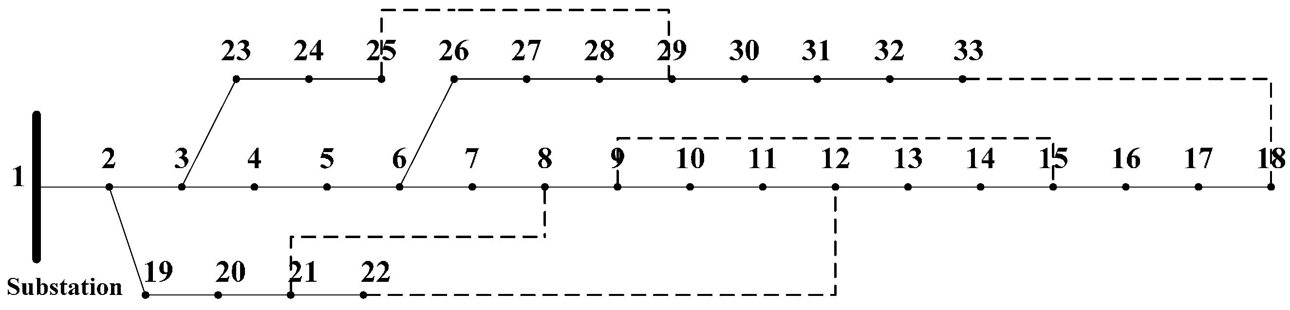
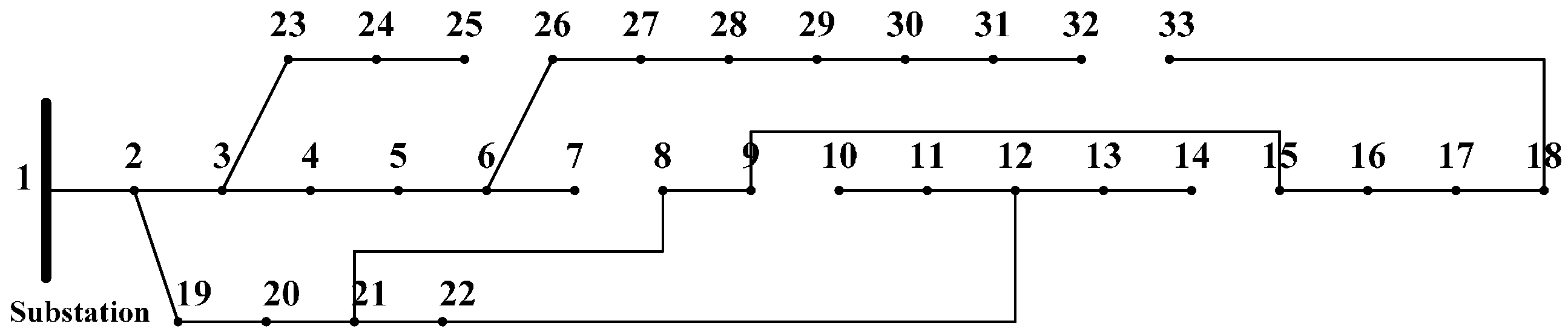
As shown in Figure 3, the IEEE 33-bus system is a standard 12.66 kV radial DN with 33 tie switches and five sectional switches [31]. Its total active power and reactive power are 3.715 MW and 2.3 MW, respectively. Integration of DG units with power ranging from 0 to 2 MW is considered. The reliability parameters are shown in Table 1, and 10% variation is included to simulate the interval analysis. The bus data of IEEE 33-bus refers to [31]. Solutions of different scenarios are shown in Table 1. The topology of the optimal solution in Scenario IV is shown in Figure 4, and the voltage profile is shown in Figure 5.
As shown in Table 2, the improvement in Scenario IV proves to be more significant than in Scenarios II and III. In Scenario IV, the power loss is 63.80 kW, compared with 129.83 in Scenario II and 68.54 in Scenario III. The percentages in Table 2 refer to the reduction compared with the corresponding value in Scenario I. The EENS is reduced from 2709.4 to 2694.5, and it’s mainly influenced by network structure, which explains why it stays the same in Scenarios II and IV. Nevertheless, the minimum voltage of the system is also improved in Scenario IV.
With the proposed method, it can be seen that DG installation after reconfiguration is proved to be more effective than simply applying one of them into system. As shown in Figure 5, DG installation significantly improves the voltage profile in Scenario III, and even better in Scenario IV when combined with reconfiguration. This is because reconfiguration can only change the status of certain switches to perform a limited optimization, while DG units can smoothly adjust the load distribution by changing the real and reactive output and achieve an even better result.
4.3. Comparison Analysis of the BPSO&HSA Algorithm
A comparison between the proposed method and other algorithms is made for different scenarios. In Scenario II, NSA [4], HA [23], classical HSA [24] and CYMEDIST are compared in crisp results, while NSA is also compared in interval results. In Scenario IV, classical HSA and HA are compared. The network parameters and reference voltage are the same in those algorithms, and the algorithm parameters are set to their default values.
As shown in Table 3, the proposed method has a power loss reduction of 32.02%, compared with other methods. BPSO&HSA’s interval result is also better than NSA. The improvement possibility (IP) in Table 3 means the definition of interval comparison mentioned in Section 3, which represents the probability that the result after optimization will be improved.
For Scenario IV, it shows that the proposed method has reduced power loss by 66.60%, better than HSA. HA gets a better power loss reduction result than the proposed method, but it is worth noticing that the HA simulation runs under milder conditions, in which they set a higher upper bound for bus voltage. As a higher bus voltage can be tolerated, power loss reduction will be easier to improve.
4.4. Test Case on PG&E 69-Bus
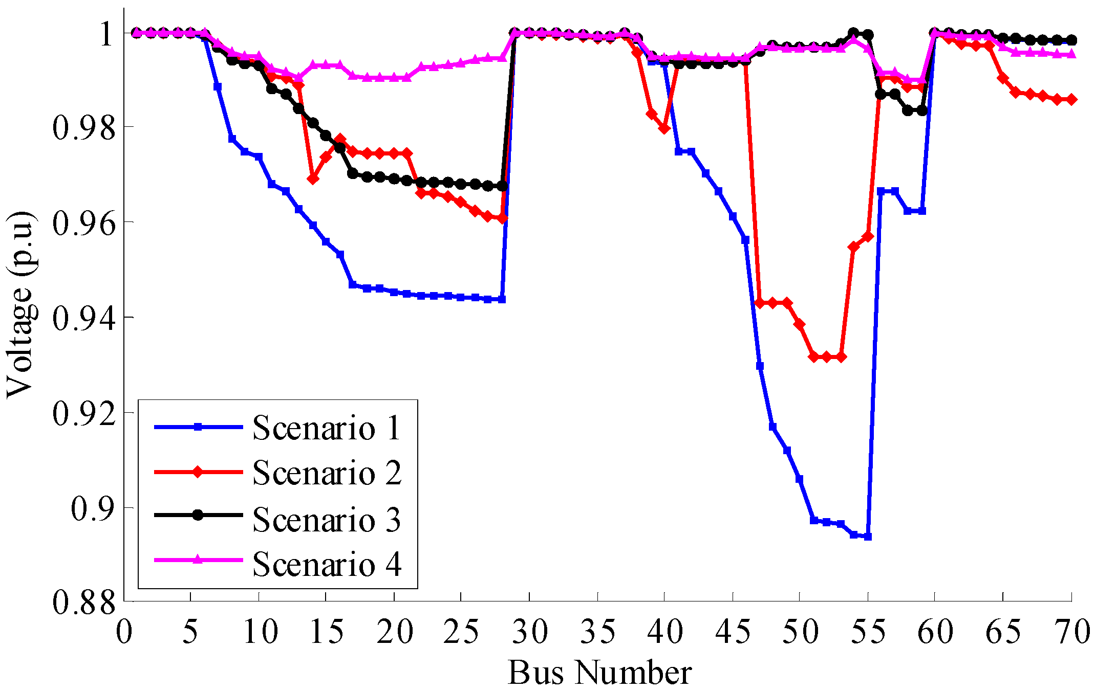
The proposed method is also tested on the PG&E 69-bus system, which is a standard 12.66 kV DN, with 69 tie switches and five sectional switches [32]. Its total active power and reactive power are 3.802 MW and 2.694 MW, respectively. Three DG units with active power ranging from 0 to 2 MW are considered for integration in the system with the network reconfiguration. The parameter settings are the same as Section 4.2. Since there is no available reference about interval data for the PG&E 69-bus test system, the interval original data is derived from crisp data with a volatility of 15% in this paper. The topology of the optimal solution in Scenario IV is shown in Figure 6, and the voltage profile is shown in Figure 7.
The solutions for different scenarios are shown in Table 4. The percentages in Table 4 refer to the reduction compared with the corresponding value in Scenario I. The power loss reduction in Scenario IV proves to be more significant than in Scenarios II and III. Since any reliability improvement is concerned with the network structure, the EENS reduction in Scenarios II and IV are both 991.4, which is more effective than in the IEEE 33-bus system. This is because reconfiguration will adjust load distribution more effectively in the PG&E 69-bus system. In addition, DG installation sharply reduces the power loss up to 95.23%, namely only 5.77% of the base case, when combined with reconfiguration in Scenario IV.
4.5. Further Analysis of BPSO&HSA Algorithm on PG&E 69-Bus System
Since BPSO and HSA are both intelligent stochastic algorithms, the parameter values need to be tuned to optimize the computational performance. Experiments are made with different parameters to make a performance comparison. In BPSO, the most influencing parameters are swarm dimension and iteration number. Scenario II is chosen as the simulation scenario so that BPSO can be tested without the effect of HSA. In the PG&E 69-bus system, the results of different parameters in Scenario II are shown in Table 5.
As shown in Table 5, reducing the swarm dimension and iteration time will shorten the computation time at the cost of obtaining non-optimal results. With the proposed parameter settings, BPSO will reach the optimal solution in about 25~30 iterations. In order to get the optimal result, the iteration number should therefore be set to 30. It also shows that higher iteration number settings won’t bring any advantages but just cost more computation time.
In HSA, the crucial parameters are HMS and NI. Scenario III is chosen so that HSA can be tested without the effect of BPSO. Since HSA is utilized to solve a continuous variable problem, the result in Table 6 is an average value of five runs with different random seeds. In the PG&E 69-bus system, the results of different parameters in Scenario III are shown in Table 6.
Like other stochastic algorithms, HSA can converge to get an optimal solution with a relatively long computation time. As shown in Table 6, the comparison result shows that HMS is a more sensitive parameter than NI. Increasing the NI number will not bring any further substantial improvement in the computation result. On the other hand, a smaller memory size or iteration number will obtain non-optimal solutions.
5. Conclusions
The distribution network reconfiguration problem with data uncertainty is investigated in this paper. With the consideration of DG allocation and switch status reconfiguration, the three objectives have been formulated as minimal line loss cost, minimal reliability index and minimal switch operation cost. A two-stage optimization method for distribution network reconfiguration has been proposed with the uncertainties of load and device parameters. The first-stage process is to utilize BPSO to get candidate solutions by using topology analysis. In the first-stage process, the interval analysis is used in the FBSM power flow. The second-stage decision is to find the optimal DG allocation with the reconfigured network by utilizing HSA. The main contributions of this paper can be further summarized as follows:
- (1)
- A multi-objective reconfiguration planning algorithm is proposed in this paper. The multi-objective considerations include power loss, EENS, switching operations, DG placement, etc.
- (2)
- Interval analysis is utilized in BPSO, making it possible to deal with uncertainties in reconfiguration problems, including equipment reliability, load uncertainty, etc.
- (3)
- An effective topology analysis method is proposed for open-loop systems. Different from the traditional methods, the proposed method makes use of the open-loop rules, thus skipping loop-detection part and focusing on detecting islands. The proposed topology analysis can be referred in the large scale network analysis.
Acknowledgments
This work was supported in part by the National Natural Science Foundation of China (Grant No. 51377148) and State Grid Corporation of China Research Program (Grant No. PD-71-15-042), and their financial support is much appreciated.
Author Contributions
Ke-yan Liu put forward the main idea and designed the entire structure of this paper. Yongmei Liu and Ke-yan Liu did the experiments and prepared the manuscript. Wanxing Sheng and Xiaoli Meng guided the experiments and paper writing.
Conflicts of Interest
The authors declare no conflict of interests.
References
- Dai, W.; Sheng, W.X.; Liu, K.Y.; Sheng, Y.; Ye, Z.J. A novel reconfiguration method in smart distribution grid considering interval data and distributed generation. In Proceedings of the International Conference on Computer Information Systems and Industrial Applications (CISIA 2015), Bangkok, Thailand, 28–29 June 2015; pp. 25–28. [Google Scholar]
- Gomes, F.V.; Carneiro, S.; Pereira, J.L.R.; Vinagre, M.P.; Garcia, P.A.N.; Araujo, L.R. A new heuristic reconfiguration algorithm for large distribution systems. IEEE Trans. Power Syst. 2005, 20, 1373–1378. [Google Scholar] [CrossRef]
- Gonzalez, A.; Echavarren, F.M.; Rouco, L.; Gomez, T. A sensitivities computation method for reconfiguration of radial networks. IEEE Trans. Power Syst. 2012, 27, 1294–1301. [Google Scholar] [CrossRef]
- Zhang, P.; Li, W.Y.; Wang, S.X. Reliability-oriented distribution network reconfiguration considering uncertainties of data by interval analysis. Int. J. Electr. Power Energy Syst. 2012, 34, 138–144. [Google Scholar] [CrossRef]
- Lantharthong, T.; Rugthaicharoenchep, N. Network reconfiguration for load balancing in distribution system with distributed generation and capacitor placement. J. Energy Power Eng. 2013, 7, 1562–1570. [Google Scholar]
- Prasad, K.; Ranjan, R.; Sahoo, N.C.; Chaturvedi, A. Optimal reconfiguration of radial distribution systems using a fuzzy mutated genetic algorithm. IEEE Trans. Power Deliv. 2005, 20, 1211–1213. [Google Scholar] [CrossRef]
- Mendoza, J.; Lopez, R.; Morales, D.; Lopez, E.; Dessante, P.; Moraga, R. Minimal loss reconfiguration using genetic algorithms with restricted population and addressed operators: Real application. IEEE Trans. Power Syst. 2006, 21, 948–954. [Google Scholar] [CrossRef]
- Enacheanu, B.; Raison, B.; Caire, R.; Devaux, O.; Bienia, W.; Hadjsaid, N. Radial network reconfiguration using genetic algorithm based on the matroid theory. IEEE Trans. Power Syst. 2008, 23, 186–195. [Google Scholar] [CrossRef]
- Chang, C.F. Reconfiguration and capacitor placement for loss reduction of distribution systems by ant colony search algorithm. IEEE Trans. Power Syst. 2008, 23, 1747–1755. [Google Scholar] [CrossRef]
- Liu, Y.; Gu, X.P. Skeleton-network reconfiguration based on topological characteristics of scale-Free networks and discrete particle swarm optimization. IEEE Trans. Power Syst. 2007, 22, 1267–1274. [Google Scholar] [CrossRef]
- Wu, W.C.; Tsai, M.S. Application of enhanced integer coded particle swarm optimization for distribution system feeder reconfiguration. IEEE Trans. Power Syst. 2011, 26, 1591–1599. [Google Scholar] [CrossRef]
- Lee, C.; Liu, C.; Mehrotra, S.; Bie, Z. Robust distribution network reconfiguration. IEEE Trans. Smart Grid 2015, 6, 836–842. [Google Scholar] [CrossRef]
- Bai, X.; Mavrocostanti, Y.; Strickland, D.; Harrap, C. Distribution network reconfiguration validation with uncertain loads–network configuration determination and application. IET Gener. Transm. Distrib. 2016, 10, 2852–2860. [Google Scholar] [CrossRef]
- Muñoz, J.; Cañizares, C.; Bhattacharya, K.; Vaccaro, A. An affine arithmetic-based method for voltage stability assessment of power systems with intermittent generation sources. IEEE Trans. Power Syst. 2013, 28, 4475–4487. [Google Scholar] [CrossRef]
- Vaccaro, A.; Canizares, C.A.; Bhattacharya, K. A Range arithmetic-based optimization model for power flow analysis under interval uncertainty. IEEE Trans. Power Syst. 2013, 28, 1179–1186. [Google Scholar] [CrossRef]
- Rakpenthai, C.; Uatrongjit, S.; Premrudeepreechacharn, S. State estimation of power system considering network parameter uncertainty based on parametric interval linear systems. IEEE Trans. Power Syst. 2012, 27, 305–313. [Google Scholar] [CrossRef]
- Rueda-Medina, A.C.; Padilha-Feltrin, A. Distributed Generators as Providers of Reactive Power Support—A Market Approach. IEEE Trans. Power Syst. 2013, 28, 490–502. [Google Scholar] [CrossRef]
- Sheng, W.; Liu, K.; Cheng, S.; Meng, X. A Trust Region SQP Method for Coordinated Voltage Control in Smart Distribution Grid. IEEE Trans. Smart Grid 2016, 7, 381–391. [Google Scholar] [CrossRef]
- Asrari, A.; Wu, T.; Loftifard, S. The impacts of distributed energy sources on distribution network reconfiguration. IEEE Trans. Energy Convers. 2016, 31, 606–613. [Google Scholar] [CrossRef]
- Asrari, A.; Lotfifard, S.; Payam, M.S. Pareto dominance-based multiobjective optimization method for distribution network reconfiguration. IEEE Trans. Smart Grid 2016, 7, 1401–1410. [Google Scholar] [CrossRef]
- Dorostkar-Ghamsarik, M.R.; Fotuhi-Firuzabad, M.; Lehtonen, M.; Safdarian, A. Value of distribution network reconfiguration in presence of renewable energy resources. IEEE Trans. Power Syst. 2016, 31, 1879–1888. [Google Scholar] [CrossRef]
- Alonso, F.R.; Oliveira, D.Q.; de Souza, A.C.Z. Artificial immune systems optimization approach for multiobjective distribution system reconfiguration. IEEE Trans. Power Syst. 2015, 30, 840–847. [Google Scholar] [CrossRef]
- Pavani, P.; Singh, S.N. Reconfiguration of radial distribution networks with distributed generation for reliability improvement and loss minimization. In Proceedings of the IEEE Power and Energy Society General Meeting (PES GM), Vancouver, BC, Canada, 21–25 July 2013. [Google Scholar]
- Rao, R.S.; Ravindra, K.; Satish, K.; Narasimham, S.V.L. Power loss minimization in distribution system using network reconfiguration in the presence of distributed generation. IEEE Trans. Power Syst. 2013, 28, 317–325. [Google Scholar] [CrossRef]
- Price, W.W.; Chiang, H.-D.; Clark, H.K.; Vaahedi, E. Load representation for dynamic performance analysis of power systems. IEEE Trans. Power Syst. 1993, 8, 472–482. [Google Scholar]
- Savio, A.; Bignucolo, F.; Sgarbossa, R.; Mattavelli, P.; Cerretti, A.; Turri, R. A novel measurement-based procedure for load dynamic equivalent identification. In Proceedings of the 1st IEEE International Forum on Research and Technologies for Society and Industry Leveraging a Better Tomorrow (RTSI), Turin, Italy, 16–18 September 2015; pp. 274–279. [Google Scholar]
- Billinton, R.A.R. Reliability Evaluation of Power Systems; Plenum Press: New York, NY, USA, 1996. [Google Scholar]
- Zhang, P.; Li, W.Y. Boundary analysis of distribution reliability and economic assessment. IEEE Trans. Power Syst. 2010, 25, 714–721. [Google Scholar] [CrossRef]
- Moore, R.E.; Kearfott, R.B.; Cloud, M.J. Introduction to Interval Analysis; SIAM: Philadelphia, PA, USA, 2009. [Google Scholar]
- Lee, K.S.; Geem, Z.W. A new meta-heuristic algorithm for continuous engineering optimization: Harmony search theory and practice. Comput. Methods Appl. Mech. Eng. 2005, 194, 3902–3933. [Google Scholar] [CrossRef]
- Baran, B.E.; Wu, F.F. Optimal capacitor placement on radial distribution systems. IEEE Trans. Power Deliv. 1989, 4, 725–734. [Google Scholar] [CrossRef]
- Guan, W.; Tan, Y.; Zhang, H.; Song, J. Distribution system feeder reconfiguration considering different model of DG sources. Electr. Power Energy Syst. 2015, 68, 210–221. [Google Scholar] [CrossRef]
Figure 1.
An illustration of 11-bus system with loops.

Figure 2.
The topology change after deleting grade-1 buses.

Figure 3.
Schematic diagram of IEEE 33-bus system.

Figure 4.
The topology of solution of Scenario IV.

Figure 5.
Voltage profiles of IEEE 33-bus system.
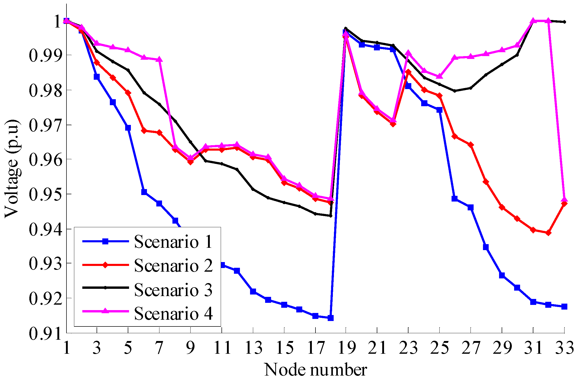
Figure 6.
The topology of solution of Scenario IV.
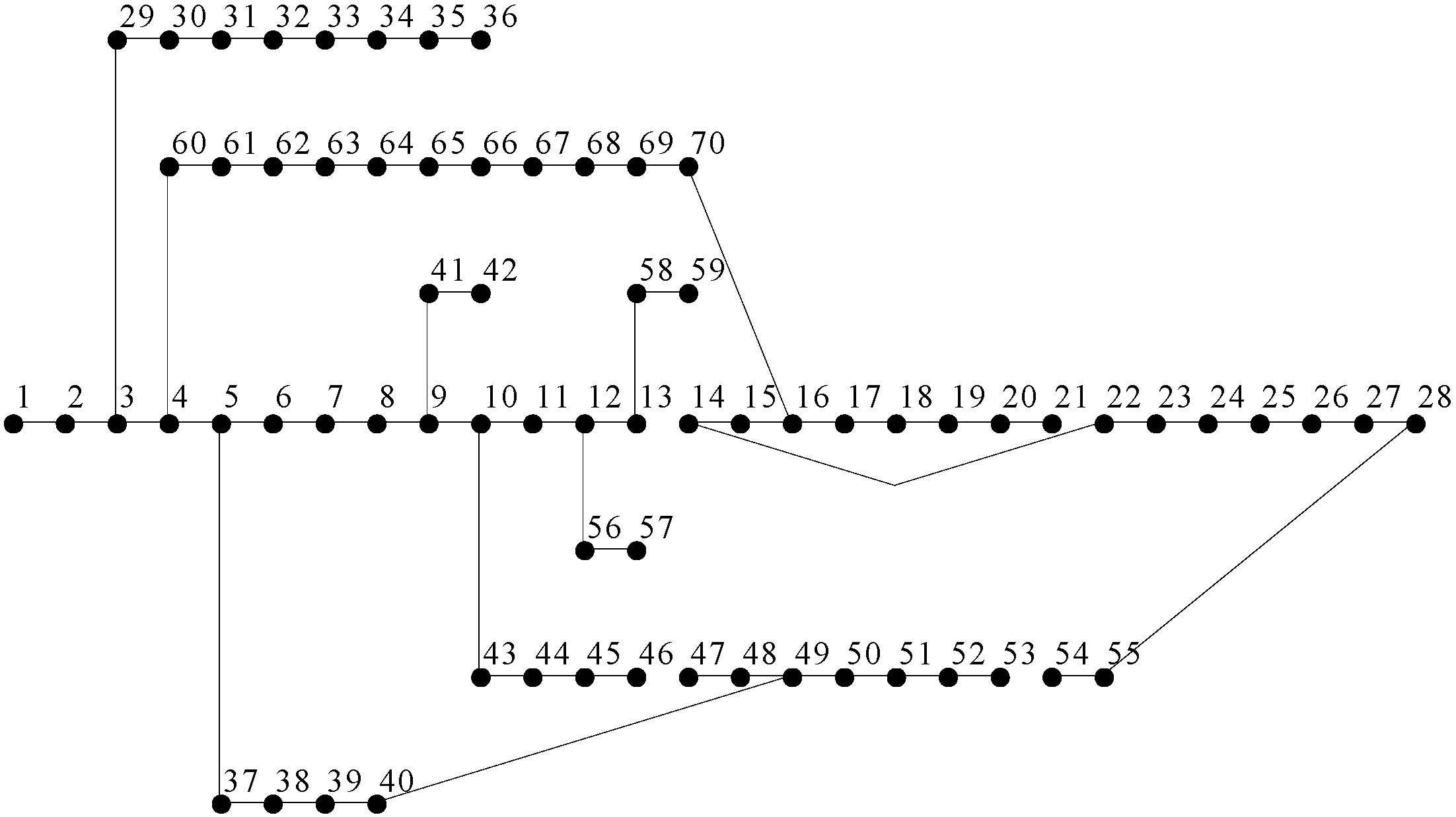
Figure 7.
Voltage profiles of PG&E 69-bus system.

Table 1.
Reliability data of related equipment (with interval data).
| Items | |
|---|---|
| Overhead Lines | 0.325 [0.292, 0.358] |
| Breaker | 0.0464 [0.0418, 0.0509] |
| Switch | 0.04 [0.036, 0.044] |
Table 2.
The optimization result of IEEE 33-bus system.
| Scenarios | Parameters (with Interval) | ||
|---|---|---|---|
| I | Open switches | {8–21, 9–15, 12–22, 18–33, 25–29} | |
| Power loss (kW) | 190.99 | [108.95, 266.06] | |
| EENS | 2709.4 | [2438.5, 2980.3] | |
| Minimum voltage (p.u.) | 0.9141 | [0.8719, 0.9178] | |
| II | Open switches | {7–8, 9–10, 14–15, 25–29, 32–33} | |
| Power loss (kW) | 129.83 (32.02%) | [75.41, 161.33] | |
| EENS | 2694.5 (0.6%) | [2425.1, 2964.5] | |
| Minimum voltage (p.u.) | 0.9388 | [0.9292, 0.9536] | |
| Operation number | 4 | ||
| Calculation time (s) | 16.54 | 21.95 | |
| III | Open switches | {8–21, 9–15, 12–22, 18–33, 25–29} | |
| DG Output & locations | DG1: 0.2364 kW, node 32 | ||
| DG2: 1.1652 kW, node 31 | |||
| Power loss (kW) | 68.54 (64.11%) | ||
| EENS | 2709.4 | ||
| Minimum voltage (p.u.) | 0.9438 | ||
| Calculation time (s) | 16.33 | ||
| IV | Open switches | {7–8, 9–10, 14–15, 25–29, 32–33} | |
| DG output & locations | DG1: 0.1511 kW, node 32 | ||
| DG2: 0.9057 kW, node 31 | |||
| Power loss (kW) | 63.80 (66.60%) | ||
| EENS | 2694.5 (0.6%) | ||
| Minimum voltage (p.u.) | 0.9482 | ||
| Operation number | 4 | ||
| Calculation time (s) | 30.08 | ||
Table 3.
The comparison of different methods in Scenarios II and IV.
| Items | Scenario II (Reduction for Crisp Data for Interval) | Scenario IV (Reduction) | |
|---|---|---|---|
| BPSO&HSA | 129.83 (32.02%) | [75.41, 161.33] (98.96%) | 63.80 (66.60%) |
| NSA | 143.20 (31.05%) | [84.20, 189.50] (97.20%) | N/A |
| HSA | 138.06 (31.88%) | N/A | 74.75 (63.12%) |
| HA | N/A | 45.00 (78.67%) | |
| CYMDIST | 135.52 (31.34%) | N/A | N/A |
Table 4.
The optimization result of PG&E 69-bus system.
| Scenario | Parameters (with Interval) | ||
|---|---|---|---|
| I | Open switches | {12–67, 14–22, 16–70, 40–49, 28–55} | |
| Power loss (kW) | 226.07 | [158.94, 307.69] | |
| EENS | 5094.0 | [4584.6, 5603.4] | |
| Minimum voltage (p.u.) | 0.9090 | [0.8937, 0.9238] | |
| II | Open switches | {13–14, 21–22, 46–47, 53–54, 12–67} | |
| Power loss (kW) | 102.54 | [72.94, 137.82] | |
| EENS | 4102.6 | [3692.4, 4512.9] | |
| Minimum voltage (p.u.) | 0.9466 | [0.9318, 0.9506] | |
| Operation number | 4 | ||
| III | Open switches | {12–67, 14–22, 16–70, 40–49, 28–55} | |
| DG output & locations | DG1: 0.7227 kW, node 51 | ||
| DG2: 0.8623 kW, node 54 | |||
| DG3: 0.2936 kW, node 48 | |||
| Power loss (kW) | 23.29 (89.70%) | ||
| EENS | 5094.0 | ||
| Minimum voltage (p.u.) | 0.9679 | ||
| IV | Open switches | {13–14, 21–22, 46–47, 53–54, 12–67} | |
| DG output & locations | DG1: 0.4709 kW, node 51 | ||
| DG2: 1.3517 kW, node 54 | |||
| DG3: 0.1966 kW, node 48 | |||
| Power loss (kW) | 10.78 | ||
| EENS | 4102.6 | ||
| Minimum voltage (p.u.) | 0.9902 | ||
| Operation number | 4 | ||
| Calculation time (s) | 42.28 | ||
Table 5.
Comparison of BPSO results under different settings in Scenario II.
| Population/Iteration | 600/30 | 400/30 | 600/20 | 400/20 | 1000/30 | 600/40 |
|---|---|---|---|---|---|---|
| Total time (s) | 41.80 | 36.76 | 29.45 | 23.51 | 50.78 | 57.03 |
| Function value (×103) | 446.04 | 472.62 | 481.45 | 509.30 | 446.04 | 446.04 |
Table 6.
Comparison of HSA results under different settings in Scenario III.
| HMS/NI | 6/5000 | 10/5000 | 4/5000 | 6/500 | 6/2000 | 6/10,000 |
|---|---|---|---|---|---|---|
| Total time (s) | 17.44 | 18.85 | 16.60 | 3.54 | 9.92 | 31.17 |
| Power loss (kW) | 23.29 | 23.28 | 23.31 | 24.37 | 23.58 | 23.29 |
The result is an average value of 5 repeated tests.
© 2017 by the authors. Licensee MDPI, Basel, Switzerland. This article is an open access article distributed under the terms and conditions of the Creative Commons Attribution (CC BY) license (http://creativecommons.org/licenses/by/4.0/).
Share and Cite
MDPI and ACS Style
Liu, K.-y.; Sheng, W.; Liu, Y.; Meng, X. A Network Reconfiguration Method Considering Data Uncertainties in Smart Distribution Networks. Energies 2017, 10, 618. https://doi.org/10.3390/en10050618
AMA Style
Liu K-y, Sheng W, Liu Y, Meng X. A Network Reconfiguration Method Considering Data Uncertainties in Smart Distribution Networks. Energies. 2017; 10(5):618. https://doi.org/10.3390/en10050618
Chicago/Turabian StyleLiu, Ke-yan, Wanxing Sheng, Yongmei Liu, and Xiaoli Meng. 2017. "A Network Reconfiguration Method Considering Data Uncertainties in Smart Distribution Networks" Energies 10, no. 5: 618. https://doi.org/10.3390/en10050618
Note that from the first issue of 2016, this journal uses article numbers instead of page numbers. See further details here.