Article

Evaluation Method for Real-Time Dynamic Line Ratings Based on Line Current Variation Model for Representing Forecast Error of Intermittent Renewable Generation

by
Hideharu Sugihara
1,*,
Tsuyoshi Funaki
1 and
Nobuyuki Yamaguchi
2
1
Division of Electrical, Electronic and Information Engineering, Graduate School of Engineering, Osaka University, Suita 565-0871, Japan
2
Department of Electrical Engineering, Faculty of Engineering Division, Tokyo University of Science, Tokyo 125-8585, Japan
*
Author to whom correspondence should be addressed.
Energies 2017, 10(4), 503; https://doi.org/10.3390/en10040503
Submission received: 7 February 2017 / Revised: 18 March 2017 / Accepted: 4 April 2017 / Published: 8 April 2017
(This article belongs to the Section F: Electrical Engineering)

Abstract

:
Due the high penetration of intermittent renewable energy sources (IRESs), transmission line currents show large fluctuations and thus significant uncertainty. This makes it difficult to operate a power system without violating transmission capacity constraints. This paper evaluates the dynamic line ratings (DLRs) of overhead lines based on changes in the line current owing to the high penetration of intermittent renewable energy sources. In particular, by focusing on extremely large (but rare) forecasting errors in the intermittent renewable energy source output, which are generally inevitable in most forecasting methods, a model for representing the forecasting error in line with current variation due to intermittent renewable energy source output is developed. The model is based on a shape parameter that represents the equivalent current variation required for the same temperature increase as that due to the extremely large forecasting error. Finally, based on the annual minute-by-minute irradiance data, preventive control of the transmission network with dynamic line ratings is evaluated using worst-case parameter values.

1. Introduction

Electric power generation from intermittent renewable energy sources (IRESs), including photovoltaic (PV) systems and wind power generators, exhibits significant output fluctuations. Given the increased penetration of IRESs, these output fluctuations may cause large power flow variations in transmission lines. Moreover, in addition to increased variability, it is very difficult to predict the output of IRESs accurately. Various methods for predicting IRES output have been developed using different time scales, spatial scales, and procedures [1,2,3,4,5,6]. In all these methods, it is critical to ensure the secure operation of power systems with IRESs. However, it has been noted that the distribution of the forecasting error is a heavy-tailed one instead of a normal one [7,8]. Therefore, even in the case of short-term predictions (e.g., those for less than 30 min) [9], extremely large forecasting errors must be considered during the operation of power systems, even though such errors occur rarely. Consequently, the planning and operation of such power systems can become less efficient even though their security levels are improved.
On the other hand, the capacity of overhead transmission lines is fundamentally determined by the temperature limit of the line conductor and not by the line current or the apparent power limit. Such temperature-based transmission capacity constraints are called dynamic line ratings (DLRs) [10,11]. Given recent advances in information and communication technology (ICT) and computational techniques (e.g., those used for meteorological predictions), real-time monitoring and forecasting technologies [12,13] might become available for DLR in the future. Although DLR was proposed several decades ago [10,11], the possibility and practicality of employing DLR [14,15,16] in the real-time operation of power systems have arisen only recently.
There have been numerous studies on DLR from a power system operations viewpoint. For instance, while taking into account future uncertainties in weather conditions, a robust economic dispatching method was proposed, based on both centralized and decentralized approaches [17]. Further, given the uncertainties related to wind power, a weather-based optimal power flow has been proposed [18]. However, these studies have tended to essentially focus on a single interval (snap shot) in the future. On the other hand, the DLR has been considered in unit commitment with security constraints of a transmission line fault [19]. From a practical power system operation viewpoint, the adaptive transmission capacity is evaluated based on the lead-time for control actions for alleviating the transmission line overload [20]. Reference [21] proposed a method for incorporating DLR with real-time weather conditions into existing system integrity protection schemes. Reference [22] evaluated the effect of DLR under assumed contingencies (N-1 and N-2 criteria) in a power system with high wind power penetration. However, almost all such studies have focused on the step-change in the transmission line current owing to the clearing of transmission line faults. A probabilistic modelling and simulation method for line temperature was developed based on Monte Carlo simulations while assuming the penetration of renewable energy sources [23]. However, this method does not explicitly consider the forecasting error (in particular, extremely large forecasting errors). Further, it requires additional computational resources because of the Monte Carlo simulation. From a practical viewpoint, a simpler and less computationally intensive model is needed for power system operation and control.
In general, in most transmission line wires used widely, the time constant at which the line conductor temperature changes is approximately 10–15 min; this is because of the thermal inertias of the line conductors [24]. In conventional power systems, the clearing of a transmission line fault is considered to result in a significant change in the line current within the short time involved (10–15 min). Consequently, in present power systems, the line protection schemes used for alleviating transmission line overloads focus on line fault clearing [21]. However, when the penetration of IRESs is high, the transmission line current fluctuates significantly and does not change in a step-like manner. In particular, among a wide variety of DLRs, electro-thermal coordination is the term covering the operation and planning of transmission systems based on temperature instead of current [25], rather than changes in the ambient meteorological parameters.
Further, it is important to model the variations in the line current caused by extremely large forecasting errors in IRES output. For such models, it is necessary to operate power systems such as one that is able to predict the rise in line temperature owing to extremely large forecasting errors. In particular, it is necessary to determine the variations in the line current in short time intervals (e.g., intervals of 1 min) in order to simulate the line conductor temperature accurately. However, most forecasting methods developed for IRESs are designed to generate outputs at a single time point or instance in the future. Therefore, a continuous-time model that can be used to perform accurate simulations for the desired time interval must be developed.
This paper proposes an evaluation method of DLR based on a continuous-time line current variation model for representing extremely large forecasting errors in IRES output in order to estimate the rise in line temperature accurately, assuming that the transmission line current fluctuates significantly because of the high penetration of IRESs. Moreover, a method for determining the shape parameter that represents the variation in the equivalent current for the continuous-time model based on long-term historical PV output data is developed. A persistent model is used for short-term forecasting (5, 10, 15, and 20 min ahead) of PV output. A quantitative analysis is performed on the forecasting error, and the shape parameter is determined based on the worst-case forecasting error. Using this shape parameter, the effect of the DLR is evaluated and compared to that of the conventional current-based line capacity case.

2. Simulation Model for Line Temperature

2.1. Steady-State Model

Conventionally, the rated current (continuously allowable current limit) is determined based on the steady-state conditions of line current and weather conditions, including the ambient temperature, solar irradiation, wind speed, and wind direction [26,27,28]. For calculating the maximum continuously allowable current limit in most countries, weather conditions are adopted based on the worst-case historical weather condition data. Under the above conditions, the continuously allowable current limit is determined on the basis of the following heat balance equation:
I2Rac × 10−5 + qs = qr + qC
where I is the current (A), Rac is the AC resistance (Ω/km), qs is the heat gain from solar radiation (W/cm), qr is the radiative cooling (W/cm), and qC is the convective cooling (W/cm).
The left hand side refers to the heated components, which represent internal resistive joule loss and solar heat gain. The right hand side refers to the cooling components, which represent convective cooling and radiative cooling. These four components are described in detail in Appendix A. Assuming steady-state conditions, the maximum continuous current limit can be determined by the heat balance equation.

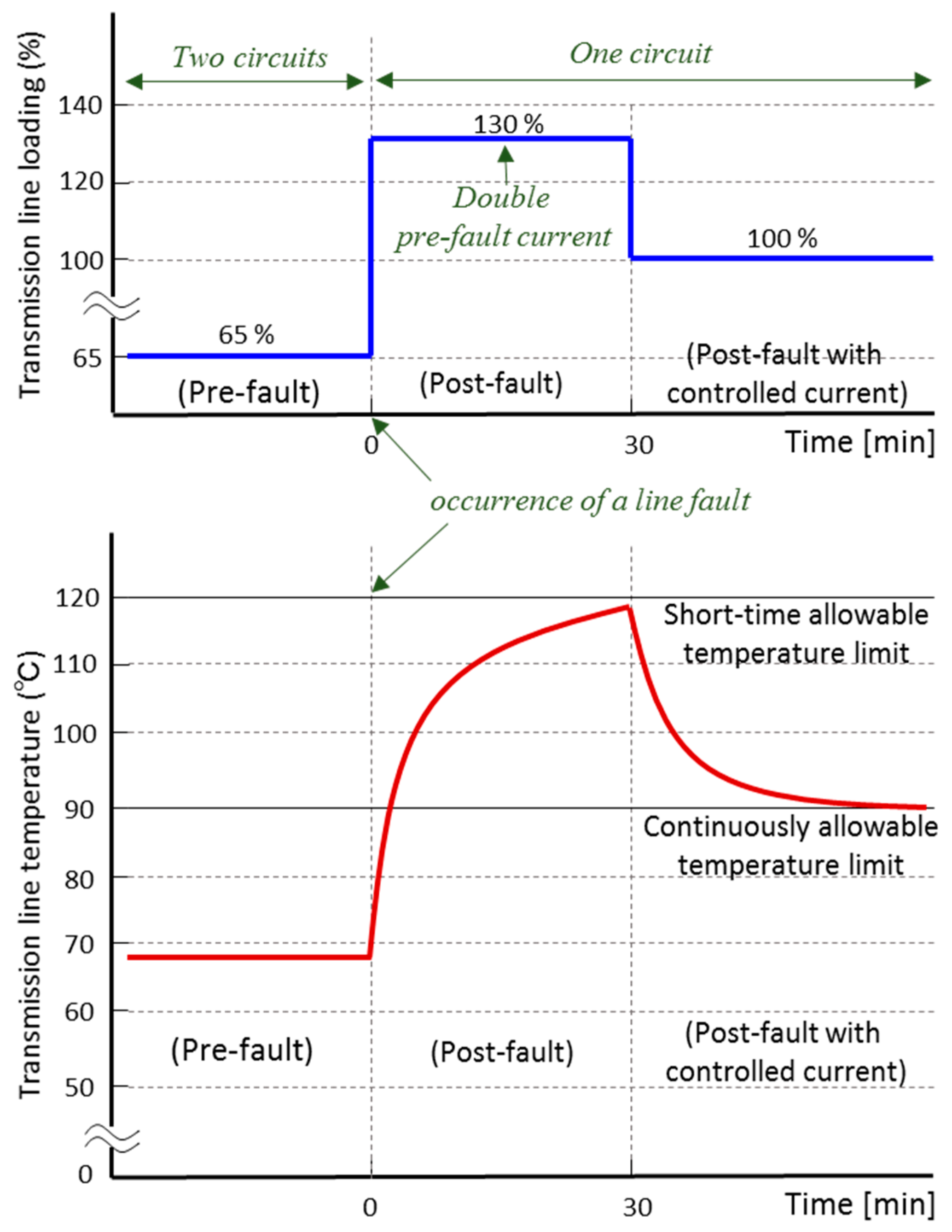
2.2. Transient-State Model

On the other hand, for high penetration of intermittent renewable energy resources, the line current also greatly fluctuates from a short-term system operational point of view. Therefore, it is necessary to consider a transient state of line conductor temperature. The line temperature at transient state conditions can be calculated using the following thermal model of the conductor:
d θ d t = ( R a c ( θ ) I 2 × 10 5 + q s ) ( q r ( θ ) + q c ( θ ) ) C ,
where θ is the temperature difference between the conductor and the ambient surroundings and C is the heat capacity of the line conductor (J/(cm·°C)).
As a simple method for solving the above first-order ordinary differential equation (Equation (2)), the modified Euler’s method is used in this study. In general, the ambient meteorological conditions have a significant impact on the line temperature (i.e., θ). However, because this paper focuses on the change in line current due to the extremely large forecasting error of IRES, those meteorological parameters are assumed as conventional worst-case conditions. For further development, the proposed line current model explained in the following section can be utilized in arbitrary meteorological conditions if we can identify accurate meteorological parameters.

3. Continuous-Time Forecasting Error Model for Renewable Energy Output

3.1. Conventional Step Change in Line Current

In conventional power system operation, the short-term allowable current limit is determined by simulating the increase in line temperature while assuming a step-change in the current owing to a transmission line fault (N-1 criterion), as shown in Figure 1. This figure assumes that, as the most common case, one of the two circuits is disconnected owing to the clearing of a transmission line fault. As a result, after the transmission line fault has been cleared, the line current is temporarily doubled. Consequently, the transmission line temperature in the non-fault circuit increases based on the thermal inertia of the line conductor (i.e., as in Equation (2)). At this time, if the condition of the line wire allows, the short-time allowable temperature limit can be allowed to rise until 120 °C is reached, which is higher than the continuously allowable temperature limit (90 °C). This increase in the temperature limit causes the wires to degrade. Therefore, the line temperature limit is assumed to be a continuously permissible current limit in this paper. However, the proposed line current variation model can be readily applied in the case of other temperature limits as well.
Further, in this figure, it is assumed that a control action for line overload relief from 130% to 100% (e.g., generation re-dispatch, load shedding, or any other such action) can be taken at, for instance, 30 min after a transmission line fault. Consequently, the transmission line conductor temperature is reduced immediately. Finally, in conventional N-1-based operation, the line current limit under normal operating conditions is determined based on a similar preventive control viewpoint.

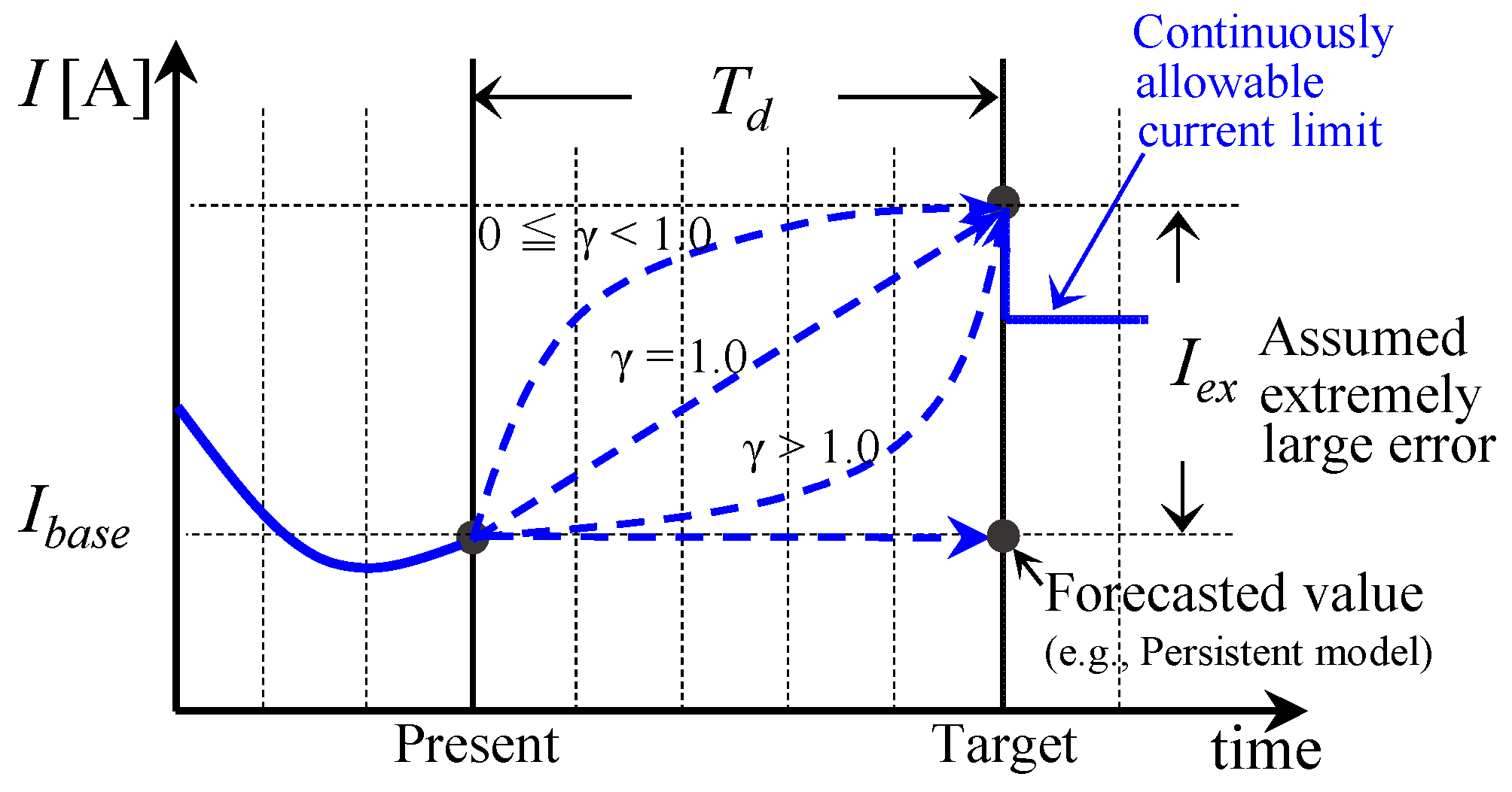
3.2. Proposed Line Current Variation Model for Representing Extremely Large Forecasting Errors

This paper focuses on transmission line overloads caused by extremely large but rare forecasting errors in the line current. In such cases, the change in the transmission line current is markedly different from a step change in the current. Moreover, most forecasting methods can usually make predictions for a single (or several discrete) future time interval(s) (e.g., for 15 min ahead). Consequently, the line current profiles for the present time and the target time horizon may not usually be specified. However, in order to simulate the line conductor temperature accurately, it is essential to consider the change in the line current at intervals of at least 1 min. A continuous-time model for large forecasting errors is better suited for evaluating the line temperature with precision.
From a practical viewpoint, for extremely large forecasting errors, a number of different profiles exist for the change in line current. However, the line temperature profile and, in particular, the maximum temperature corresponding to extremely large errors are more important than that for the estimated line current because the former affects the lifetime of the line conductor. Therefore, in this paper, we propose an equivalent change in the line current that can result in the same temperature increase as those caused by extremely large forecasting errors. The continuous-time model for extremely large forecasting errors shown in Figure 2 can be developed as:
I ( t ) = I e x ( t T d ) γ + I b a s e ,
where Iex is the assumed extremely large forecasting error at the target point in time, Td is the lead-time for a control action, Ibase is the current at the present time, γ is the shape parameter, and t is time.
In Equation (3), γ is the most important parameter and represents the severity of the curve, as shown in Figure 2. Further, Td, Ibase, and Iex are the forecasting lead-time for a control action, the forecasted current value, and the assumed large forecasting error in Figure 2, respectively. These three values are exogenous parameters in this analysis. Ibase and Iex are determined using a forecasting method that is usually based on a persistent model for very short-term predictions (e.g., within 30 min) for renewable energy generation. Td is the time interval between the present time and the target time in Figure 2 and corresponds to the interval from 0 to 30 min in Figure 1.
One advantage of this model is that only one parameter (γ) is used for simulating the temperature increase of the transmission line due to the extremely large forecasting error. In particular, the line temperature within the target period increases monotonically as the shape parameter (γ) is reduced. Further, the physical meaning of the shape parameter is that a value of 1 indicates linear interpolation, while a value of 0 indicates that the approaching step-changed current, which is approximated by a time interval, depends on the length of the time interval (e.g., 1 min).

3.3. Method for Determining the Shape Parameter γ

Although the real time application of preventive control using γ is proposed in this study, the appropriate value of worst-case γ is determined by the off-line analysis of historical line current data. In order to achieve that, we first calculate the line temperature in advance, using historical line current data off-line. Consequently, using the line conductor temperature after Td min, we can evaluate the appropriate value of γ, which represents the increase in the line temperature after Td min, relative to the present temperature of the conductor.
When determining the value of the shape parameter, the line temperature is always more significant with respect to permanent damage in the line wire. Therefore, the parameter γ is determined so that the line temperature rises by the same amount as the increase caused by large forecasting errors. Consequently, the equivalent variation in the line current can be obtained by adjusting the shape parameter γ. In the simulation described later in this paper, in order to analyze the fundamental characteristics of the proposed line current variation model, Iex and Td are changed on the basis of sensitivity analysis.

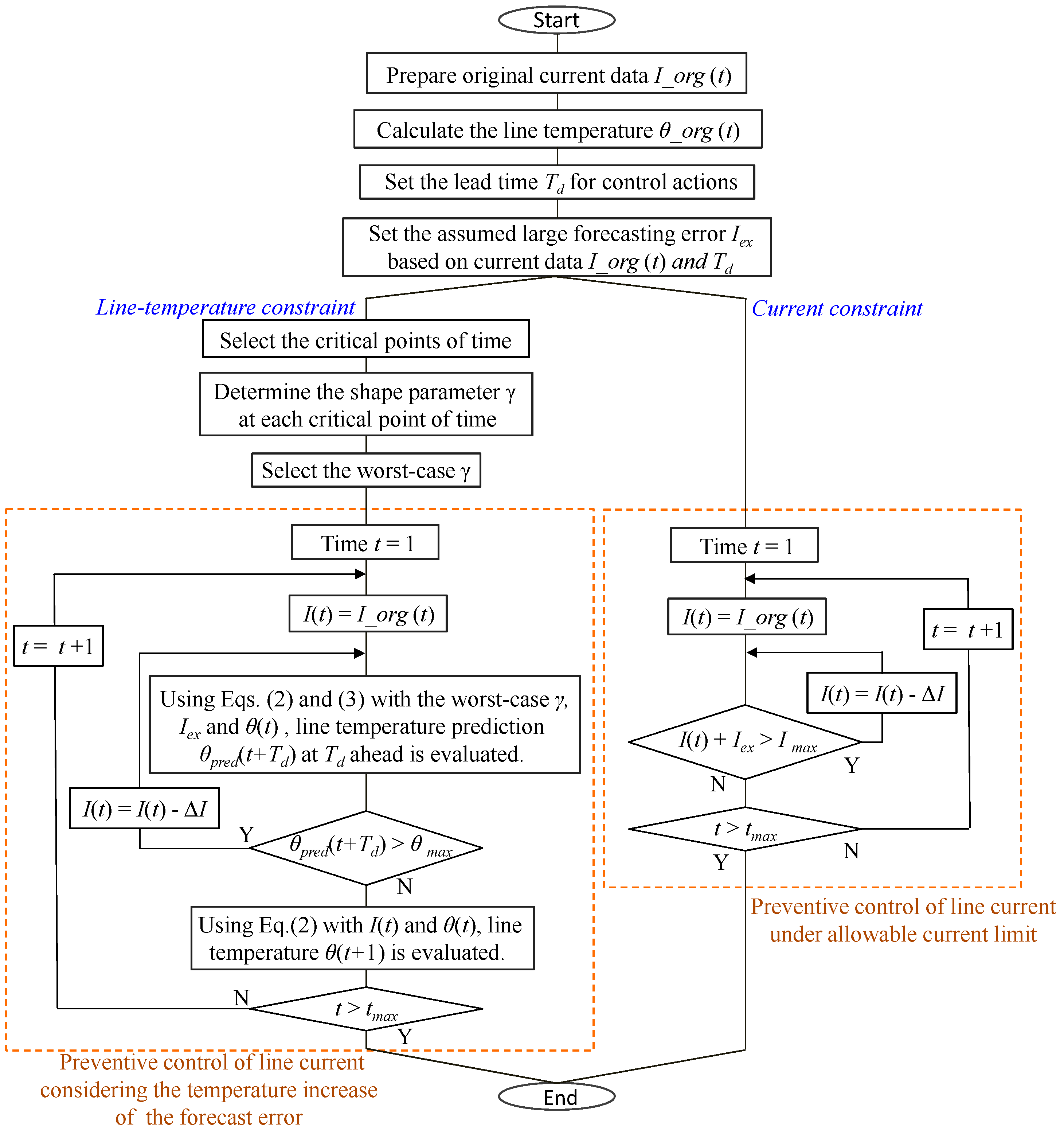
3.4. Flowchart for Long-Term Evaluation from a Preventive Control Viewpoint

A flowchart is shown in Figure 3 for evaluating the benefits of DLR using the proposed model. This figure shows the procedure for evaluating the temperature-based transmission capacity constraints using the proposed model for forecasting errors in the IRES output while comparing it with the conventional current-based transmission capacity. Before starting the simulation, the line current I_org(t) and the corresponding line temperature θ_org(t) are calculated in advance based on Equation (2). Next, the lead-time Td for the control action and the forecasting error in the current I_org(t), which is determined using a forecasting method, at the time interval Td are calculated. The persistent method, which is used in the simulation that follows, is one of most effective forecasting methods for very short-term intervals (30 min or less).
Next, in the case of the temperature-based transmission capacity (i.e., DLR), the forecasting error for the line current is significant with respect to the transmission line temperature limit when the temperature is relatively high. Therefore, we assume that the significant points of time corresponding to both high temperature and large forecasting error need to be selected. Then, the appropriate value of γ is determined at each point in time. Using the minimum value of γ as the worst-case value, we can then simulate the preventive control action in the case of temperature-based transmission capacity. In particular, at simulation time instant t, we assume that line current I(t) is initially set to original current I_org(t). Using the worst-case γ and the assumed forecasting error Iex, a predicted line temperature θpred(t + Td) can be calculated using the proposed model. Until the predicted line temperature at Td (min) later is lower than the maximum allowable temperature limit θmax, the line current I(t) must be reduced. Once the predicted line temperature θpred(t + Td) becomes lower than the maximum allowable temperature limit, the line temperature θ(t + 1) can be determined using the line current I(t) and the previous line temperature θ(t).
As a comparative case, the preventive control action with respect to conventional current-based transmission capacity is evaluated using the control lead-time Td and the assumed forecasting error Iex at the lead-time. More specifically, at simulation time instant t, we assume that line current I(t) is initially set to original current I_org(t). Until the predicted line current at Td (min) later is lower than the maximum allowable current limit Imax, the line current I(t) must be reduced. Next, the line current I(t) can be determined. We then compare the two cases corresponding to the temperature-based transmission capacity and the conventional current-based capacity for the same forecasting error Iex.

4. Simulation Evaluation

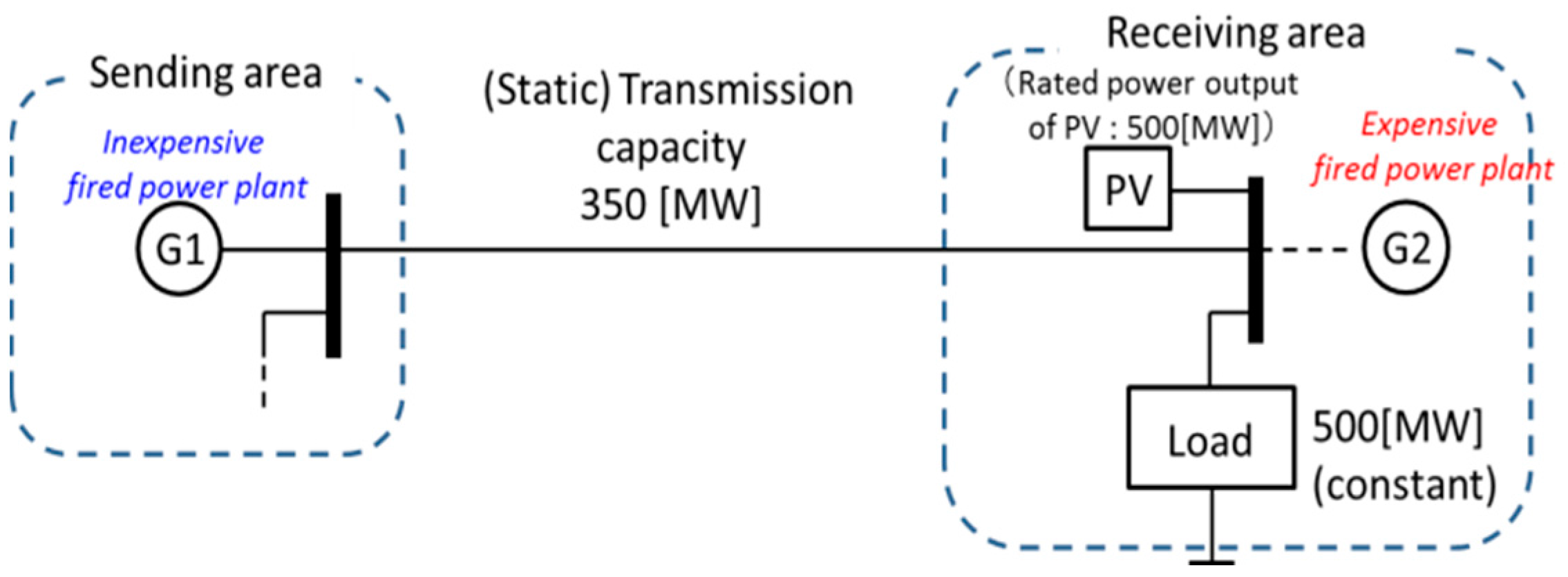
4.1. Simulation Conditions

In many cases, large-scale PV plants or wind farms are connected to buses in sub-transmission or distribution networks. The line capacity overload problem first occurs in the networks when PV plants or wind farms are connected to a bus intensively. Consequently, this paper focuses on the radial network topology that is adopted in sub-transmission and distribution networks in some countries (including Japan [29,30]).
In the radial network topology, it is comparatively easy to identify the relationship between the line current variation and the forecasting error of renewable energy sources. In order to analyze the fundamental characteristics of the line current variation model with line-temperature constraints, this paper uses a simple two-bus test system [25], as shown in Figure 4. The simulation analysis was performed for daytime (e.g., from 10:00 to 14:00), and the load in the receiving bus during daytime was assumed to be constant in order to keep the transmission line current constant in the absence of a PV system. Actual monitored solar irradiation data (minute by minute) for Osaka, Japan, were used to generate the fluctuation in the output power of the PV system. We considered the spatial smoothing effect of the solar irradiation data based on the transfer hypothesis [31,32]. Moreover, based on this hypothesis, we have analyzed the effect of spatial smoothing on the variation in line temperature; this paper adopted Case B (where the area is 100 km2) in [33]. In the test system, the transmission line current from the sending bus to the receiving bus also fluctuated in order to compensate for the PV output fluctuations. The line conductor was assumed to be ACSR (Aluminium Conductors Steel Reinforced) wire (160 mm2). The continuously allowable temperature and current were 90 °C and 465 A, respectively. The ambient weather conditions were taken as worst-case conditions, which are widely used in Japan, as shown in Table 1.
In this paper, as the weather parameter is assumed as the worst-case condition in Table 1, the calculated temperature of line conductor based on the worst-case conditions is higher than the (unknown) real temperature of the line conductor. In present power systems, the line temperature based on the worst-case conditions would be acceptable as a conservative evaluation for system operators. In a future power system, a more realistic temperature of the line conductor can be calculated if the real-time monitoring system for meteorological parameters can be utilized, particularly in a critical line corridor. Consequently, the proposed line current variation model can be applied more appropriately to the DLR environment with realistic weather conditions. The evaluation of when to utilize the real-time monitoring system of meteorological parameters is part of further developments.
In future power systems, the wide deployment of demand response resources is necessary to install many large-scale intermittent renewable energy resources [34,35]. Therefore, we focused on the demand response as a control action for alleviating transmission line overloads. In the model of the demand response, the control delay Td of the demand response was an important parameter; its values were taken to be 5 min, 10 min, 15 min, and 20 min. For example, the ‘responsive reserve’ in ERCOT (the Electric Reliability Council of Texas) must reduce the demand within 10 min after control signals are received [36]. In present power system operations, it might be difficult to control a large amount of electricity demand within a short period of time from a customer convenience point of view. However, as a special case of rapid load curtailment in some utilities, there are some direct load controls for air-conditioners [37], water heaters [38], etc. Moreover, as a promising, fast, and responsible equipment in future environments, customer-owned battery storage systems [39] might be useful for rapid responses.

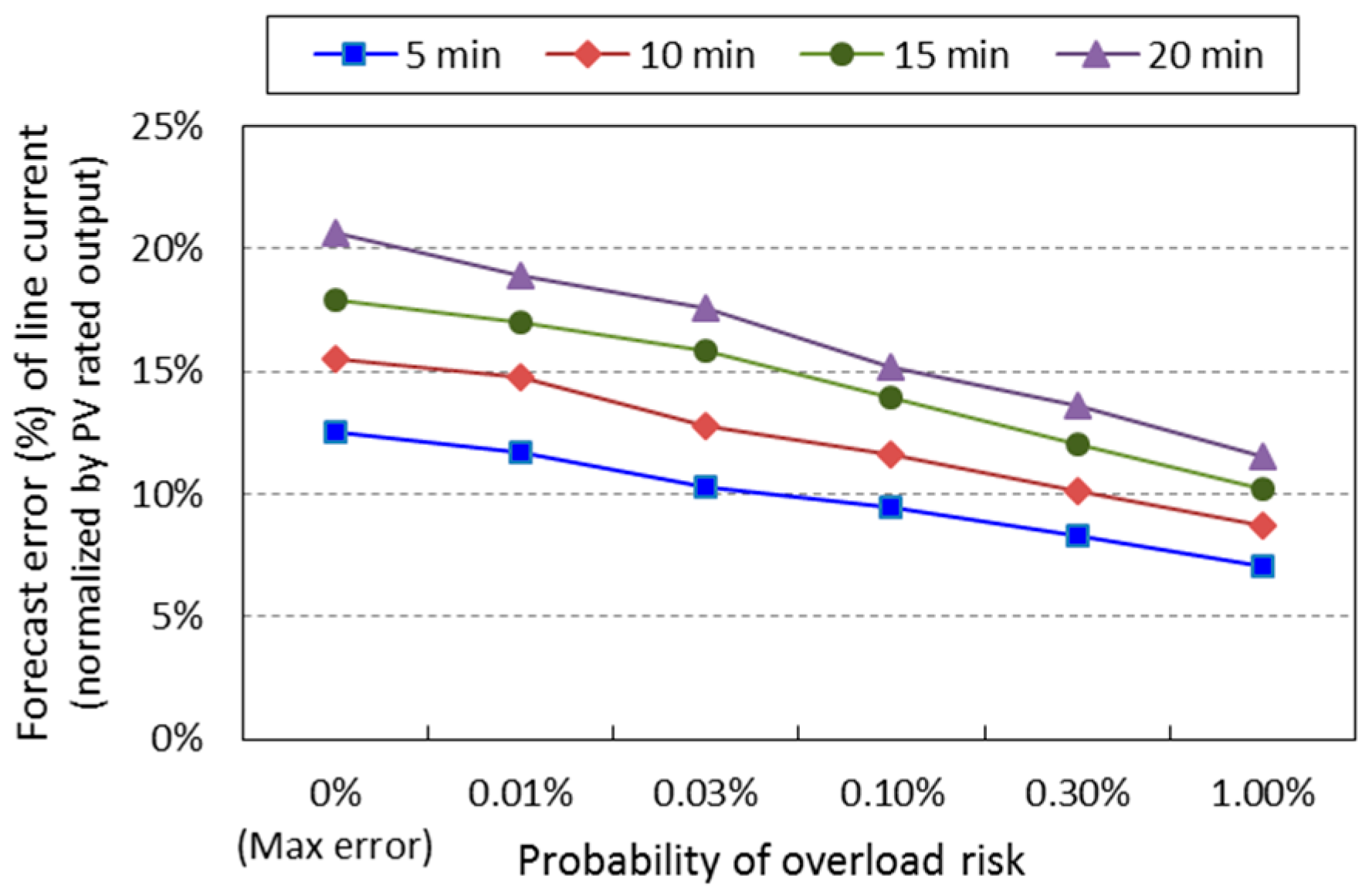
4.2. Evaluation of Forecasting Error

When using the line current variation model shown in Figure 2, the assumed forecasting error Iex at the target time interval Td can be considered an exogenous parameter. In this paper, by adopting the persistent model, the forecasting error for the transmission line current for four different lead-times (5 min, 10 min, 15 min, and 20 min) for a fast demand response was evaluated from an annual viewpoint. Based on the annual forecasting error data for the four different lead-times, the overload risk of Iex was evaluated as shown in Figure 5. As stated at the simulation condition (Section 4.1, assuming that load current between the sending area and the receiving area was constant, line current forecasting error was normalized by PV rated capacity as shown in the figure.
The horizontal axis in Figure 5 represents the risk of exceeding the forecasting error. Specifically, if Iex is set to the maximum forecasting error for each lead-time, the overload risk level is zero based on the annual forecasting error data. If Iex is smaller than the maximum error, the risk level for overload increases. Therefore, the assumed forecasting error, Iex, in Equation (3) was related to the overload risk level, which can be regarded as a system operational policy.

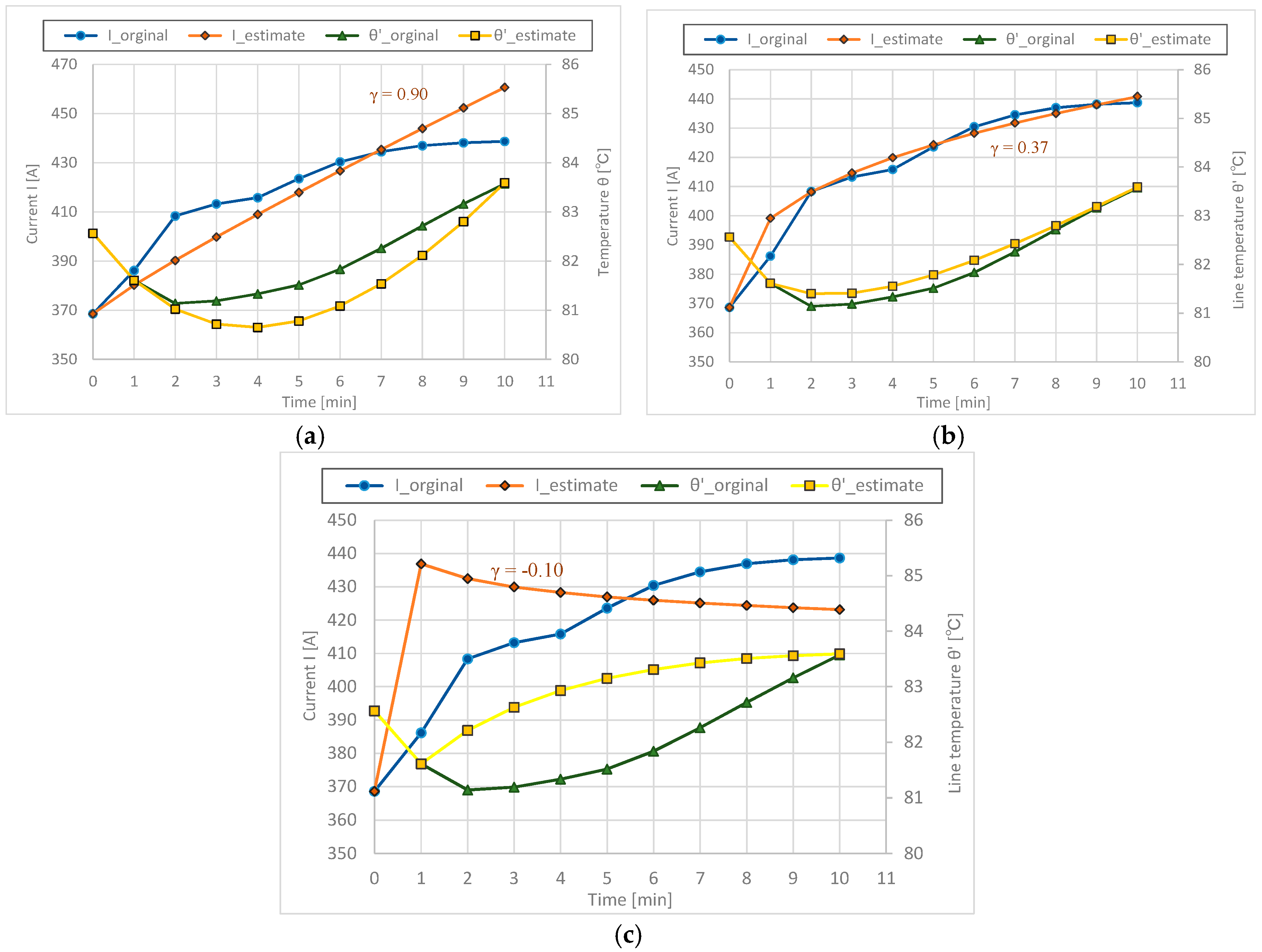
4.3. Evaluation of Shape Parameter γ

Although it is possible to calculate γ for each time instance (that is, on a minute-by-minute basis) based on the annual data, such calculations would be meaningless most of the time. Therefore, in order to determine the shape parameter γ, a few points in time were selected from the viewpoints of both high conductor temperature and large line current forecasting error. From a preventive control viewpoint with respect to power system operations, the worst-case value (i.e., the minimum value) of γ is the most extreme for simulating the transmission line overload problem. Thus, as the criterion for selecting a few significant time points from the historical data, we assumed that the line temperature was higher than 82 °C (90 °C is the continuously allowable temperature limit) and that the forecasting error in the line current was larger than 40 A (465 A is the continuously allowable current limit). The number of target time points is listed in Table 2. Depending on the lead-time for the control action (5 min, 10 min, 15 min, and 20 min), the number of target time points selected from the annual data were 4, 26, 65, and 139, respectively.
Furthermore, the minimum and maximum values of γ are also shown for each case in Table 2. As the probability (risk) of exceeding the forecasting error, which is a fundamental characteristic, becomes larger, the minimum and maximum values of γ both decrease because the forecasting error Iex decreases, as shown in Figure 5. Consequently, the γ value decreases in order to reach the increase required in the line conductor temperature for each forecasting lead-time. Furthermore, as Td increases, the minimum and maximum values of γ both increase because the change in the line current increases gradually.
The value of γ is negative in the worst case where the probability (risk) is the highest (1.0%). In order to illustrate this case, while focusing on the case corresponding to a lead-time Td of 10 min, a few examples with different probabilities (0.01%, 0.10%, and 1.00%) are shown in Figure 6. In Figure 6a, it is assumed that the forecasting error Iex at the target time is larger than the actual error. Therefore, in order to fit the estimated line temperature to the actual one, the appropriate γ value was determined and found to be 0.90. Further, in the case of a probability of 0.10%, Iex was smaller than 0.01%. Therefore, the appropriate γ was determined to be 0.37. Consequently, the current variation, as estimated using the proposed model, was close to the actual variation in the current. However, for a probability of 1.0%, the value of γ was slightly negative (−0.10) in order to fit to the actual line temperature at a subsequent 10-min interval because the Iex value was too small.

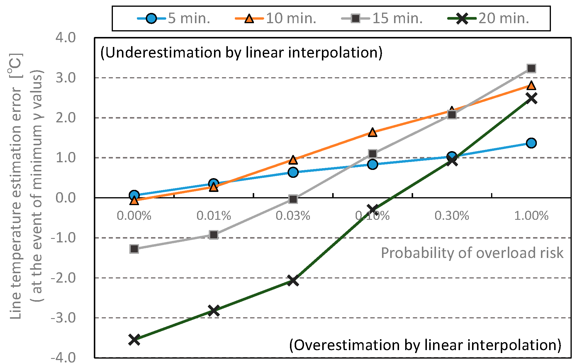
4.4. Comparison with Linear Interpolation

A simple linear interpolation of line current variation between line current at the existing time and at the forecasted time can help to comparatively understand the proposed line current variation model. Figure 7 shows the line temperature estimation error obtained using a simple linear interpolation (γ = 1) in the event of the respective minimum γ value in Table 2. In the figure, a positive error in line temperature implies an underestimation by linear interpolation, while a negative error indicates overestimation by linear interpolation. In Table 2, minimum γ values range from approximately 0.0 to 1.0 in the cases of 5 min and 10 min, respectively. Consequently, in Figure 7, an occurrence of underestimation by simple linear interpolation is shown. Furthermore, the estimation error for the 10 min case was larger than that for the 5-min case because the temperature estimation error was accumulated for the lead-time. In the cases of lead-times of 15 min and 20 min, the minimum γ values ranged from 1.42 to −0.08 and from 2.22 to 0.53, respectively (see Table 2). Consequently, in Figure 7, both overestimations and underestimations occur. Furthermore, similar to the 5-min and 10-min cases, the estimation error width of the 20-min case was larger than that of the 15-min case because the temperature estimation error accumulated. Considering the maximum allowable temperature limit (90 °C), those estimation errors are significant.

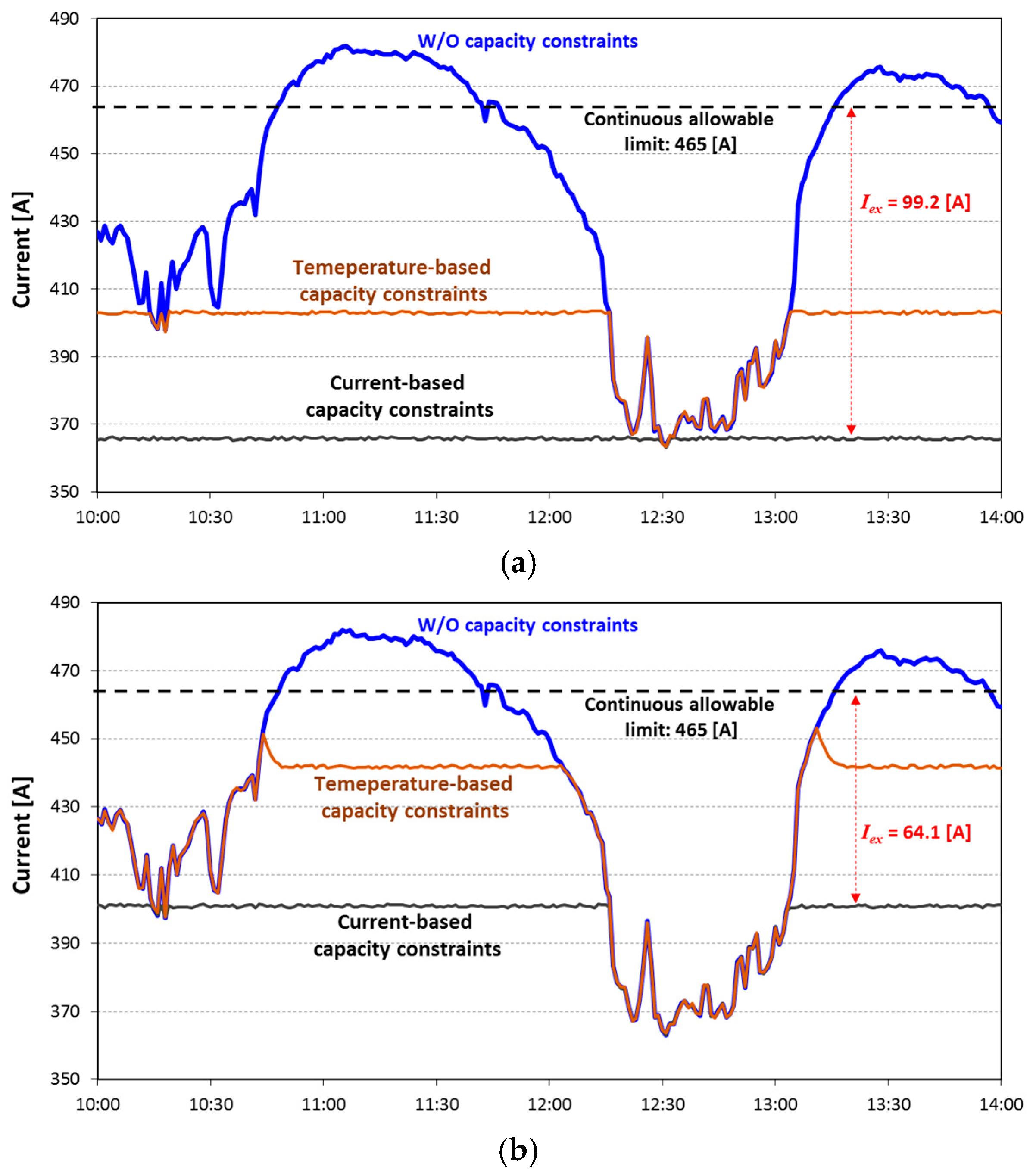
4.5. Simulation Results on a Sample Day

This section explains the effects of the temperature-based transmission capacity constraints for a sample day. As a simulation condition, this focused on 15-min-ahead and 5-min-ahead forecasts at the 0.03% risk level, as shown in Figure 8a,b, respectively. In case of the forecast for 15 min, according to Figure 5, Iex was comparatively larger (99.2 (A) corresponds to 15.9% PVrated). Therefore, in Figure 9a, the conventional current-based transmission capacity poses a lower line current limit. However, in the case of the temperature-based transmission capacity, although the same forecasting error (99.2 (A): 15.9% PVrated) was assumed, the line current changed slowly because the worst-case value of γ was 1.012. This led to a slow increase in the line conductor temperature. Consequently, the line current limit, which can be flown through the sub-transmission line from a preventive control perspective, was higher compared to the conventional current-based capacity constraints.
According to Figure 5, Iex in the case of the 5-min forecast was 64.1 (A) (equal to 10.3% PVrated) and smaller than that for the 15-min case. Therefore, in Figure 8b, the line current corresponding to the conventional current-based transmission capacity was larger than that for the 15-min case. In the case of the temperature-based transmission capacity, considering the time constant for the increase in the line temperature, the load control action could be taken before the line temperature began to plateau. As a result, the transmission line current for the assumed large forecasting error could be increased. Furthermore, as can be seen from Figure 8b, the line current could be increased temporarily instead of following the steady-state limit when a sharp increase occurred in the line current.

4.6. Simulation Results Using Annual Data

The temperature-based (i.e., dynamic line rating) and the conventional step-changed-current-based transmission capacities were compared based on annual data. Specifically, the load curtailment resulting from the real-time application of the temperature-based transmission capacity constraint to the annual minute-to-minute data was evaluated. The load was assumed to be constant. The irradiation data were from 10:00 to 14:00 for 365 days. In order to facilitate comparison of the two capacities, the reduction percentage in load curtailment based on the temperature-based transmission capacity was calculated as:
η = E A E B E A × 100 ( % ) ,
where EA is the reduction in energy due to the step-changed current-based constraints ((A·min)/year) and EB is the reduction in energy due to the temperature-based method (dynamic line rating) ((A·min)/year).
The simulation results are shown in Figure 9. For all lead-times, as the assumed risk level for overload decreased, the benefit of using the temperature-based transmission capacity instead of the conventional current-based transmission capacity became larger because the shape parameter γ increased. Conversely, as the assumed risk level for overload increased, the benefit of the temperature-based capacity decreased. Specifically, in this case, the temperature-based transmission capacity was almost same as the conventional current-based transmission capacity.
However, for the worst-case scenario, as shown in Figure 6, the probability was 0.10%, and the modeled change in the current was similar to the actual change in the line current. Therefore, for example, if the risk level (0.10%) was adopted as an appropriate parameter, the benefit of the temperature-based transmission capacity remained at 40% for three lead-times (10 min, 15 min, and 20 min). Further, in case of the 5-min lead-time, the benefit of the temperature-based transmission capacity was still larger even though the risk level had increased. Thus the temperature change did not start to plateau within 5 min because of the thermal inertia of the line conductor.

5. Discussion and Further Research

A more detailed model can be obtained if the actual data of the line current and line temperature are used directly as opposed to those used in the proposed current variation model. However, in addition to the fact that each occurrence of a large forecasting error results in a large amount of data, it is relatively difficult for system operators to compare such unforeseen and extremely rare events at different times and on different lines. By using the shape parameter (γ), the essential features can be characterized using the proposed model (Equation (3)) in the case of the forecasting method actually utilized. Consequently, these unforeseen and extremely rare events can be easily and comprehensively understood by system operators.
In addition, as an example, the proposed line current variation model can be applied to the problem described below. In a radial distribution network with a solidly grounded system or a resistance-grounded system, the optimal coordination of overcurrent protective relays is a serious problem that needs to be addressed in the case of the high penetration of distributed renewable (including PV) sources [40,41]. In this case, two parameters (the pickup current and the time multiplier setting) for the relay settings are determined under different system conditions based on inverse-time characteristics [42]. The output variations and forecasting errors related to renewable energy can be considered in the case of the optimal coordination of overcurrent relays.

6. Conclusions

The DLR of line conductor temperature based on conventional step-changed current had been evaluated in the past; however, with regard to the high penetration of IRESs in this paper, the authors proposed a line current variation model for representing the forecasting error of IRESs and evaluated the DLR from a real-time application viewpoint for preventative control actions using the model. In contrast to the case of the step-change current attributed to line contingencies, the variations in line current due to the forecasting error of IRESs could be represented with a shape parameter in the proposed model. Consequently, the extremely large forecasting error of IRES output can be characterized by using the shape parameter in the proposed model, unlike conventional and simple linear-interpolation for the forecasting error between the present time and the forecasted time.
Through numerical simulations, the characteristics of the shape parameter were analyzed while assuming that the persistent model was used for forecasting. The worst-case values of the shape parameter for various lead-times and risk levels ranged from zero to two. Using the worst-case value for the shape parameter, the real-time operation of the transmission system was evaluated from a preventive control viewpoint. For example, when a risk level of 0.10% was adopted as being suitable, the temperature-based transmission capacity was approximately 40% lower than the load curtailment for three of the lead-times (10 min, 15 min, and 20 min). For a lead-time of 5 min, the benefit of the temperature-based transmission capacity was even greater, resulting in an approximately 65% reduction in load curtailment.
Finally, this paper focused on the fundamental characteristics of the proposed continuous-time forecasting error model while assuming the worst-case ambient weather conditions. However, the evaluation can easily be extended to other ambient conditions as well if seasonal ambient conditions are used when determining the shape parameter γ.

Acknowledgments

This work was supported by JST CREST Grant Number JPMJCR15K1, Japan.

Author Contributions

Hideharu Sugihara conceived and constructed the evaluation methodology; Hideharu Sugihara programmed the code and performed the simulations; Hideharu Sugihara and Tsuyoshi Funaki wrote the paper; Hideharu Sugihara, Nobuyuki Yamaguchi, and Tsuyoshi Funaki discussed the simulation results and made the paper modification.

Conflicts of Interest

The authors declare no conflict of interest.

Appendix A

This paper adopts the International Council on Large Electric Systems (so-called CIGRE) model [26] in order to calculate the transmission line temperature. In the heat balance equation (Equation (2)), there are two heating components and two cooling components. In the heating components, AC resistance and solar heat gain can be expressed as follows:
R a c ( θ ) = β R d c { 1 + α ( T + θ 20 ) } ,
q s = W s d η a ,
where β is the AC/DC resistance ratio, Rdc is the DC resistance at 20 °C (Ω/km), α is the temperature coefficient of resistance, T is the ambient temperature (°C), Ws is the solar irradiation (W/cm2), d is the diameter (cm), and η a is the absorptivity.
On the other hand, calculations for the cooling components, namely the convective and radiative cooling components, can be done respectively as follows:
-
Radiative cooling (Stefan–Boltzman Law):
q r ( θ ) = η e π d θ h r ( θ ) .
h r ( θ ) = 0.000567 ( 273 + T + θ 100 ) 4 ( 273 + T 100 ) 4 θ .
-
Convective cooling (forced convection case: v 0.5 ( m / s ) ):
q c ( θ ) = π d θ h ( θ ) K φ .
h ( θ ) = ( 2.42 × 10 2 + 7.2 × 10 5 × θ + 2 T 2 ) × ( v × d × 10 2 × exp ( 1.16 × 10 4 × y ) 1.32 × 10 5 + θ + 2 T 2 9.5 × 10 8 ) 0.471 × 0.641 d × 10 2 ,
K φ = { 0.42 + 0.58 ( cos φ ) 0.9 ; ( 0 φ 66 ) 0.42 + 0.68 ( cos φ ) 1.08 ; ( 66 < φ 90 ) ,
where T is the ambient temperature (°C), η e is the emissivity, y is the elevation (m), v is the wind velocity (m/s), φ is the wind direction angle (deg), and d is the diameter (cm).

References

  1. Ssekulima, E.B.; Anwar, M.B.; Al Hinai, A.; El Moursi, M.S. Wind speed and solar irradiance forecasting techniques for enhanced renewable energy integration with the grid: A review. IET. Renew. Power Gener. 2016, 10, 885–898. [Google Scholar] [CrossRef]
  2. Inman, R.H.; Pedro, H.T.C.; Coimbra, C.F.M. Solar forecasting methods for renewable energy integration. Prog. Energy Combust. Sci. 2013, 39, 535–576. [Google Scholar] [CrossRef]
  3. Shao, H.; Wei, H.; Deng, X.; Xing, S. Short-term wind speed forecasting using wavelet transformation and AdaBoosting neural networks in Yunnan wind farm. IET. Renew. Power Gener. 2016. [Google Scholar] [CrossRef]
  4. Stephen, B.; Galloway, S.; McMillan, D.; Anderson, L.; Ault, G. Statistical profiling of site wind resource speed and directional characteristics. IET. Renew. Power Gener. 2013, 7, 583–592. [Google Scholar] [CrossRef]
  5. Chitsaz, H.; Amjady, N.; Zareipour, H. Wind power forecast using wavelet neural network trained by improved Clonal selection algorithm. Energy Convers. Manag. 2015, 89, 588–598. [Google Scholar] [CrossRef]
  6. Nijhuis, M.; Rawn, B.; Gibescu, M. Prediction of power fluctuation classes for photovoltaic installations and potential benefits of dynamic reserve allocation. IET. Renew. Power Gener. 2014, 8, 314–323. [Google Scholar] [CrossRef]
  7. Yang, C.; Thatte, A.A.; Xie, L. Multitime-scale data-driven spatio-temporal forecast of photovoltaic generation. IEEE Trans. Sustain. Energy 2015, 6, 104–112. [Google Scholar] [CrossRef]
  8. Golestaneh, F.; Pinson, P.; Gooi, H.B. Very short-term nonparametric probabilistic forecasting of renewable energy generation—With application to solar energy. IEEE Trans. Power Syst. 2016, 31, 3850–3863. [Google Scholar] [CrossRef]
  9. Ganger, D.; Zhang, J.; Vittal, V. Statistical characterization of wind power ramps via extreme value analysis. IEEE Trans. Power Syst. 2014, 29, 3118–3119. [Google Scholar] [CrossRef]
  10. Davis, M.W. A new thermal rating approach: The real time thermal rating system for strategic overhead conductor transmission lines—Part I: General description and justification of the real time thermal rating system. IEEE Trans. Power Appl. Syst. 1977, 96, 803–809. [Google Scholar] [CrossRef]
  11. Douglass, D.A.; Edris, A. Real-time monitoring and dynamic thermal rating of power transmission circuits. IEEE Trans. Power Deliv. 1996, 11, 1407–1418. [Google Scholar] [CrossRef]
  12. Douglass, D.; Chisholm, W.; Davidson, G.; Grant, I.; Lindsey, K.; Lancaster, M.; Lawry, D.; McCarthy, T.; Nascimento, C.; Pasha, M.; et al. Real-Time overhead transmission line monitoring for dynamic rating. IEEE Trans. Power Deliv. 2016, 31, 921–927. [Google Scholar] [CrossRef]
  13. Morrow, D.J.; Fu, J.; Abdelkader, S.M. Experimentally validated partial least squares model for dynamic line rating. IET. Renew. Power Gener. 2014, 8, 260–268. [Google Scholar] [CrossRef]
  14. Teh, J.; Cotton, I. Risk informed design modification of dynamic thermal rating system. IET Gener. Transm. Distrib. 2015, 9, 2697–2704. [Google Scholar] [CrossRef]
  15. Teh, J.; Cotton, I. Critical span identification model for dynamic thermal rating system placement. IET Gener. Transm. Distrib. 2015, 9, 2644–2652. [Google Scholar] [CrossRef]
  16. Uski, S. Estimation method for dynamic line rating potential and economic benefits. Int. J. Electr. Power Energy Syst. 2015, 65, 76–82. [Google Scholar] [CrossRef]
  17. Bucher, M.A.; Andersson, G. Robust corrective control measures in power systems with dynamic line rating. IEEE Trans. Power Syst. 2016, 31, 2034–2043. [Google Scholar] [CrossRef]
  18. Cao, J.; Du, W.; Wang, H.F. Weather-based optimal power flow with wind farms integration. IEEE Trans. Power Syst. 2016, 31, 3073–3081. [Google Scholar] [CrossRef]
  19. Nick, M.; Alizadeh-Mousavi, O.; Cherkaoui, R.; Paolone, M. Security constrained unit commitment with dynamic thermal line rating. IEEE Trans. Power Syst. 2016, 31, 2014–2025. [Google Scholar] [CrossRef]
  20. Maslennikov, S.; Litvinov, E. Adaptive emergency transmission rates in power system and market operation. IEEE Trans. Power Syst. 2009, 24, 923–929. [Google Scholar] [CrossRef]
  21. Cong, Y.; Wall, P.; Regulski, P.; Osborne, M.; Terzija, V. On the use of dynamic thermal line ratings for improving operational tripping schemes. IEEE Trans. Power Deliv. 2016, 31, 1891–1900. [Google Scholar] [CrossRef]
  22. Banerjee, B.; Jayaweera, D.; Islam, S. Assessment of post-contingency congestion risk of wind power with asset dynamic ratings. Int. J. Electr. Power Energy Syst. 2015, 69, 295–303. [Google Scholar] [CrossRef]
  23. Schläpfer, M.; Mancarella, P. Probabilistic modeling and simulation of transmission line temperatures under fluctuating power flows. IEEE Trans. Power Deliv. 2011, 26, 2235–2243. [Google Scholar] [CrossRef]
  24. Yang, Y.; Harley, R.G.; Divan, D.; Habetler, T.G. Overhead conductor thermal dynamics identification by using Echo State Networks. In Proceedings of the 2009 IEEE International Joint Conference on Neural Networks (IJCNN 2009), Atlanta, GA, USA, 14–19 June 2009; pp. 3436–3443. [Google Scholar]
  25. Olsen, R.; Holboell, J.; Gudmundsdot́tir, U.S. Electro-thermal coordination in cable based transmission grids. IEEE Trans. Power Syst. 2013, 28, 4867–4874. [Google Scholar] [CrossRef]
  26. International Council on Large Electric Systems (CIGRE). Thermal Behavior of Overhead Conductors; Technical Brochure No. 207; CIGRE: Paris, France, 2002. [Google Scholar]
  27. Arroyo, A.; Castro, P.; Martinez, R.; Manana, M.; Madrazo, A.; Lecuna, R.; Gonzalez, A. Comparison between IEEE and CIGRE thermal behaviour standards and measured temperature on a 132-kV overhead power line. Energies 2015, 8, 13660–13671. [Google Scholar] [CrossRef]
  28. Simms, M.; Meegahapola, L. Comparative analysis of dynamic line rating models and feasibility to minimise energy losses in wind rich power networks. Energy Convers. Manag. 2013, 75, 11–20. [Google Scholar] [CrossRef]
  29. Uchida, N.; Kawata, K.; Egawa, M. Development of test case models for japanese power systems. In Proceedings of the 2000 IEEE PES Summer Meeting, Seattle, WA, USA, 16–20 July 2000. [Google Scholar]
  30. Japanese Power System Models. Institute of Electrical Engineers of Japan. Available online: http://www.iee.jp/pes/?page_id=141 (accessed on 6 February 2017).
  31. Nagoya, H.; Komami, S.; Ogimoto, K. A method for presuming total output fluctuation of highly penetrated photovoltaic generation considering mutual smoothing effect. Electr. Eng. Jpn. 2014, 186, 1688–1696. [Google Scholar] [CrossRef]
  32. Kato, T.; Kumazawa, S.; Honda, N.; Koaizawa, M.; Nishino, S.; Suzuoki, Y. Development of estimation method of spatial average irradiance fluctuation characteristics considering smoothing effect around observation point. Electron. Commun. Jpn. 2014, 97, 1–9. [Google Scholar] [CrossRef]
  33. Sugihara, H.; Funaki, T.; Yamaguchi, N. A fundamental analysis of temperature-based transmission capacity constraints with high penetration of PV generation considering a spatial smoothing effect. In Proceedings of the 2016 IEEE Power and Energy Society General Meeting (PESGM), Boston, MA, USA, 17–21 July 2016. [Google Scholar]
  34. ERCOT: 2013 ERCOT Methodologies for Determining Ancillary Service Requirements. 2013. Available online: http://www.ercot.com/ (accessed on 6 February 2017).
  35. Roscoe, A.J.; Ault, G. Supporting high penetrations of renewable generation via implementation of real-time electricity pricing and demand response. IET. Renew. Power Gener. 2016, 4, 369–382. [Google Scholar] [CrossRef]
  36. Cecati, C.; Citro, C.; Siano, P. Combined operations of renewable energy systems and responsive demand in a smart grid. IEEE Trans. Sustain. Energy 2011, 2, 468–476. [Google Scholar] [CrossRef]
  37. Pedrasa, M.A.A.; Oro, M.M.; Reyes, N.C.R.; Pedrasa, J.R.I. Demonstration of direct load control of air conditioners in high density residential buildings. In Proceedings of the 2014 IEEE Innovative Smart Grid Technologies—Asia (ISGT Asia), Kuala Lumpur, Malaysia, 20–23 May 2004; pp. 400–405. [Google Scholar]
  38. Gustafson, M.W.; Baylor, J.S.; Epstein, G. Direct water heater load control—Estimating program effectiveness using an engineering model. IEEE Trans. Power Syst. 1993, 8, 137–143. [Google Scholar] [CrossRef]
  39. Sugihara, H.; Yokoyama, K.; Saeki, O.; Tsuji, K.; Funaki, T. Economic and efficient voltage management using customer-owned energy storage systems in a distribution network with high penetration of photovoltaic systems. IEEE Trans. Power Syst. 2013, 28, 102–111. [Google Scholar] [CrossRef]
  40. Noghabi, A.S.; Mashhadi, H.R.; Sadeh, J. Optimal coordination of directional overcurrent relays considering different network topologies using interval linear programming. IEEE Trans. Power Deliv. 2010, 25, 1348–1354. [Google Scholar] [CrossRef]
  41. El-Khattam, W.; Sidhu, T.S. Resolving the impact of distributed renewable generation on directional overcurrent relay coordination: A case study. IET Renew. Power Gener. 2009, 3, 415–425. [Google Scholar] [CrossRef]
  42. IEC 60255-3 (1989-06) Electrical Relays-Part 3: Single Input Energizing Quantity Measuring Relays with Dependent or Independent Time; International Electrotechnical Commission: Geneva, Switzerland, 1989.
Figure 1. Maximum line current under conventional N-1-based operation.
Energies 10 00503 g001
Figure 2. Line current variation model for large forecasting errors in intermittent renewable energy sources (IRESs) output.
Energies 10 00503 g002
Figure 3. Flowchart for evaluating dynamic line ratings (DLRs).
Energies 10 00503 g003
Figure 4. A sub-transmission network test system.
Energies 10 00503 g004
Figure 5. Forecasting errors for different lead-times and different overload risks.
Energies 10 00503 g005
Figure 6. Relationship between shape parameter and probability of overload. (a) Probability = 0.01% (Iex = 14.7% PVrated); (b) Probability = 0.10% (Iex = 11.6% PVrated); and (c) Probability = 1.0% (Iex = 8.7% PVrated).
Energies 10 00503 g006
Figure 7. Line temperature estimation errors compared with simple linear interpolation (γ = 1).
Energies 10 00503 g007
Figure 8. Line current under constraints (risk = 0.03%). (a) 15-min interval (Iex = 15.9% PVrated, γ = 1.01); and (b) 5-min interval (Iex = 10.3% PVrated, γ = 0.59).
Energies 10 00503 g008
Figure 9. Benefits of DLR based on the line current variation model.
Energies 10 00503 g009
Table 1. Ambient meteorological conditions.
ParameterTypical Value
Atmospheric temperature40 (°C)
Solar irradiation0.1 (W/cm2)
Wind speed0.5 (m/s)
Wind direction45 (°)
Table 2. Range of shape parameter values for different cases.
ProbabilityTd = 5 minTd = 10 minTd = 15 minTd = 20 min
Min γMax γMin γMax γMin γMax γMin γMax γ
0.00%0.961.571.034.151.425.00 *2.225.00 *
0.01%0.781.350.903.921.315.00 *1.975.00 *
0.03%0.591.130.643.411.015.00 *1.725.00 *
0.10%0.450.970.372.880.634.641.115.00 *
0.30%0.310.800.162.430.303.870.685.00 *
1.00%0.060.87−0.101.88−0.082.900.535.00 *
No. of critical points of time42665139
* More than 5.0 (terminated).

