
Analytical Calculation of the Magnetic Field Distribution in a Linear and Rotary Machine with an Orthogonally Arrayed Permanent Magnet


Engineering Research Center for Motion Control of Ministry of Education, Southeast University, Nanjing 210096, China
*
Author to whom correspondence should be addressed.
Energies 2017, 10(4), 493; https://doi.org/10.3390/en10040493
Submission received: 8 January 2017
/
Revised: 19 March 2017
/
Accepted: 21 March 2017
/
Published: 6 April 2017
Abstract
:In this paper, an analytical model is proposed to analyze and predict the characteristics of a double stator linear and rotary permanent magnet machine (DSLRPMM). In order to simplify the magnetic field calculation, the DSLRPMM is cut along the axial direction (z direction) and transferred into a planar one. Hence, an analytical model of the machine considered the orthogonal effect (OE) is proposed based on the combined solution of Maxwell’s equation, conformal mapping, and equivalent magnetic circuit model (EMCM). The magnetic field distributions of the DSLRPMM are calculated with and without considering the OE, and some important electromagnetic parameters, including the back electromotive force (EMF), detent force, cogging torque, and output torque and thrust, are also predicted and compared to the 3D finite element analysis (FEA). The results show that the errors between the proposed analytical model and the 3D FEA results are less than 0.2% and even less than 0.1% for certain parameters, that is, the results obtained from the proposed analytical model agree well with that of the FEA. Moreover, the analyzed and predicted results are also verified by the experimental results on the prototype of the DSLRPMM.
1. Introduction
As the complexity of the modern industrial drive systems, two degree of freedom (2-DOF) operation is needed in many industry drive applications [1]. In the traditional 2-DOF drive systems, two or more mechanical transmission mechanisms are used to achieve rotary, linear and spatial movement. This reduces the positional accuracy and increases the system volume and weight. Therefore, many novel structures of linear and rotary machine (LRM) have been proposed for 2-DOF motion [2,3,4,5,6].
In recent years, linear and rotary permanent magnet machines (LRPMMs) which feature simple structures, high power/mass ratio and good dynamic performance have been presented for 2-DOF drive. In [7], a LRPMM consisting of a dual stator and one mover with Halbach type magnets layered at each surface was proposed. Based on 2D FEM, the effects of the design parameters of the machine were studied. Bolognesi presented a dual-stator LRPMM with a unique permanent magnet (PM) mover in [8], and an approximate analytical model by means of a simplified electromagnetic analysis based on the equivalent magnetic circuit approach was employed to analyze the motor. To study the electromagnetic performances of the LRPMM, Krebs presented both of a numerical model based on the 3D FEM and an equivalent x-y planar model in [9,10]. The motor consisted of dual stators equipped with concentrated windings and a mover with alternate arrayed magnets. Moreover, the improved type of Krebs’s LRPMM with Halbach-arrayed magnets and a special stator was introduced in [11]. By using the 3D analytical analysis, magnetic field distributions of the columnar LRPMA, the linear electromagnetic force as well as the rotary electromagnetic torque are all derived. In [12], an integrated LRPMM was reported, which employed stators with both axial and tangential slots hosting two independent axial and tangential 3-phase windings, and the validity of analysis and design technique has been confirmed by 3D FEM calculation. Meessen proposed a checkerboard permanent magnet array which can be used in combination with classical windings for rotation and translation to realize linear and rotary motion in [13]. A 3D semi-analytical magnetic field modeling technique is presented to investigate these cylindrical PM-arrays. In [14], a LRPMM constituted of two stators and a hollow mover with orthogonally arrayed permanent magnets was investigated based on 3D FEM. It can be seen that numerical techniques have been the preferred method to study LRPMMs, even though they remain time-consuming and do not provide as much insight into the influence of design parameters on the machine behavior as analytical techniques.
At present, a lot of researchers are paying attention to analytical techniques and devoting efforts to improve their computational accuracy. In [15], an analytical method based on the magnetic circuit model was used to deduce the reactance parameters of a brushless double rotor machine. In [16], a two-dimensional analytical method was proposed to predict the performances of axial magnetic-field-modulated brushless double-rotor machines to reduce the computation time. The computation is based on the solution of Laplace’s or Poisson’s equation with boundary conditions. Similarly, as shown in [17], a general analytical model of a double rotor axial flux permanent magnet machine was established. The flux density was obtained by using a coupled solution of Maxwell’s equations and Schwarz-Christoffel mapping. Reference [18] dealt with a tubular slotless linear motor with surface-mounted permanent magnets (PMs). The magnetic field strength and flux density due to the PMs were analytically computed by applying Maxwell’s equations. In [19], an analytical calculation approach to determine the performance of linear tubular magnetic gears was proposed. By solving the Laplace’s and Poisson’s equations in the linear tubular magnetic gear, the corresponding magnetic field distributions are analytically determined. In [20], a precision equivalent magnetic circuit analysis of a five-degree-of-freedom hybrid magnetic bearing was proposed in consideration of the non-uniform distribution of magnetic density. Reference [21] presented a method for analytically analyzing the LRPMA, and a proposed magnetic field curvature factor and a relative permeance function for the stator slotting are put forward to simplify the analytical calculation. Meanwhile, a semi-analytical modeling technique to describe the magnetic fields of the LRPMM with checkerboard arrayed permanent magnets was presented in [22]. A simplified fitting analytical expression which considers the angular velocity, current, temperature, and PM thickness, was derived to analyze the performance of the flux reversal LRPMM in [23].
Based on the preceding research results, in this paper the analytical model of the DSLRPMM is established by utilizing the Maxwell’s equation and conformal mapping. In view of the orthogonal effect caused by the two magnetic fields, an EMCM of the machine is proposed to recalculate the flux. Meanwhile, the detent force and cogging torque of the DSLRPMM are predicted by using the Maxwell stress tensor method, together with a relative permeance function for considering the slotting effect of the stator. The calculated and predicted results are verified by the 3D FEA, and finally validated experimentally on the prototype DSLRPMM.
2. Description of the DSLRPMM
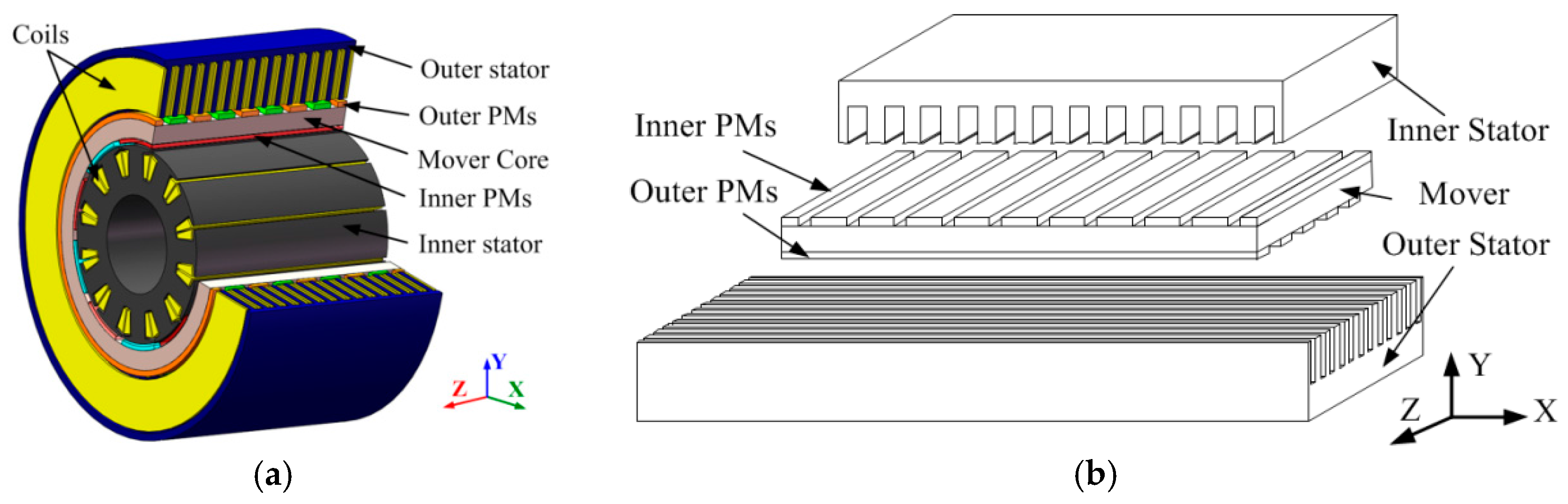
The DSLRPMM consists of two stators and a hollow mover, as shown in Figure 1a. The outer stator adopts a structure of open slots equipped with toroidal coils, while the internal one is a standard isotropic 3-phase stator with semi-closed slots. The windings of the inner and outer stator are all concentrated windings. PMs are affixed on the outer and inner surfaces of the ferromagnetic sleeve core. The ring shaped outer PMs are alternately arranged in the axial direction. The sector shaped inner PMs are putted in the circumferential direction alternately. Obviously, the outer stator and the outer PMs compose the linear motion unit, and the inner stator and inner PMs compose the rotary motion unit.
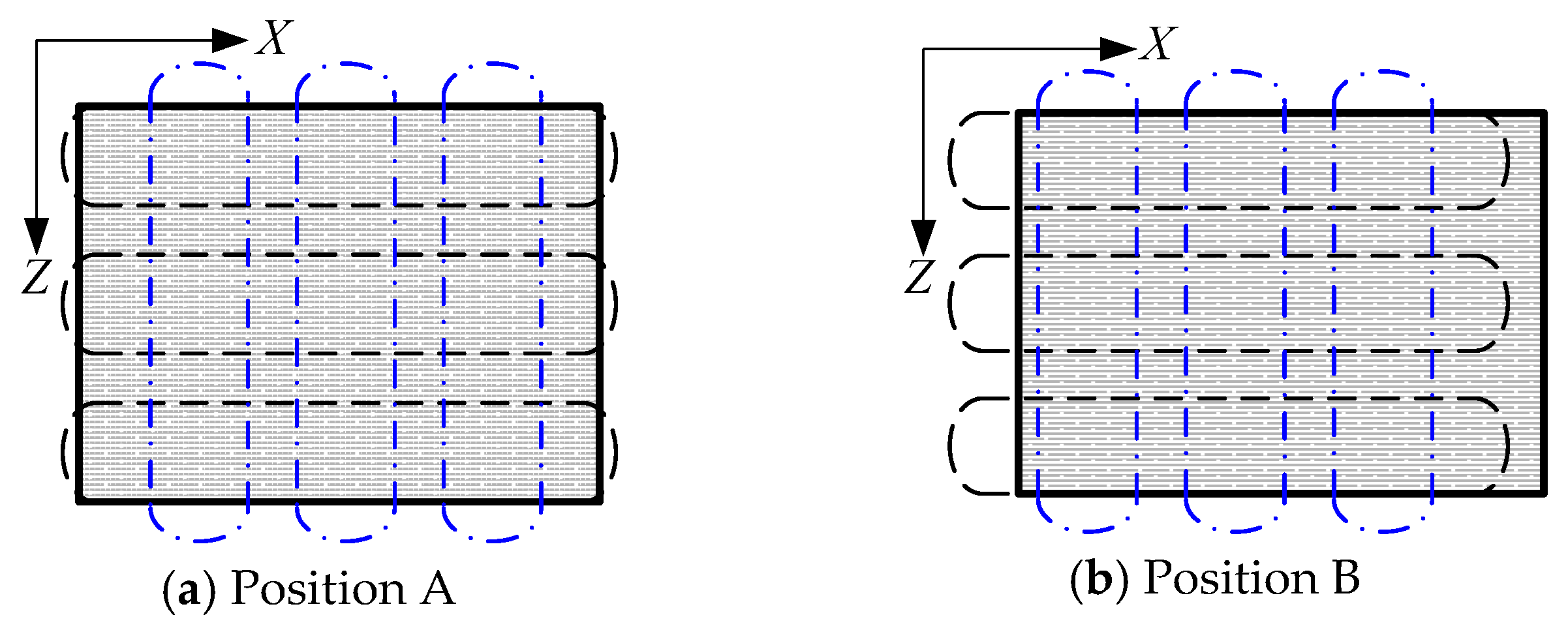
For analyzing the operating principles and establishing the EMCM, the motor shown in Figure 1a is cut along the axial direction and flattened as shown in Figure 1b. Therefore, the linear and rotary movements are converted to the motions of z direction and x direction, respectively. Figure 2 shows the positional relationship between the mover and stator windings in the different operating conditions. The horizontal and vertical arranged dashed boxes represent the windings of the linear motion unit and rotary motion unit, respectively. The dot filled square box denotes the mover. Therefore, three kinds of movement can be expressed as follows:
- (1)
- When the windings of the rotary motion unit are excited by three phase AC currents, the inner armature and PMs will produce the rotating magnetic field, and the mover will move along the x direction (such as from Figure 2a to Figure 2b or Figure 2c to Figure 2d). At the same time the outer PM remains relatively static. Therefore, the rotary motion unit is a standard PMSM.
- (2)
- When the windings of the linear unit are excited by three phase AC currents, the outer armature and PMs will produce the traveling magnetic field, and the mover will move along the z direction (such as from Figure 2a to Figure 2c or Figure 2b to Figure 2d). In this case the linear motion unit is a normal PMLSM.
- (3)
- When the windings of the rotary and linear unit are all excited by three phase AC currents, the rotating and traveling magnetic field will be established in the two air-gaps synchronously. The mover will move along a slant (such as from Figure 2a to Figure 2d or Figure 2b to Figure 2c), which can be called the helical motion.
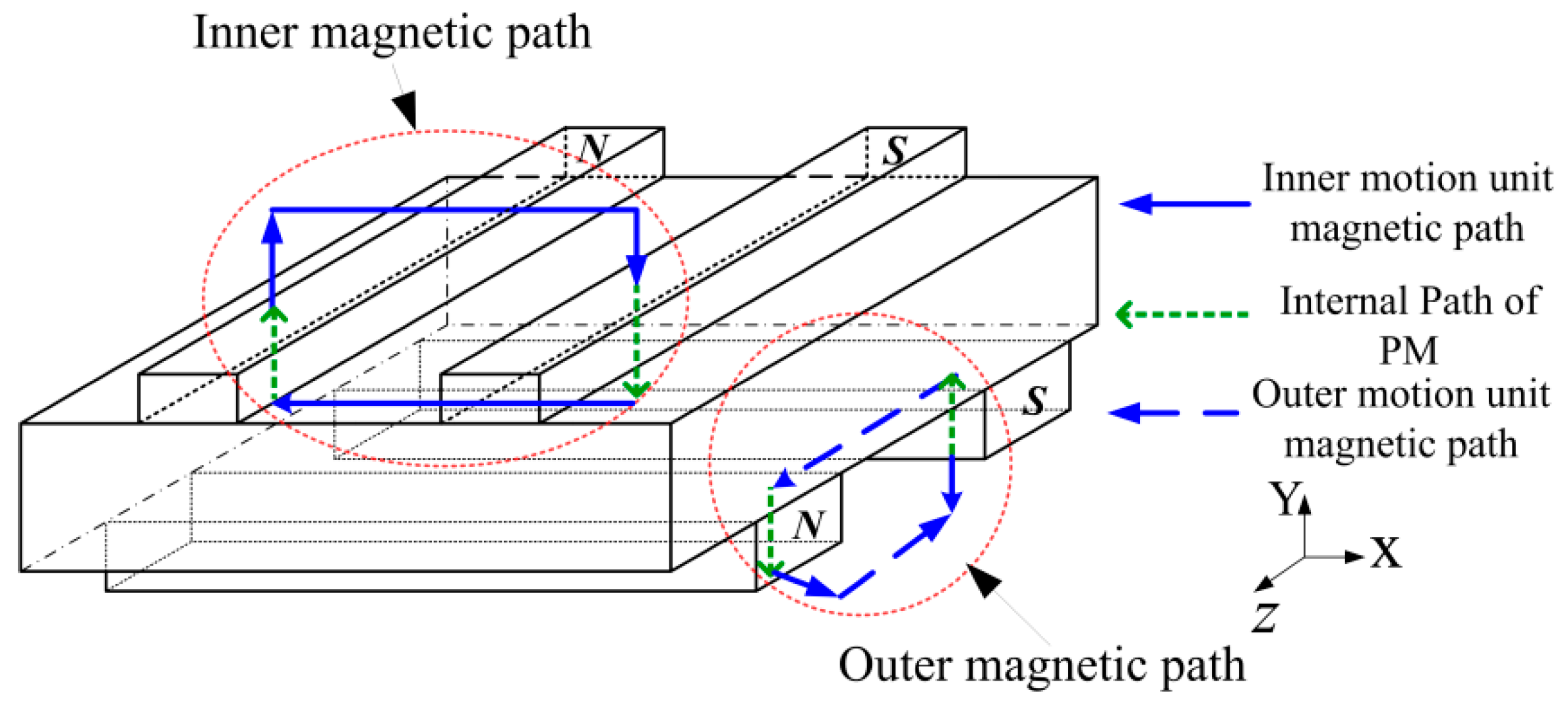
Based on the operating principles, it can be observed that the flux path of the inner and outer motion part is in the x and z direction respectively, and they are independent and orthogonal of each other in the space, as shown in Figure 3.
3. Magnetic Field Calculation and Performances Prediction in Open Circuit
The Maxwell’s equations and Schwarz-Christoffel transformation as the same approach in [24,25] is used to calculate the flux distribution of the two motion unit. Moreover, to take the orthogonally magnetic field coupling effect into account, the equivalent magnetic circuit model is adopted. The following assumptions are made during the calculations in order to reduce the complexity of the computations.
- (1)
- The magnetic material has a uniform magnetization and the relative recoil permeability μr is constant and has a value close to unity such as in NdFeB materials.
- (2)
- For the computation of armature reaction field, the magnet regions are regarded as free space.
- (3)
- Magnetic saturation is absent and the rotor iron cores have infinite magnetic permeability.
- (4)
- Eddy current effects are neglected, which avoids the need for the complex eddy current field formulation.
3.1. Model of the PMs
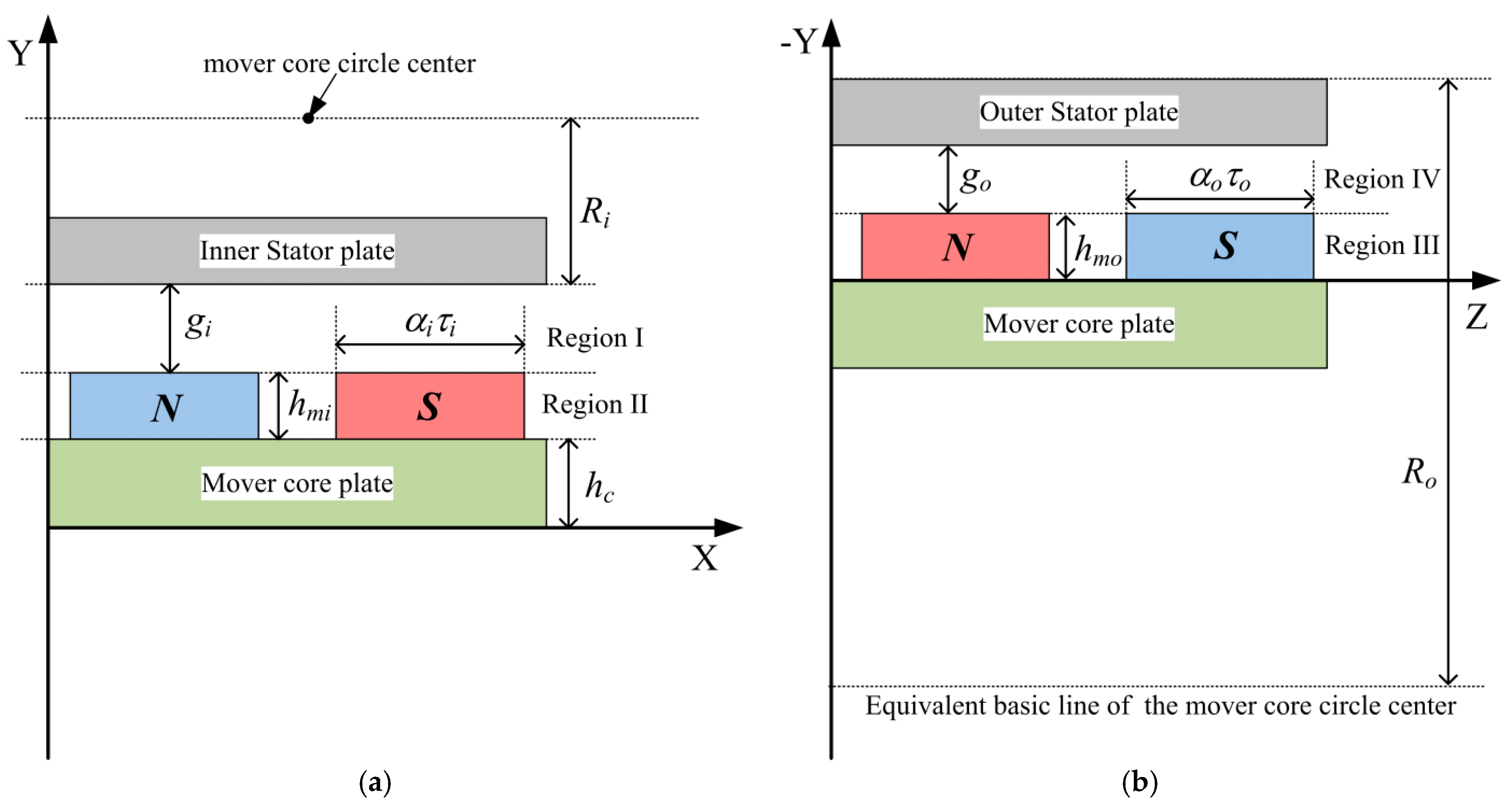
Based on the equivalent planar model, the field of the two motion unit is calculated using Maxwell’s equations by stretching the machine into 2-D model in two planes (the XY plane and ZY plane), respectively. The model of the two motion unit in Cartesian coordinate system is shown in Figure 4. The magnetic induction in the PM is expressed by:
where μrec = μ0μr is the recoil permeability, μ0 = 1 Gs/Oe is the permeability of air.
The magnetization vectors of the inner and outer PMs are all assumed to be along the Y direction and may be described by a Fourier series containing only cosine terms:
where τi and τo are the pole pitch of the rotary and linear motion unit, respectively, Mrn and Mln are respectively expressed as:
The Laplace’s equation as shown in Equation (4) which is valid in both the air space and the PMs is used.
The magnetic field strength related to φ is:
By applying the following boundary conditions to Equation (4):
The flux densities of the x axis, y axis, and z axis in region I, II, III, and IV are solved. For the region I and IV (the inner and outer air space):
and for the region II and III (the inner PMs and outer PMs):
where:
3.2. Model of Armature Reaction Current
Considering the armature winding current effect, the Laplace’s equation is solved again, and the fractional slot windings of the linear and rotary motion unit are assumed as thin wires. The current densities of the two motion units (Ji and Jo) can be obtained by multiplying the value of the current sheet caused by the distribution of the slots in the stator in per unit of each phase, and dividing by the thickness of slot opening (tsoi and tsoo) as follows:
where JAi, JBi, and JCi are the current sheets in per unit of each phase of the rotary motion unit, JAo, JBo, and JCo are the current sheets in per unit of each phase of the linear motion unit. Moreover, in order to obtain the spatial distribution of the currents, the current densities of the two motion unit are, respectively, derived as the following form:
where Ain, Aon, Bin, and Bon are the coefficients obtained from Fourier series, Pi and Po are the number of pole pairs of the rotary and linear motion unit, respectively.
The Laplace’s equation is used in the armature reaction magnetic field calculation, and the solution can be obtained by applying it for the geometries shown in Figure 5. In addition, the following boundary conditions are must applied:
where hi and ho are the positions of a typical armature winding current sheet of rotary and linear motion unit respectively, as shown in Figure 5.
The calculation results of the flux densities in region VI and VIII will be:
where:
3.3. Effect of Stator Slotting
Considering the effects of the stator slotting, the conformal mapping technique is used to transform the geometric shape in Z-plane into a slot-less air gap in T-plane, as shown in Figure 6. As amply illustrated in [26], the effect of stator slotting can be included by defining a vector potential (λ) in each of the stator slots and by linking them to the solution in the air gap region. The components of flux density can be deduced:
where λi and λo can be respectively expressed as:
where λix and λiy are the x axis and y axis components of the complex relative inner air gap permeance in the original Z-plane. λoz and λoy are the z axis and y axis components of the complex relative outer air gap permeance in the original Z-plane.
It should be noticed that the DSLRPMM in the equivalent plane model can be regarded as planar linear permanent magnet machines presented by the Z-plane. Hence, the conformal mapping only transforms the Z-plane to the W-plane by using the Schwarz-Christoffel transformation as the form [27]:
where A is unknown complex constants, n is the number of polygon corners with interior angle αn, ak and bk are the points in the canonical domain (in the W-plane) corresponding to the polygon corners.
The second transformation is to transform the W-plane into the T-plane using the following equation:
where Δx is the slot pitch of the stator (τso and τsi as shown in Figure 6), Δy is the length between the stator core and the mover core.
Based on the conformal transformation, the magnetic flux density at slotted air gap field could be calculated by Equation (18). Afterwards, to obtain the resultant field, the value of the resultant Y-component of PM and armature reaction fields in Equations (9) and (15) should be superimposed. In addition, the X-components of both fields in Equations (10) and (16) should be superimposed as well. The resultant field should be multiplied by the permeance function to obtain the resultant field after considering the slotting effect.
3.4. Effect of the Orthogonal Magnetic Field Coupling
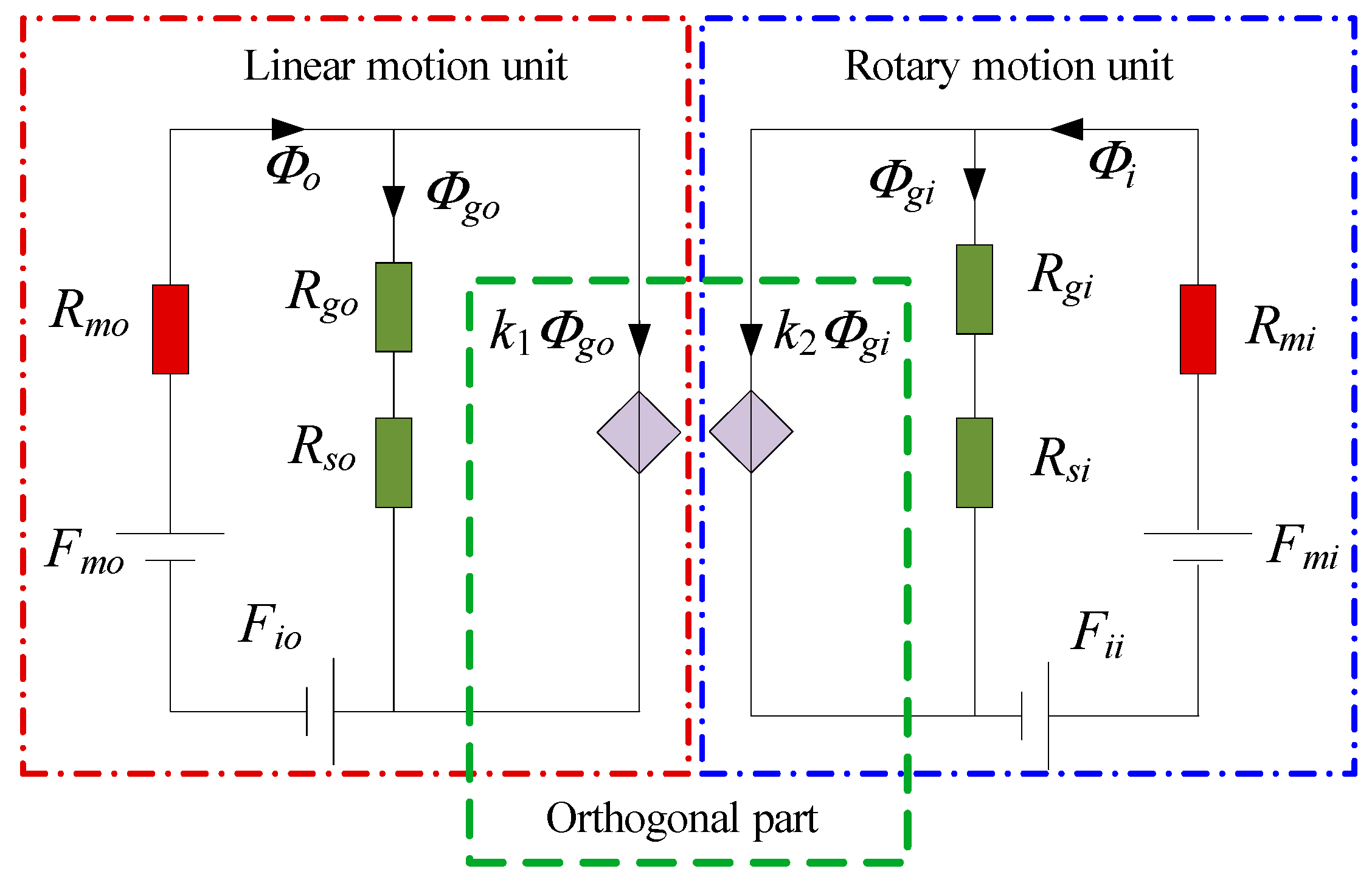
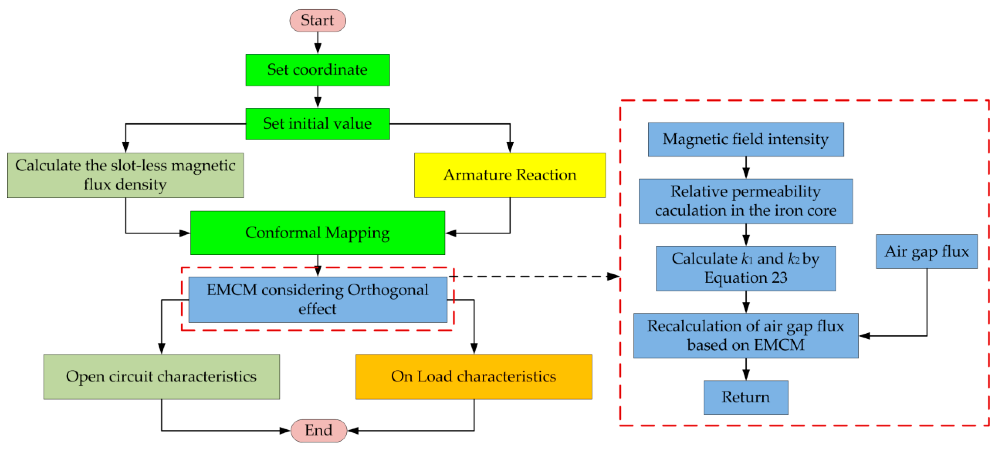
Due to the presence of the orthogonal magnetic fields in the mover core, it is necessary to consider the coupling effect of the two motion unit. In this paper, the equivalent magnetic circuit composite with the Maxwell’s equations is proposed to analyze the effect of the orthogonal magnetic field as shown in Figure 7. In the EMCM, the influences of the orthogonal magnetic field on the two motion unit are equivalent to two controlled sources. The PM fluxes (Φo and Φi) and airgap fluxes (Φgo and Φgi) are calculated using the Maxwell’s equation. k1 and k2 are the coefficient of the orthogonal magnetic field and jointly decided by the inner and outer airgap flux density.
At the different motion condition (linear motion, rotary motion, and helical motion), the value of the coupling coefficients (k1 and k2) are different. The orthogonal magnetic field in the mover core causes the variety of the core relative permeability. Thus, the saturation degree of the mover core is the main factor of the coupling effect. According to the parallel quadrilateral, the vector magnetic field in the mover core is composed of the vector magnetic fields of the inner and outer motion unit. The coupling coefficient of the two motion unit can be given by:
where μs is the resultant relative permeability which is defined by the magnetic field intensity Hc, μrr and μrl are the iron core relative permeability determined by the airgap magnetic field intensity of the rotary motion unit Hi and linear motion unit Ho respectively. The relation between the magnetic field intensity and relative permeability is shown in Figure 8. It should be notice that the values of k1 and k2 are calculated in real-time on the basis of the calculated air gap flux.
3.5. Performances Prediction
3.5.1. Open-Circuit Conditions
In open-circuit condition, the main performances of the DSLRPMM include the cogging torque, detent force, and back EMF. The cogging torque of the rotary motion unit is calculated by the changing rate of the total air gap co-energy including the region of PMs [28]:
The detent force of the linear motion unit consists of the cogging force and end force. The cogging force Fs is a periodic function of the slot pitch, and the end force Fe is a periodic function of the pole pitch. The detent force can be expressed as
where:
where Fsn and Fcn are the magnitudes of the nth harmonic component. Lo is the length of the out stator.
The back EMF waveform of the DSLRPMM can be calculated from the no-load flux density distribution (By) with the knowledge of the armature winding distribution. The voltage induced in a phase can be calculated as:
where Ni and No are the effective number of turns per phase of rotary and linear motion unit respectively, Bi(θ) and Bo(θ) are the flux density at a given electrical spatial position of the rotary and linear motion unit respectively, Ravei and Raveo are the average radial of the stator of the rotary and linear motion unit, respectively, Li is the equivalent length of the inner air gap.
3.5.2. On-Load Conditions
The electromagnetic torque and force could be calculated using Maxwell stress tensor method near the center of the air gap. The torque and force can be expressed as:
where Bari and Bati are the radial and tangential air gap flux densities of the rotary motion unit with armature reaction, respectively. Baro and Bazo are the radial and tangential air gap flux densities of the linear motion unit with armature reaction, respectively.
3.6. Process of the Calculation
Based on the analysis above, the analytical model of the DSLRPMM can be established by using the software of Matrix Laboratory (MATLAB, The MathWorks, Natick, MA, USA). The open circuit characteristics, including the cogging torque, cogging force, end force, detent force, and back-EMFs, are calculated, and the on-load characteristics are also analyzed. Figure 9 shows the calculation processes.
4. Comparison of Predictions with Finite Element Calculation
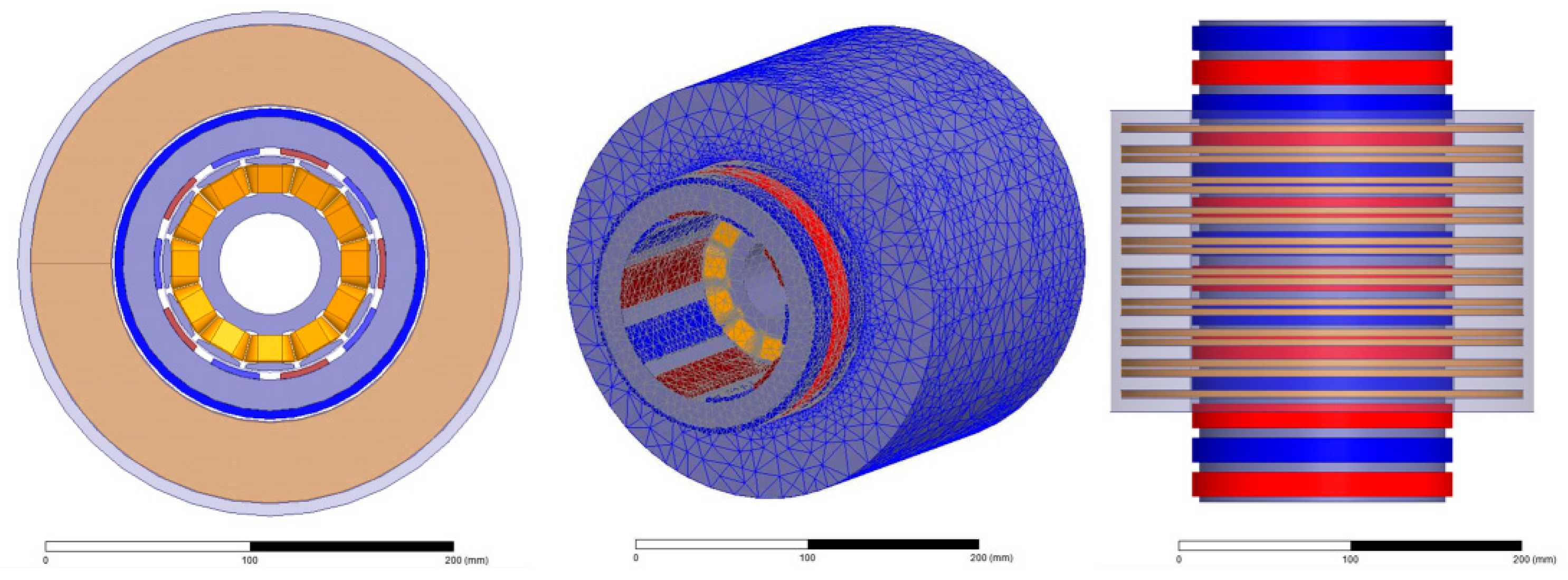
The DSLRPMM used for investigation was designed and the major design parameters of the motor are listed in Table 1. The model of the motor using 3D finite element method (FEM) is established, as shown in Figure 10. The rotary motion unit is a structure of 12-slots/10-poles, and the linear motion unit is a structure of 9-slots/8-poles.
The calculated radial flux density waveforms compared with the FEM results are shown in Figure 11. It is clear that the analytical calculated radial airgap flux densities considering the orthogonal effect (OE) are agreed well with that obtained by the 3D FE analysis. Figure 12 shows the tangential flux density waveforms, the analytical results also coincide with the 3D FEM analysis. The calculated tangential flux densities are consistent with the results of the FE analysis very well both of the rotary and linear motion unit. The analytical flux densities without considering the orthogonal effect are all bigger than that of considering the OE in the rotary and linear motion unit. It can also be noted that the model without considering the orthogonal effect get 2.5% and 8.8% error rates when calculate the flux density of the rotary and linear motion unit respectively.
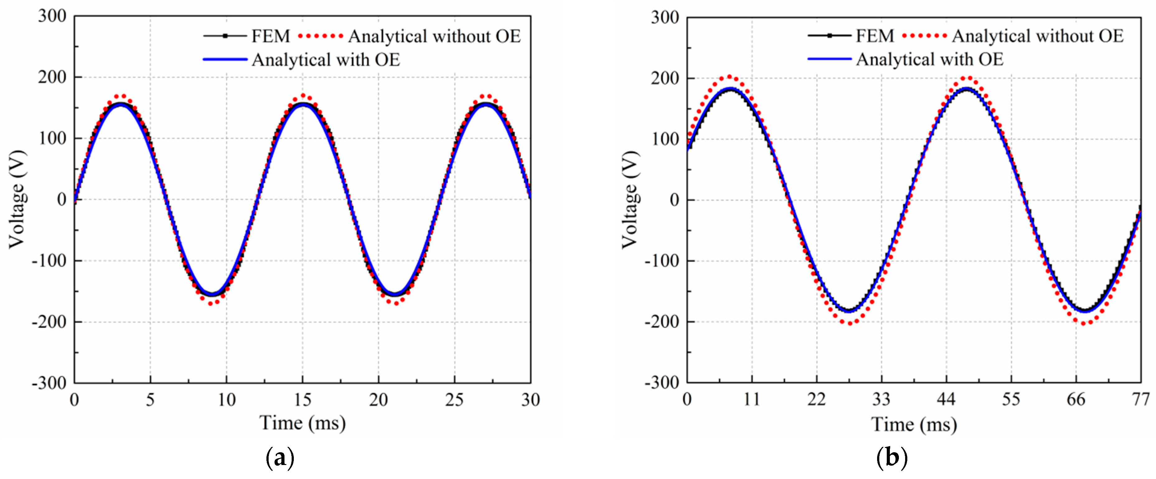
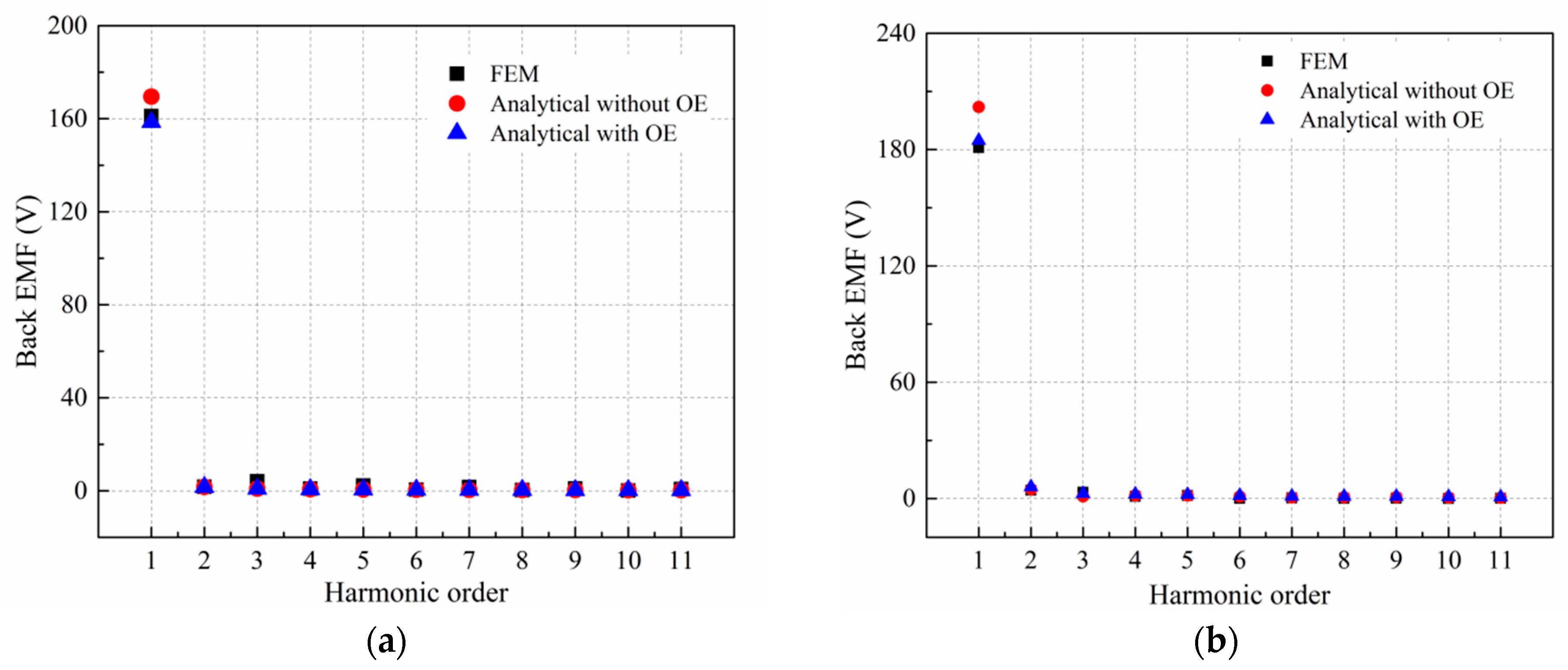
The back EMFs of the rotary and linear motion unit are shown in Figure 13, and the speeds of the rotary and linear motion are 1000 r/min and 1 m/s, respectively. The maximum calculated back EMF values of the rotary motion unit are, respectively, 158 V and 165 V with and without OE, and that of the linear motion unit are 185 V and 202 V, respectively. As shown in Figure 14, the fundamental values of the back EMF of the analytical model without OE are all larger than that of the results obtained by FEM and the calculated model with OE. The fundamental values of the rotary and linear motion unit calculated by the model with OE are essentially in agreement with that of FEA. In addition, the 3th harmonic obtained by the FEM is bigger than that of the calculated results. This is caused by the local saturation of the core which is not considered in the analytical model.
The cogging torque is shown in Figure 15a. The analytical computation result shows good consistency with the FE analysis and the peak to peak value is 244 mN·m. The calculated peak to peak value of the cogging torque without considering orthogonal effect is 260 mN·m. Figure 15b shows the detent force of the motor. Due the detent force of the linear motion consists of cogging force and end force, the two parts are calculated respectively in the analytical model, and the results are shown in Figure 15c,d, respectively. The peak to peak value of the detent force is 90 N, and the maximum value of the cogging force and end force is 105 N and 130 N respectively. It should be noted that the cogging force and torque are affected by the orthogonal magnetic field evidently, but it has no effect on the end force due to the weakness of the OE phenomenon at the end of the outer stator.
5. Experimental Results
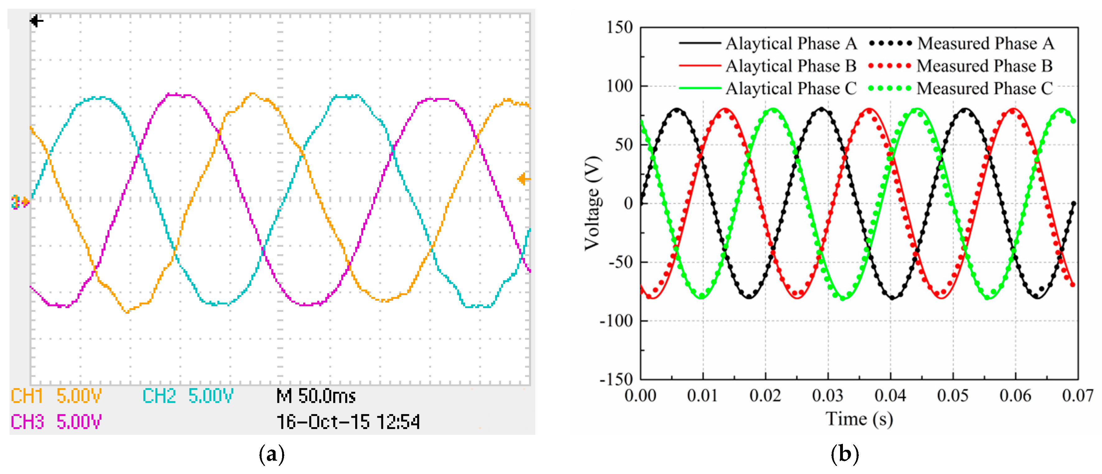
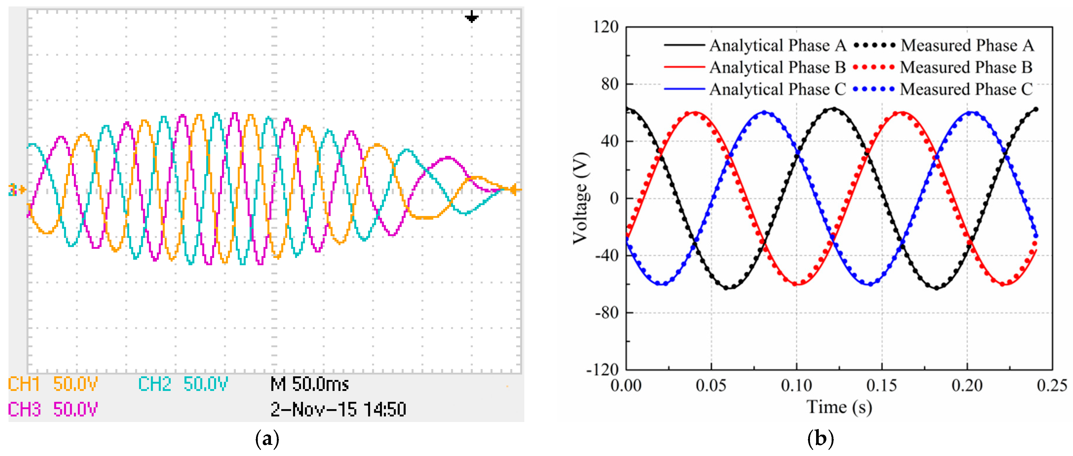
The constructed prototype with the parameters listed in Table 1 and its components are shown in Figure 16a. The experimental setup, including prototype, rotary load, linear load, and controller, is shown in Figure 16b. A weight as linear load is connected with the mover by the wire rope and pulley, and a motor as rotary load is coupled with the mover via the cone belt. The frequency converter is used to control the DSLRPMM. The back EMF of the two motion units are measured and compared with that predicted by the analytical model. The back EMF waveforms of the rotary motion unit are given in Figure 17. Figure 18 shows the back EMFs of the linear motion unit. As can be see, the measured and predicted back EMF are sinusoidal and in good agreement.
The comparison of the back EMF and time for analytical calculation and FEM is shown in Table 2. It can be observed that there is a slight error between the analytical and FEM which is mainly caused by the accuracy of the EMCM, and the error between the measured and simulated is caused by the assembling accuracy. Considering the CPU computing time, the analytical model just requires 9 min to finish the calculation of the motor in open circuit. 3D FEM, on the other hand, requires almost 24 h with 300 million computational nodes for each step. Although the analytical prediction shows a petty error compared to the experimental result, it is still acceptable and thus, can be regarded as a meaningful approach which could save time and achieve a satisfying result. In addition, the analytical model could also be used for further optimization, design parameter and performance prediction, etc.
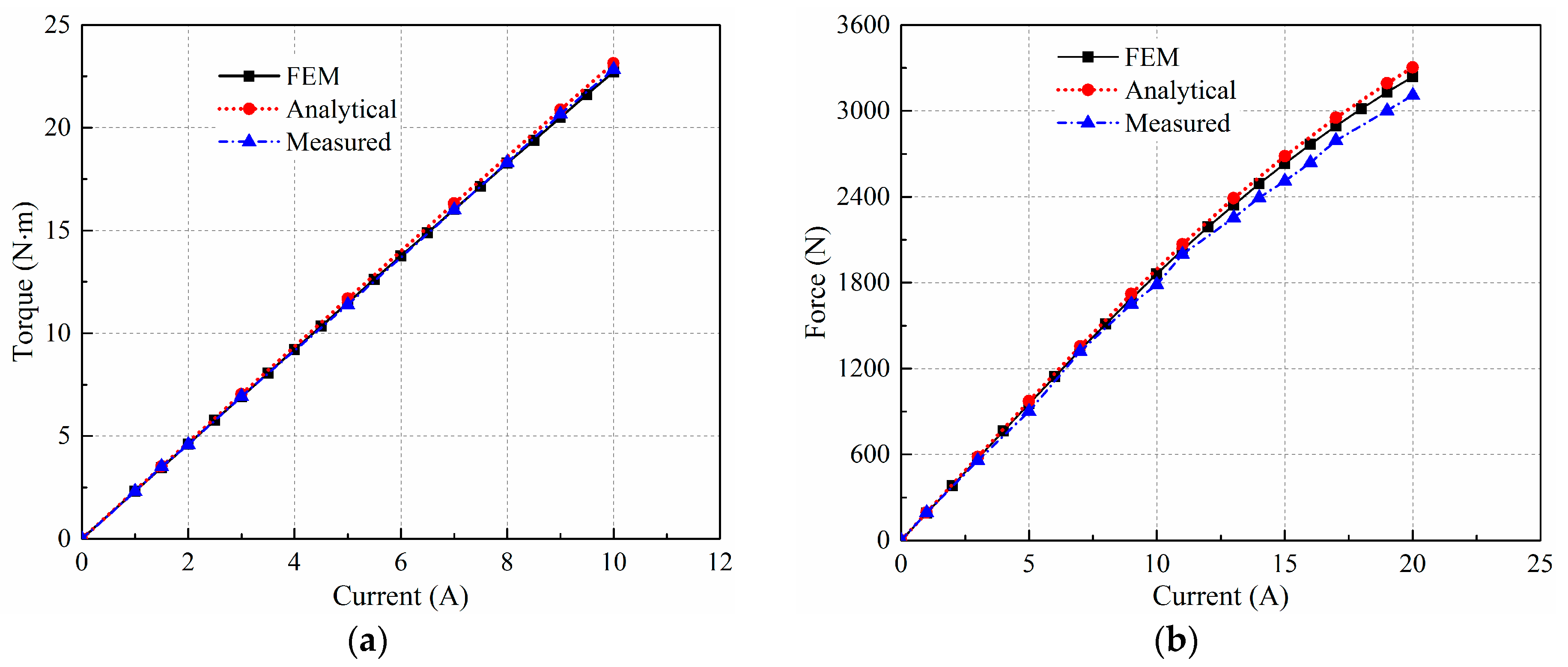
Figure 19 shows the torque and force characteristics under the different loading conditions. It is clearly that the computed results consistent with that obtained both by the 3D FE analysis and measurements, and the torque-current and force-current characteristics are almost linear. At the rated output power, the measured currents of the rotary and linear motion unit are 4.2 A and 11 A, respectively, and they meet the design requirements. It should be noted that due to the friction effects, the measured force of the linear motion unit is smaller than that obtained by the analytical analysis under the heavy load conditions.
6. Conclusions
A DSLRPMM with two stators and a hollow mover is presented and broadened as a plane surface-mounted permanent magnet machine for analytical analysis in this paper. Due to the intrinsic 3D magnetic field distribution nature of the DSLRPMM, a quasi-3D method based upon the combined solution of Maxwell’s solution and EMCM is used to analytical predict the performance of the DSLRPMM, and the orthogonal magnetic field effect is considered. The DSLRPMM with 12/10-pole and 9/8-pole is investigated based on the proposed analytical method. The magnetic field, back EMF, cogging torque, detent force, and output torque and force of the DSLRPMM are calculated with great accuracy compared to the 3D FE analysis, and the analytical model with and without considering the OE is also investigated and compared. Moreover, under time comparison, the analytical model was up to 160 times faster compared with 3D FEM. At the end, the experimental verification has been carried out based on a prototype of the DSLRPMM, and the results are consistent with the simulation results obtained by the proposed method. In conclusion, the analytical model has proven to act very well with the DSLRPMM geometries and loading conditions in a very effective time and can be used for the analysis of the orthogonal magnetic field conditions.
Acknowledgments
This work was supported by the National Natural Science Foundation of China under Grant 51307022, by the Natural Science Foundation of Jiangsu Province, China, under Grant BK20130611, by the China Postdoctoral Science Foundation under Grant 2014M550260, by the China Postdoctoral Foundation Special Project under Grant 2015T80479.
Author Contributions
Each of the authors contributes on performing experiments and writing articles. Lei Xu is the main authors of this manuscript and this work was conducted under advisement of Mingyao Lin. Xinghe Fu, Kai Liu and Baocheng Guo helped to finish the experiments. All authors revised and approved the publication.
Conflicts of Interest
The authors declare no conflict of interest.
References
- Mendrela, E.A.; Gierczak, E.C. Double-winding rotary-linear induction motor. IEEE Trans. Energy Convers. 1987, EC-2, 47–54. [Google Scholar] [CrossRef]
- Jeon, W.J.; Tanabiki, M.; Onuki, T.; Yoo, J.Y. Rotary-linear induction motor composed of four primaries with independently energized ring-windings. In Proceedings of the IEEE Industry Application Society Annual Meeting, New Orleans, LA, USA, 5–9 October 1997; pp. 365–372. [Google Scholar]
- Jin, P.; Fang, S.H.; Lin, H.Y.; Wang, X.B.; Zhou, S.G. A novel linear and rotary halbach permanent magnet actuator with two degrees-of-freedom. J. Appl. Phys. 2012, 111. [Google Scholar] [CrossRef]
- Pan, J.F.; Zou, Y.; Cheung, N.C. Investigation of a rotary-linear switched reluctance motor. In Proceedings of the 2010 XIX International Conference on Electrical Machines(ICEM), Rome, Italy, 6–8 September 2010; pp. 1–4. [Google Scholar]
- Pan, J.F.; Zou, Y.; Cheung, N.C. Performance analysis and decoupling control of an integrated rotary linear machine with coupled magnetic paths. IEEE Trans. Magn. 2014, 50, 761–764. [Google Scholar] [CrossRef]
- Si, J.K.; Feng, H.C.; Ai, L.W.; Hu, Y.H.; Cao, W.P. Design and analysis of a 2-DOF split-stator induction motor. IEEE Trans. Energy Convers. 2015, 30, 1200–1208. [Google Scholar] [CrossRef]
- Jang, S.M.; Lee, S.H.; Cho, H.W.; Cho, S.K. Design and analysis of helical motion permanent magnet motor with cylindrical halbach array. IEEE Trans. Magn. 2003, 39, 3007–3009. [Google Scholar] [CrossRef]
- Bolognesi, P.; Taponecco, L. A novel 2-freedom-degree brushless motor. In Proceedings of the 2002 IEEE International Symposium on Industrial Electronics (ISIE), L’Aquila, Italy, 8–11 July 2002; pp. 863–868. [Google Scholar]
- Krebs, G.; Tounzi, A.; Pauwels, B.; Piriou, F. Modeling of a linear and rotary permanent magnet actuator. IEEE Trans. Magn. 2008, 44, 4357–4360. [Google Scholar] [CrossRef]
- Krebs, G.; Tounzi, A.; Pauwels, B.; Willemot, D.; Piriou, M.F. Design of a permanent magnet actuator for linear and rotary movements. Eur. Phys. J. Appl. Phys. 2008, 44, 77–85. [Google Scholar] [CrossRef]
- Jin, P.; Lin, H.Y.; Fang, S.H.; Yuan, Y.; Guo, Y.J.; Jia, Z. 3D Analytical linear force and rotary torque analysis of linear and rotary permanent magnet actuator. IEEE Trans. Magn. 2013, 49, 3989–3992. [Google Scholar] [CrossRef]
- Chen, L.; Hofmann, W. Design of one rotary-linear permanent magnet motor with two independently energized three phase windings. In Proceedings of the 7th IEEE International Conference on Power Electronics and Drive Systems (PEDS), Bangkok, Thailand, 26–30 November 2007; pp. 1372–1376. [Google Scholar]
- Meessen, K.J.; Paulides, J.J.H.; Lomonova, E.A. Analysis of a novel magnetization pattern for 2-DOF rotary-linear actuators. IEEE Trans. Magn. 2012, 48, 3867–3870. [Google Scholar] [CrossRef]
- Xu, L.; Lin, M.Y.; Fu, X.H.; Li, N. Analysis of a double stator linear rotary permanent magnet motor with orthogonally arrayed permanent magnets. IEEE Trans. Magn. 2016, 52. [Google Scholar] [CrossRef]
- Zheng, P.; Wu, Q.; Zhao, J.; Tong, C.D.; Bai, J.G.; Zhao, Q.B. Performance analysis and simulation of a novel brushless double rotor machine for power-split HEV applications. Energies 2012, 5, 119–137. [Google Scholar] [CrossRef]
- Tong, C.D.; Song, Z.Y.; Bai, J.G.; Liu, J.Q.; Zheng, P. Analytical investigation of the magnetic-field distribution in an axial magnetic-field-modulated brushless double-rotor machine. Energies 2016, 9, 589. [Google Scholar] [CrossRef]
- Huang, Y.K.; Guo, B.C.; Hemeida, A.; Sergeant, P. Analytical modeling of static eccentricities in axial flux permanent-magnet machines with concentrated windings. Energies 2016, 9, 892. [Google Scholar] [CrossRef]
- Bianchi, N. Analytical field computation of a tubular permanent-magnet linear motor. IEEE Trans. Magn. 2000, 36, 3798–3801. [Google Scholar] [CrossRef]
- Li, W.; Chau, K.T. Analytical field calculation for linear tubular magnetic gears using equivalent anisotropic magnetic permeability. Prog. Electromagn. Res. 2012, 127, 155–171. [Google Scholar] [CrossRef]
- Yu, Y.J.; Zhang, W.Y.; Sun, Y.X.; Xu, P.F. Basic characteristics and design of a novel hybrid magnetic bearing for wind turbines. Energies 2016, 9, 905. [Google Scholar] [CrossRef]
- Jin, P.; Fang, S.H.; Lin, H.Y.; Zhu, Z.Q.; Huang, Y.K.; Wang, X.B. Analytical magnetic field analysis and prediction of cogging force and torque of a linear and rotary. IEEE Trans. Magn. 2011, 47, 3004–3007. [Google Scholar] [CrossRef]
- Meessen, K.J.; Paulides, J.J.H.; Lomonova, E.A. Modeling of magnetization patterns for 2-DoF rotary-linear actuators. Int. J. Comput. Math. Electr. Electron. Eng. 2012, 31, 1428–1440. [Google Scholar] [CrossRef]
- Guo, K.K.; Fang, S.H.; Zhang, Y.; Yang, H.; Lin, H.Y.; Ho, S.L.; Feng, N.J. Irreversible demagnetization analysis of permanent magnet materials in a novel flux reversal linear-rotary permanent magnet actuator. IEEE Trans. Magn. 2016, 52. [Google Scholar] [CrossRef]
- O’Connell, T.C.; Krein, P.T. A Schwarz–Christoffel-based analytical method for electric machine field analysis. IEEE Trans. Energy Convers. 2009, 24, 565–577. [Google Scholar] [CrossRef]
- Hemeida, A.; Sergeant, P. Analytical modeling of surface PMSM using a combined solution of Maxwell’s equations and magnetic equivalent circuit. IEEE Trans. Magn. 2014, 50. [Google Scholar] [CrossRef]
- Zarko, D.; Ban, D.; Lipo, T.A. Analytical calculation of magnetic field distribution in the slotted air gap of a surface permanent magnet motor using complex relative air-gap permeance. IEEE Trans. Magn. 2004, 42, 1828–1837. [Google Scholar] [CrossRef]
- Gibbs, W.J. Conformal Transformations in Electrical Engineering; Chapman & Hall: London, UK, 1958; pp. 56–59. [Google Scholar]
- Barakat, G.; El-Meslouhi, T.; Dakyo, B. Analysis of the cogging torque behavior of a two-phase axial flux permanent magnet synchronous machine. IEEE Trans. Magn. 2001, 37, 2803–2805. [Google Scholar] [CrossRef]
Figure 1.
Configuration of the DSLRPMM. (a) 3D cutaway view of the DSLRPMM; and (b) equivalent planar model of the DSLRPMM.
Figure 1.
Configuration of the DSLRPMM. (a) 3D cutaway view of the DSLRPMM; and (b) equivalent planar model of the DSLRPMM.

Figure 2.
Positional relationship between mover and windings in different motion.


Figure 3.
Flux path of the DSLRPMM.

Figure 4.
Model of no-load air-gap flux caused by magnets. (a) Field region of the rotary motion unit in XY plane; and (b) field region of the linear motion unit in ZY plane.
Figure 4.
Model of no-load air-gap flux caused by magnets. (a) Field region of the rotary motion unit in XY plane; and (b) field region of the linear motion unit in ZY plane.

Figure 5.
Current sheet model for armature reaction computation. (a) Field region of the rotary motion unit in XY plane; and (b) field region of the linear motion unit in ZY plane.
Figure 5.
Current sheet model for armature reaction computation. (a) Field region of the rotary motion unit in XY plane; and (b) field region of the linear motion unit in ZY plane.
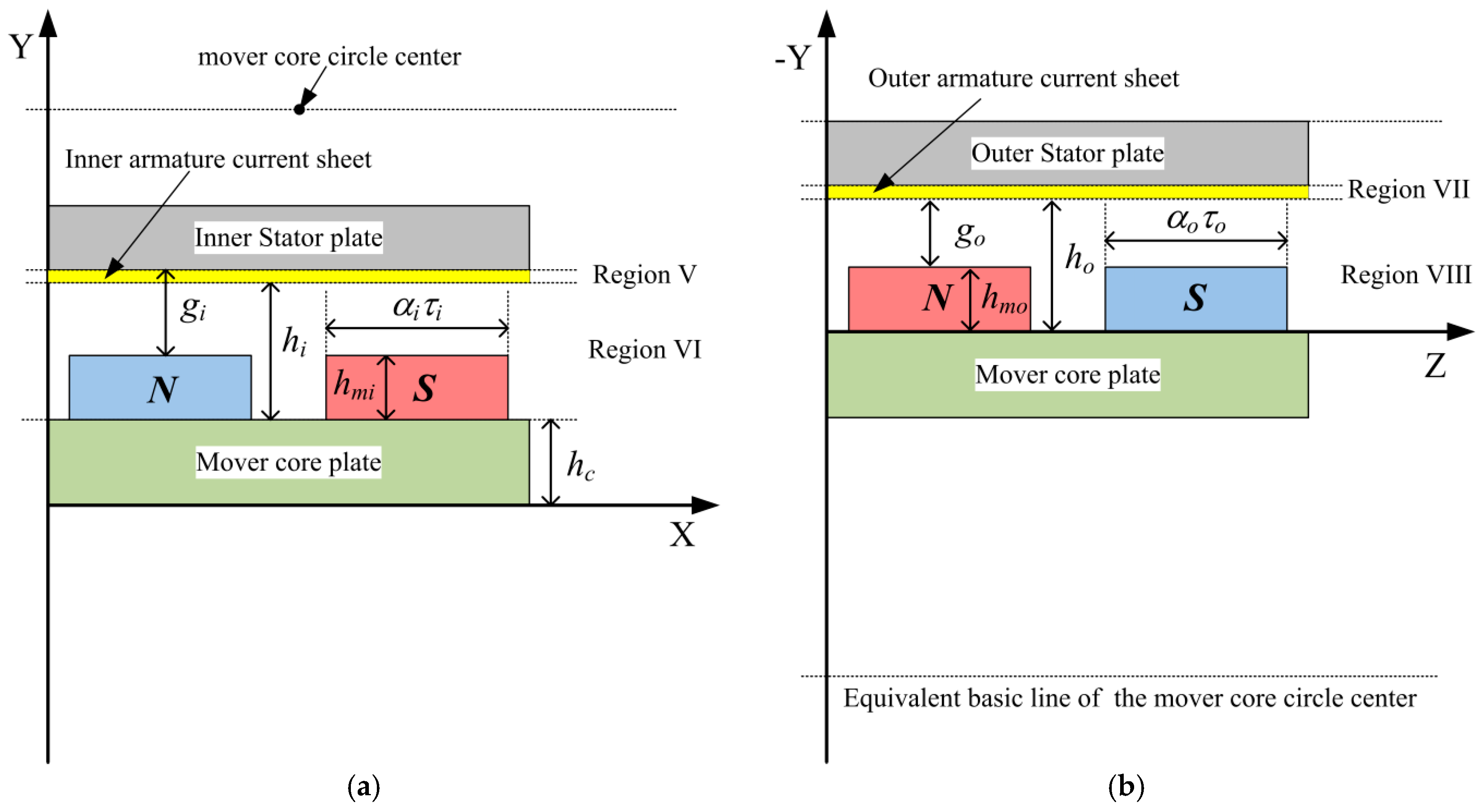
Figure 6.
Slot opening in different planes.
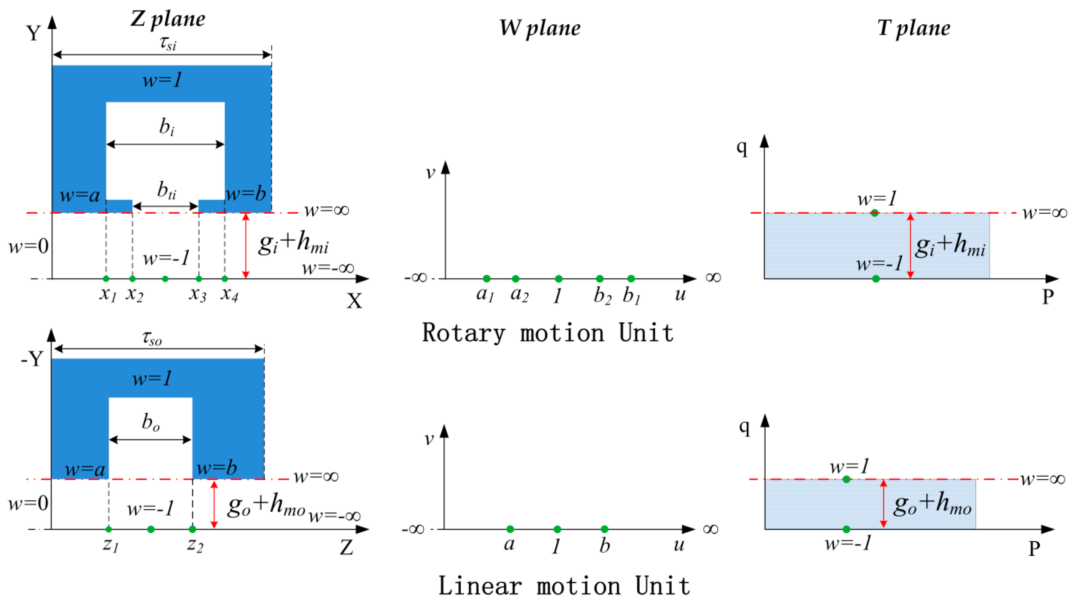
Figure 7.
Equivalent magnetic model of the DSLRPMM with Maxwell’s resultant flux.

Figure 8.
Relation between the magnetic field intensity and relative permeability of the used mover core material.
Figure 8.
Relation between the magnetic field intensity and relative permeability of the used mover core material.
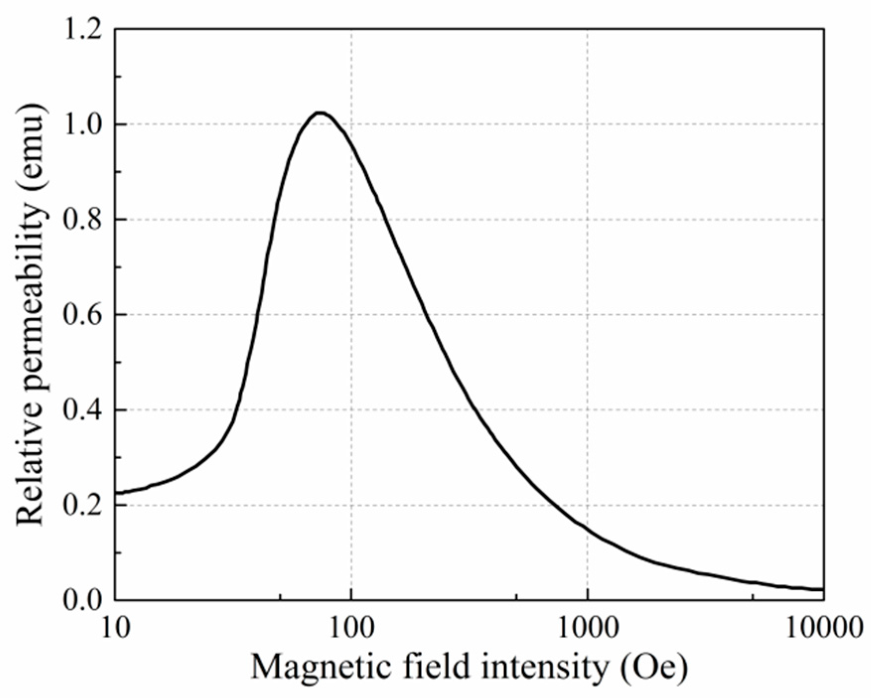
Figure 9.
Calculation process.

Figure 10.
3D FE model and its mesh.

Figure 11.
Radial flux density of the DSLRPMM. (a) Rotary motion unit; and (b) linear motion unit.
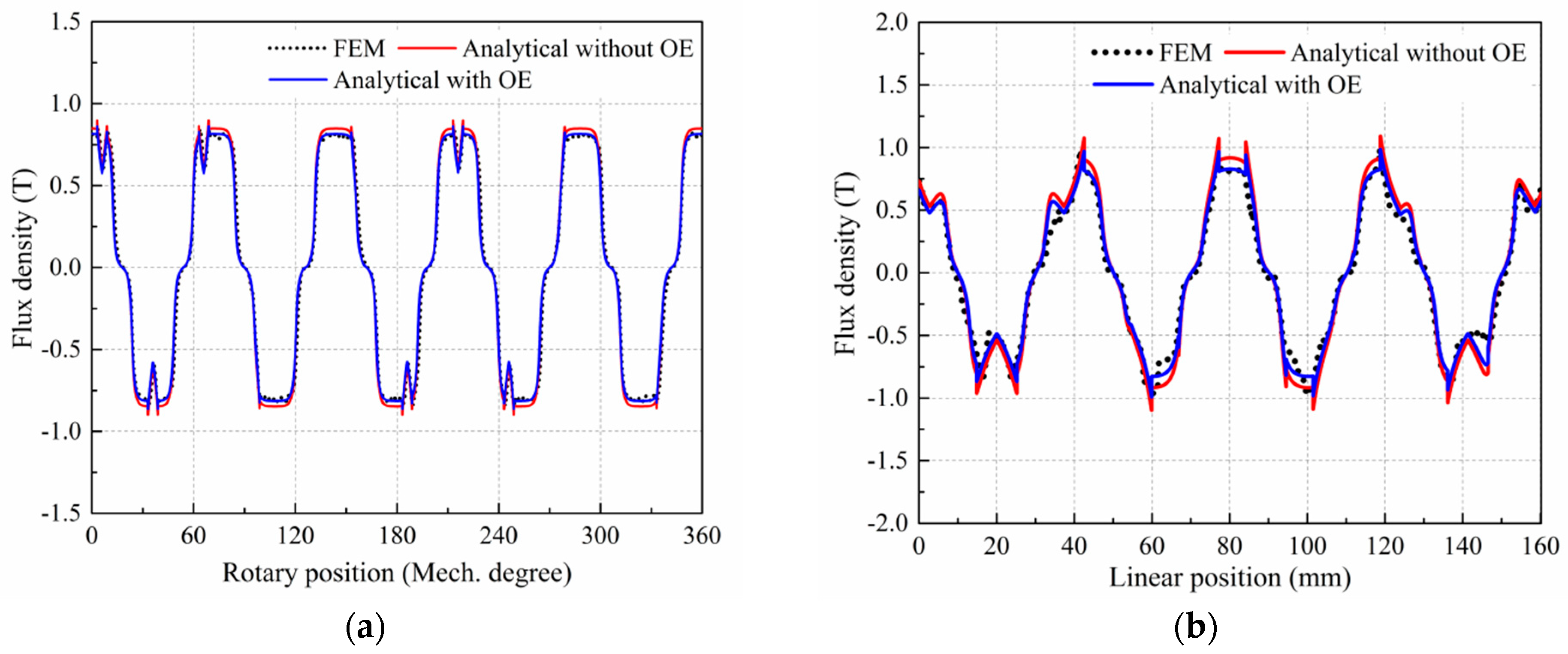
Figure 12.
Tangential flux density of the DSLRPMM. (a) Rotary motion unit; and (b) linear motion unit.
Figure 12.
Tangential flux density of the DSLRPMM. (a) Rotary motion unit; and (b) linear motion unit.
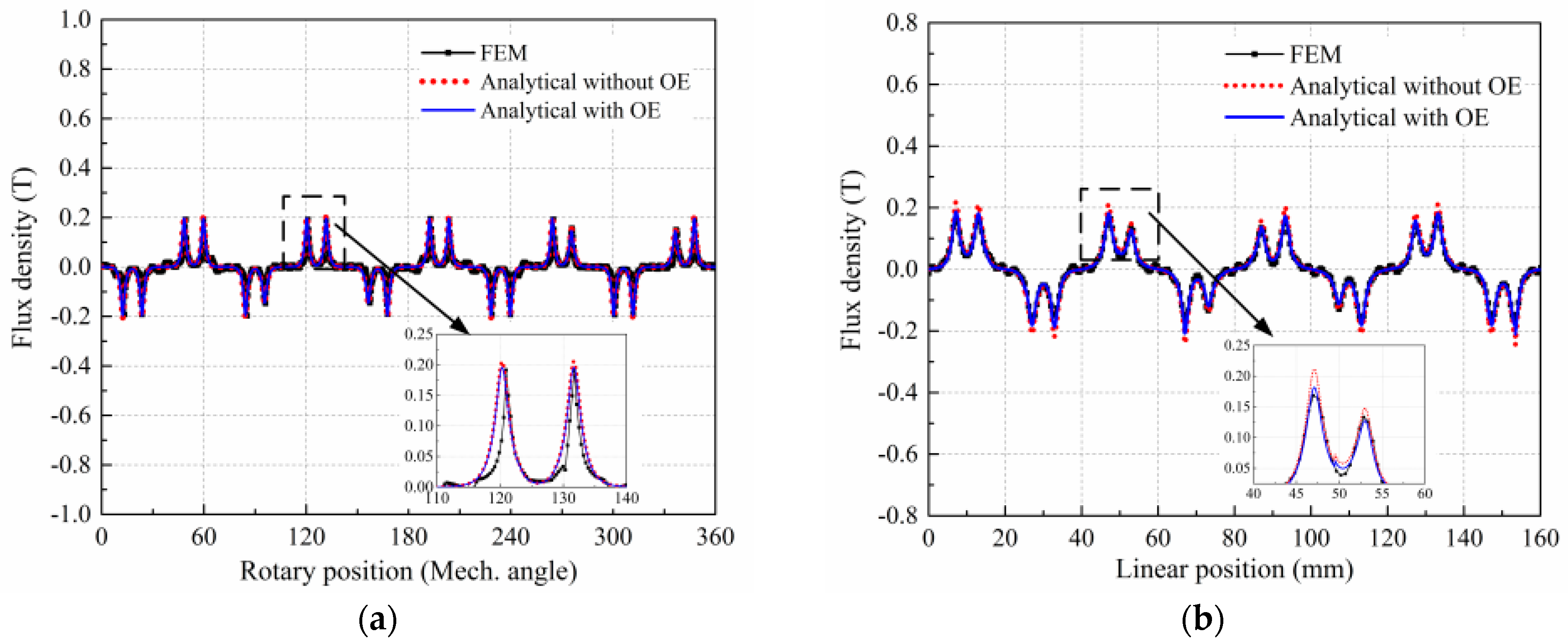
Figure 13.
Back EMF of the DSLRPMM. (a) Rotary motion unit. (b) Linear motion unit.

Figure 14.
Harmonic of back EMFs. (a) Rotary motion unit. (b) Linear motion unit.

Figure 15.
(a) Cogging torque of the rotary motion unit; (b) detent force of the linear motion unit; (c) cogging force of the linear motion unit; and (d) end force of the linear motion unit.
Figure 15.
(a) Cogging torque of the rotary motion unit; (b) detent force of the linear motion unit; (c) cogging force of the linear motion unit; and (d) end force of the linear motion unit.
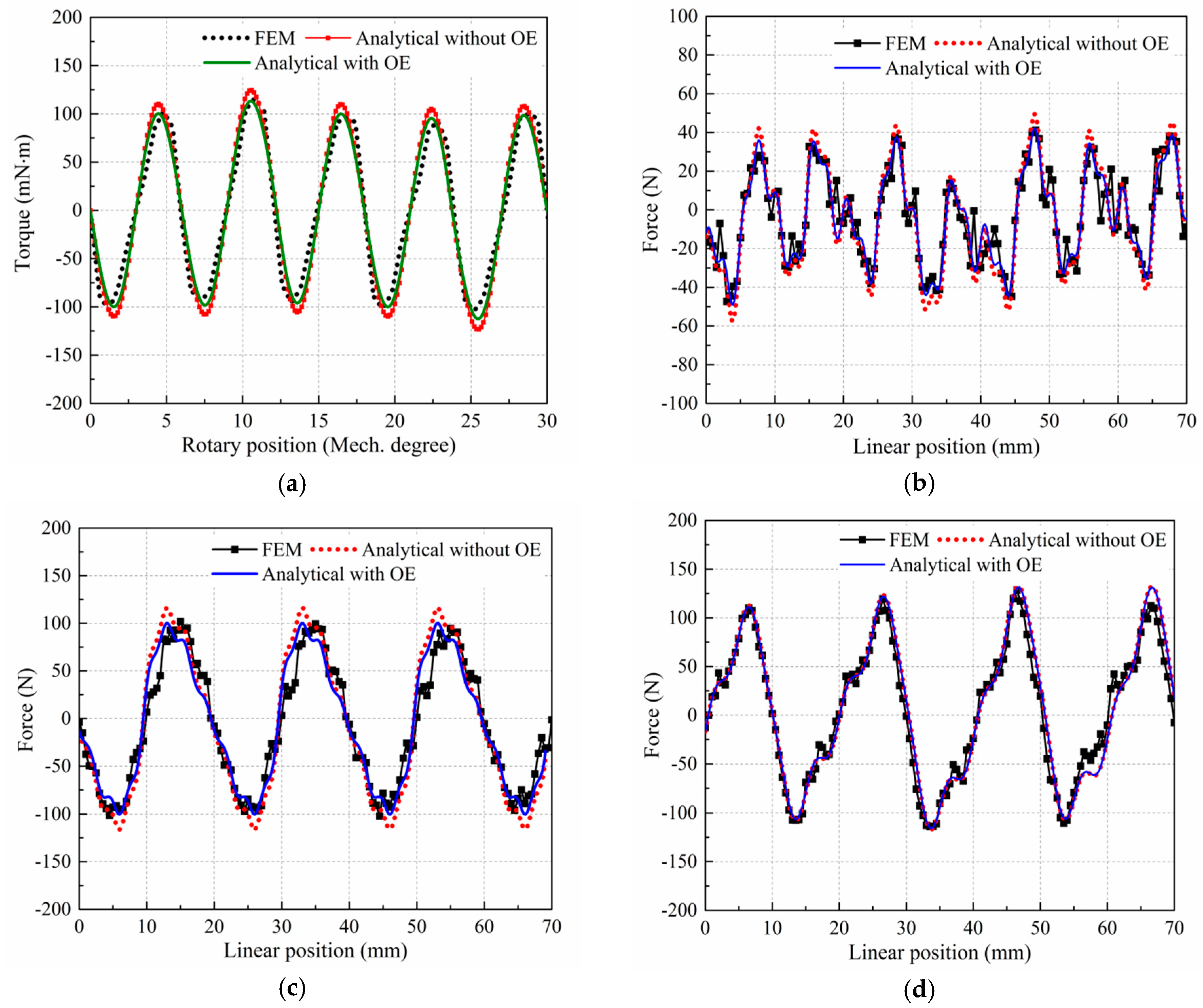
Figure 16.
(a) Prototype and its components; and (b) experimental setup.
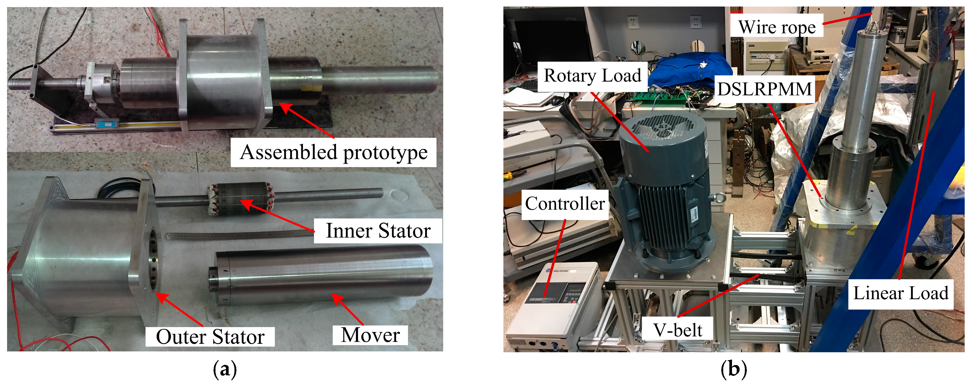
Figure 17.
(a) Measured back EMF of the rotary motion unit at 50 r/min; and (b) comparison of the analytical and measured back EMF of the rotary motion unit at 520 r/min.
Figure 17.
(a) Measured back EMF of the rotary motion unit at 50 r/min; and (b) comparison of the analytical and measured back EMF of the rotary motion unit at 520 r/min.

Figure 18.
(a) Measured back EMF of the linear motion unit at the average speed of 0.68 m/s; and (b) comparison of the analytical and measured back EMF of the linear motion unit at 0.33 m/s.
Figure 18.
(a) Measured back EMF of the linear motion unit at the average speed of 0.68 m/s; and (b) comparison of the analytical and measured back EMF of the linear motion unit at 0.33 m/s.

Figure 19.
(a) Torque characteristics at rated speed; and (b) force characteristics at rated speed.

Table 1.
Parameters of the DSLRPMM.
| Items | Value | Items | Value |
|---|---|---|---|
| Rated rotary motion power | 1 kW | Inside diameter of mover core | 114 mm |
| Rated linear motion power | 1 kW | Outside diameter of mover core | 144 mm |
| Rated rotational speed | 1000 r/min | Outer diameter of outer stator | 247 mm |
| Rated linear speed | 1 m/s | Inner diameter of inner stator | 50 mm |
| Inner PM thickness | 3 mm | Outer air-gap length | 1.5 mm |
| Outer PM thickness | 4 mm | Inner air-gap length | 1.5 mm |
| Axial length of the inner stator | 106 mm | Axial length of the outer stator | 175.4 mm |
Table 2.
Comparison of back EMF with experiment result.
| Item | Analytical Rotary | Analytical Linear | FEM Rotary | FEM Linear | Measured Rotary | Measured Linear |
|---|---|---|---|---|---|---|
| RMS value of back EMF (V) | 60.25 | 46.1 | 60.2 | 46 | 60 | 45.8 |
| Error in voltage | −0.42% | −0.66% | −0.33% | −0.44% | - | - |
| CPU time (h) | 0.15 | 24 | - | - | ||
© 2017 by the authors. Licensee MDPI, Basel, Switzerland. This article is an open access article distributed under the terms and conditions of the Creative Commons Attribution (CC BY) license (http://creativecommons.org/licenses/by/4.0/).
Share and Cite
MDPI and ACS Style
Xu, L.; Lin, M.; Fu, X.; Liu, K.; Guo, B. Analytical Calculation of the Magnetic Field Distribution in a Linear and Rotary Machine with an Orthogonally Arrayed Permanent Magnet. Energies 2017, 10, 493. https://doi.org/10.3390/en10040493
AMA Style
Xu L, Lin M, Fu X, Liu K, Guo B. Analytical Calculation of the Magnetic Field Distribution in a Linear and Rotary Machine with an Orthogonally Arrayed Permanent Magnet. Energies. 2017; 10(4):493. https://doi.org/10.3390/en10040493
Chicago/Turabian StyleXu, Lei, Mingyao Lin, Xinghe Fu, Kai Liu, and Baocheng Guo. 2017. "Analytical Calculation of the Magnetic Field Distribution in a Linear and Rotary Machine with an Orthogonally Arrayed Permanent Magnet" Energies 10, no. 4: 493. https://doi.org/10.3390/en10040493
Note that from the first issue of 2016, this journal uses article numbers instead of page numbers. See further details here.