
Fatigue Reliability Analysis of Wind Turbine Cast Components


1
Department of Civil Engineering, Aalborg University, 9220 Aalborg Ø, Denmark
2
Department of Wind Energy, Technical University Denmark, 4000 Roskilde, Denmark
3
Vestas Technology & Service Solutions, 8200 Aarhus, Denmark
*
Author to whom correspondence should be addressed.
Energies 2017, 10(4), 466; https://doi.org/10.3390/en10040466
Submission received: 14 December 2016
/
Revised: 23 February 2017
/
Accepted: 28 March 2017
/
Published: 2 April 2017
(This article belongs to the Collection Wind Turbines)
Abstract
:The fatigue life of wind turbine cast components, such as the main shaft in a drivetrain, is generally determined by defects from the casting process. These defects may reduce the fatigue life and they are generally distributed randomly in components. The foundries, cutting facilities and test facilities can affect the verification of properties by testing. Hence, it is important to have a tool to identify which foundry, cutting and/or test facility produces components which, based on the relevant uncertainties, have the largest expected fatigue life or, alternatively, have the largest reliability to be used for decision-making if additional cost considerations are added. In this paper, a statistical approach is presented based on statistical hypothesis testing and analysis of covariance (ANCOVA) which can be applied to compare different groups (manufacturers, suppliers, test facilities, etc.) and to quantify the relevant uncertainties using available fatigue tests. Illustrative results are presented as obtained by statistical analysis of a large set of fatigue data for casted test components typically used for wind turbines. Furthermore, the SN curves (fatigue life curves based on applied stress) for fatigue assessment are estimated based on the statistical analyses and by introduction of physical, model and statistical uncertainties used for the illustration of reliability assessment.
1. Introduction
Wind energy has become an attractive source of renewable energy, and its installed capacity worldwide has grown significantly in recent years [1]. Offshore wind turbines have been installed many places, especially in the North Sea, and many new, larger wind farms are planned. Due to the harsh environmental conditions for offshore wind turbines, and the access difficulties for maintenance and repairs, it is very important to minimize failures of wind turbine components including fatigue failures of casted components [2] in the wind turbine drivetrain.
Wind turbines are large structures exposed to wave excitations, highly dynamic wind loads and wakes from other wind turbines [3]. Thus, wind turbine components are exposed to stochastic loads that are varying randomly during the design working life. Due to highly variable loads, the components may fail due to fatigue, wear and other deterioration processes [3].
Casting defects are of high importance for the lifetime of structural casting. The fatigue life of cast iron components is often controlled by the growth of cracks initiated from defects such as shrinkage cavities and gas pores [4]. Further, different manufacturers apply different manufacturing processes of cast components, resulting in different fatigue lives of the produced components.
This paper focuses on using analysis of covariance (ANCOVA) for comparing different groups/manufacturing steps of specimens from the casted components. An advantage of ANCOVA is that this method is able to handle different numbers of tests for various groups [5]. The result of ANCOVA is useful in decision-making processes for companies and manufacturers to choose the better manufacturing process. This will lead to a higher quality of the manufactured components and increase the reliability of the produced components. Further, the results of the ANCOVA analysis are used for the reliability assessment of wind turbine cast components. For this reason, the uncertainties related to model evaluation and the effect of each uncertainty on the reliability level of the components is evaluated. Moreover, a case study is presented to illustrate the application of ANCOVA to compare different manufacturing steps of casted components according to fatigue life results and also the reliability assessment of chosen cast components in wind turbine components based on the ANCOVA results.
2. Reliability Analysis
Wind turbine component’s reliability, usually explained as the probability of proper performance of the component throughout its lifetime. Structural reliability methods, such as first order reliability method and second order reliability method, can be used to evaluate the probability of failure/reliability [2].
Based on statistical analyses of statistically homogeneous datasets of fatigue lives, an appropriate stochastic model for the fatigue life can be established as described shortly below. Further, it is shown how a fatigue load model can be formulated based on simulations of the load effects for a specific wind turbine and represented by Markov matrices. Together with stochastic variables representing the uncertainties associated with the load assessment, and following the principles in, e.g., [6,7], the reliability can be estimated by First-Order Reliability Methods (FORM) or by simulation, see, e.g., [8]. Finally, the stochastic model established on the basis of the above statistical analysis in combination with the reliability model for the fatigue failure of wind turbine cast components can be applied for the calibration of partial safety factors to a specified target reliability level, e.g., 5 × 10⁻⁴ per year as recommended in [7]. In Section 4, the reliability assessment and methodology to evaluate the probability of failure is briefly explained, see [2] for more details.
3. Statistical Analysis of Fatigue Data Sets
A major challenge in statistical analysis of fatigue data is to establish a statistically homogeneous dataset to be applied as the basis for the statistical analyses. Analysis of variance (ANOVA) is a statistical method that can be used to analyze the differences between mean values of different groups of, e.g., suppliers. ANOVA could be used as a statistical test to investigate equality of the means of several groups, and hence generalizes the classical statistical t-test to more than two groups [9]. Based on hypothesis testing, the null hypothesis by the ANOVA method is that the mean values of several groups are equal, and on the other hand, the alternative hypothesis is that the mean values are not equal [10]. The level of significance represents the probability of making a type I error and is denoted by α. The level of significance should not be made too small, because the probability of making a type II error will then be increased. In this paper the value of α = 0.05 is chosen.
ANOVAs are useful in comparing (testing) three or more groups. A decision of whether or not to accept the null hypothesis depends on a comparison of the computed values of the test statistics and the critical values. The ANOVA analysis can be performed computationally as follows; for further details see [10].
Step 1: Formulation of hypothesis
If a problem involves k groups, the following hypotheses are appropriate for comparing k group means [10]:
where μ is the mean value in the above equation.
Step 2: Define the test statistic and its distribution
The hypotheses of Step 1 can be tested using the following test statistic:
in which MSb and MSw are the mean squares quantifying between and within variations, respectively, and F is a random variable following an F distribution with degrees of freedom of (k − 1, M − k); for more details, see [10]. The following table shows the calculation for the ANOVA. In Table 1, k is the number of groups, mj is the number of data in j-th group, is the mean value of all data, is the mean value of data in the j-th group and M is the total number of data [10].
Step 3: The level of significance
The level of significance is chosen to α = 5% in this paper.
Step 4: Collect data and compute test statistic
The data should be collected and used to compute the value of the test statistics (F) in Equation (2). Each data value is categorized according to the different groups to be compared statistically to each other.
Step 5: Determine the critical value of the test statistic
The critical value is a function of the level of significance and the degrees of freedom. If the computed value of Step 4 is greater than the critical value, the null hypothesis of Equation (1) should be rejected and the alternative hypothesis of Equation (1) accepted.
In addition, the ANCOVA always involves at least three variables to be introduced: an independent variable, a dependent variable, and a covariate. The covariate is the variable likely to be correlated with the dependent variable. For application for fatigue data, these variables are chosen as:
- The independent variable is the group types that we consider to compare to each other (for example, test facilities or suppliers);
- The dependent variable is the fatigue life N and it is dependent on the test stress amplitude and the type of group;
- The covariate is the test stress amplitude, σ [5].
The major distinction between the two analyses (ANOVA and ANCOVA) is that in ANOVA, the error term is related to the variation of logN around individual group means, whereas the ANCOVA error term is based on variations of logN scores around regression lines. The effect of the smaller within-group variation associated with ANCOVA is an increase of the power of the analysis. Note that the ANOVA distributions have a larger overlap than the ANCOVA distributions [5]. The analysis of covariance is a combination of the linear models employed in the analysis of variance and regression [11].
If it is assumed that data from k groups is available, then the starting point for the ANCOVA is exactly the same as for the ANOVA; the total sum of squares is computed. It is noted that ANCOVA can be used for linear regression methods and therefore the analysis is carried out using the “logarithm of fatigue life (logN)” and the “logarithm of test stress amplitude (logσ)”. Hence, the covariate variable (x) is logσ and the dependent variable (y) is logN. Assuming that there is a linear relationship between the dependent variable and the covariate, we find that an appropriate statistical model is:
where logNij is the i-th observation on the response variable in the j-th group, logσij is the measurement made on the covariate variable corresponding to logNij, is the mean of the logσij values, μ is an overall mean, τj is the effect/influence of the j-th group, β is a linear regression coefficient indicating the dependency of logNij on logσij, and εij is a random error component. It is assumed that the errors εij are normally distributed with a mean value = 0 and a standard deviation of σε. The null hypothesis is “the group effect is zero ()” and if the null hypothesis is accepted, then logσij is not affected by the groups.
3.1. Adjusted Mean
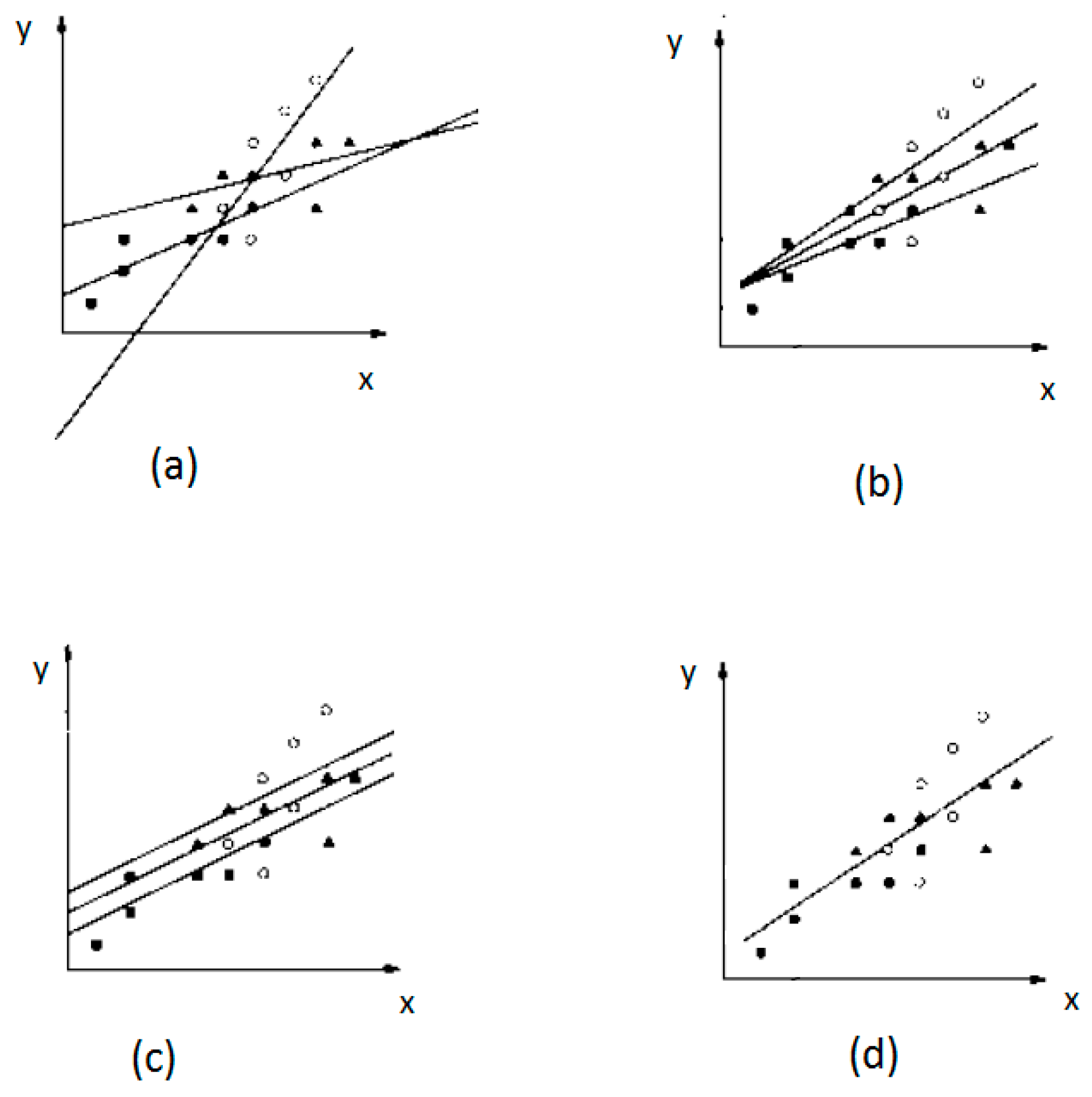
An adjusted mean is the mean dependent variable that would be expected or is predicted for each group, if the covariate variable mean is equal to the grand covariate mean. The grand covariate mean is a unique logσu and the adjusted fatigue life in each group is estimated according to this stress amplitude. In this way, for each group there is a unique point (logσu, logNj,adj). This value would be different in different groups, and these values can be used to compare the state of the regression lines to each other. According to adjusted means and slopes of regression lines, there are four types of regression line configurations, as shown in Figure 1 below.
By adjustment of the point and slope for each group, comparisons can be performed. As mentioned above, the purpose of the ANCOVA is to test the null hypothesis that two or more adjusted population means are equal. Alternatively, the purpose could be formulated as to test the equality of two or more regression intercepts. Under the assumption of parallel regression lines, the difference between intercepts must be equal to the difference between adjusted means. The formula for the computation of adjusted means is:
where is the adjusted mean for the j-th group; is the unadjusted mean (mean of fatigue life) for the j-th group; bw is the pooled within-group regression coefficient (for details see [5,11]); is the mean of the stress amplitude for the j-th group; is the mean of the logσij values.
3.2. Testing the Homogeneity of Regression Slopes
An assumption underlying the use of ANCOVA is that the population regression slopes are equal. If the slopes are not equal, the “Type of groups” effects differ at different levels of the stress amplitude; consequently, the adjusted stress amplitudes can be misleading because they do not convey this important information. When the slopes are the same, the adjusted means are adequate descriptive measures because the differences of the fatigue life are the same at different levels of the stress amplitude.
If the slopes for the populations in an experiment are equal, that is, , a reasonable way of estimating the value of this common slope from the samples is by computing an average of the sample b1 values:
where from Equation (5) we have:
The slope bw is the best estimate of the population slope β1, which is the slope assumed to be common to all groups. As long as , the estimate bw is a useful statistical value to use. Now the problem is to decide whether all groups have the same slope. The homogeneity of the regression F-test is designed to answer the question of the equality of the population slopes. The null hypothesis associated with this test is:
The steps involved in the computation of the test are described next:
Steps 1 and 2: Computation of within-group sum of squares and within-group residual sum of squares (SSresw)
Step 3: Computation of individual sum of squares residual (SSresi)
The third step involves the computation of the sum of squares residual for each group separately, and then adding these residuals to obtain the sum of the individual residual sum of squares (SSresj). The difference in the computations of SSresw and SSresj is that SSresw involves computing the residual sum of squares around the single bw value whereas SSresj involves the computation of the residual sum of squares around the bj values fitted to each group separately (Equation (13)).
Step 4: Computation of heterogeneity of slopes sum of squares
The discrepancy between SSresw and SSresi reflects the extent to which the individual regression slopes are different from the within-group slope bw; hence, the heterogeneity of slopes SS is “SShet = SSresw − SSresi”, see [5].
Step 5. Computation of F-ratio
The summary table for the F-test is as follows (Table 2). If the obtained F is equal to or greater than , then the null hypothesis is rejected.
In this method, diagnostic checking of the covariance model is based on residual analysis. Furthermore, the measure of uncertainty is not directly related to the uncertainty of the SN curve. The uncertainty of SN curves used in the next section has been evaluated by the maximum likelihood method (MLM) [2].
4. Reliability Assessment
The fatigue strength of metals is often assumed to follow the Basquin equation (the equation is based on fully reversed fatigue (R = −1), i.e., the mean value is zero) and is written [12]:
where N is the number of stress cycles to failure with constant stress ranges Δσ; K and m are material parameters dependent on the fatigue critical detail. The fatigue strength ΔσF may, e.g., be defined as the value of S for, e.g., ND = 2 × 10⁶ [7]. If one fatigue critical detail is considered, then the annual probability of failure is obtained from:
where P(fatigue failure in year t) is the probability of failure in year t and PCOL|FAT is the probability of collapse of the structure given fatigue failure—modeling the importance of the details/consequences of failure. The probability of failure in year t given survival up to year t is estimated by:
where the limit state equation is based on the application of SN curves and Miner’s rule for linear accumulation of fatigue damage, and by introducing stochastic variables accounting for uncertainties in fatigue loading and strength. Note that the probability of failure also depends on the repair and maintenance methods’ accuracy and protective methods that have been applied on the component. The design equation can be written as follows, if used in a deterministic code-based verification:
where ni,S represents the number of cycles per year at a specific stress level and TL is the design lifetime. It is assumed that for a wind turbine component, for a given fatigue life, the number of cycle according to the stress can be grouped as nσ, where the number of excitation at the specific stress range i is ni,S per year. In this paper, the Level II reliability method is used to estimate the reliability of the components [7]. The design parameter z is obtained from Equation (17), assuming that the fatigue partial safety factors are given. Consequently, the reliability equation is normalized and it became a function of the partial safety factors and presumed that the component is designed to the limit according to the design parameter z in the design equation.
For a deterministic design, the following partial safety factors are introduced [13]:
- a fatigue load partial safety factor multiplied by the fatigue stress ranges obtained by, e.g., rainflow counting.
- a fatigue strength partial safety factor. The design value of the fatigue strength is obtained by dividing the characteristic fatigue strength by .
The characteristic fatigue strength can be defined in various ways, namely based on:
- the mean minus two standard deviations of log K.
- the 5% quantile of log K, i.e., the mean minus 1.65 times the standard deviation of log K.
- the mean of log K.
The corresponding limit state equation to be used in the reliability analysis is written:
where XW is a stochastic variable modeling model uncertainty related to the determination of fatigue loads and XSCF is a stochastic variable modeling model uncertainty related to the determination of stresses given fatigue loads. In addition, Δ models model uncertainty related to Miner’s rule for linear damage accumulation [2]. In Equation (18), Δ, XW and XSCF are assumed to be log-normal distributed with mean values equal to 1 and coefficients of variation COVΔ, COVW and COVSCF, respectively, and can be written as following equation:
The coefficients of variation are estimated partly subjectively, but generally following the recommendations used as a basis for the material partial safety factors in IEC 61400-1, and also considering information from, e.g., [14]. The importance of the choices of the coefficients of variation is investigated by sensitivity analyses. It is noted that the reliability level obtained is in accordance with the target reliability corresponding to an annual probability failure of the order 5 × 10⁻⁴ (annual reliability index 3.3) [15]. In Table 3, the stochastic model is shown. It is noted that m and Δσf are correlated with statistical parameters extracted from [2]. The stochastic model is considered as representative for the fatigue strength represented by SN curves. It is assumed that the design lifetime is TL = 25 year [13].
If the SN curves are obtained by a limited number of tests, then statistical uncertainty has to be accounted for. Table 4 shows indicative values of for the target reliability index equal to 3.3 as a function of the total coefficient of variation of the fatigue load: . It is noted that more fatigue test data should be investigated to validate the indicative values in Table 4.
5. Results and Discussion
This section presents results obtained using representative fatigue test data from test specimens of cast components. The casted specimens are manufactured by two different manufacturing processes. The manufacturing processes are “sand casting” and “chill casting”. In this section, the ANCOVA method is used to compare the different test laboratories and different extractions of samples for the tests and obtaining the fatigue test data.
5.1. Comparison of Different Test Laboratories
The fatigue tests were carried out by four different test laboratories. Table 5 shows the number of tests in each group. The comparison between groups (Tests labs) was performed using sand casting results because there was only one group with chill casting. In this configuration, the run-out samples were considered as broken samples with very high cycles in order not to exclude them from the analysis. A summary of the ANCOVA calculations is shown in Table 6.
The value of bw shows that the stress amplitude and fatigue life were negatively correlated. First it was tested if the choice of test laboratory does not affect the fatigue test results.
The null hypothesis is: H0, the choice of test laboratory does not affect the fatigue test results.
The F-ratio is calculated according to Section 3. The study involves one covariate, four groups and 827 test results. The F-ratio calculation is summarized in Table 7.
The obtained F was then compared with the critical value of F with three and 822 degrees of freedom and a level of significance equal to 5%; F(0.05, 3,822) equals 2.62, and the null hypothesis of “The choice of test laboratory does not affect the fatigue test results” was rejected. Next, the homogeneity of the slopes of regression lines was considered, i.e., it was tested if the slopes of the different regression lines were equal. The null hypothesis is written: The summary of the calculation is shown in Table 8.
The critical value is F(0.05, 3, 821) = 2.62; hence, the null hypothesis was accepted. It was concluded that the slopes of the regression lines are similar. Figure 2 shows the results for the regression lines (note the results are normalized). It was seen that “Group 2” had the highest fatigue life and “Group 1” had the lowest fatigue life compared to the other testing places and the groups had the same slope.
5.2. Comparison of Different Cutting Facilities
The components from where samples were taken were cut up at different facilities. The cutting facilities were used to cut the sand casting samples after casting processes, and therefore they could be considered as a part of the manufacturing process for the casting samples. Table 9 shows the number of tests in each group. It is noted that the groups of cutting facilities are not the same as the groups of testing laboratories.
In this case, the comparison between groups was performed using sand casting and chill casting. The results of the ANCOVA for sand casting and chill casting are shown in Table 10 and Table 11, respectively.
The obtained F statistic was then compared with the critical value. In both casting methods, the null hypothesis of “The choice of cutting facilities does not affect the fatigue test results” was rejected. Next, the homogeneity of the regression test (slope of regression lines) was considered. The summaries of the calculation are shown in Table 12 and Table 13.
Based on Table 12 and Table 13, the null hypothesis is rejected and slopes of regression lines are not the same. Figure 3 and Figure 4 show the results for the regression lines of sand casting and chill casting, respectively (note the results are normalized).
According to Figure 3 and Figure 4, Group 2 has a different slope compared to the other groups, but the other groups are similar to each other. For sand casting, quite small differences between fatigue lives were obtained for cutting facilities 1, 3, 4 and 5. For chill casting, relatively larger differences in fatigue lives were obtained for cutting facilities 1, 4 and 5.
5.3. Reliability Analysis: Examples
In the following, the SN curves that were derived in the above sections are used for reliability analysis in a case study. The parameters used for analysis are listed in Table 14. By using the design Equation (17), the design values (z) are determined for each group, as shown in Table 15 and Table 16.
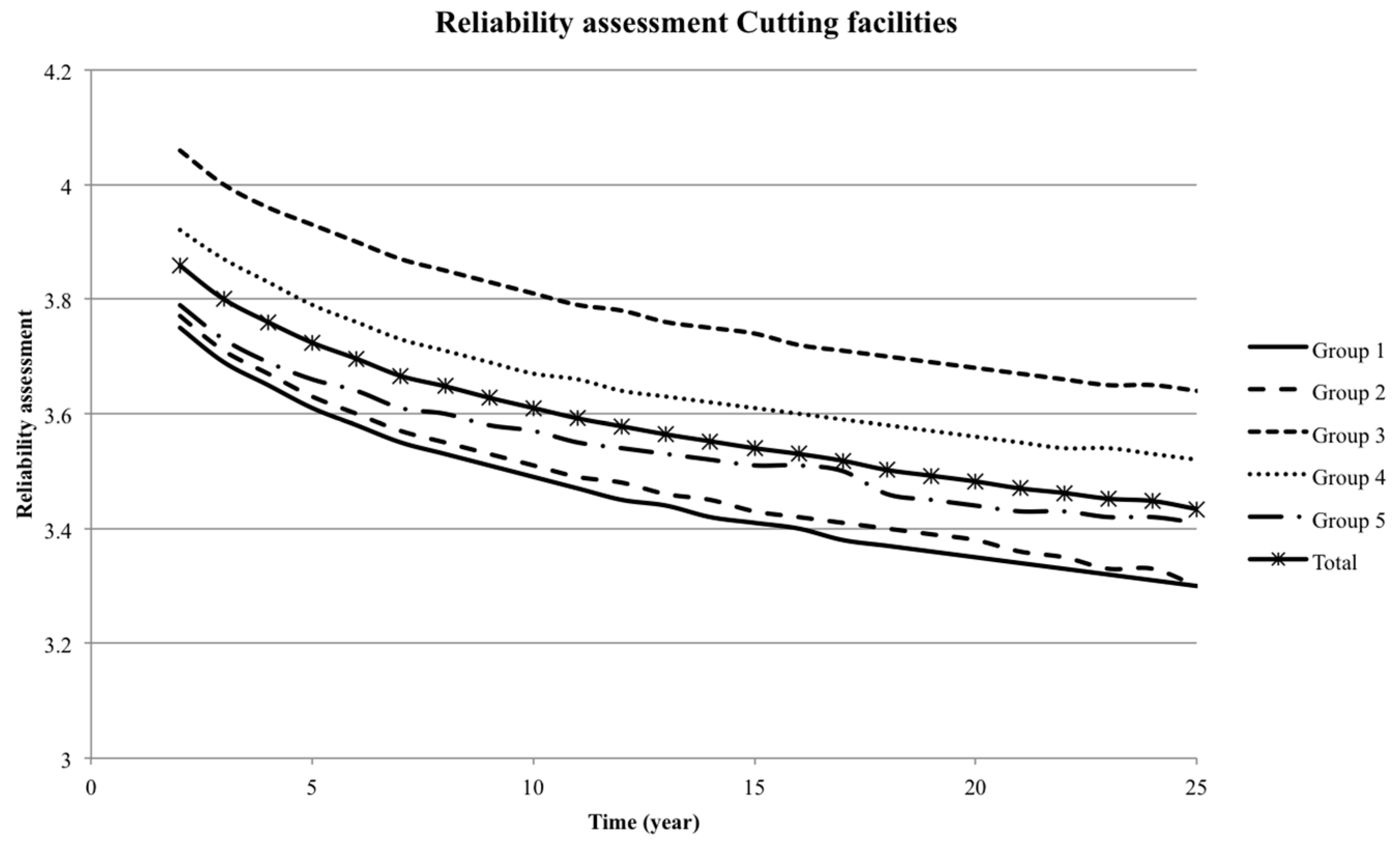
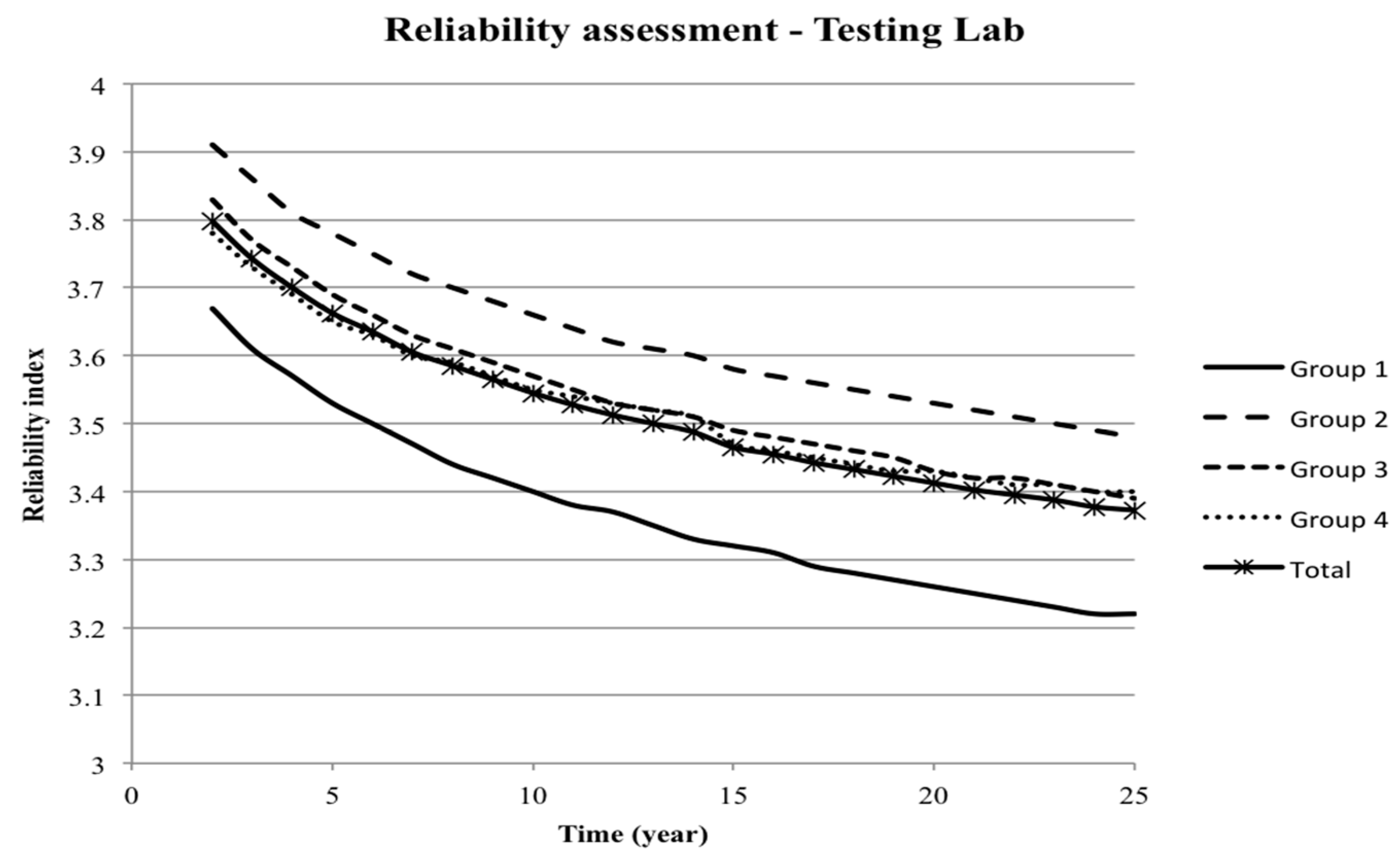
The reliability indices as a function of time for the groups of testing laboratories (Section 5.1) were estimated and are shown in Figure 5. Note that in this figure the annual reliability index is shown. The data from Group 2 result in the largest reliability level compared to the other groups. Moreover, the annual reliability index for cutting samples groups (Section 5.2) is shown in Figure 6. It is seen that the annual reliability indices at the end of the lifetime are of the order of 3.3, corresponding to the target annual reliability index = 3.3.
6. Conclusions
In this paper, the ANCOVA method is used to compare different groups related to the manufacturing process and associated quality control of cast components. The ANCOVA method is applied for fatigue failure data. Test data is used to illustrate the implementation of the ANCOVA method. The different test laboratories and cutting facilities are compared to each other. The results obtained from the ANCOVA analysis can be used for decision-making on which test laboratories and cutting facilities should be included in a statistical analysis in order to make sure that the statistical analyses are performed on data from a statistically homogeneous population. More parameters can be included, if relevant.
Further, it is presented how to apply the statistical results from the ANCOVA analysis to estimate the reliability for generic cases, and to assess the required safety factors for deterministic design such that a given target reliability level is obtained. It is noted that more data and more example structures are needed to perform a more general reliability-based calibration of safety factors with the proposed approach.
Acknowledgments
The work is supported by the Strategic Research Center “REWIND—Knowledge based engineering for improved reliability of critical wind turbine components”, the Danish Research Council for Strategic Research, grant No. 10-093966. Fatigue test data is provided by Vestas Wind Systems A/S, Denmark.
Author Contributions
Hesam Mirzaei Rafsanjani contributed to defining the overall problem and proposed the core scientific idea to solve it. Hesam Mirzaei Rafsanjani established the ANCOVA analysis of SN curve models for fatigue samples that has been tested in the RISØ center (DTU Roskilde campus) and they had been provided by the industrial partner of the project. The test samples provided by “Asger Sturlason” and tests were carried out in the RISØ center by “Søren Fæster”. Hesam Mirzaei Rafsanjani conducted all the numerical simulations included in the paper and interpreted all the results with the help of the supervisor (co-author John Dalsgaard Sørenesen). Further, Hesam Mirzaei Rafsanjani wrote the manuscript and revised it according to co-author comments.
Conflicts of Interest
The authors declare no conflict of interest.
References
- Tavner, P.J.; Greenwood, D.M.; Whittle, M.W.G.; Gindele, R.; Faulstich, S.; Hahn, B. Study of weather and location effects on wind turbine failure rates. Wind Energy 2012, 16, 175–187. [Google Scholar] [CrossRef]
- Rafsanjani, H.M.; Sørensen, J.D. Reliability analysis of fatigue failure of cast components for wind turbines. Energies 2015, 8, 2908–2923. [Google Scholar] [CrossRef]
- Rafsanjani, H.M.; Sørensen, J.D. Stochastic models of defects in wind turbine drivetrain components. In Multiscale Modeling and Uncertainty Quantification of Materials and Structures; Papadrakakis, M., Stefanou, G., Eds.; Springer International Publishing: Cham, Switzerland, 2014; pp. 287–298. [Google Scholar]
- Shirani, M.; Härkegård, G. Damage tolerant design of cast components based on defects detected by 3D X-ray computed tomography. Int. J. Fatigue 2012, 41, 188–198. [Google Scholar] [CrossRef]
- Huitema, B.E. The Analysis of Covariance and Alternatives Statistical Methods for Experiments, Quasi-Experiments, and Single-Case Studies; Wiley: Hoboken, NJ, USA, 2011. [Google Scholar]
- Sørensen, J.D.; Toft, H.S. Probabilistic design of wind turbines. Energies 2010, 3, 241–257. [Google Scholar] [CrossRef]
- Sørensen, J.D.; Toft, H.S. Safety Factors—IEC 61400-1 ed.; 4—Background Document, DTU Wind Energy- E-Report-0066 (EN); DTU: Copenhagen, Denmark, 2014. [Google Scholar]
- Madesn, H.O.; Krenk, S.; Lind, N.C. Methods of Structural Safety; Dover Publications: Mineola, NY, USA, 1986. [Google Scholar]
- Zimmerman, D.W. A note on interpretation of the paired-samples t test. J. Educ. Behav. Stat. 1997, 22, 349–360. [Google Scholar] [CrossRef]
- Ayyub, B.M.; McCuen, R.H. Probability, Statistics, and Reliability for Engineers and Scientists, 2nd ed.; CRC/Chapman & Hall: Boca Raton, FL, USA, 2002. [Google Scholar]
- Montgomery, D.C. Design and Analysis of Experiments, 8th ed.; Wiley: Hoboken, NJ, USA, 2013. [Google Scholar]
- Silk, J. Analysis of Covariance and Comparison of Regression Lines; University of East Anglia: Norwich, UK, 1979. [Google Scholar]
- Sørensen, J.D. Reliability assessment of wind turbines. In Proceedings of the 12th International Conference on Applications of Statistics and Probability in Civil Engineering ICASP12, Vancouver, BC, Canada, 12–15 July 2015. [Google Scholar]
- Fatigue Design of Offshore Steel Structures; DNV-RP-C203; Det Norske Veritas: Høvik, Norway, 2010.
- Wind Turbine—Part 1: Design Requirements; IEC 61400; International Electrotechnical Commission (IEC): Geneva, Switzerland, 2015.
Figure 1.
Relation between regression lines. (a) Completely different; (b) intercept (same intercepts); (c) parallel (same slope but without intercept); and (d) coincidence (exactly same lines) [12].
Figure 1.
Relation between regression lines. (a) Completely different; (b) intercept (same intercepts); (c) parallel (same slope but without intercept); and (d) coincidence (exactly same lines) [12].

Figure 2.
Comparison of “testing laboratories” on logarithmic scale.

Figure 3.
Comparison of “cutting facilities” on logarithmic scale for sand casting.
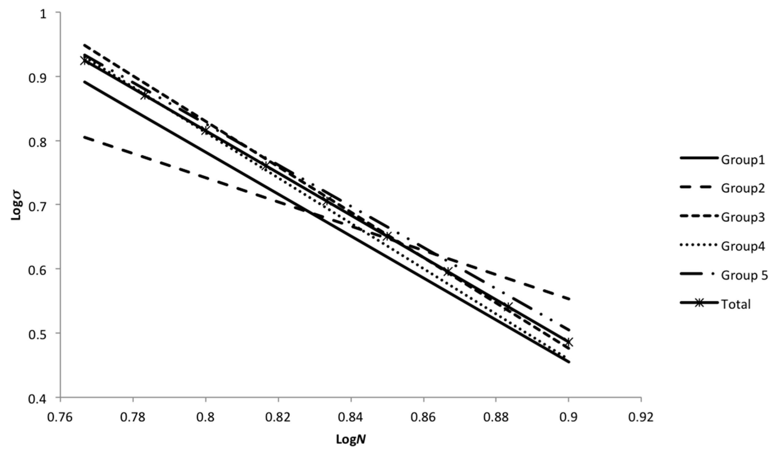
Figure 4.
Comparison of “cutting facilities” on logarithmic scale for chill casting.
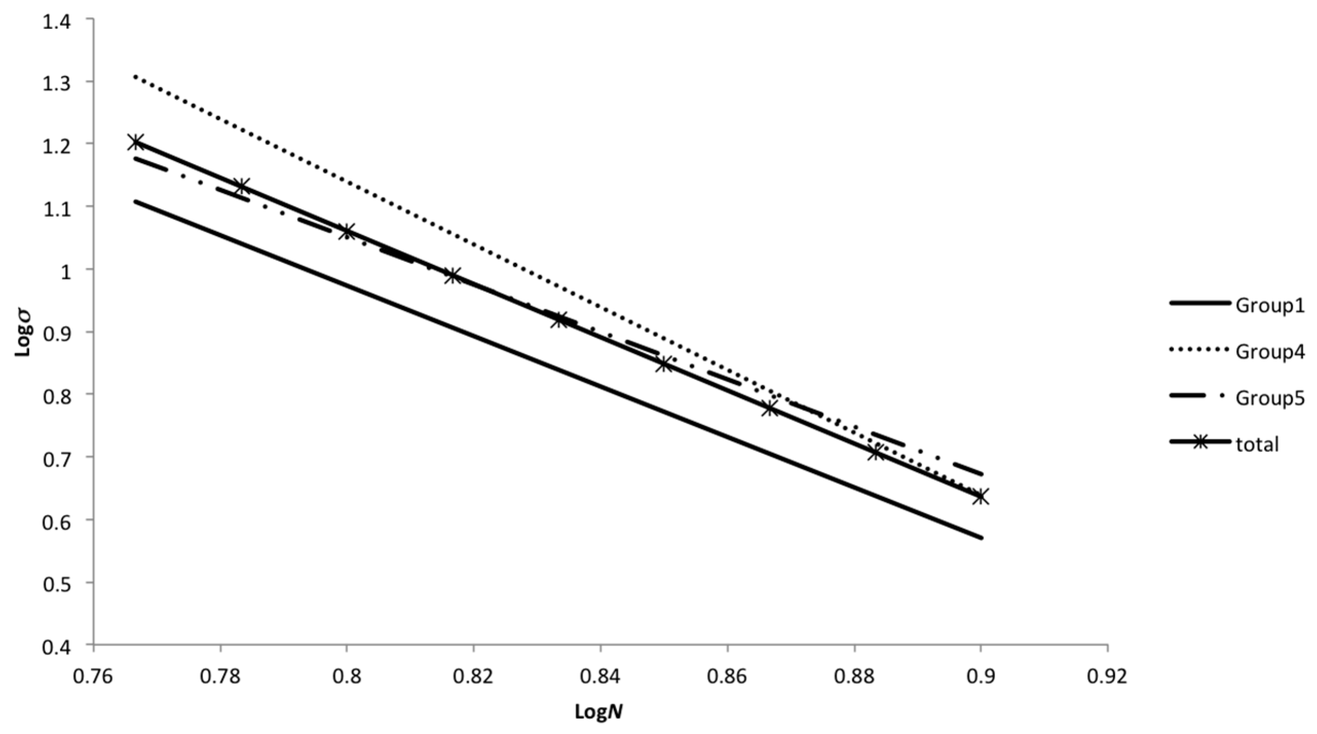
Figure 5.
Annual reliability index for different groups based on test laboratories categories (sand casting).
Figure 5.
Annual reliability index for different groups based on test laboratories categories (sand casting).

Figure 6.
Annual reliability index for different groups based on cutting facilities categories (sand casting).
Figure 6.
Annual reliability index for different groups based on cutting facilities categories (sand casting).


Table 1.
Computation table for analysis of variance test. SS: Sum of square; DF: degrees of freedom and MS: mean square.
Table 1.
Computation table for analysis of variance test. SS: Sum of square; DF: degrees of freedom and MS: mean square.
| Source of Variation | Sum of Square | Degrees of Freedom | Mean Square |
|---|---|---|---|
| Between | k − 1 | ||
| Within | M − k | ||
| Total | M − 1 | - |
Table 2.
Computation table for the heterogeneity of the slope.
| Source of Variation | Sum of Square | Degrees of Freedom | Mean Square | F |
|---|---|---|---|---|
| Heterogeneity of slopes | SShet | k − 1 | ||
| Individual residual (resi) | SSresi | M − 2k | - | |
| Within residual (resw) | SSresw | M − k − 1 | - | - |
Table 3.
Stochastic model of fatigue strength based on SN curves.
| Variable | Definition | Distribution | Expected Value | Coefficient of Variation |
|---|---|---|---|---|
| Δ | Model uncertainty related to Miner’s rule | LN * | 1 | COVΔ = 0.3 |
| XSCF | Model uncertainty related to determination of stresses given fatigue load | LN | 1 | COVSCF |
| XW | Model uncertainty related to determination of fatigue loads | LN | 1 | COVW |
| m | Slope SN curve (Statistical uncertainty) | N ** | Extracted from test results, [2] | |
| Δσf (Mpa) | Fatigue Strength (Statistical uncertainty) | N | Extracted from test results, [2] | |
* Log-Normal Distribution; ** Normal Distribution.
Table 4.
Indicative partial safety factors as function of COV for fatigue load.
| / | 0.00 | 0.05 | 0.10 | 0.15 | 0.20 | 0.25 | 0.30 |
| 3,3 (5 × 10⁻⁴) | 1.62 | 1.63 | 1.67 | 1.74 | 1.83 | 1.95 | 2.11 |
Table 5.
Number of test results by test laboratories.
| Testing Laboratories | Sand Casting | Chill Casting | Total | ||
|---|---|---|---|---|---|
| Broken | Run-out | Broken | Run-out | ||
| Group 1 | 28 | 2 | - | - | 30 |
| Group 2 | 609 | 109 | 302 | 107 | 1127 |
| Group 3 | 57 | 3 | - | - | 60 |
| Group 4 | 19 | - | - | - | 19 |
| Summation | 713 | 114 | 302 | 107 | 1236 |
Table 6.
Summary of calculations for test laboratories comparison. SS: Sum of squares.
| Parameter | Value | Parameter | Value |
|---|---|---|---|
| Syy | 574 | SSresw | 196 |
| SSrest | 206 | SSAT | 9.6 |
| SSregw | 377 | bw | −8.9 |
Table 7.
Computation table for the test laboratories comparison.
| Source of Variation | Sum of Square | Degrees of Freedom | Mean Square | F | p-Value |
|---|---|---|---|---|---|
| Adjusted (AT) | 9.56 | 3 | 3.2 | 13.3 | 0.00 |
| Error (resw) | 196 | 822 | 0.2 | ||
| Total residual (rest) | 205 | 825 | - |
Table 8.
Computation heterogeneity of slopes for test laboratories comparison.
| Source of Variation | Sum of Square | Degrees of Freedom | Mean Square | F | p-Value |
|---|---|---|---|---|---|
| Heterogeneity of slopes | 1.2 | 3 | 0.41 | 1.71 | 0.16 |
| Individual residual (resi) | 194 | 821 | 0.24 | ||
| Within residual (resw) | 196 | 824 | - |
Table 9.
Number of test results by cutting facilities.
| Cutting Facilities | Sand Casting | Chill Casting | Total | ||
|---|---|---|---|---|---|
| Broken | Run-out | Broken | Run-out | ||
| Group 1 | 107 | 8 | 96 | 3 | 214 |
| Group 2 | 18 | 3 | - | - | 21 |
| Group 3 | 95 | 14 | - | - | 109 |
| Group 4 | 148 | 26 | 107 | 53 | 334 |
| Group 5 | 345 | 63 | 99 | 51 | 558 |
| Summation | 713 | 114 | 302 | 107 | 1236 |
Table 10.
Computation table for the cutting facilities based on sand casting method.
| Source of Variation | Sum of Square | Degrees of Freedom | Mean Square | F | p-Value |
|---|---|---|---|---|---|
| Adjusted (AT) | 16 | 4 | 3.8 | 16.3 | 0.00 |
| Error (resw) | 191 | 821 | 0.2 | - | - |
| Total residual (rest) | 206 | 825 | - | - | - |
Table 11.
Computation table for the cutting facilities based on chill casting method.
| Source of Variation | Sum of Square | Degrees of Freedom | Mean Square | F | p-Value |
|---|---|---|---|---|---|
| Adjusted (AT) | 42 | 2 | 21.0 | 111 | 0.00 |
| Error (resw) | 77 | 405 | 0.19 | - | - |
| Total residual (rest) | 119 | 407 | - | - | - |
Table 12.
Computation heterogeneity of slopes for cutting facilities based on sand casting.
| Source of Variation | Sum of Square | Degrees of Freedom | Mean Square | F | p-Value |
|---|---|---|---|---|---|
| Heterogeneity of slopes | 3.0 | 4 | 0.75 | 3.28 | 0.011 |
| Individual residual (resi) | 181 | 817 | 0.23 | - | - |
| Within residual (resw) | 190 | 821 | - | - | - |
Table 13.
Computation heterogeneity of slopes for cutting facilities based on chill casting.
| Source of Variation | Sum of Square | Degrees of Freedom | Mean Square | F | p-Value |
|---|---|---|---|---|---|
| Heterogeneity of slopes | 3.4 | 2 | 1.68 | 9.24 | 0.000 |
| Individual residual (resi) | 73.2 | 403 | 0.18 | - | - |
| Within residual (resw) | 76.6 | 405 | - | - | - |
Table 14.
Statistical parameters for reliability assessment of samples.
| COVΔ | COVSCF | COVW | |||
|---|---|---|---|---|---|
| 0.3 | 0.1 | 0.05 | 0.11 | 0.95 | 1.75 |
Table 15.
Design values (z) for testing lab groups (obtained from Equation (17)).
| Groups | Group 1 | Group 2 | Group 3 | Group 4 |
|---|---|---|---|---|
| z-value | 0.228 | 0.203 | 0.214 | 0.210 |
Table 16.
Design values (z) for cutting facilities groups (obtained from Equation (17)).
| Groups | Group 1 | Group 2 | Group 3 | Group 4 | Group 5 |
|---|---|---|---|---|---|
| z-value | 0.226 | 0.510 | 0.178 | 0.184 | 0.214 |
© 2017 by the authors. Licensee MDPI, Basel, Switzerland. This article is an open access article distributed under the terms and conditions of the Creative Commons Attribution (CC BY) license (http://creativecommons.org/licenses/by/4.0/).
Share and Cite
MDPI and ACS Style
Mirzaei Rafsanjani, H.; Sørensen, J.D.; Fæster, S.; Sturlason, A. Fatigue Reliability Analysis of Wind Turbine Cast Components. Energies 2017, 10, 466. https://doi.org/10.3390/en10040466
AMA Style
Mirzaei Rafsanjani H, Sørensen JD, Fæster S, Sturlason A. Fatigue Reliability Analysis of Wind Turbine Cast Components. Energies. 2017; 10(4):466. https://doi.org/10.3390/en10040466
Chicago/Turabian StyleMirzaei Rafsanjani, Hesam, John Dalsgaard Sørensen, Søren Fæster, and Asger Sturlason. 2017. "Fatigue Reliability Analysis of Wind Turbine Cast Components" Energies 10, no. 4: 466. https://doi.org/10.3390/en10040466
Note that from the first issue of 2016, this journal uses article numbers instead of page numbers. See further details here.