
A 3-D Coupled Magneto-Fluid-Thermal Analysis of a 220 kV Three-Phase Three-Limb Transformer under DC Bias

School of Electrical Engineering, Wuhan University, No. 8, South Road of Eastern Lake, Wuhan 430072, China
*
Author to whom correspondence should be addressed.
Energies 2017, 10(4), 422; https://doi.org/10.3390/en10040422
Submission received: 11 January 2017
/
Revised: 28 February 2017
/
Accepted: 20 March 2017
/
Published: 23 March 2017
Abstract
:This paper takes a typical 220 kV three-phase three-limb oil-immersed transformer as an example, this paper building transient field-circuit coupled model and 3D coupled magneto -fluid-thermal model. Considering a nonlinear B–H curve, the magneto model uses the field-circuit coupled finite element method (FEM) to calculate the magnetic flux distribution of the core and the current distribution of the windings when the transformer is at a rated current and under direct current (DC) bias. Taking the electric power losses of the core and windings as a heat source, the temperature inside the transformer and the velocity of the transformer oil are analyzed by the finite volume method (FVM) in a fluid-thermal field. In order to improve the accuracy of the calculation results, the influence of temperature on the electrical resistivity of the windings and the physical parameter of the transformer oil are taken into account in the paper. Meanwhile, the convective heat transfer coefficient of the FVM model boundary is determined by its temperature. By iterative computations, the model is updated according to the thermal field calculation result until the maximum difference in hot spot temperature between the two adjacent steps is less than 0.01 K. The result calculated by the coupling method agrees well with the empirical equation result according to IEC 60076-7.
1. Introduction
As one of the most important pieces of equipment in the electrical power system, transformers are numerous in quantity and complicated in structure, directly determining the reliability and security of a power supply. Hot-spot temperature is one of the most important factors that influence the operational status, physical conditions, and insulation life of transformers, so it has become a hot topic among transformer manufacturers, electrical departments, and research institutes [1,2,3].
The direct current (DC) bias phenomenon occurs when DC flows into the windings of a transformer through the neutral point, which is an abnormal workstation. There are two main reasons that give rise to DC bias: one is the mono-polar ground circuit operation mode or the bipolar asymmetrical operation mode of the HVDC (High Voltage Direct Current Transmission) transmission system, and the other is geomagnetically induced current (GIC), which is caused by the interaction between the geomagnetic field and the dynamic movement of ionic wind. The change in geomagnetic field produces an electric potential gradient, which brings low-frequency induction current. It is identified as DC because its frequency is very low [4,5].
DC bias causes an increase in magnetizing current, harmonics leakage magnetic flux, and thus losses, which leads to hot spot overheating and insulation aging. The temperature rises of the core and windings directly affect the durability and ultimate life of the transformer, so it is important to predict the transformer hot spot temperature rise when it is under DC bias [6,7].
In order to avoid the oil-flow electrification phenomenon, oil-immersed natural-air cooled type (ONAN) is commonly used in large-capacity transformers. This paper presents an accurate calculation for hot spot temperature-rise estimations in an 180 MVA/220 kV three-phase three-limb ONAN transformer. First, the power losses when the transformer is at a rated current and under DC bias are computed using a transient field-circuit coupled FEM model. Then, the thermal-fluid-coupled FVM model is activated to calculate the temperature and velocity distribution inside the transformer [8]. The above models take oil changes, boundary changes, and loss variation with temperature into account. To verify the accuracy of the proposed model, results are calculated via empirical formula according to IEC 60076-7, and simulation results are compared.
2. Theory and Equations
2.1. Circuit Model
The current distribution in windings is calculated by a circuit-field coupled model, which is described by the magnetic flux linkage equation, the electromotive force equation, and the transient response equation:
where is the winding flux linkage vector, and Ls stands for the static inductance matrix; I represents the exciting current; E is the electromotive force; LT is the transient inductance matrix.
2.2. Electromagnetic Field Equations
The heat sources inside the transformer mainly come from the transformer core and windings when it is running, which can be computed by electromagnetic analysis. According to Maxwell’s equation, the governing equation of quasi-static magnetic field problem based on magnetic vector potential can be expressed as [9]:
where μ is the magnetic permeability; σ is the conductivity; A stands for the magnetic vector potential; Js represents the current density vector.
2.3. Fluid-Thermal Field Equations
Taking the power losses derived from electromagnetic analysis as the heat source of thermal-fluid analysis, a mathematical model of the transformer internal oil flow based on the heat transfer theory and finite volume method was established. In consideration of the parameters of oil, the following assumptions were made in the FVM model:
- (1)
- oil flow inside the transformer is laminar flow;
- (2)
- oil is ideally incompressible Newtonian fluid.
The transformer internal oil flow can be described by the mass conservation equation, the energy conservation equation, and the momentum conservation equation [10,11]:
where ρ is the density, w is fluid velocity; F stands for the body force vector; p represents the pressure, and u denotes the dynamic viscosity; k is thermal conductivity, and c is the specific heat; T represents the temperature; q indicates volumetric heat source inside the transformer.
The heat dissipate in air though the tank and radiator. The external heat convection is described by following equations: [12,13].
where h is the convective heat transfer coefficient; S stands for the heat dissipating dimension of the transformer tank and radiator; Ts represents the temperature of transformer tank and radiator; Tf stands for ambient temperature; k is the thermal conductivity of air; l is the characteristic length; Nu is the Nusselt number.
According to heat transfer theory, the Nusselt number can be analyzed by the following equations.
where Gr is the Grashof number; g is the gravitational acceleration; β is the expansion coefficient; L is the feature size, and v is the kinematic viscosity; Pr is the Prandtl number, μ is the viscosity coefficient, and c is the specific heat capacity; k is the thermal conductivity; Ra is the Rayleigh number; a and b are constants dependent of the system.
2.4. Magneto-Fluid-Thermal Coupling Method
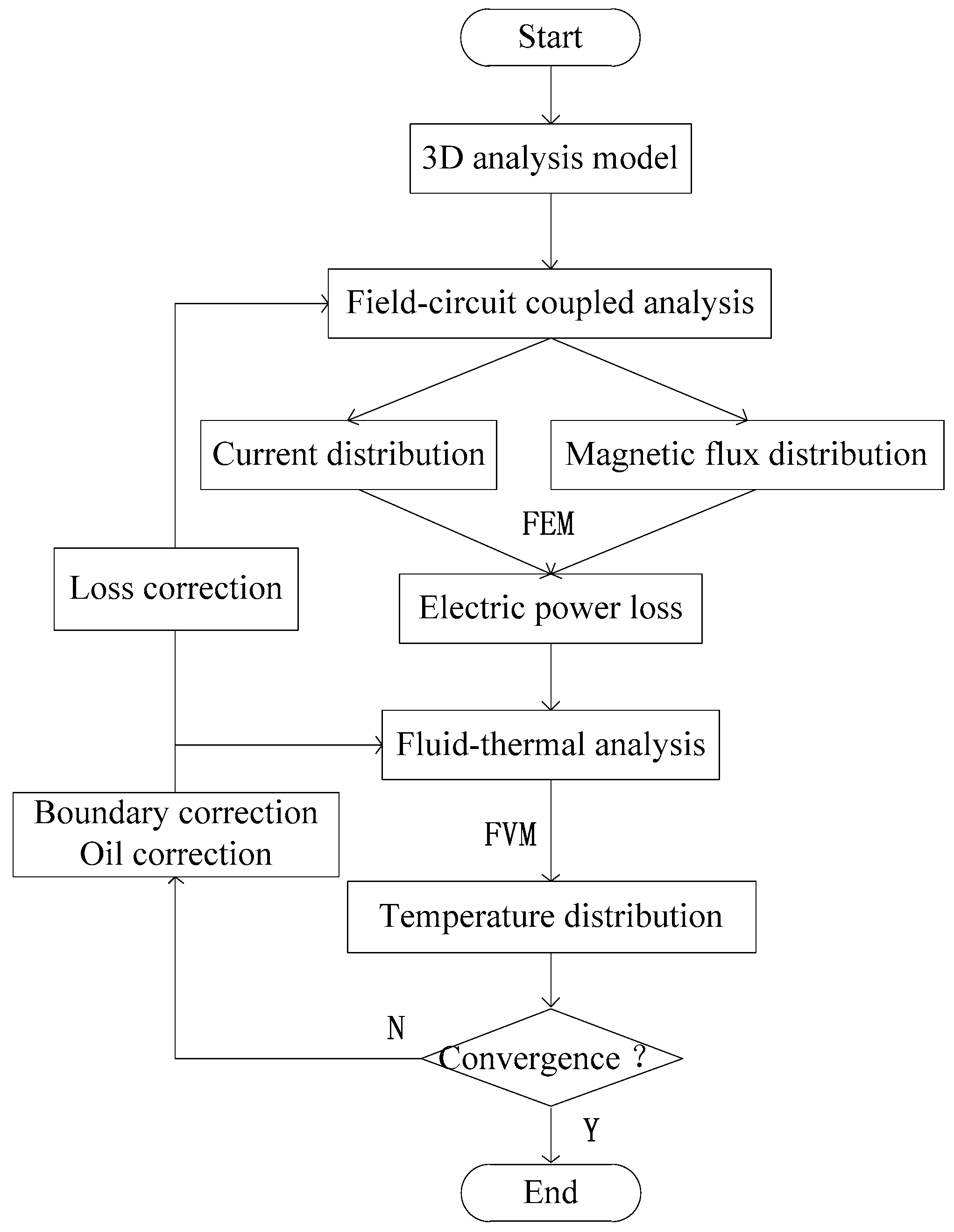
The flowchart of the 3-D coupled magneto-fluid-thermal field analysis is shown in Figure 1. The electric power loss of the core and windings are derived from harmonic magnetic analysis. Taking these losses as the heat sources of fluid-thermal analysis, the temperature distribution inside the transformer, especially the temperature of the high-voltage (HV) and medium-voltage (MV) windings, can be obtained. The electric power losses of the coils, the parameters of oil, and the convective heat transfer coefficient of the boundary will be updated in accordance to the thermal field calculation result until the maximum difference in temperature between the two adjacent steps is less than 0.01 K.
In consideration of the winding resistivity changes with temperature, in order to save computation time, the power losses of the windings are corrected by the following equation:
where P0 represents the winding losses at temperature T0; T is the windings temperature; α represents temperature coefficient of copper conductor, set to be 0.00393 in this paper.
In order to ensure the accuracy of fluid-thermal analysis, all oil properties were allowed to change with temperature. The physical parameters of the transformer oil are shown in Table 1.
3. Calculation of Three-Phase Three-Limb Transformer
3.1. The 220 kV Three-Phase Three Limb Transformer
A 3D numerical simulation using a commercial tool (ANSYS v15.0.) was conducted in this study. The 220 kV three-phase three-limb transformer analyzed in this paper consists of a 19 layer planar laminated core and 18 windings. Each limb is surrounded by six concentric windings: one layer of low-voltage (LV) winding, two layers of MV winding, and three layers of HV winding in turn from inside to outside. Windings are separated by vertical oil ducts. Each winding is composed of a set of several horizontal oil ducts, which separate the discs of copper coils from one another. In order to investigate the convective heat transfer process inside the transformer, vertical oil ducts between windings are considered. For the sake of saving computing time, the horizontal oil ducts between coils are ignored. The internal structure of the three-phase three-limb transformer is shown in Figure 2a. There are four oil tubes on both sides of the tank, and each oil tube is connected to two sets of radiators. The radiators are simplified down to the convective heat transfer coefficient of the oil tube surface. The external structure of the three-phase three-limb transformer is shown in Figure 2b.
The basic data of the transformer model are shown in Table 2.
3.2. Circuit-Field Coupled Analysis
The circuit-field coupling method proposed is used to calculate the current distribution of the 220 kV three-phase three-limb transformer. Because the core cannot form a loop for windings’ magnetic flux, the three-phase three-limb transformer is relatively insensitive to the DC bias current [6,7]. The exciting current is not distorted when the DC current is flowing into the transformer windings: the harmonic current distribution, except for the DC component, remains the same. The load current and operational states of transformers in practice are complicated. In order to simplify the calculation, the following assumptions are made:
- (1)
- HV windings and MV windings are at a rated current;
- (2)
- LV windings are no-load;
- (3)
- 20 A DC current flows into HV windings through the neutral point.
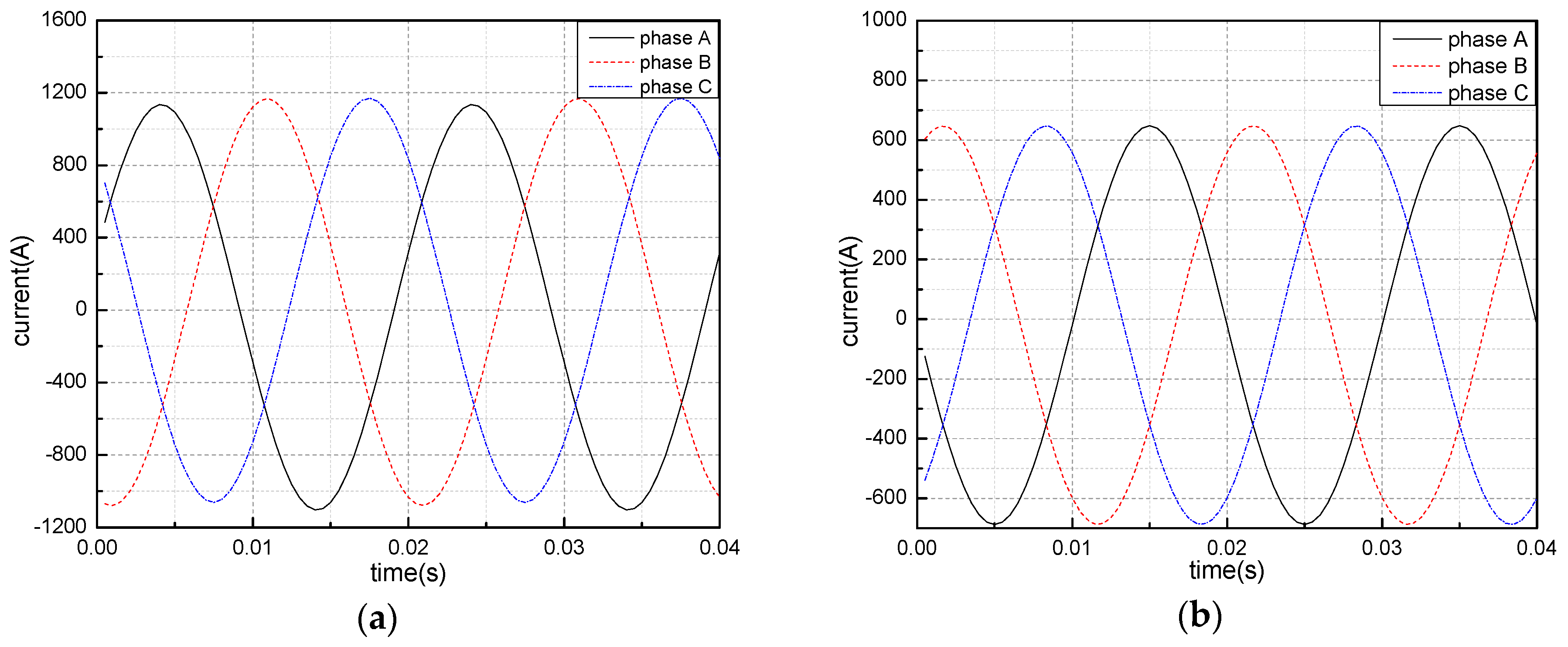
The current of MV windings and HV windings used in circuit-field coupled analysis are shown in Figure 3.
3.3. Electromagnetic Field Analysis
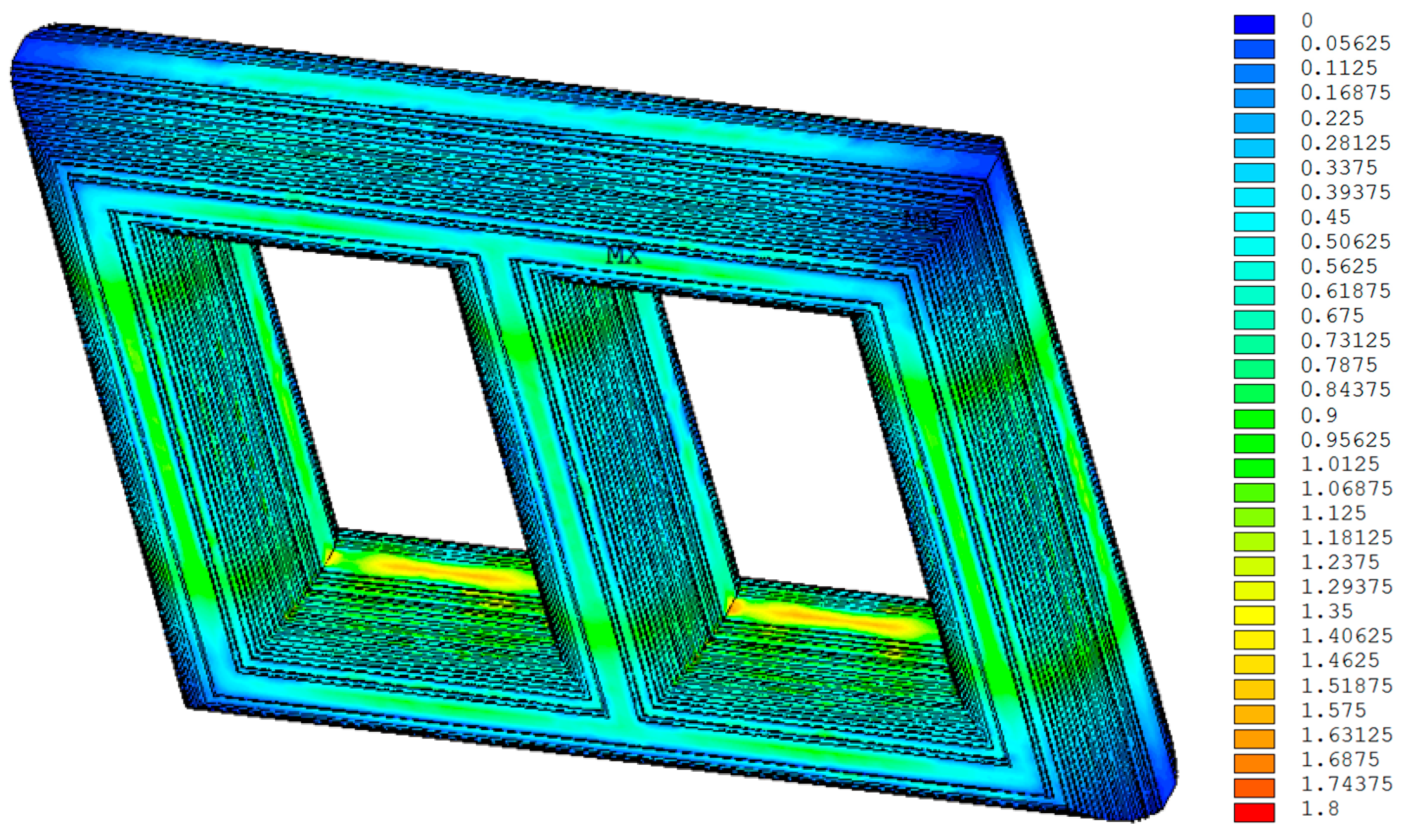
The magnetic performance of the three-phase three-limb transformer can be analyzed by the finite element method, and the result of the magnetic field is presented in Figure 4. The maximum magnetic flux density is about 1.7 T at the central part of the transformer cores if the computational error of the results at the core joints due to model structure and grid discretization are ignored.
For 30ZH100 silicon steel sheet, the unit power loss is about 0.98 W/kg when the maximum magnetic flux density is 1.7 T, and the core loss can then be derived from multiplying the core weight. Meanwhile, the power losses of the windings are calculated by electromagnetic analysis with a rated current and DC bias current.
3.4. Fluid-Thermal Field Analysis
Based on the heat source derived from the former analysis, the temperature distribution inside the transformer can be investigated by FVM in a fluid-thermal field. Because of the high viscosity and relatively low Rayleigh number (Ra ≤ 109) of oil flow, the laminar flow will be the main form of convection of the transformer oil.
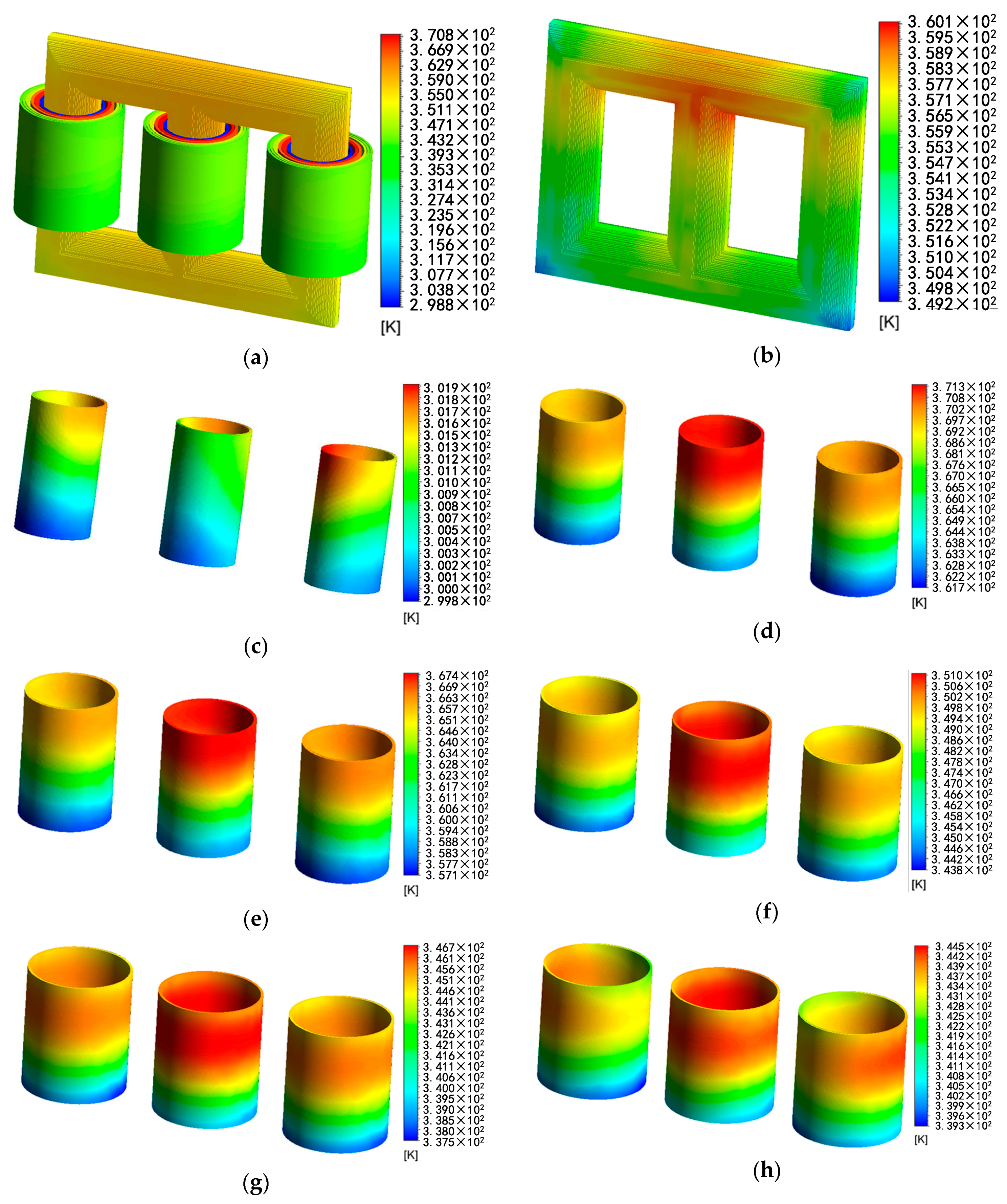
In order to improve the calculation efficiency, the radiators connected to the oil tube are simplified: the heat transfer coefficient of the oil tube is corrected according to the area of the corrugated sheet. The ambient temperature is set to 293.15 K. Taking the oil changes, the heat transfer coefficient changes, and the loss changes with temperature into consideration, the temperature distribution inside the transformer is investigated by fluid-thermal analysis. By iterative calculations, the model is updated according to the thermal field calculation result until the maximum difference in hot spot temperature between the two adjacent steps is less than 0.01 K. The results of fluid-thermal analysis are shown in Figure 5.
The transformer hot-spot temperature is 371.3 K and located at the upper part of the inner medium voltage windings, as shown in Figure 5d. For the transformer core, the maximum temperature is 360.1 K and located at the upper part of the B phase core limb, as shown in Figure 5a. The temperature distribution of the HV windings is shown in Figure 5f,g. The maximum temperature of the HV windings is 351.0 K. The temperature rise of the LV windings is relatively small because there is no load current.
The velocity distribution of the transformer oil inside the three-phase three-limb transformer is shown in Figure 6, which shows that the oil velocity near the upper part of the transformer core is much larger due to the higher temperature. The maximum velocity is 3.107 × 10⁻² m/s, which appears near the upper part of the oil tube, so the outside radiator has a great influence on the cooling system. The maximum velocity inside the tank is about 2.8 × 10⁻² m/s, located near the upper windings’ end. Convection plays an important role in the process of thermal dissipation. Hence, the optimal design of the oil tube and the horizontal oil ducts between coils are crucial for the temperature rise control of the transformer. Here are some suggestions for the optimization of the transformer cooling system:
- (1)
- For the ONAN transformer, the surface area of the outside radiator should be as large as possible;
- (2)
- The design of the windings should make sure the vertical oil duct is large enough for the oil flow.
According to IEC 60076-7, the hot-spot temperature of the transformer can be calculated by the ambient temperature, the top-oil temperature rise in the tank, and the temperature difference between the hot-spot and the top-oil in the tank [14]. The hot-spot temperature rise calculated via empirical formula is 80.1 K, which is in accordance with the results obtained by coupling analysis (the hot spot temperature derived from the proposed model is 77.8 K).
4. Conclusions
This paper focuses on the temperature distribution inside the three-phase three-limb transformer when it is under DC bias and puts forward an effective calculation method. The current distribution in the windings is calculated by coupled field-circuit analysis. In addition, the heat dissipation process and temperature distribution are analyzed via 3-D coupled magneto-fluid-thermal field analysis. Influences of temperature on coil loss, the physical parameters of the transformer oil, and the heat transfer coefficient of the boundary are taken into account to improve computational accuracy. The hot-spot temperature of the 220 kV ONAN three-phase three-limb transformer obtained by the coupling method discussed in this paper shows good agreement with the result acquired according to the IEC 60076-7 standard. Based on the calculation results, optimization of the transformer cooling system is put forward in this paper.
Acknowledgments
This article is supported by the National Engineering Laboratory for Ultra High Voltage Engineering Technology (Kunming, Guangzhou) (CSGTRC[2015]Q1543B14).
Author Contributions
Ruohan Gong and Jiangjun Ruan conceived and designed the models; Jingzhou Chen and Jian Wang performed the calculations; Yu Quan and Shuo Jin analyzed the data; Ruohan Gong wrote the paper.
Conflicts of Interest
The authors declare no conflict of interest.
References
- Zhang, Y.J.; Ruan, J.J.; Huang, T.; Yang, X.P.; Zhu, H.Q.; Yang, G. Calculation of temperature rise in air-cooled induction motors through 3-D coupled electromagnetic fluid-dynamic and thermal finite-element analysis. IEEE Trans. Magn. 2012, 48, 1047–1050. [Google Scholar] [CrossRef]
- Jahromi, A.; Piercy, R.; Cress, S.; Service, J.; Fan, W. An approach to power transformer asset management using health index. IEEE Electr. Insul. Mag. 2009, 25, 20–34. [Google Scholar] [CrossRef]
- Bicen, Y.; Cilliyuz, Y.; Aras, F.; Aydugan, G. An assessment on aging model of IEEE/IEC standards for natural and mineral oil-immersed transformer. In Proceedings of the IEEE International Conference on Dielectric Liquids, Trondheim, Norway, 26–30 June 2011; pp. 1–4. [Google Scholar]
- Li, C.Y. Effect of DC monopole operation on AC transformers. East China Electr. Power 2005, 33, 52–54. [Google Scholar]
- Price, P.R. Geomagnetically induced current effects on transformers. IEEE Trans. Power Deliv. 2002, 17, 1002–1008. [Google Scholar] [CrossRef]
- Li, Z.; Yun, Y.X. Harmonic distortion feature of AC transformers caused by DC bias. Power Syst. Prot. Control 2010, 34, 52–54. [Google Scholar]
- Li, X.P.; Wen, X.S.; Fan, Y.D.; Zhang, Y.; Lan, L.; Chen, C.X. Computation of Exciting Current and Harmonic for Three-phase and Three Limbs Transformer Under DC Inrushing. High Volt. Eng. 2006, 32, 69–72. [Google Scholar]
- Lefevre, A.; Miegeville, L.; Fouladgar, J.; Olivier, G. 3-D computation of transformers overheating under nonlinear loads. IEEE Trans. Magn. 2007, 41, 1564–1567. [Google Scholar] [CrossRef]
- Matthew, N.; Sadiku, O. Elements of Electromagnetics; Oxford University Press: Oxford, UK, 2007. [Google Scholar]
- Li, W.L.; Ding, S.Y.; Jin, H.Y.; Luo, Y.L. Numerical calculation of multi-coupled fields in large salient synchronous generator. IEEE Trans. Magn. 2007, 43, 1449–1452. [Google Scholar] [CrossRef]
- Anderson, J.D. Computational Fluid Dynamics: The Basics with Applications; McGraw–Hill: New York, NY, USA, 1995. [Google Scholar]
- Amoda, O.A.; Tylavsky, D.J.; McCulla, G.A.; Knuth, W.A. Acceptability of three transformer hottest-spot temperature models. IEEE Trans. Power Deliv. 2012, 27, 13–22. [Google Scholar] [CrossRef]
- Cengel, Y.A. Heat Transfer; McGraw-Hill: New York, NY, USA, 2006. [Google Scholar]
- Power Transformers—Part 7: Loading Guide for Oil-Immersed Power Transformers; IEC 60076-7; IEC Central Office: Geneva, Switzerland, 2005; pp. 53–59.
Figure 1.
The flowchart of coupled magneto-fluid-thermal field analysis.

Figure 2.
(a) Three-phase three-limb transformer model (internal); (b) Three-phase three-limb transformer model (external).
Figure 2.
(a) Three-phase three-limb transformer model (internal); (b) Three-phase three-limb transformer model (external).
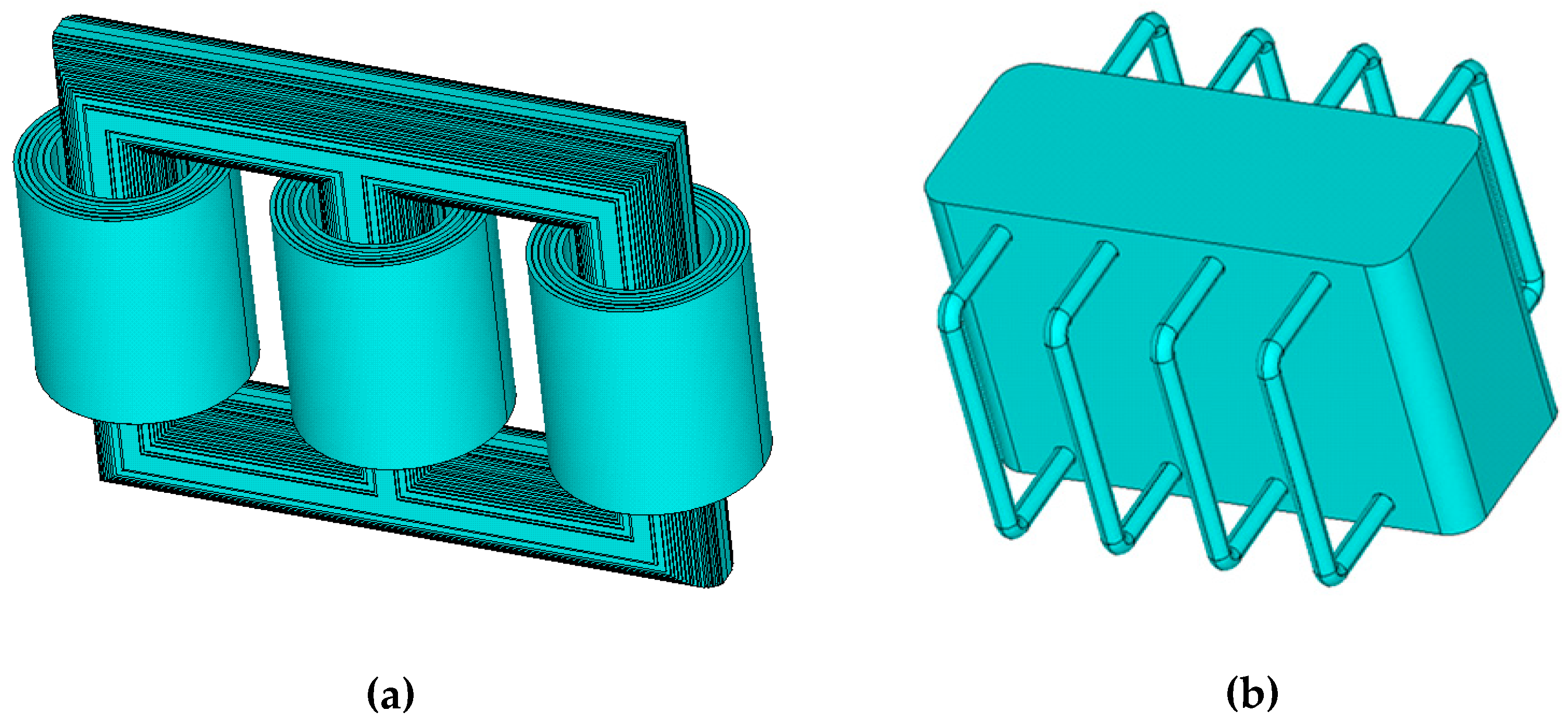
Figure 3.
(a) Transient currents of MV windings; (b) Transient currents of HV windings.

Figure 4.
Magnetic flux density distribution of the transformer core.

Figure 5.
(a) Temperature distribution of the total model; (b) Temperature distribution of the core; (c) Temperature distribution of the LV windings; (d) Temperature distribution of the inner MV windings; (e) Temperature distribution of the outer MV windings; (f) Temperature distribution of the inner HV windings; (g) Temperature distribution of the middle HV windings. (h) Temperature distribution of the outer HV windings.

Figure 6.
Velocity distribution inside three-phase three-limb transformer.


Table 1.
Physical parameters of the transformer oil.
| Parameters of Oil | Function Fitting |
|---|---|
| Density | 1098.72 − 0.712 T |
| Specific heat capacity | 807.163 + 3.58T |
| Heat conductivity | 0.1509 − 7.101 × 10⁻⁵ T |
| Viscosity | 0.08467 − 4 × 10⁻⁴ T + 5 × 10⁻⁷ T2 |
Table 2.
Basic data of 220 kV oil-immersed three-phase three-limb transformer.
| Classification | Value |
|---|---|
| Rated Power/MVA | 180 |
| Rated Voltage/kV | 220/110/35 |
| Frequency/Hz | 50 |
| Connection Group | YNyn0d11 |
| Core type | Planar laminated core |
| Core Weight/kg | 68140 |
| Cooling Type | ONAN |
© 2017 by the authors. Licensee MDPI, Basel, Switzerland. This article is an open access article distributed under the terms and conditions of the Creative Commons Attribution (CC BY) license (http://creativecommons.org/licenses/by/4.0/).
Share and Cite
MDPI and ACS Style
Gong, R.; Ruan, J.; Chen, J.; Quan, Y.; Wang, J.; Jin, S. A 3-D Coupled Magneto-Fluid-Thermal Analysis of a 220 kV Three-Phase Three-Limb Transformer under DC Bias. Energies 2017, 10, 422. https://doi.org/10.3390/en10040422
AMA Style
Gong R, Ruan J, Chen J, Quan Y, Wang J, Jin S. A 3-D Coupled Magneto-Fluid-Thermal Analysis of a 220 kV Three-Phase Three-Limb Transformer under DC Bias. Energies. 2017; 10(4):422. https://doi.org/10.3390/en10040422
Chicago/Turabian StyleGong, Ruohan, Jiangjun Ruan, Jingzhou Chen, Yu Quan, Jian Wang, and Shuo Jin. 2017. "A 3-D Coupled Magneto-Fluid-Thermal Analysis of a 220 kV Three-Phase Three-Limb Transformer under DC Bias" Energies 10, no. 4: 422. https://doi.org/10.3390/en10040422
Note that from the first issue of 2016, this journal uses article numbers instead of page numbers. See further details here.