Article

Near Wellbore Hydraulic Fracture Propagation from Perforations in Tight Rocks: The Roles of Fracturing Fluid Viscosity and Injection Rate

by
Seyed Hassan Fallahzadeh
1,*,
Md Mofazzal Hossain
1,
Ashton James Cornwell
1 and
Vamegh Rasouli
2
1
Petroleum Engineering Department, Curtin University, Perth, WA 6151, Australia
2
Petroleum Engineering Department, University of North Dakota, Grand Forks, ND 58202-6116, USA
*
Author to whom correspondence should be addressed.
Energies 2017, 10(3), 359; https://doi.org/10.3390/en10030359
Submission received: 22 November 2016 / Revised: 6 March 2017 / Accepted: 7 March 2017 / Published: 14 March 2017

Abstract

:
Hydraulic fracture initiation and near wellbore propagation is governed by complex failure mechanisms, especially in cased perforated wellbores. Various parameters affect such mechanisms, including fracturing fluid viscosity and injection rate. In this study, three different fracturing fluids with viscosities ranging from 20 to 600 Pa.s were used to investigate the effects of varying fracturing fluid viscosities and fluid injection rates on the fracturing mechanisms. Hydraulic fracturing tests were conducted in cased perforated boreholes made in tight 150 mm synthetic cubic samples. A true tri-axial stress cell was used to simulate real far field stress conditions. In addition, dimensional analyses were performed to correspond the results of lab experiments to field-scale operations. The results indicated that by increasing the fracturing fluid viscosity and injection rate, the fracturing energy increased, and consequently, higher fracturing pressures were observed. However, when the fracturing energy was transferred to a borehole at a faster rate, the fracture initiation angle also increased. This resulted in more curved fracture planes. Accordingly, a new parameter, called fracturing power, was introduced to relate fracture geometry to fluid viscosity and injection rate. Furthermore, it was observed that the presence of casing in the wellbore impacted the stress distribution around the casing in such a way that the fracture propagation deviated from the wellbore vicinity.

1. Introduction

Hydraulic fracturing is commonly used as the most viable stimulation technique to improve the production rate and recovery factor of oil and gas reservoirs, especially in unconventional reservoirs. When performing a hydraulic fracturing operation in a cased perforated wellbore many problems may arise. These problems lead to high frictional pressure losses near the wellbore, and consequently, would result in significant increase in the operation pressures and eventually premature screen-out [1,2,3]. Additionally, other issues such as multiple fracturing and near wellbore fracture tortuosity have been encountered during the implication of the hydraulic fracturing operation in cased perforated completions [4]. The quality of a hydraulic fracturing operation could be negatively impacted by these issues, and consequently, the fracturing treatment may not improve the production of the wellbore effectively. Such kind of challenges are mainly due to the existence of the perforations cavities which complicate the fracture initiation and near wellbore propagation [5,6].
Several researchers have conducted studies in order to investigate the mechanism of a hydraulic fracture creation in cased perforated wellbores [7,8,9,10,11,12]. They have shown that the wellbore inclination and azimuth as well as perforations spacing, phasing and orientations with respect to the in-situ stress directions play important roles in the process of fracture initiation and near wellbore propagation. Berhmann and Elbel [5] performed an experimental study and showed that when the perforation orientation is deviated more than 10° away from the direction of Preferred Fracture Plane (PFP), the fracture may not initiate from the perforation cavity. Later on, Romero et al. [13] developed a theoretical and numerical model and recognized when the orientation of the perforation gun is not properly designated, it could lead to a narrow fracture. Accordingly, the fracture width close to the wellbore wall would be narrower than the width of the main body of the fracture. This has been later investigated further through an analytical study. Fallahzadeh, et al. [11] found that when the perforation direction is oriented away from the direction of the tensile zone on the wellbore circumference, the fracture initiation pressure also increases.
Additionally, several experimental studies have been carried out in order to physically model and analyze the mechanism of fracture creation in perforated boreholes [5,6,14]. However they did not scaled down the real field fracturing processes to experimental test samples. These sets of experimental research could had been greatly improved by the application of proper scaling analysis. Van de Ketterij and de Pater [15,16], developed and implemented the scaling laws in their fracturing experiments. They investigated the effects of fluid viscosity and injection rate on fracturing pressure; nevertheless, but they only modeled a deviated wellbore with an azimuth of 60° and an inclination angle of 49° and did not comprehensively analyze the effects of these two parameters on fracture geometry.
Therefore, this experimental study was performed to systematically examine the effects of fracturing fluid viscosity and injection rate on the fracture initiation and break down pressures and also near wellbore propagation geometry. Synthetic low-permeable mortar samples with specific properties were made for the purpose of performing scaled hydraulic fracturing tests. Scaling analyses were conducted, and a true tri-axial stress cell (TTSC) was used to simulate the three in-situ principal stresses on 150 mm synthetic cubic samples. Three high viscous fluids were used as the fracturing fluid. These fluids included honey, and two different silicone oils. The fracturing fluids were used to conduct scaled hydraulic fracture experiments on nine synthetic samples. For each sample, a particular fluid was injected with a specific flow rate ranging from 0.05 to 5 cc/min. The fracturing fluid was injected through the casing and two perforations located at the center of the sample.
To properly analyze the tests’ results, a new methodology is developed for predicting the fracture propagation time from the pressure-time curves. Accordingly, the fracture initiation and break down pressures are analyzed based on the particular fluid viscosity and injection flow rate applied for each test. Two new parameters, namely fracturing energy and fracturing power, are introduced in order to improve the interpretation of the results. Subsequently, the near wellbore fracture propagation geometry is characterized by the initiation angle it makes at the perforation tunnel, and the propagation path it grows in. The geometries of fractures are then compared against the fracturing energies and powers of the corresponding tests. Consequently, a new relationship is introduced to estimate the fracture initiation angle from the fracturing power. Moreover, some effects of the casing and its surrounding cement sheath properties on the fracturing process are discussed.

2. Sample Preparation

In this section, the process of sample preparation is discussed. This process includes preparing appropriate cement and sand slurry mix and casting the slurry in cubic moulds. Then cased wellbore and perforations are created in the samples after casting and curing were completed. At the end of this section, the properties of the synthetic sample and fracturing fluids are presented.

2.1. Casting Cement Samples

To conduct scaled hydraulic fracturing tests, rock samples with particular hydro-mechanical properties are required. However, rock samples with desired properties are not readily available as it is practically impossible to acquire a sufficiently large size intact sample from a wellbore. Additionally, the properties of rocks obtained from an outcrop (considering that they are a good representative of downhole rock samples) may not be homogeneous. Also, outcrop rock samples are typically very porous and permeable. Such rocks would have considerable fracturing fluid leak-off if subjected to experimental hydraulic fracturing tests. Since the experiments have relatively low injection rate, most of the fluid would be leaked off, as a result, no fracture would be formed. Therefore, synthetic mortar samples were made to conduct these laboratory experiments, because it is possible to prepare these samples with reasonably homogenous properties [17].
The components of synthetic samples are cement, sand and water. Mechanical and hydraulic properties of any synthetic sample are significantly affected by the percentage of each individual component used in the cement slurry preparation. During sample preparation, it was observed that a slight variation in the ratio of the components of the cement slurry could significantly alter the characteristics of the final concrete block. This emphasizes the importance of systematic selection of the cement, water and sand ratios.
The synthetic samples prepared in this study were produced based on the procedure presented by [18]. The proposed cement slurry mixture consisted of Portland cement-sand and water-cement weight ratios of 1 and 0.4, respectively. Initially, dry sand and cement were adequately mixed and then water was added to the mixture. The cement, sand and water were gradually mixed together using a heavy duty mixing equipment in a way that it reduced the volume of the air bubbles entering the slurry whilst also producing a homogenous mixture. The optimum mixing time was found to be 15 min at which point a uniform grain distribution was achieved.
In addition, the sand grain size distribution influences the sample properties. Therefore, sand grain sizes were carefully chosen to be in the range of 200 μm to 850 μm in order to have a low permeable final mortar block. Figure 1 shows the grain size distribution used to prepare the samples. A Low permeable sample is a good representative of tight formations in unconventional reservoirs. Also, it reduces fracturing fluid leak-off, which is suitable for scaling analysis. This is explained in more details in Section 4.
To simulate the real field in-situ stress conditions, the experiments were planned to be carried out on cube-shaped samples, where three independent stresses could be applied. Therefore, standard concrete cubic moulds were used to make 150 mm × 150 mm × 150 mm mortar blocks. The cement slurry was poured into the cubic moulds which were slightly overfilled to compensate for the slight shrinkage of the cement. After filling the moulds the samples were placed on a vibration plate so that the air bubbles present within the slurry moved their way to the surface. It was found that the optimum vibration time was around 10 minutes. This was a sufficient amount of time for air bubbles to graduate from the slurry with no separation of particles within the mixture due to its relatively high viscosity. Finally, around an hour after the casting, in which time the cement samples had partially shrunk, the top side of the samples were flattened using a wet trowel. The samples were then allowed to set for a day after which time they were removed from their moulds and placed in a water bath for 28 days. This allowed the cement to cure and reach its ultimate compressive strength [19].

2.2. Preparing Cased Perforated Samples

In the next step, a wellbore had to be drilled into each sample with its entire length being cased. This is mainly because the existence of the casing could significantly affect the wellbore stress distribution, and consequently, the fracturing pressure and near wellbore fracture geometry would be affected [20]. Stainless steel tubing with an outer diameter of 12.7 mm, that could withstand a maximum internal pressure of 48.3 MPa, was selected to be used as the casing.
A wellbore was drilled directly through the center of each sample. The hole was drilled at 650 rpm through the entire length of the sample with a 14 mm masonry drill bit. The slow rate of penetration ensured maximum cutting efficiency. The hole was drilled as soon as the sample was removed from the water bath to reduce the risk of micro cracks forming around the wellbore.
The hole was then cleaned and a 400 mm long piece of the aforementioned tubing was cut to be glued in the wellbore. A part of the tubing (150 mm) was accommodated in the wellbore and the rest of the tubing was considered for connection purposes to the fracturing fluid chamber. This will be explained in more details in Section 3.2. As the OD of the tubing was 12.7 mm and the wellbore diameter was 14 mm, a narrow annulus of only 0.65 mm wide was considered for the placement of adhesive. Such narrow annulus was designed to minimize the effect of the adhesive on casing and wellbore stress distribution, for the time when the cubic sample would be under stress. However, some difficulties arose due to this narrow annulus, when gluing the tubing in the hole. The adhesive material was quite viscous and it could not easily fill and seal the annulus between the casing and the wellbore. To resolve this problem, initially the tubing was plugged at one end by an 8 mm OD steel rod. Then it was slightly roughened to provide a better bond between the casing, glue and block. Next, one side of the wellbore was placed on a rubber sheet and enough adhesive was carefully poured into the wellbore from the other side. At this stage, the plugged end of the tubing was inserted into the wellbore and firmly pushed against the adhesive at the bottom of the hole. While enough force was applied and the rubber sheet was sealing the bottom side of the wellbore, the adhesive flowed upward in the annulus and filled the whole space. This upward flow of the adhesive ensured that no air bubble was left in the narrow annulus and consequently guaranteed the sealing of the dried adhesive.
It is noteworthy that the first tubing was glued in the wellbore using Selleys Liquid Nails adhesive. However, the rest of the samples were prepared using Super Strength Araldite adhesive. This was mainly because the former glue did not demonstrate enough strength and the fracturing fluid could break through it, when the fracturing test was in progress. This is discussed in more details in Section 5.2. The strength properties of these adhesives are presented in Table 1.
The wellbore glue was allowed to cure for three days at which point two perforations were drilled into each sample. Each one was drilled at the center of two parallel faces of a sample, perpendicular to the wellbore so that the perforations were facing directly opposite each other. The perforations were drilled through to the casing with a 4 mm masonry bit and a 4 mm general purpose drill bit through the steel casing. Each perforation was then cleaned and plugged with 35 mm of 3.75 mm steel rod using Araldite. The samples were allowed to cure for another 3 days. After that, they were cleaned up using a variety of files and sandpapers to guarantee that each surface of the sample was completely level. This would ensure a uniform stress distribution being applied to each face when under stress. Then the samples were left in ambient conditions for 30 days to dry before the tests.
Before each sample was placed inside the TTSC, a steel rod 380 mm in length and 6.2 mm in OD was placed in the wellbore to minimize the volume of the wellbore. Hence reducing the wellbore filling time once the test would commence. The other benefit of having this rod was to reduce the dead volume of the fracturing fluid. As a result, when the fracturing test was in progress, less compressed fracturing fluid would be present inside the hole at the time of fracture break down. Therefore, the fracture propagation could be better controlled.
The completed samples were then representative of a cased and perforated wellbore. The perforations were aligned perpendicular to the minimum horizontal stress in the TTSC in order to promote fracture initiation. Figure 2 shows a schematic of the cased perforated block.
To perform scaling analysis for hydraulic fracturing experiments, samples’ physical and mechanical properties as well as fracturing fluids’ viscosity are required. Table 1 presents a summary of the physical and mechanical properties of the samples as well as the adhesives’ strength properties.

3. Experimental Set-Up

3.1. True Tri-Axial Stress Cell (TTSC)

For conducting the fracturing tests three independent stresses should be applied on each cubic sample to simulate the underground in-situ stresses. To achieve this objective, a true tri-axial stress cell (TTSC) was implemented [21]. The TTSC is capable of applying three independent orthogonal stresses in three directions on a sample. These stresses are applied to a sample using a series of hydraulic rams which are powered by three separate syringe pumps.
Each syringe pump can provide up to a maximum pressure of 9500 psi, and a maximum injection rate of 107 cc/min. The TTSC is designed in such a way that it could accommodate cubic samples of up to 300 mm in size. However, with the aid of a number of aluminum spacer blocks the TTSC could also be employed for testing a variety of smaller cubic sized samples. In this particular study, six 145 mm× 145 mm × 75 mm spacers were applied to properly accommodate the prepared samples at the center of the TTSC. The face of each spacer, which comes into contact with the face of the sample is 5 mm smaller on each side. This would ensure that the adjacent spacers would not come into contact with each other when there is some displacement of the sample. Figure 3 shows a top view of the TTSC and the syringe pumps, which were used for applying the stresses, and also a 150 mm sample accommodated in the cell using the spacer blocks.
As it was mentioned in the introduction section, the main goal of this study was to investigate the effects of the fracturing fluid viscosity and flow rate on the fracture initiation and near wellbore propagation geometry. Therefore, a particular stress regime was considered to be applied on all samples in this study. This would have ensured that the stress regime would not influence the tests’ results. Consequently, a maximum principal stress (σ1) of 13.8 MPa (2000 psi), an intermediate principal stress (σ2) of 10.3 MPa (1500 psi), and a minimum principal stress (σ3) of 6.9 MPa (1000 psi) were applied on each sample. Such stress components would represent a normal in-situ stress regime where σ1 > σ2 > σ3. It is noteworthy that no scaling was considered for the applied stresses; however, scaling analyses were performed involving the energy dissipation during fracture growth (see Section 4).
In ideal circumstances, it is expected that a hydraulic fracture initiates and propagates in a plane known as preferred fracture plane (PFP), which is perpendicular to the minimum principal stress direction. Therefore, all testing samples were placed in the cell in such a way that the perforations were along the direction of the intermediate principal stress. Also, the maximum principal stress was set along the wellbore axis. This would facilitate and ease the fracture to be developed in PFP.
It is noteworthy that the principal stresses were applied in three stages. Initially, all three stresses were concurrently increased to the minimum principal stress magnitude. At this point, the corresponding minimum stress syringe pump was set on a constant pressure mode to simulate the minimum in-situ stress perpendicular to the direction of the perforations. Then the other two stresses were increased to the intermediate principal stress, and at this stage, the intermediate stress was kept constant. At the final stage, the maximum principal stress was increased to its required value and then its corresponding pump was set on constant pressure mode. This stress path was consistently applied to all samples tested in this study.

3.2. Fracturing Fluid Injection

Three high viscous fluids were used as the fracturing fluid to examine the effects of viscosity on fracturing pressures and propagation geometry. These fluids included honey, and two different silicone oils. The properties of these fluids are listed in Table 2. The fracturing fluids were used to hydraulically fracture nine synthetic samples, and for each sample a particular fluid was injected with a specific flow rate ranging from 0.05 cc/min to 5 cc/min. Viscosity of silicone oils used in this study is obtained from manufacturer database, which is assumed to be reliable. It is also assumed that behaviour of these fluids was Newtonian. This is due to the fact that the fracturing tests were conducted with very low injection rate for which the shear rate of these fluids are observed to be well below its critical shear rate. Therefore, it is reasonable to consider the behaviour of these fluids was Newtonian for these tests.
A displacement chamber with a total volume of 120 cc was used along with a syringe pump to inject the high viscous fracturing fluid into the wellbore. The chamber was carefully cleaned and filled with the desired fracturing fluid before each set of tests. This process was strictly followed to make sure that no air bubbles could enter the fluid. Since air bubbles can easily get trapped in the high viscous fracturing fluids resulting in a detrimental effect on the fracturing experiment. This is due to the fact that air is much more compressible than the fracturing fluid. Therefore, when the wellbore is being pressurized with the fracturing fluid, the air bubbles shrink, while maintaining the same pressure as the wellbore. Once the fracture initiates in the sample, some new volume would be created and as a result some wellbore pressure reduction is expected. This variation in the wellbore pressure will be interpreted later to analyse the fracturing pressures and geometries. However, with the presence of compressed air bubbles, they could easily expand and compensate for the newly created volume. Consequently, the wellbore pressure would not reduce much and the fracturing process may be misinterpreted. In addition, the expansion of the air bubbles could provide sufficient pressure to propagate the fracture very quickly to the boundary of the sample (i.e., uncontrolled fracture propagation), which is not favorable.
As three different fracturing fluids were used for these experiments, testing required the fluid chamber to be filled with the three different fluids. The nature of these fluids, particularly their high viscosity made this filling process to become a cumbersome and time-consuming task. An alternative and more efficient approach was to first fill a larger chamber with a capacity of 750 cc, then allow the viscous fluid to settle in the chamber. And finally pressurising the chamber and slowly releasing the pressure so that all the air bubbles were removed from the fluid. The fracturing fluid was then displaced into the smaller fluid chamber before testing took place.
In order to inject the fracturing fluid into the wellbore, the fluid chamber should have been connected to the tubing of the sample. As it is seen in Figure 3, there is a hole at the bottom of the cell which is designed for the sample’s casing to pass through. The top side of the casing, (located underneath the cell), is at the point where the fracturing fluid chamber was connected. Once testing commenced, the fracturing fluid was injected into the borehole of the sample from beneath the TTSC. Two pressure transducers, called pre and post choke transducers, were used to measure the injection pressure. These transducers were installed as close to the sample as possible and separated by a partially opened needle valve which acted as a choke (flow restrictor). Figure 4 shows a schematic of the fracturing fluid injection set-up. It should be noted that each synthetic sample was initially accommodated in the TTSC (Figure 3) and then it was connected to the fracturing fluid injection line.
The choke helped to restrict and regulate the flow of the fracturing fluid which enabled more precise controlling of fracture growth [23]. Considering the moment at which the wellbore is pressurized enough so that a fracture initiates from the perforation(s), some new volume is expected to develop. This leads to a reduction in wellbore pressure. Therefore, the pressurized fluid, which is in the fracturing fluid chamber, would naturally flow at a higher flow rate towards the wellbore to compensate for this pressure reduction. This would consequently provide higher pressure in the wellbore and the initiated fracture would propagate uncontrollably and quickly towards the boundary of the sample. Such fast fracture growth in the laboratory-scale could not be reasonably compared with field-scale fracture propagation. Hence, the choke could control the flow of compressed fracturing fluid into a newly initiated fracture and accordingly would control the fracture propagation speed.

4. Scaling Analysis

In order to reasonably compare the results of laboratory scale hydraulic fracturing experiments to field scale operations, it is fundamentally important that scaling laws are applied. Scaling laws are simply the dimensional analysis involving the energy dissipation during fracture growth. Known information such as sample size, wellbore dimensions and the hydro-mechanical properties of the sample are normally used as the inputs into the scaling model. This enables the output variables such as fluid viscosity, injection rate and total fracture propagation time to be properly calculated and aided in the design of the laboratory hydraulic fracturing test [24].
At the laboratory scale, some of previous experimental works were conducted without the consideration of scaling laws [25]. As a consequence, experimental parameters such as fluid viscosity and injection rates were based on the values used in real field operations. This resulted in very low fluid viscosities and highly exaggerated injection rates being used in the laboratory. However, in order to properly monitor and analyze the fracture initiation and propagation in a small sample at lab scale, fracturing fluids with significantly higher viscosities are often required as well as drastically reduced injection rates. This ensures that the fracture is contained within the sample and allows fracture growth to be monitored without being affected by boundary conditions.
During hydraulic fracturing, the time at which the wellbore pressurization rate reaches its maximum value is recognized as the fracture initiation point. Therefore, in this study, the fracture initiation time was considered as the reference point for scaled time. Conversely, fracture breakdown is usually defined as the time at which the wellbore pressure reaches its maximum value, and fracture initiation typically occurs before this breakdown point [26]. Therefore, the scaling period of a laboratory experiment starts with fracture initiation and runs through to the final stage of the fracture propagation.
Over the course of a hydraulic fracturing operation in the field, the initiation and propagation of the real fracture is influenced by three essential boundaries of viscosity, toughness and leak-off dominated regimes [23]. In these tests, the permeability of the samples was around 0.019 mD and therefore the effect of leak-off and the leak-off regime could be regarded as negligible. During the majority of field fracturing operations, fracture growth is predominately toughness dominated throughout fracture initiation. However, as the fracture develops it rapidly becomes viscous dominated [27]. Furthermore, for a radial fracture, the regime becomes more toughness dominated during the final stage of the fracture growth [28]. In this study scaling laws developed by de Pater et al. [24] were applied. Also the scaling analysis developed in a recent study [23,26,28] was used to ensure that the majority of the fracture growth is viscous dominated similar to what happens in a field fracturing. In order to have viscous dominated fracture propagation the following equation should be satisfied [24]:
K I C < 2 P n r f π
Here, KIC is the fracture toughness, Pn is net fracture pressure and rf is fracture radius. Considering the hydro-mechanical properties and dimensions of the samples used in this study, the right hand side of Equation (1) is always larger than the synthetic sample’s fracture toughness. This is valid for the range of injection rates and fluid viscosities considered for this study. However, the injection time is different for each set of fracturing fluid viscosity and flow rate; this is more explained in Section 5.1.
In order to have a viscous dominated propagation regime, the dimensionless toughness parameter of a Penny-Shaped fracture can be calculated using the following equation [28]:
κ = K ( t 2 μ 5 Q o 3 E 13 ) 1 18
In this equation, t is the time of experiment and Qo′ is flow rate. In theory, based on Equation (2), the fracture propagation will be viscous dominated if κ is less than one, whereas if κ is greater than four the propagation will be toughness dominated [28]. It must be noted that the dimensionless toughness number, κ is time dependent; hence the fracture regime may change as time evolves. Other parameters are as follows:
K = ( 32 π ) 1 2 K I C
E = E 1 ν 2
μ = 12 μ
where, μ is fracturing fluid viscosity, E is rock’s Young’s modulus, and v is the Poisson’s ratio. Using the samples’ hydro-mechanical properties (Table 1), fracturing fluid viscosities (Table 2), and the range of the flow rates, which were used in this study, the dimensionless toughness numbers (κ) as presented in Equation (2) were calculated and presented in Table 3. The other parameters in Equation (2) are calculated using Equations (3)–(5). As it is seen in this table, all κ values are less than one, confirming that the conducted experiments in this study would have viscous dominated fracture propagation.
It is noteworthy that the time of the experiment is 1000 s, which was selected based on the previous experimental experiences. Also, it was observed that in all of the experiments, the propagation time was less than 1000 s. This would result in a κ value smaller than one, as κ is directly proportional to the propagation time.
It should also be mentioned that while the scaling laws are used in this study, the non-homogeneous nature of the samples may negatively impact the results. This may cause a difficulty in extrapolating the results to large scales. Generally, it is not practically possible to scale micro-structural properties like the ratio of the fracture length to grain size in laboratory and field operation [24]. Therefore, in this study, the effect of grain size on fracture initiation and propagation is ignored.

5. Results and Discussion

During this investigation, hydraulic fracturing tests were conducted on nine 150 mm cubic concrete samples. The tests involved the use of three different fracturing fluids and a range of injection rates from 0.05 cc/min to 5 cc/min. The samples were prepared with significant level of caution and care to ensure that the stress distribution being applied to each face of the sample was uniform. Further to this, the wellbore and perforations were prepared with repeatability to make sure that the stress distribution applied by the high-pressure fracturing fluid would be near identical in each sample.
This allowed the control of the majority of the variables present in the experiment, and the accurate monitoring and study of the effects of varying the fracturing fluid viscosity and fluid injection rate. A normal stress regime was maintained throughout the testing on all nine samples, where σ1 = 13.8 MPa, σ2 = 10.3 MPa, and σ3 = 6.9 MPa. Table 4 presents the fracturing tests’ parameters and the fracture initiation and break down pressures for each test.
As previously mentioned, two pressure transducers were used to record the pre (P1) and post (P2) choke pressures, just at the entrance of the wellbore (see Figure 4), while the fracturing fluid was being injected into the wellbore. Due to the fact that the length of the wellbore was relatively short and the injection rates were quite low, the frictional pressure drop was negligible. Table 3 presents the maximum frictional pressure loss for each fracturing fluid at its maximum injection rate. Since the frictional pressure loss was negligible, the post choke pressure reading could be considered as the fracturing pressure (i.e., the wellbore pressure). However, the pre choke pressure reading was used as a means to estimate the initiation and breakdown pressures. Figure 5 shows a pressure-time curve corresponding to test SL-1. In this figure, the pre and post choke pressures (P1 and P2) are shown as well as the wellbore pressurization rate. In addition, the difference between P1 and P2 is calculated and displayed versus time. This would greatly help in predicting the moment of fracture initiation as well as predicting the fracture propagation time.
As it is seen in Figure 5, over the first 550 s of the injection time, the pressure recording did not increase much. In this time the fracturing fluid was just filling the wellbore and the perforations. After the wellbore was completely filled, the two pressures started to build up and as a result, the wellbore was pressurized.
The initiation pressure could be estimated as the point where the pre and post choke pressure readings begin to deviate from each other, whereas the breakdown pressure is taken as the maximum wellbore pressure. In essence, as the wellbore is being pressurized, both the pre and post choke pressures would be increasing. However, when the fracture initiates, micro fractures are created and hence the rate of increase of the wellbore pressure reduces. This is due to the fact that the pressurized fracturing fluid in the wellbore expands to fill the volume of the newly initiated flaws and consequently the wellbore pressure decreases. However, because of the presence of the choke, the pre choke transducer does not sense this reduction in pressure and increases more than that of post choke pressure. Therefore, the point at which the difference between the two pressures increases indicates the fracture initiation (see Figure 5).
The other evidence to mark the fracture initiation point is the reduction in the wellbore pressurization rate. This is basically due to the fact that as a fracture initiates, the wellbore pressure reduces and consequently the pressurization rate would decrease. This reduction in the pressurization rate along with the increase in the difference between the pre and post choke pressures were implemented in all these tests to precisely specify the moment of fracture initiation.
At the conclusion of each test, the in-situ stresses were reduced at a constant rate back down to atmospheric pressure. The sample was then taken out of the TTSC, at which point it was carefully broken apart along the induced fracture planes. The fracture planes were then photographed to aid analyzing the fracture geometries. Also, the pressure-time curves were used to interpret the initiation and breakdown pressures, as well as near wellbore fracture geometry. Table 5 presents a brief description of the fracture geometries.

5.1. Predicting Fracture Propagation Time

In laboratory fracturing experiments, fracture propagation time is generally considered as the time interval it takes for an initiated fracture to grow from the wellbore (or the perforations) all the way to the boundary of the experimental sample. This time interval is critically important in such experimental studies. This is because when the fracture propagates and the fracture tip gets close to the boundary of the sample, the last moments of fracture propagation may be influenced by the sample’s boundary conditions. Therefore, the very last stages of the fracturing process may not appropriately represent the real field fracturing mechanism. In addition, any further injection of the fracturing fluid after the fracture has reached the boundary may resemble real hydraulic fracture propagation and mislead the experiment’s interpretations.
Such issue is marked and shown in Figure 5, where after the fracture reached the sample boundary, the rest of the pressure recording data was just showing the fracturing fluid flowing through the created fracture all the way to the boundary of the sample. It should be noted that such pressure behavior is very similar to hydraulic fracture propagation in the field, where the wellbore pressure remains almost constant. Therefore, it is critically important to consider a methodology in order to properly detect the end of the fracture propagation and disregard the rest of the pressure curve.
As it is explained in Section 4, the fracture propagation time (injection time) could be obtained using theoretical scaling analysis. The scaling analysis is based on some assumptions such as a penny-shaped fracture propagation. All these assumptions may not be valid in a case where a real hydraulic fracturing test is in progress. Therefore, the estimated required injection time may not match the real one. For instance, when a fracture is initiated from a perforation and it is propagated along a curved path, due to the concentrated stress distribution around the wellbore and the perforation, it is not actually a penny-shaped fracture. Therefore, as it is contradicting the assumptions of the scaling laws, such curved fracture propagation may not be accurately matched with scaling analysis.
In order to address this problem, a new methodology was developed in this study to interpret the fracturing pressures. In this methodology real propagation time (or its corresponding injection time) could be directly estimated from the pressure recordings. This methodology is based on the concept of fluid flow through a fracture. When a fluid with a constant viscosity and under isothermal conditions is flowing through a constant length fracture, the frictional pressure loss along the fracture would not change over time. When the fracture tip reaches the boundary of the sample, the length of the fracture does not increase any more. Accordingly, the rest of the wellbore pressure curve would present an almost constant pressure behavior versus time. This means that the wellbore pressurization rate would become almost zero.
Conversely, one stage earlier, when the fracture initiates and propagates through the sample, as the tip of the fracture is growing, it creates new volume. Consequently, the fracturing fluid would expand to fill this volume, and as a result, the wellbore pressure would decrease. However, this pressure reduction pulse would take a short while to pass across the fluid restrictor (the choke); therefore, the pre choke pressure (P1) may not decrease simultaneously. Accordingly, the pressure difference (ΔP = P1 − P2) would increase (see Figure 5). However, after a short while, the pre choke pressure would also decrease as a result of sensing the pressure pulse, and would accordingly support the wellbore pressure. Nevertheless, as the fracture is growing, more and more volume would be generated and the wellbore pressure keeps decreasing, especially after the fracture breaks down. This is indicated in Figure 5, where the wellbore pressurization rate is decreasing after the fracture break down point; simultaneously, the difference between the two pressures (ΔP) is still increasing.
Once some fracture length is created, the rate of fracture propagation would stabilize. This is because the tip of the fracture is moving far from the wellbore and perforation stressed zone. Therefore, it is approaching a less stressed region (concurrently, the wellbore pressure is now less than break down pressure, therefore less pressure is provided in the fracture for the purpose of its propagation). As a result, the wellbore pressure would decrease less and this means that the pressurization rate would approach zero. Similarly, ΔP would firstly stabilize and then decrease.
As the fracture tip hits the boundary of the sample, the fluid can flow out of the sample. This means that the wellbore pressure is now equal to the fracturing fluid frictional pressure loss along the created fracture. Because this pressure loss does not change over time, the wellbore pressure would stabilize. This is the point where the pressurization rate becomes zero and ΔP would also stabilize. This point could practically be considered as the end of the fracture propagation, and the rest of the pressure-time data would represent the fluid flowing in the fracture (see Figure 5). This methodology has been implemented for all the tests in this study, and the fracture propagation of every test is presented in Table 4.
To illustrate the fracture propagation time, tests H-2 and H-3 could be compared. As it is presented in Table 4, honey was used as the fracturing fluid to conduct these two experiments. Test H-2 was initially intended to be fractured under a flow rate of 1 cc/min. However, after 3100 s of injection, no fracture was initiated (based on the pressure-time curve). Therefore, the flow rate was then increased to 2 cc/min. Test H-3 was also performed using a flow rate of 2 cc/min; however, the pressurization time of this test was 900 s only. This might be the main reason of the difference between the fracturing pressures of these two tests. Nevertheless, when the corresponding fracturing pressure curves were analyzed using the aforementioned method, it was detected that the fracture propagation time of test H-2 was 320 s, while the other test had a fracture propagation time of 669 s.
Referring to Figure 6, where the fracture geometries of these two tests are shown, it is seen that in test H-2 a planar fracture was propagated, and the fracture tip reached the side boundary of the sample before the fracture has propagated much in the vertical direction. This has resulted in a relatively small propagation time and consequently a small fracture plane. While test H-3 experienced a curved fracture geometry which turned away from the wellbore and aligned itself almost with PFP before the tip of the fracture reached the top boundary of the sample. As a result, a larger fracture plane was created in test H-3 in comparison to that of test H-2 and this confirms the longer fracture propagation time in test H-3, as it was predicted from its pressure-time curve.

5.2. Cement Sheath Strength Effect

A common practice in the completion of an oil or gas wellbore is to cement the production casing in the open wellbore across the pay zone. This is achieved by pumping cement slurry with some particular rheological properties down the hole and then the slurry would flow upwards in the annulus between the casing and the wellbore wall. Eventually, the drilling engineers will wait for a fraction of a day or a few days for the cement to set, before they move on to the next operation [29]. From the drilling engineer point of view, the set cement should support the weight of the casing and for this reason, it should reach a minimum strength of 34.5 MPa (5000 psi) [30]. This would be equivalent to a tensile strength of 3.4 MPa.
Such low strength properties might be sufficient to support the weight of the casing for wellbore drilling purposes. However, later on over the life of the wellbore, if the production engineer hydraulically pressurizes the wellbore and perforations, the fracturing fluid may propagate a fracture through the cement sheath rather than the formation rock. This is what was observed in the first test, where the pressurized fracturing fluid created multiple fractures through the solid adhesive (which was essentially used as the cement slurry to bond the casing to wellbore wall). Consequently, no fracture was developed in the sample.
Figure 7 shows the fracturing pressure curve and a view of the sample in test H-1, which was broken by hammer after the test. As it is demonstrated by the pressure-time behavior, one may conclude that multiple fractures were initiated and propagated in the sample. This is because the curve does not reveal any point that could indicate the failure of the adhesive. However, when the sample was inspected after the test, it was realized that the fracturing fluid had actually created a micro-annulus and had leaked out of the sample just next to the casing. A further analysis, which was done after the sample was split apart using a hammer and a chisel, showed that no fracture was initiated within the sample, though both perforations had been pressurized by the fracturing fluid.
The same issue may happen in a real hydraulic fracturing operation. A pressurized fracturing fluid could break through a low strength cement sheath in the annulus of the wellbore, while its pressure-time graph on the surface may appear to be very similar to a proper hydraulic fracture propagation in the formation. It is noteworthy that, in such condition, where the fracturing fluid has created a fracture in the cement sheath, it is more likely that the fracture would propagate upwards. This is because less stress would be applied to the tip of the fracture at shallower depths. Consequently, this may negatively impact the integrity of the wellbore. Therefore, it is crucial to investigate the cement strength properties before any hydraulic fracturing operation is performed in a cased perforated wellbore.
To prevent this problem in the rest of the samples, they were prepared using Super Strength Araldite adhesive. This was in contrary to sample H-1, which was glued using Selleys Liquid Nails adhesive with a shear strength of 1.1 MPa (see Table 1). The Super Strength Araldite offered a shear strength of 26 MPa, and had appropriately sealed the annulus in the rest of the tests with no instance of a micro-annulus incident.

5.3. The Effects of Viscosity and Flow Rate

According to the scaling analysis presented in Section 4, to conduct a scaled hydraulic fracturing experiment, the use of a very high fracturing fluid viscosity is necessary. This is basically to properly simulate the real physical phenomena taking place over the course of a field hydraulic fracturing process to laboratory experiments [24]. The other important parameter that is involved in the fracturing process is the injection flow rate. Typically, in laboratory experiments, when a very high viscous fluid is used, the injection flow rate should be much lower than the field operation injection rates [25]. In this study, three different fracturing fluids were used, and in each test a particular injection flow rate ranging from 0.05 to 5 cc/min was considered to investigate the impacts of these two important parameters on fracturing pressure, propagation and near wellbore geometry.
Because every test had a specific flow rate and viscosity, the product of flow rate and viscosity (Q × μ) is considered in order to ease the tests’ results comparison and simplify the analysis. Considering the unit of flow rate (m3/s) and the unit of viscosity (N.s/m2), it is realized that the unit of the product of flow rate and viscosity will be N.m. This means that the product is representing the energy which is supplied for hydraulic fracturing. Such fracturing energy concept is later used to better interpret the tests’ results.

5.3.1. Fracturing Pressures

Fracture initiation and break down pressures are the two most critical parameters of a fracturing operation, especially in cased perforated wellbore. Analyzing the fracture initiation and break down pressures presented in Table 4 along with their corresponding fracturing fluid viscosities and flow rates would reveal that as the product of flow rate and viscosity increases, generally higher pressures are experienced.
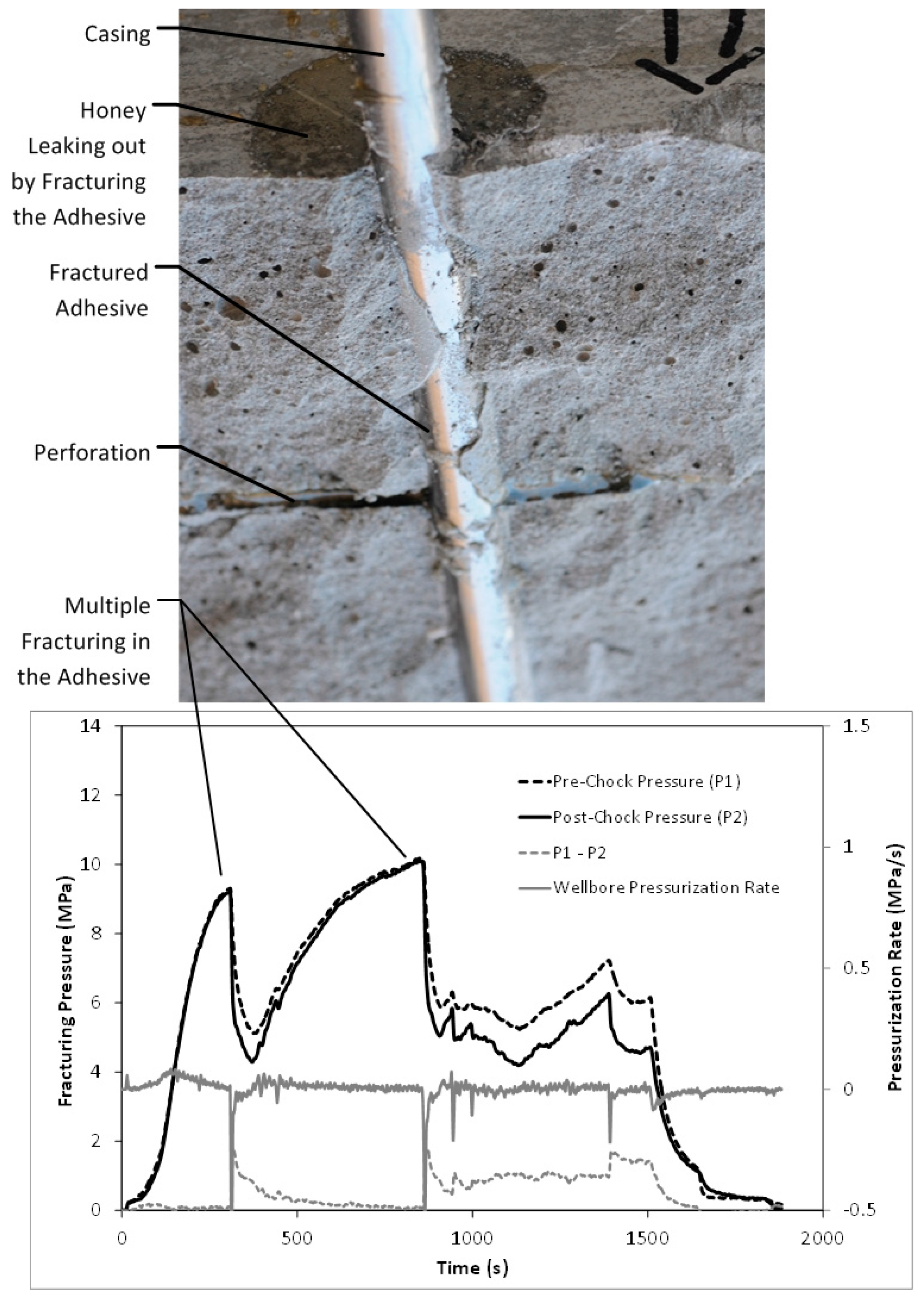
For instance, test SL-3, was performed using silicone oil as the fracturing fluid with a viscosity of 97,700 cp, and the injection flow rate was 0.05 cc/min. This sample exhibited multiple fracturing and the first fracture was initiated at a pressure of 7.98 MPa and its break down pressure was 8.16 MPa. This first fracture did not propagate much and the wellbore pressure increased again and the second fracture was initiated at a wellbore pressure of 14.37 MPa and at this time the break down pressure was recorded to be 14.65 MP. Comparing this test with test SH-1, in which silicone oil viscosity was 586,800 cp and the injection flow rate was 1 cc/min, it is observed that the latter test demonstrated a much larger fracturing pressures. In which the initiation and break down pressures were 32.75 MPa and 35.65 MPa, respectively.
Similarly, comparing tests SH-1 and SH-2 would lead to the same result. These two tests were both conducted using silicone oil with a viscosity of 586,800 cp; however, the injection flow rate in test SH-2 was one tenth of the flow rate in test SH-1. Consequently, in test SH-2, the fracture was initiated at a pressure of 28.27 MPa, while it was 32.75 MPa in test SH-1. The break down pressures also showed a difference of almost 3 MPa between the two tests. These comparisons highlight that a larger product of injection flow rate and viscosity would lead to higher fracturing pressures.
This is mainly because as a viscous fracturing fluid is injected at a higher flow rate, more energy is supplied to the wellbore. Consequently, the wellbore pressurization rate increases. This makes the fracturing process more dynamic, and as a result larger fracture initiation and break down pressures would be required to create a fracture. Physically, when a rock or concrete sample is loaded dynamically, it would exhibit larger strength parameters [31]. The same concept appears to be valid for a hydraulic fracturing test, further research is required to investigate this in more details.

5.3.2. Fracture Geometry

The geometry of the hydraulic fracture (specifically near the wellbore) plays an important role during the fracturing operation. A more planar fracture plane would result in a wider fracture with lesser frictional pressure loss. Additionally, the chance of proppant bridging over a planar fracture plane is lower. Moreover, a planar fracture plane is favorable for hydrocarbon production, because oil and gas could flow through such fracture with less pressure reduction.
A description of fracture geometries for every sample is presented in Table 5. Analyzing these fracture geometries along with the experimental parameters (see Table 4) would demonstrate how the injection flow rate and fluid viscosity may influence the near wellbore fracture geometry. Generally, because every sample had two perforations parallel to the direction of intermediate stress (maximum horizontal stress), it was expected that a two-wing fracture plane would be initiated from the top and bottom side of each perforation. And then it would propagate vertically, perpendicular to the direction of minimum stress. However, most of the fractures were initiated in an angle with respect to the vertical plane (herein preferred fracture plane), and propagated in a curved path away from the wellbore and eventually, the tip of the fractures grew towards the vertical plane.
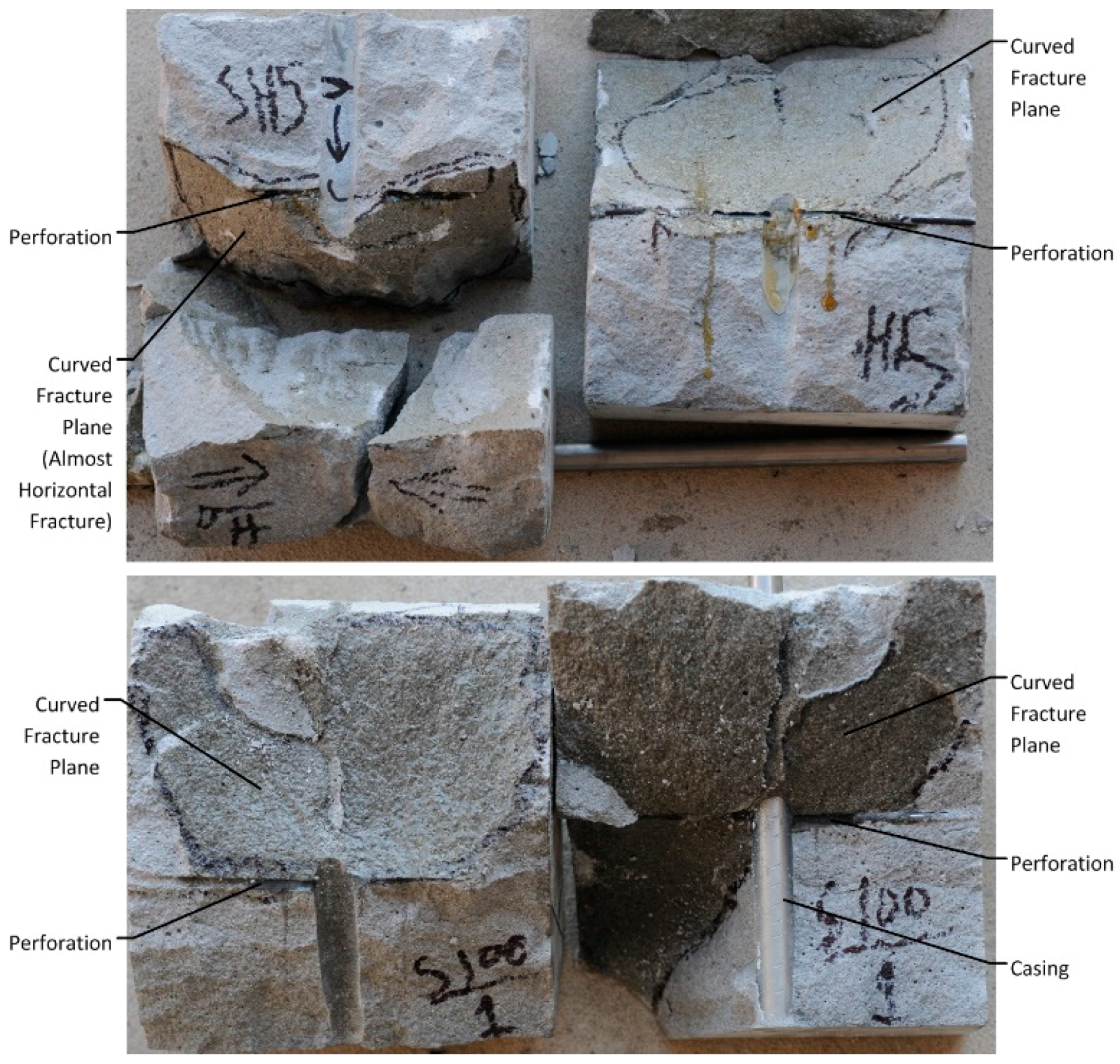
Figure 6 shows the fracture geometries of the samples fractured in tests H-2 and H-3. As it is seen in this figure, in test H-2 almost a vertical fracture (along PFP) was developed. However, test H-3 resulted in a curved fracture plane, where the fracture was initiated from the perforations in an angle with respect to PFP, but each wing of fracture propagated in a curved path towards the PFP. As it is described in Table 5, tests H-4, SL-1, SL-3, and SH-1 also experienced curved fracture planes. However, the angles (with respect to PFP) at which the fractures were initiated from the perforations, as well as the curvature of the fracture planes were not the same in all these tests.
For instance, as it is shown in Figure 8, in test H-4 two-wing fractures were initiated from each perforation. However, the bottom fracture was initiated at a larger initiation angle than the top fracture. Moreover, the bottom fracture propagated almost in the horizontal plane, which is perpendicular to the vertical stress, while the top wing grew in a curved path towards the PFP. Test SL-1 also resulted in two-wing fractures; however, the fracture initiation angle for this test is less than that of test H-4. Additionally, the top and bottom fractures in test SL-1 experienced less curvature in comparison to the fractures in test H-4.
In order to recognize the relationship between fracture initiation angle and propagation geometry with the injection flow rate and viscosity, it is helpful to recall the product of these two parameters (Q × μ). The product of injection flow rate and viscosity is calculated for each test and presented in Table 6. Although by increasing the product value, higher initiation and break down pressures were recorded, it appears that some of the tests have the same product values, while their fractures’ geometries are different. For instance, tests H-4 and SL-1 have almost the same product value (see Table 6); however, their fracture geometries are not the same.
To clarify this controversy, it is worthwhile to mention that the product of injection flow rate and viscosity represents the amount of energy applied to pressurize the wellbores and create the fractures. However, because every test had a particular injection rate and fluid viscosity, the wellbore pressurization time was not the same for all tests. For example, sample H-4 was pressurized with a flow rate of 5 cc/min using honey with a viscosity of 20 Pa.s, while sample SL-1 was tested using silicone oil with a viscosity of 97.7 Pa.s and a flow rate of 1 cc/min. Hence, sample H-4 was pressurized much faster than sample SL-1, since a much less viscous fluid was injected into its wellbore at a higher flow rate. This is while both samples had almost the same level of fracturing energy (Q × μ), but sample H-4 had received this energy at a faster rate. Therefore, it would be significantly helpful to divide the fracturing energy by the time interval at which this energy was supplied to each sample. Energy divided by time would introduce a new parameter which is considered to be the fracturing power as given below:
P f r a c t u r i n g = Q × μ t
The time interval t is considered to be the wellbore pressurization time in each test. This time interval starts with the moment when the wellbore begins to pressurize and ends when the fracture breaks down.
Table 6 summarizes the fracturing energy, pressurization time, and fracturing power as well as the characteristics of fracture geometry for each test, excluding test H-1 in which no fracture was developed in the sample. Each fracture geometry is characterized by an initiation angle, which is the angle at which the fracture was initiated from the perforation with respect to the PFP. Additionally, the fracture propagation plane is also generally characterized as either planar or curved.
Comparing the fracturing powers of tests H-4 and SL-1 indicates why the fracture geometry in test H-4 had a larger initiation angle and a more curved fracture plane (see Figure 8), although they have almost equal fracturing energy of about 16 × 10−7 N.m. The same result is concluded when comparing the fracturing power and geometries in the other tests. For example, test SH-1 experienced a fracturing power of almost 140 × 10−10 N.m/s, and as a result a curved fracture with an initiation angle of 75 degrees was created in this test.
In contrary, tests H-2, SL-2 and SH-2 had very low fracturing powers and consequently, an almost planar fracture was initiated from their perforations and propagated in the vertical direction, along PFP. Thus, generally, it is concluded that the fracturing energy could not be directly related to the fracture initiation and propagation geometry. Nevertheless, the fracturing power could be associated with the fracture geometry very well.
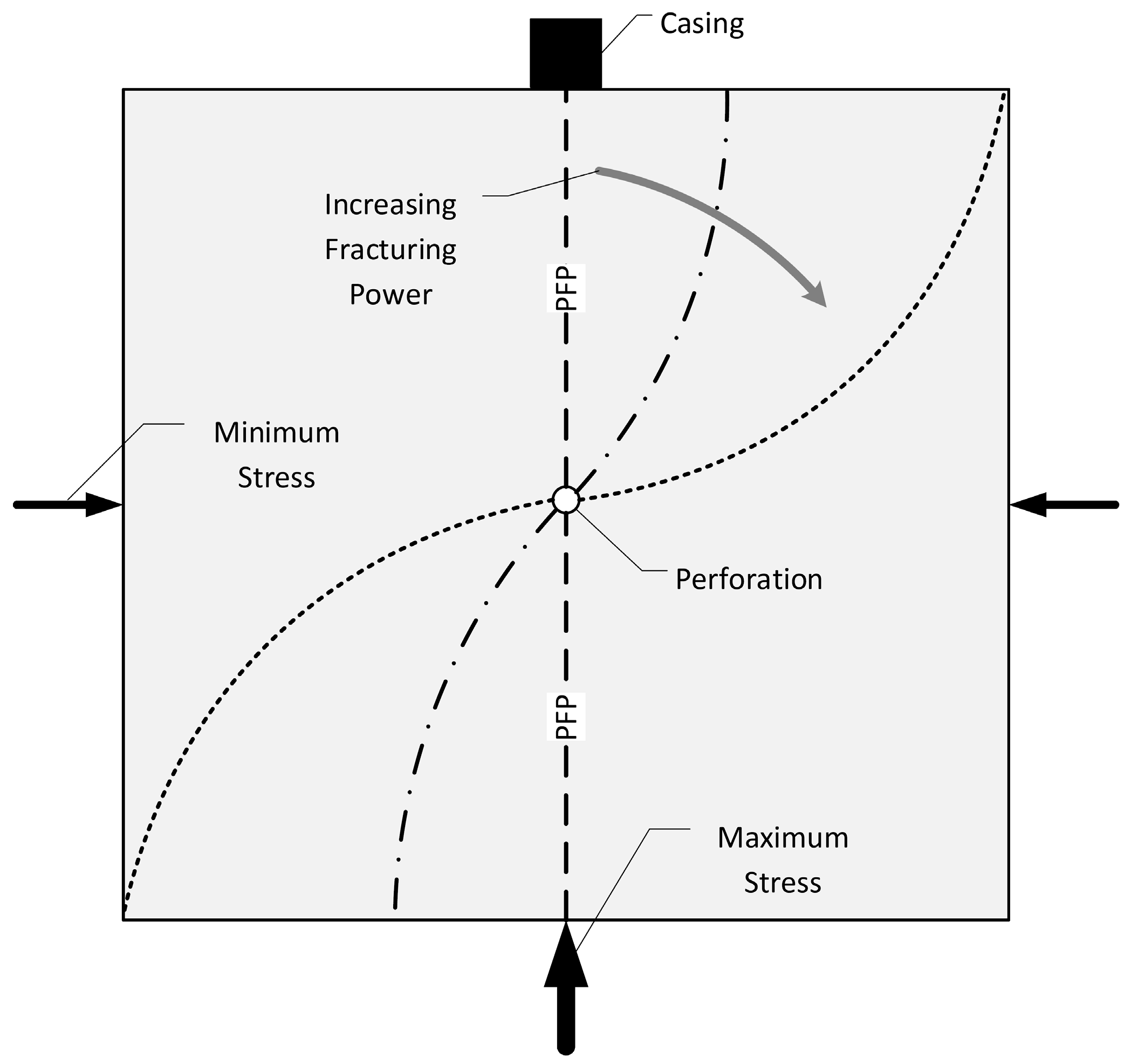
Basically, as it is demonstrated in Figure 9, by increasing the fracturing power supplied to the sample, the wellbore pressurization rate increases. Consequently, the fracture initiation angle increases. This means that at higher fracturing power, fractures could be initiated from the perforations in a direction which is perpendicular to higher stress components (herein vertical stress). Accordingly, the fracture propagation would have a longer curved path so that it could get aligned with the PFP (the plane to which the minimum stress is perpendicular).
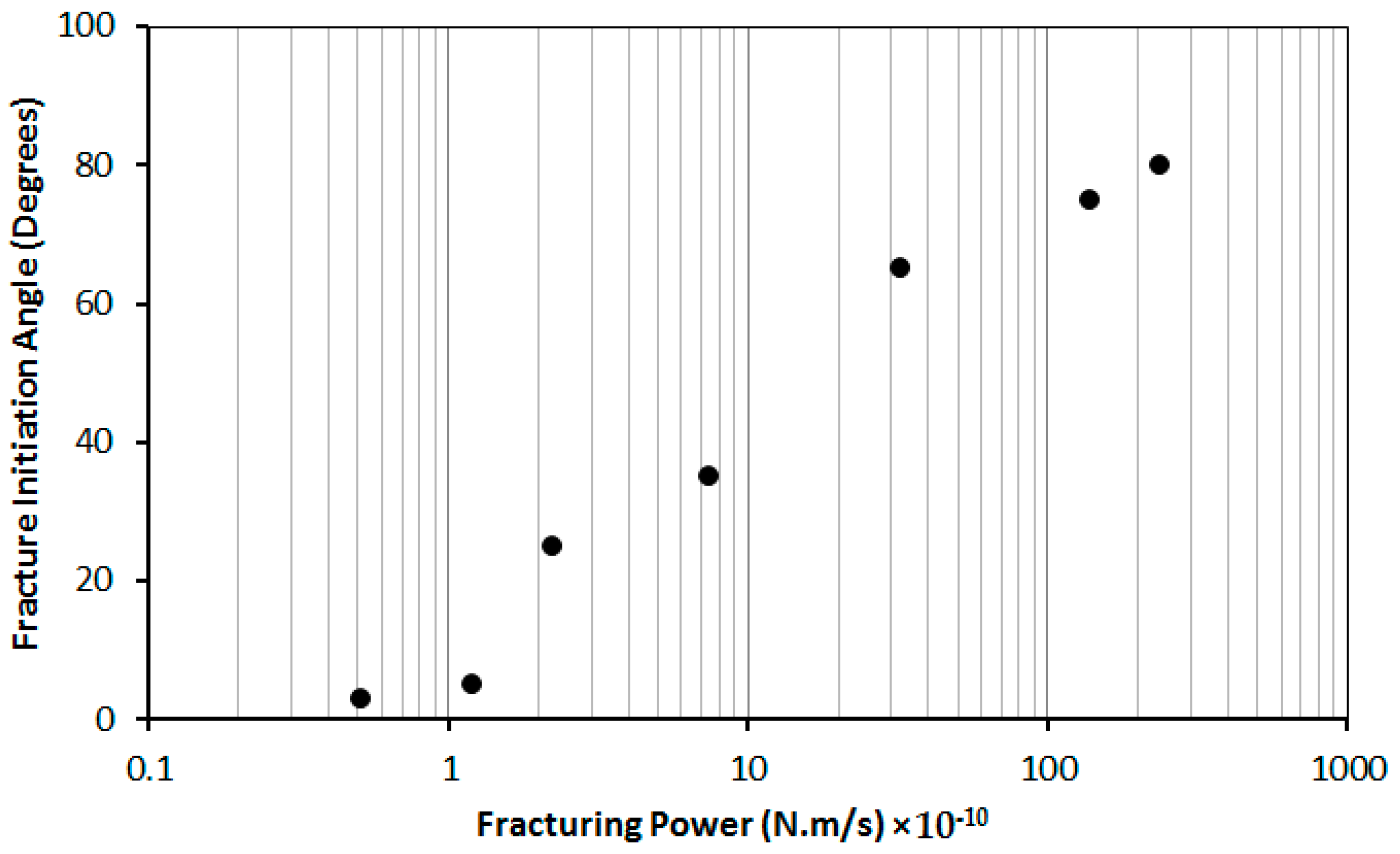
A graph of fracture initiation angle versus fracturing power shows that there is a linear relationship between these two parameters on a semi-log plot (Figure 10). Such relationship could introduce the following general equation:
λ = a log P f + b
where λ is the initiation angle, Pf is the fracturing power, and a and b are the constants of the equation, that may depend on sample’s properties and the applied principal stresses. Further experiments and analysis are required to justify this equation and to include the effects of fracturing power on the fracture propagation curvature, because the curvature of the fracture appears to be closely related to its initiation angle.
It should be noted that test SL-3 had the lowest fracturing power of 0.06 × 10⁻¹⁰ N.m/s; however, in this test a single fracture was not developed. The injection flow rate was as low as 0.05 cc/min in this test. Such low flow rate, which was applied to a high viscous fracturing fluid (97.7 Pa.s), resulted in very long pressurization time (14,000 s). Consequently, a very low fracturing power was supplied to the sample, which led to multiple fracturing over the course of wellbore pressurization. This is in good agreement with the results obtained in the experimental study conducted by Van de Ketterij [15]; while they only considered the product of injection flow rate and viscosity and did not indicate the influence of fracturing power. Therefore, test SL-3 is the only test that appears not following the relationship between the fracturing power and the fracture propagation geometry, and this is due to the very low power that led to multiple fracturing.

5.3.3. Casing Effect

As it was mentioned earlier, in most of the tested samples, the fractures were initiated from the perforations in an angle with respect to a vertical plane (PFP). Then the tip of the fracture turned towards the PFP in some distance away from the wellbore wall. The fracturing power is now believed to be the main reason for the curvature of the fractures. However, the existence of the casing also played an important role. The steel casing has different elastic moduli with respect to the synthetic sample. Generally, the elastic Young’s modulus of the casing is larger than that of the sample.
Therefore, if one compares a pressurized open wellbore with a pressurized cased wellbore, assuming that both of them are at the same pressure, the open wellbore would experience larger radial stress on the wellbore wall. This is due to the fact that when the casing is pressurized, the whole fluid pressure would not be transferred to the surrounding wellbore’s material because casing would have less radial displacement in comparison to the open wellbore [20]. As a result, less radial stress would be transferred to the wellbore wall. Lower radial stress would accordingly lead to higher tangential stress, so the casing can affect the wellbore and accordingly the perforation stress distribution. Consequently, the fracture initiation and break down pressures would be affected.
Authors have previously conducted some fracturing experiments on the same synthetic samples [12]. However, in the previous study, there was no casing and the perforations were drilled in the openhole. It is noteworthy that the diameter of the perforations in the aforementioned study was 2 mm larger than the current study. However, based on the elastic stress distribution equation for the analysis of the stress profile around a circular cavity [31], the radius of the perforation does not have an effect on its stress distribution. Therefore, the results of the two experimental studies could be compared with each other.
A comparison between the fracture initiation and break down pressures of the planar fracture in this study with those of similar fracture geometries in the previous study reveals that the existence of the casing has significantly increased the fracturing pressures. As an example, in test SL-2, where a planar vertical fracture was propagated, the fracture initiation and break down pressure were 17.44 MPa and 18.19 MPa respectively. Similar planar vertical fracture geometry in the previous study (tests 2–3 in [12]) was developed at an initiation pressure of 6.89 MPa and the corresponding break down pressure was 7.62 MPa. This comparison clearly illustrates the impact of the casing on wellbore and perforation stress distributions, and consequently the increase in the fracturing pressures.

6. Conclusions

In order to analyze the fracturing pressure-time, curves a new methodology is introduced in this study to predict the fracture propagation time directly from the pressure-time curves. This methodology assisted in the indication of the time at which the fracture tip reached the boundary of the sample. Accordingly, the rest of the pressure data after this time was considered as representing the flow of the fracturing fluid through the propagated fracture. Therefore, this methodology greatly improved the results’ interpretations.
Experimental results demonstrated that as the product of viscosity and injection flow rate increases, higher fracture initiation and break down pressure would be recorded. This product value has the same dimension as energy. Therefore, it is considered to represent an energy term, named as fracturing energy. Hence, as the fracturing energy increases the fracturing pressures would increase accordingly.
Nevertheless, it was observed that the fracture initiation angle and near wellbore propagation geometry may not be directly related to fracturing energy. Therefore, a new parameter was introduced by dividing the fracturing energy by the wellbore pressurization time, named as fracturing power (Equation (6)). It is observed that as the fracturing power rises, the fracture initiation angle increases and a more curved fracture plane would be propagated.
It is also observed that casing has a significant effect on the wellbore and perforation stress distribution. As a result, larger fracture initiation and break down pressures would be expected in a cased perforated completion, in comparison to a perforated openhole wellbore. Additionally, the casing would cause a vertical fracture to deviate from the wellbore and propagate in a curved path toward the PFP.
The strength properties of the cement sheath play an important role in the hydraulic fracturing mechanism in a cased perforated wellbore. Low shear strength cement sheath may result in creation of a micro-annulus. Accordingly, the hydraulic fracture would propagate in the annulus between the casing and the wellbore wall. As a result, the wellbore pressure would decrease and consequently there would be no or little chance of the creation of hydraulic fracture in the formation.

Author Contributions

Seyed Hassan Fallahzadeh conceived and designed the experiments; Seyed Hassan Fallahzadeh and Ashton James Cornwell performed the experiments and analyzed the data; Md Mofazzal Hossain and Vamegh Rasouli contributed towards reagents/materials/analysis; Seyed Hassan Fallahzadeh wrote the paper, and Md Mofazzal Hossain and Vamegh Rasouli revised and improved the paper.

Conflicts of Interest

The authors declare no conflict of interest.

References

  1. Cleary, M.; Johnson, D.; Kogsb, H.; Owens, K.; Perry, K.; Pater, C.; Alfred, S.; Holger, S.; Mauro, T. Field implementation of proppant slugs to avoid premature screen-out of hydraulic fractures with adequate proppant concentration. In Proceedings of the Low Permeability Reservoirs Symposium, Denver, CO, USA, 26–28 April 1993.
  2. Davidson, B.; Saunders, B.; Robinson, B.; Holditch, S. Analysis of abnormally high fracture treating pressures caused by complex fracture growth. In Proceedings of the SPE Gas Technology Symposium, Calgary, AB, Canada, 28–30 June 1993.
  3. Aud, W.; Wright, T.; Cipolla, C.; Harkrider, J. The effect of viscosity on near-wellbore tortuosity and premature screenouts. In Proceedings of the SPE Annual Technical Conference and Exhibition, New Orleans, LA, USA, 25–28 September 1994.
  4. Lehman, L.; Brumley, J. Etiology of multiple fractures. In Proceedings of the SPE Production Operations Symposium, Oklahoma City, OK, USA, 9–11 March 1997.
  5. Behrmann, L.; Elbel, J. Effect of perforations on fracture initiation. J. Pet. Technol. 1991, 43, 608–615. [Google Scholar] [CrossRef]
  6. Abass, H.; Brumley, J.; Venditto, J. Oriented perforations-a rock mechanics view. In Proceedings of the SPE Annual Technical Conference and Exhibition, New Orleans, LA, USA, 25–28 September 1994.
  7. Gulrajani, S.N.; Romero, J. Evaluation and modification of fracture treatments showing near-wellbore effects. In Proceedings of the European Petroleum Conference, Milan, Italy, 22–24 October 1996.
  8. Behrmann, L.; Nolte, K. Perforating requirements for fracture stimulations. SPE Drill. Complet. 1999, 14, 228–234. [Google Scholar] [CrossRef]
  9. Hossain, M.; Rahman, M.; Rahman, S. Hydraulic fracture initiation and propagation: Roles of wellbore trajectory, perforation and stress regimes. J. Pet. Sci. Eng. 2000, 27, 129–149. [Google Scholar] [CrossRef]
  10. Atkinson, C.; Eftaxiopoulos, D. Numerical and analytical solutions for the problem of hydraulic fracturing from a cased and cemented wellbore. Int. J. Solids Struct. 2002, 39, 1621–1650. [Google Scholar] [CrossRef]
  11. Fallahzadeh, S.H.; Shadizadeh, R.S.; Pourafshary, P. Dealing with the challenges of hydraulic fracture initiation in deviated-cased perforated boreholes. In Proceedings of the SPE Trinidad and Tobago Energy Resources Conference, Port of Spain, Trinidad, 27–30 June 2010.
  12. Fallahzadeh, S.; Rasouli, V.; Sarmadivaleh, M. An investigation of hydraulic fracturing initiation and near-wellbore propagation from perforated boreholes in tight formations. Rock Mech. Rock Eng. 2015, 48, 573–584. [Google Scholar] [CrossRef]
  13. Romero, J.; Mack, M.; Elbel, J. Theoretical model and numerical investigation of near-wellbore effects in hydraulic fracturing. In Proceedings of the SPE Annual Technical Conference and Exhibition, Dallas, TX, USA, 22–25 October 1995.
  14. Daneshy, A. Experimental investigation of hydraulic fracturing through perforations. J. Pet. Technol. 1973, 25, 1201–1206. [Google Scholar] [CrossRef]
  15. Van de Ketterij, R.G. Optimisation of the Near-Wellbore Geometry of Hydraulic Fractures Propagating from Cased Perforated Completions. Ph.D. Thesis, Delft University of Technology, Delft, The Netherlands, 2001. [Google Scholar]
  16. Van Ketterij, R.; De Pater, C. Impact of perforations on hydraulic fracture tortuosity. SPE Prod. Facil. 1999, 14, 117–130. [Google Scholar] [CrossRef]
  17. Perkins, T.; Weingarten, J. Stability and failure of spherical cavities in unconsolidated sand and weakly consolidated rock. In Proceedings of the SPE Annual Technical Conference and Exhibition, Houston, TX, USA, 2–5 October 1988.
  18. Fallahzadeh, S.H.; Rasouli, V.; Sarmadivaleh, M. Experimental investigation of hydraulic fracturing in vertical and horizontal perforated boreholes. In Proceedings of the 47th US Rock Mechanics/Geomechanics Symposium, San Francisco, CA, USA, 23–26 June 2013.
  19. Mindess, S.; Young, J.F.; Darwin, D. Concrete; Prentice Hall: Upper Saddle River, NJ, USA, 2003. [Google Scholar]
  20. Fallahzadeh, S.; Rasouli, V. The impact of cement sheath mechanical properties on near wellbore hydraulic fracture initiation. In Proceedings of the ISRM International Symposium-EUROCK, Stockholm, Sweden, 28–30 May 2012.
  21. Rasouli, V. A true triaxial stress cell (ttsc) used for simulations of real field operations in the lab. True Triaxial Test. Rocks 2012, 4, 311. [Google Scholar]
  22. Min, S.; Sastry, S.; Balasubramaniam, V. Compressibility and density of select liquid and solid foods under pressures up to 700 mpa. J. Food Eng. 2010, 96, 568–574. [Google Scholar] [CrossRef]
  23. Bunger, A.P. Near-surface hydraulic fracture. Ph.D. Thesis, University of Minnesota, Minneapolis, MN, USA, 2005. [Google Scholar]
  24. De Pater, C.; Weijers, L.; Cleary, M.; Quinn, T.; Barr, D.; Johnson, D. Experimental verification of dimensional analysis for hydraulic fracturing. SPE Prod. Facil. 1994, 9, 230–238. [Google Scholar] [CrossRef]
  25. Weijers, L. The Near-Wellbore Geometry of Hydraulic Fractures Initiated from Horizontal and Deviated Wells. Available online: http://repository.tudelft.nl/islandora/object/uuid:44f71145-b331-43af-a3d5-32916fd7333c/datastream/OBJ/view (accessed on 21 November 2016).
  26. Lhomme, T.P.Y. Initiation of Hydraulic Fractures in Natural Sandstones. Ph.D. Thesis, Delft University of Technology, Delft, The Netherlands, 2005. [Google Scholar]
  27. Mack, M.G.; Warpinski, N. Mechanics of hydraulic fracturing. In Reservoir Stimulation; Wiley: New York, NY, USA, 2000. [Google Scholar]
  28. Detournay, E. Propagation regimes of fluid-driven fractures in impermeable rocks. Int. J. Geomech. 2004, 4, 35–45. [Google Scholar] [CrossRef]
  29. Bourgoyne, A.T.; Millheim, K.K.; Chenevert, M.E.; Young, F. Applied Drilling Engineering; Society of Petroleum Engineers: Richardson, TX, USA, 1986. [Google Scholar]
  30. Nelson, E.B. Well Cementing; Elsevier Science: Amsterdam, NY, USA, 1990. [Google Scholar]
  31. Fjar, E.; Holt, R.M.; Raaen, A.; Risnes, R.; Horsrud, P. Petroleum Related Rock Mechanics; Elsevier: Amsterdam, NY, USA, 2008. [Google Scholar]
Figure 1. Sand grain size distribution for synthetic samples.
Energies 10 00359 g001
Figure 2. A schematic of 150 mm cubic sample with a cased wellbore at the center and two 4 mm perforations that are perpendicular to the axis of the wellbore and at an angle of 180° from each other (all dimensions are in mm).
Energies 10 00359 g002
Figure 3. A view of the TTSC with the horizontal platen and the horizontal hydraulic rams (top), syringe pumps for the hydraulic rams and fracturing fluid injection (Middle), and a synthetic sample accommodated in the TTSC using the spacer blocks (Bottom).
Energies 10 00359 g003
Figure 4. A schematic of fracturing fluid injection set-up.
Energies 10 00359 g004
Figure 5. Fracturing pressures recording and wellbore pressurization rate for test SL-1.
Energies 10 00359 g005
Figure 6. Test H-3 (top) and H-2 (Bottom) fracture geometries.
Energies 10 00359 g006
Figure 7. A view of the broken sample H-1 after the test, where fracturing fluid has propagated a fracture in the adhesive (top), and the corresponding fracturing pressure graph which shows a typical multi-fracturing mechanism (bottom).
Energies 10 00359 g007
Figure 8. Fracture geometries of tests H-4 (top) and SL-1 (bottom).
Energies 10 00359 g008
Figure 9. A schematic of the fracture initiation angle and propagation geometry in response to variation in the fracturing power.
Energies 10 00359 g009
Figure 10. The relationship between the fracture initiation angle and the fracturing power.
Energies 10 00359 g010
Table 1. Properties of the synthetic sample and the adhesives used for sample preparation.
Mechanical PropertiesValueUnitTesting Methodology
UCSUni-axial compressive strength79.5MPaUnconfined compression test *
ToTensile strength3.5MPaBrazilian tensile test *
KICFracture Toughness0.78MPam0.5Semi-Circular bend test *
Elastic Properties
νPoisson’s ratio0.19-Unconfined compression test *
EYoung’s Modulus27.74GPaUnconfined compression test *
Adhesives Shear Strength
τoSelleys Liquid Nails1.1MPaSandblasted aluminum lap shear **
τoSuper Strength Araldite26MPaSandblasted aluminum lap shear **
Physical Properties
ρbBulk density2047Kg/m3Density measurement test
ρgGrain density2500Kg/m3Density measurement test
φPorosity13.5%Two Boyle’s cells
KPermeability0.019mDTransient gas flooding
* Presented by [18]; ** Provided by manufacturer.
Table 2. Fracturing fluids’ physical properties.
Fracturing FluidViscosity (Pa.s)Specific DensityCompressibility (1/psi)Maximum Frictional Pressure Loss (MPa) ***
Honey201.36 **1.00 × 10⁻⁴ **0.18
Poly DMS-T5197.7 *0.977<9.43 × 10−50.4
Poly DMS-T56586.8 *0.978<9.43 × 10−51.04
* Viscosities reported at 34.5 MPa by the producer; ** Obtained from [22]; *** These values were calculated based on the maximum injection rate of each fluid.
Table 3. Dimensionless toughness number for each fracturing fluid flowing at a particular flow rate.
Fracturing FluidViscosity (Pa.s)Flow Rate (cc/min)Dimensionless Toughness (κ)
Honey2010.65
Honey2020.58
Honey2050.49
Poly DMS-T5197.70.050.69
Poly DMS-T5197.70.10.61
Poly DMS-T5197.710.42
Poly DMS-T56586.80.10.37
Poly DMS-T56586.810.25
Table 4. Fracturing tests’ parameters and main results.
Test No.Fluid Viscosity (cP)Injection Rate (cc/min)Initiation Pressure (MPa)Breakdown Pressure (MPa)Propagation Time (s)
H-120,0001.008.969.10----
H-220,0001.0012.8214.19320
H-320,0002.0010.6911.41669
H-420,0005.0015.2418.68636
SL-197,7001.0018.4019.96340
SL-297,7000.1017.4418.19936
SL-397,7000.057.98–14.378.16–14.65499
SH-1586,8001.0032.7535.65364
SH-2586,8000.1028.2732.72460
Table 5. Brief description of the fracture geometries.
Test No.Test Description and Fracture Geometry
H-1The fracturing Fluid (honey) created several fractures in the solid adhesive, which had filled the annulus between the casing and the wellbore. Eventually, the fractures reached the bottom of the annulus and the fluid leaked out.
H-2This sample was initially intended to be fractured by a flow rate of 1 cc/min; however, after 3100 s of injection, no fracture was initiated. Therefore, the flow rate was then increased to 2 cc/min. Consequently, the wellbore pressure increased and eventually a vertical, almost planar, fracture perpendicular to the direction of minimum stress was initiated and propagated from each perforation tunnel. The two fractures did not link up at the vicinity of the wellbore, probably due to high stress concentration around the wellbore.
H-3From each perforation a two-wing fracture was propagated along the perforation axis. However, the initiated fractures were not vertical at the perforation wall, and had an angle of about 35° with respect to the vertical plane. Both fractures propagated downwards and upwards in the sample in a curved path, and in a distance away from the wellbore they turned towards the vertical plane (PFP).
H-4Similar to the previous test, curved fractures were initiated from the perforations, and then turned towards the PFP. The lower wing of the fracture in this test made an angle of about 80° with respect to the vertical plane; however, it turned towards a plane where less normal stress was applied.
SL-1Almost similar to the two previous tests, from each perforation a two-wing fracture was created in an angle of 65° with respect to the vertical plane. Then, in some distance away from the wellbore, the fractures turned towards the PFP.
SL-2An almost planar fracture, making an angle of 3° with respect to PFP, was developed from both perforations, and propagated mostly towards the bottom of the sample.
SL-3This test exhibited multiple fracturing. In addition, a two-wing fracture was developed almost against the maximum stress, initiating from one of the perforations. Then one of its wings propagated and changed its direction towards a vertical plane, which was nearly perpendicular to the minimum stress. The other perforation just initiated a small fracture.
SH-1A two-wing fracture was developed almost against the maximum stress, initiating from one of the perforations. Then one of its wings propagated and turned towards the PFP.
SH-2An almost planar vertical fracture, making an angle of 25° with respect to PFP, was propagated from one of the perforations. The other perforation created a fracture which also developed towards the vertical plane and perpendicular to the minimum stress direction.
Table 6. Fracturing tests’ energy, pressurization time, power, and fracture geometry characteristics.
Test No.Injection Rate (m3/s) ×10−8Fluid Viscosity (Pa.s)Q × μ (Fracturing Energy) (N.m) ×10−10Pressurization Time (s)Fracturing Power (N.m/s) ×10−10Fracture Initiation Angle (°)Fracture Propagation Geometry
H-21.6720.0376331001.25Planar
H-33.3320.066679007.435Curved
H-48.3320.016,66770238.180Curved
SL-11.6797.716,28350032.665Curved
SL-20.1797.7162832000.53Planar
SL-30.0897.781414,0000.060 to 70Curved
SH-11.67586.897,800700139.775Curved
SH-20.17586.8978044002.225Almost Planar

