1. Introduction
Phase change materials (PCMs) are suitable products for thermal management solutions, because they store and release thermal energy during the process of melting and freezing.
They are also very effective in providing thermal barriers or insulation, for example in temperature controlled transport.
PCM dispersions based on salts can be very interesting for applications in the building sector, thanks to the high latent heat of fusion and the temperature at which this transition occurs.
In such applications, they are enclosed in boards for the thermoregulation of internal environments. Panels can cover walls, floors, or ceilings, therefore large quantities of such materials are required.
This need imposes limits in the choice of materials with regards to economic aspects, making it useful to address the recycling of waste materials, for example the Glauber’s salt that is obtained as a byproduct from the disposal process of lead batteries.
The recovery is carried out by the crystallization of sulphate, which also allows for the elimination of traces of heavy metals, toxic to the environment and damaging to health.
In particular, in the phase of the pastel desulfurization in which the lead sulphate is treated by using the carbonate or hydroxide of sodium, the following reactions take place [
1,
2]:
Due to its thermal properties, the Glauber’s salt has been one of the first salt hydrates to be considered suitable for applications in the building sector [
3].
Glauber salt’s transition is a peritectic phase change where the solid Glauber salt produces a liquid phase consisting of a sodium sulphate solution and a solid phase consisting of Na
2SO
4 [
4].
In reference [
5], data for the pure Glauber’s salt are available: the enthalpy of fusion is equal to 251.2 kJ/kg, the phase transition temperature is 32.4 °C, and the specific heat of the solid and liquid phase are equal to 2.09 kJ/(kg·K) and 3.35 kJ/(kg·K), respectively.
However, during initial investigations, problems of stability have been highlighted and, as a consequence, difficulties in long term performances.
These problems were mainly due to two phenomena common to many other hydrated salts: supercooling and phase segregation. The first prevents the release of heat at a defined temperature, while the second, due to the incongruent melting, limits the stability of the structure which is manifested by a progressive reduction of the enthalpy of fusion. The solutions proposed in the literature involve adding a nucleating substance [
6] and a rheological modifier [
7], in addition to an excess of water whose function is to counter the low solubility of the salt [
8].
When additives are mixed with pure PCMs, a heterogeneous mixture occurs.
The chemical, physical, and thermal properties are completely different with respect to the pure compounds, and they have to be evaluated experimentally for such heterogeneous mixtures.
The study presented in this paper is based on the characterization and the thermal analysis of two compositions with different percentages of Glauber’s salt, obtained by using bentonite as a thickener and borax as a nucleating agent. This paper presents results related to the compositional weight percentage of sodium sulphate of 25% and 31%, and of 67% and 60% of water chosen after a selection of different compositions, previously tested with the aim of achieving interesting PCM thermal properties. The objective is to analyze their effect on the enlargement of the solidification interval, on the lowering of the solidification temperature, and on the fusion enthalpy and stability in comparison to the pure salt. Since the samples are dispersions, it was necessary to identify the most appropriate type of mixing, opting for sonication as the more effective method as opposed to the magnetic stirring technique in reducing the size of the aggregates [
9]. Two samples were prepared for each composition by varying the sequence of addition of the reagents. Each sample was analyzed successively by means of the T-history method for the determination of their thermal properties, and by using optical techniques to obtain information on their stability.
The purpose of the paper was to introduce a methodology able to predict the stability of Glauber’s salt based PCMs in a relatively short time with a significant amount of samples, in order to guarantee that any inhomogeneity will be taken into account. By such a method, it is possible determine how both compositions and methods of preparation affect the properties of PCMs. The results have also been used in order to obtain further information about the thermal performance of the studied PCMs.
2. Materials and Methods
2.1. Reagents and Preparation of the Samples
For the preparation of the samples the following reagents were utilized: distilled water, sodium sulfate 99.5% purity, borax 99.5% purity, potassium chloride 99% purity, purchased from Carlo Erba (Milan, Italy), and bentonite, provided by Sigma-Aldrich Italia (Milan, Italy).
Table 1 shows the two analyzed compositional weight percentages.
The compositional weight of bentonite and borax were selected thanks to preliminary experimental activity, carried out with the aim of investigating the optimal range of composition of the additives able to guarantee that the phase change occurs in the temperature range of interest for applications in building fields. As a consequence, the ratios between sodium sulphate and water are equal to 0.37 for sample 1 and 0.52 for sample 2.
The samples have been made using a sonicator UP200S provided by Hielscher (Teltow, Germany); sonotrode S14 with a diameter of 14 mm), proceeding with 0.8 cycles of impulse followed by 0.2 s of pause at 100% of the length amplitude. Each composition (in total 100 g) has been obtained by the application of two different modalities:
Modality (1): water and bentonite were sonicated for 10 min. After the addition of salts, the dispersion sonicated for a further 30 min.
Modality (2): water and salts are sonicated for 30 min, and in a second step the bentonite was added and sonication was applied for 10 min.
The samples will be identified in the paper following the nomenclature shown in
Table 2.
During sonication an increase of temperature to 70 °C was observed in all modalities. For this reason, all the samples were cooled to 40 °C in the thermostable bath, in order to apply the T-history method and optical analysis.
It was possible to observe that all the samples appeared solid at temperatures lower than 19 °C and liquid for temperature higher than 31 °C.
Sample preparation, as well as thermal and stability analyses, were replicated more than two times in order to guarantee a good reproducibility of the results. The data scattering was calculated for the thermal analysis and the optical stability analysis in terms of mean percentage error between the sets of data.
2.2. Thermal Analysis: T-History Method
The thermal analysis was carried out by using the T-history method [
10] in the temperature range from 10 °C to 40 °C. The original setup has been improved by using a refrigerated thermostat FOC 215 l from Velp Scientifica, (Usmate Velate (Monza Brianza), Italy)), as also suggested by Stankovic et al. [
11], coupled in our case with the Software TEMPSoft™ supplied from Velp Scientifica, (Usmate Velate (Monza Brianza), Italy)) to program the heating and cooling ramps continuously, in order to obtain an adequate control of the environmental conditions, following the assigned function.
Duran® test tubes (height of 16 cm and diameter of 1 cm) were used to store the PCM and reference material during the T-history analysis. Water was used as reference substance, because it does not show phase change in the investigated temperature range. The distance between test tubes was large enough to avoid any interference during heat transport.
The T-history method was applied by decreasing the temperature from 40 °C to 10 °C with a step of 1°/min, then the samples stayed at 10 °C for two hours, and after they were heated to 40 °C (step of 1°/min). The cycle was repeated four times. Temperatures inside the PCM test tube as well as inside the reference (water) test tubes were continuously measured with resistance temperature detectors (RTDs) PT100, a miniature sensor RTD with high accuracy, with a diameter of 0.5 mm and length of 100 mm (able to guarantee fast and reproducible results). Two tests were performed for each sample.
PCM mixture samples in the liquid phase, after sonication and cooled to 40 °C, were immediately placed in the refrigerated thermostat and RTD probes were inserted in the test tubes. Simultaneously, test tubes with reference substances were heated at 40 °C and the RTD probes were lodged in the refrigerated thermostat that will represent the environment at which the temperature is called the ambient temperature.
Temperature profiles during the heating and cooling cycles were continuously measured, following the method proposed from Zhang and Jiang [
10] and T-history curves were prepared. As reported in the literatures [
10,
11,
12], cooling curves were used for the evaluation of ∆
H. The results are therefore presented with reference to the method of Marin et al. [
12], in which in addition to the enthalpy of fusion, the representation of the enthalpy-temperature trend is shown in the examined range. Such representation takes into account that PCMs do not have homogeneous compositions and, therefore, they have a rather wide solidification range. The enthalpy–temperature curve has been obtained by considering the changes in enthalpy in small temperature ranges according to Equation (3):
where
mw,
mt, and
mp are the mass of water, test tube, and PCM, respectively (kg);
cpw and
cpt are the specific heat of water and the test material (kJ/(kg·K)); for the
ith step, ∆
Ti is the temperature range (°C) with average value
Ti, to which the enthalpy variation ∆
hp(
Ti) (kJ/kg) corresponds;
Ii is the integral with respect to time of the difference in temperature between the PCM and environment;
Ii’ is the integral with respect to time of the difference in temperature between the water and environment.
The latent heat of solidification was obtained as [∆
hp(
TiS) − ∆
hp(
TfS)] where
TiS is the initial temperature of solidification calculated as the maximum value reached after sub-cooling and
TfS is the final temperature, calculated according to as a point of inflection on the cooling curve of PCM [
13].
The specific heat of PCM in the liquid (
cpl) and solid state (
cps) was calculated in reference to the article of Marinas, where the gradients of the two straight lines are observable in the enthalpy versus temperature trend [
12,
13].
2.3. Kinetic of Destabilization
PCMs made of Glauber’s salt and additives are dispersions. For this reason, they are subject to destabilization phenomena during the time that could affect their thermal properties.
Generally, these phenomena concern particle migration that determines sedimentation and creaming, or variation of their dimensions (flocculation and coalescence).
Destabilization could affect the thermal performance of PCMs, and consequently it is important to predict these phenomena from the beginning. When sedimentation, clarification, or flocculation occur, the texture of the materials is changed, and as a consequence the thermal conductivity, thermal capacity, heat of fusion or solidification, and density change: the system could be compared to a side or series resistance system, in terms of heat exchange. Fusion or solidification phenomena occur in different ways in the material and that could affect the effectiveness of the thermal behaviour of the PCM.
Destabilization phenomena are not visible to the human eye when they are characterized by low kinetics, and only some sophisticated optical methods and instruments, such as the Turbiscan, are able to detect them from the initial stages [
14,
15,
16].
The operating principle is based on multiple light scattering. The instrument scans samples with a volume of about 25 mL and draws transmission (T) and backscattering (BS) profiles along the height of the test cell. The scan can be repeated for a long time, and at fixed intervals of time. The more the profiles are distinguished from the initial one, the more unstable the dispersion.
In the case of opaque dispersions, as those considered in this investigation, the backscattering profile is more effective than the transmission profile that is null.
The
BS percentage along the test cell provides information regarding the homogeneity of the sample, but in order to easily identify the phenomena in the samples, it is recommended to use the Delta mode. One of the profiles (by default, the first one) is used as a “blank” corresponding to the initial dispersion state of the sample. This profile is then subtracted from the other profiles, thus emphasizing the variations [
17].
In
Table 3, examples of the results in terms of delta backscattering (∆
BS) obtained with Turbiscan are presented with reference to the most important destabilization phenomena that occur with inhomogeneous PCMs.
By means of comparing the profiles in time, the instrument determines the destabilization kinetics based on the computation of the Turbiscan Stability Index (
TSI). The
TSI is a computation directly based on the raw data of the transmission and backscattering signals. The superposition of the BS profiles is indicative of stability while their deviation across time increases with the instability of the dispersions. The
TSI can be determined by using the comparison of the scans at a given time. In particular, the
TSI is determined for the
ith step [
17]:
- (1)
by comparing every scani(h) of a measurement to the previous one scani−1(h), on the selected height h;
- (2)
by dividing the result by the total selected height (
H) in order to obtain a result which does not depend on the quantity of product in the measured cell:
The
TSI computation sums up all the variations in the sample, to give as a result a unique number reflecting the destabilization occurring in a sample. The higher the
TSI, the stronger the destabilization in the sample. Consequently, an asymptotic value of
TSI could mean two things:
- (1)
The material is stable: in this case, TSI has a constant value from the initial time and during the entire analysis. Usually, this happens for homogeneous materials.
- (2)
The material is unstable at the beginning and becomes stable after a long time (more than 24 h): in this case, the asymptotic value could be observed after a long time because the original sample changed its texture. As a consequence, the material probably became stable but with a very different texture, with different overall thermal properties, like conductivity, thermal capacity, density, or other physical properties: It became a different material with respect to the initial one and its thermal behavior (i.e., as a PCM) needs to be recalculated.
In the investigation proposed in this paper, the analyses were conducted considering a period of 24 h and the temperature was fixed at the maximum value in the observation range (40 °C) in which the sample remains in the liquid phase.
3. Results and Discussion
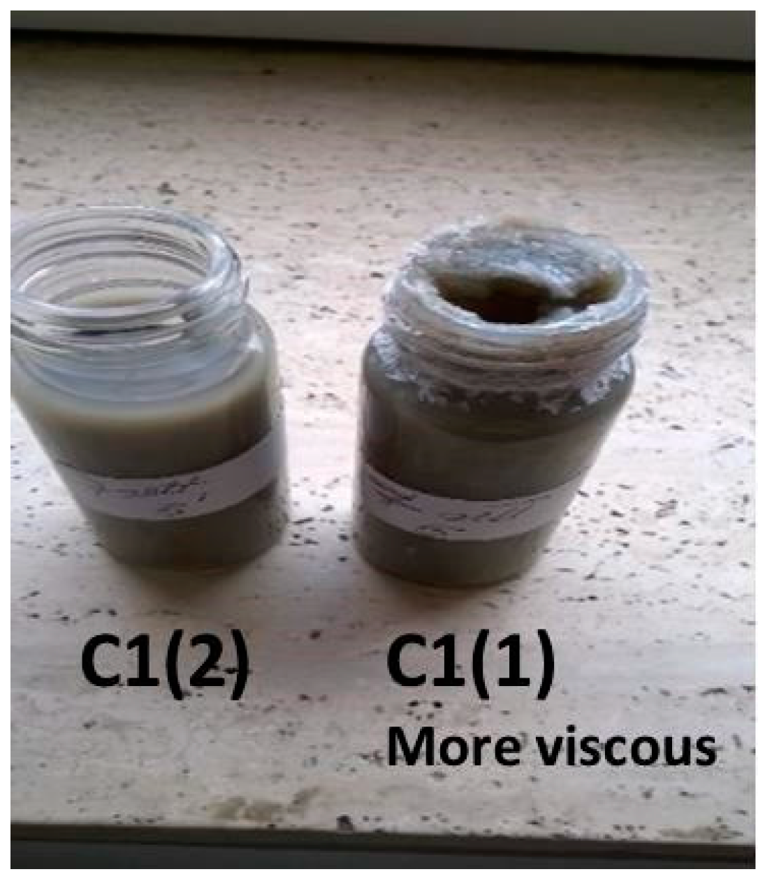
By preparing the sample following modalities 1 or 2, it is possible to observe significant and visible differences in their textures. In particular, the first sample (both for C1 and C2) has an appearance more viscous than the second.
Figure 1 shows the comparison between the compositions C1(1) and C1(2).
Sample C1(1) appears like a dough, with a rheological behavior intermediate between a liquid and a solid system. On the contrary, sample C1(2) appears as a liquid. To the naked eye, it appears to have a more homogeneous texture than C1(1), where the inhomogeneity is more evident.
3.1. Thermal Analysis of the Samples
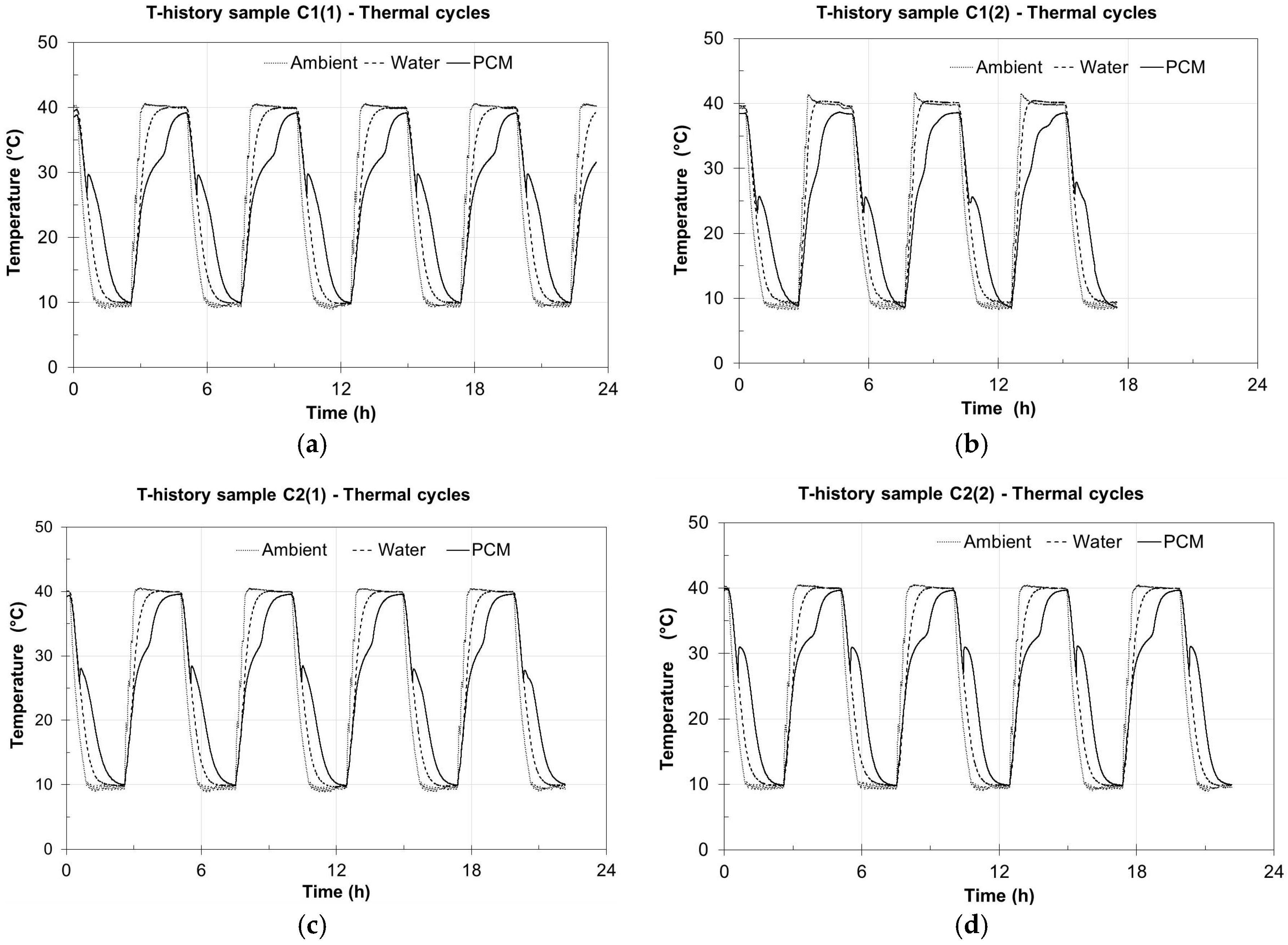
In
Figure 2, the results of the T-history method applied at each sample C
i(
j), are reported. They depict the heating and cooling cycles obtained in the refrigerated thermostat (the environment) where the temperature was changed from 40° to 10 °C following the imposed function, as described in
Section 2.2.
In the figure, the temperature evolution of the refrigerated thermostat where the samples are lodged (ambient temperature) as well as the temperature evolution in the PCM and water (reference substance) are reported.
It is possible to see the supercooling limited to 2–3 °C and the repeatability of the cycles. As reported in the literatures [
10,
11,
12,
13], cooling curves have been used for the second part of the method, then by considering the cooling curves and Equation (3), the enthalpy versus temperature curves were determined for all the samples. The results obtained for sample C1 are shown in
Figure 3.
The thermal properties of the first sample, estimated by considering the method described in
Section 2.2, are summarized in
Table 4.
The first composition has a percentage of sodium sulphate equal to 25%. In both modalities of preparation, a decrement of the temperature range of solidification with respect to the value of the pure salt is observed. This phenomenon could be correlated to the presence of additives that also determines an extension of the solidification interval. Such range of temperature is greater for the first composition and marks a major degree of inhomogeneity. Furthermore, it need to be taken into account that for sample C1(1), the water and bentonite were first mixed. Thus, it can be predicted that part of the water will be trapped by the bentonite silicate layers, thus reducing the water available to mix with the sodium sulphate, affecting melting temperature range.
The specific heats, for the solid and liquid phase, are larger than those for the pure Glauber’s salt reported in the introduction [
5]. In fact the excess of water is known to elevate the specific heat.
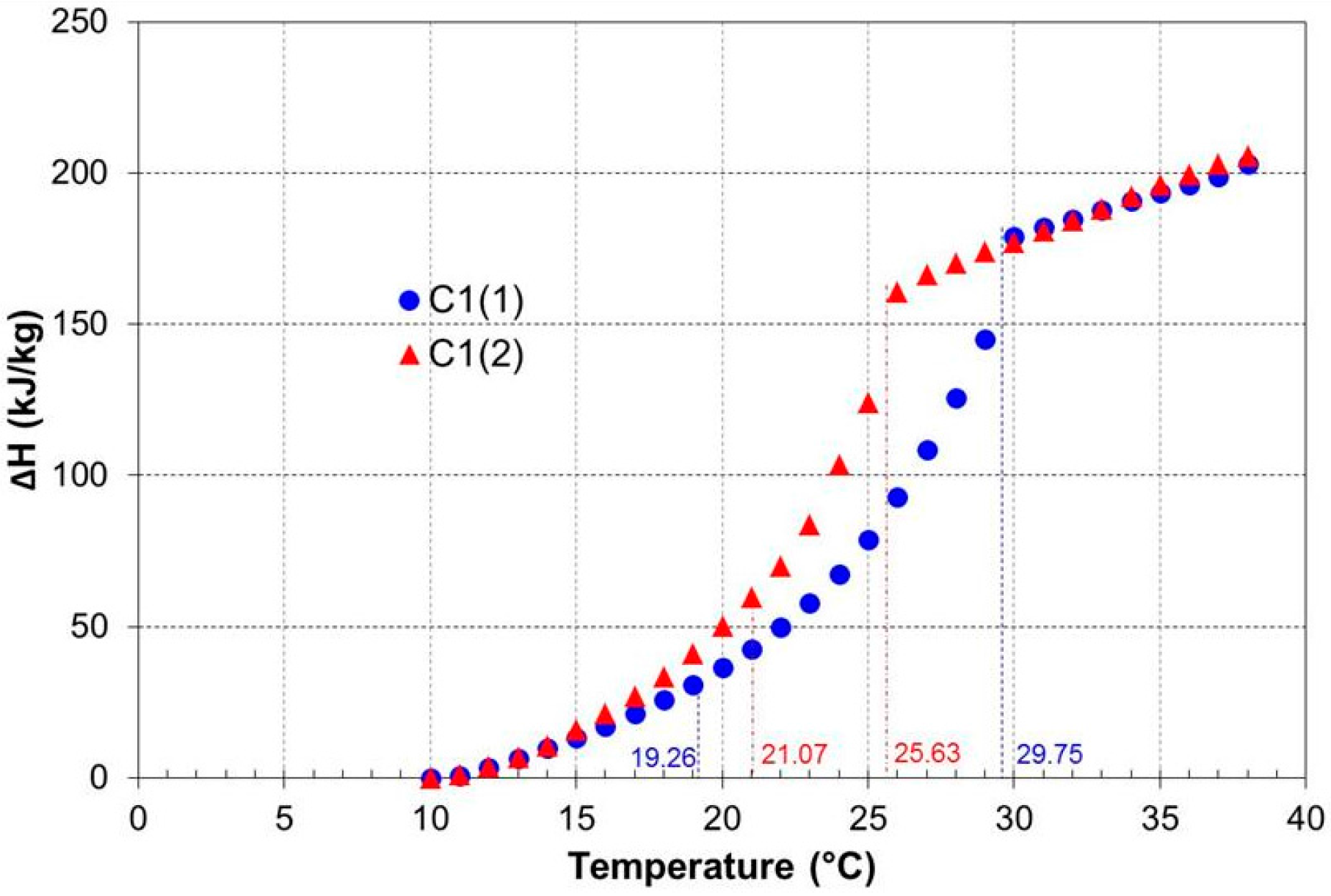
In
Figure 4, the enthalpies of fusion of the two samples with composition 2 are compared and a significant difference in the values is noticed.
The thermal properties of the second sample are presented in
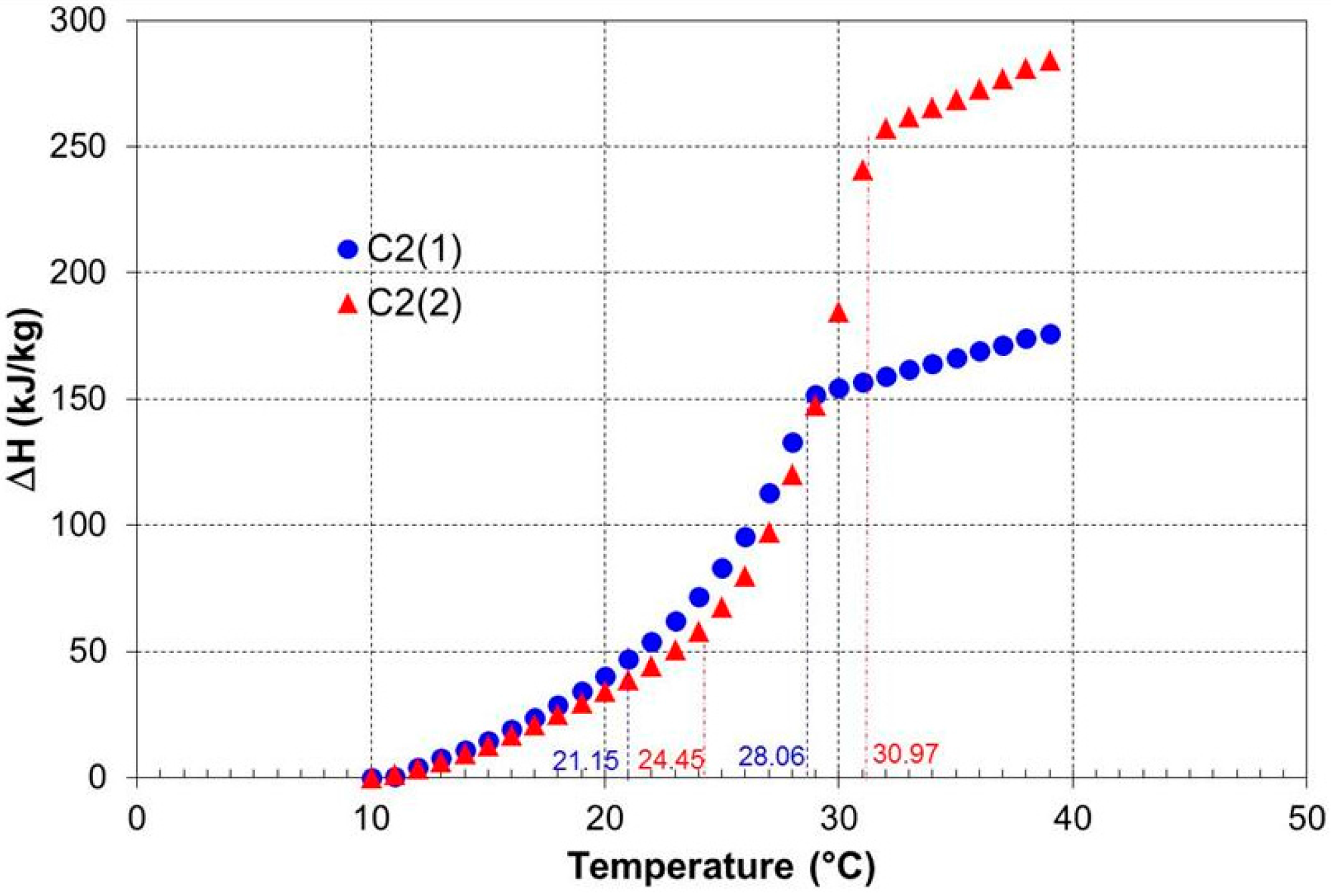
Table 5.
Both the C2 compositions contain a percentage by weight of sodium sulphate equal to 31%, however the sample obtained by modality 1, C2(1), presents a thermal performance less effective than that of sample C2(2) and also than that of the C1 samples that contain a minor percentage of sodium sulphate (25%). This result is probably due to the high viscosity of C2(1) that reduces the efficacy of the sonication process: the same sonication power is not able to effectively break up the anhydrous sodium sulphate, reducing the formation of the decahydrate form (Glauber’s salt) and therefore the final thermal performance of the sample.
In all the analyzed compositions, the size of supercooling is 2–3 °C and it can be considered very reduced in comparison to the values higher than 15 °C indicated in the literature for the pure salt [
18], revealing the efficacy of the adopted nucleant.
Further consideration could be performed taking into account the phase diagram of the sodium sulphate–water system, as proposed by Biswas [
19]. In order to apply such a diagram, the amount of Na
2SO
4 has been calculated and the corresponding theoretical melting temperature values have been estimated for each sample. It is important to notice that the phase diagram is relative to a system without additives, therefore the amount of sodium sulphate has been recalculated assuming a system without bentonite and borax.
For sample 1 where the amount of Sodium sulphate is 25%, the corresponding value for the phase diagram has been estimated at 27.17%. That corresponds to a condition in which the anhydrous sodium sulphate crystals are not expected in the studied range of temperature (10–40 °C). Furthermore, the theoretical transition temperature is 25 °C, and the value is within the experimental range reported in
Table 4 for both C1(1) and C1(2).
For sample 2, the amount of charged sodium sulphate is 31% and, assuming a system without additives, the corresponding value is 34.07%. In the phase diagram, this value corresponds to a limit condition and, beyond this value, the formation of anhydrous sodium sulphate is expected. With this value in the phase diagram, the theoretical transition temperature could be expected to be 32 °C. This value is more similar to that obtained in
Table 5, because the additives play a more significant role during the activity of Glauber’s salt as a PCM. With the amount of sodium sulphate and water reported in
Table 1, it is possible to expect that the availability of water is greater for sample 1 than for sample 2. Bentonite and sodium sulphate compete for water. Sample 1 has enough water for both, and consequently, the theoretical melting point is in the observed range of temperature
Tis and
Tfs for both samples C1(1) and C1(2). On the other hand, for sample 2 where less water is available, the modality plays a more significant role. Modality 1 gives an immediate possibility for bentonite to hydrate itself with water: less water remains for the Glauber’s salt formation. Consequently, the temperature range where melting occurs is closer to a system where a smaller amount of hydrated salt is present. With modality 2, Glauber’s salt could be easily obtained during the first sonication. Residual water becomes available for the hydration of bentonite. As a consequence, thermal performance closer to Glauber’s salt could be reached, as confirmed for the temperature range shown in
Table 5.
Finally, the reproducibility of the data was confirmed from the evaluation of the mean error percentage between the data sets of each sample. With reference to the data shown in
Figure 3 and
Figure 4, mean errors range from 4.45% and 5.56%.
3.2. Stability Analysis of the Samples
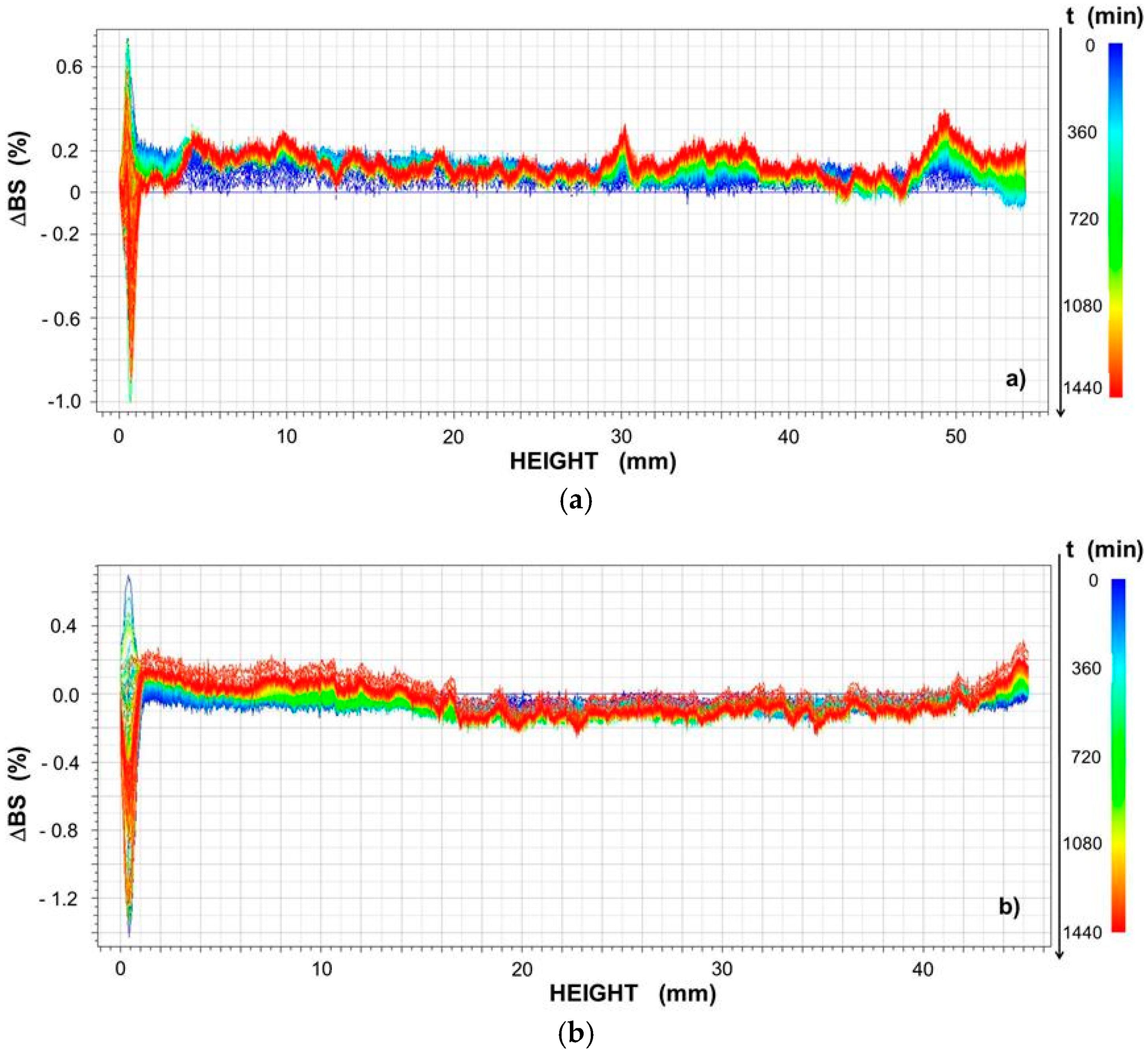
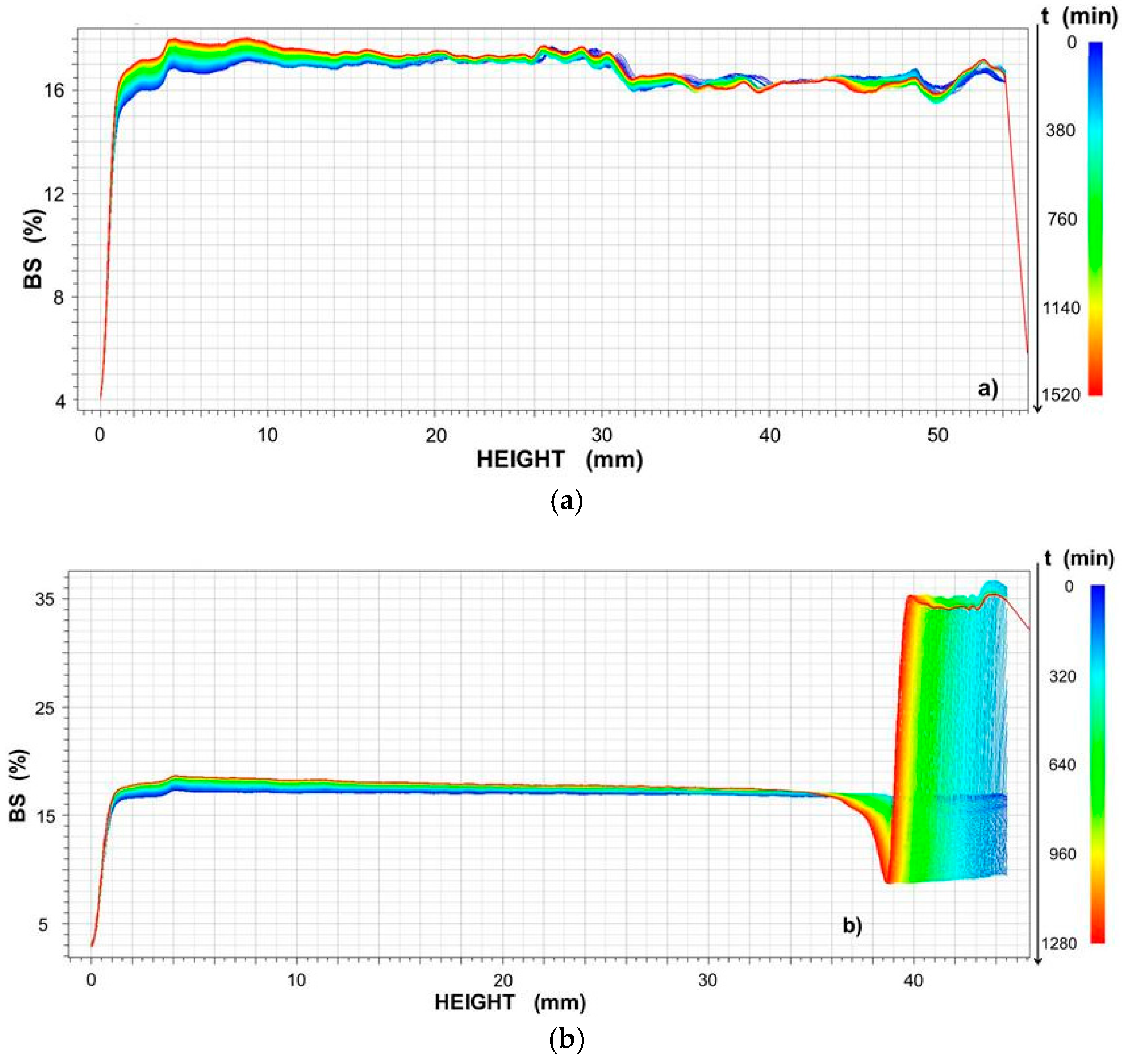
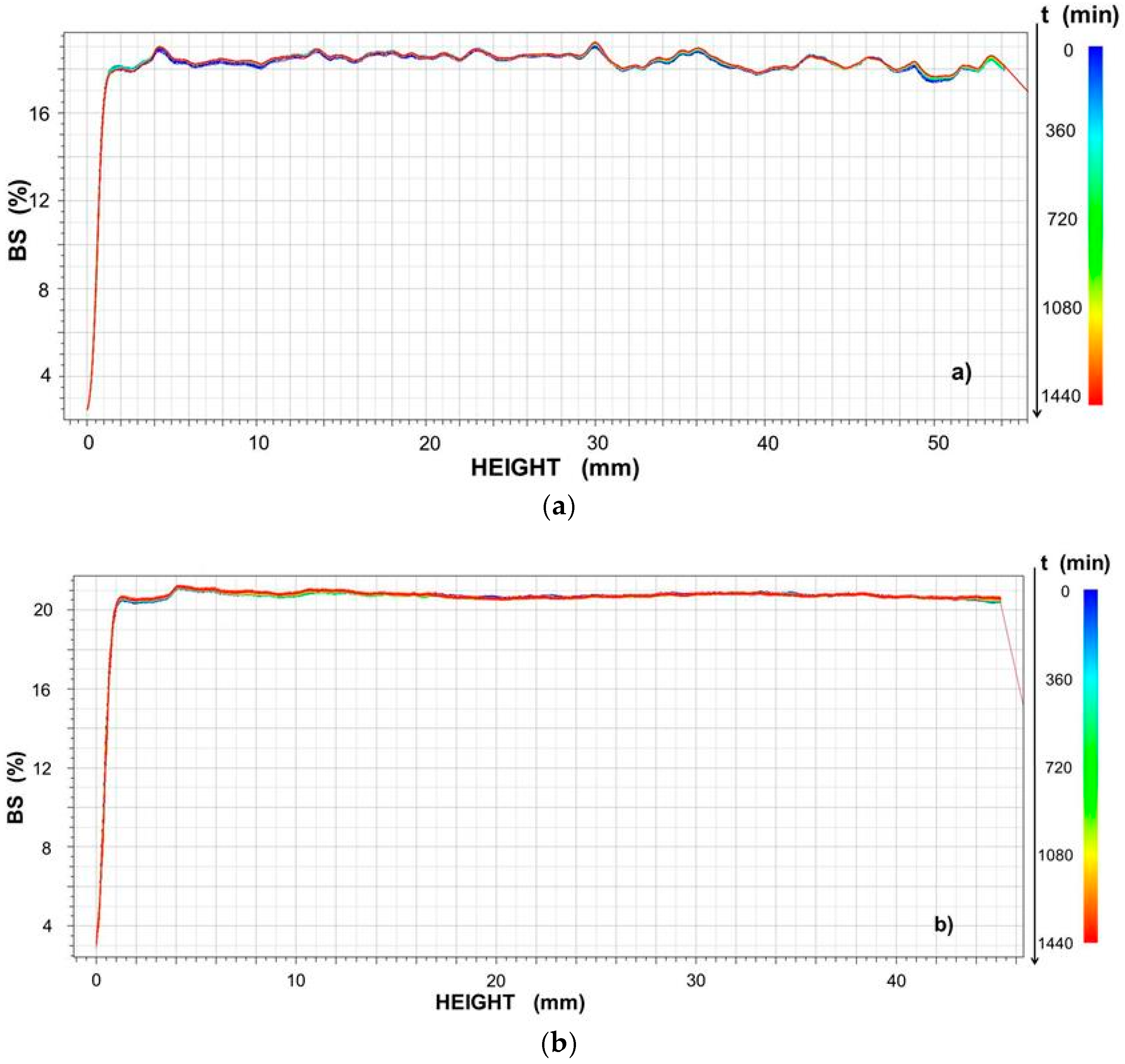
The
BS profiles of the samples C1(1) and C1(2) are shown in
Figure 5.
The composition C1(1) shows in each scan a percentage of the BS variable along the height of the cell, revealing the inhomogeneity of the sample. The composition C1(2) is rather homogeneus until 36 mm height; from this point, sedimentation and creaming phenomena become evident.
Thus the sonication is more effective on the second dispersion that is less viscous. As a consequence, its solidification range (shown in
Figure 3) is more limited (the first one is 10.49 °C, the second one is limited to 4.56 °C) while the total Δ
H of the process is comparable.
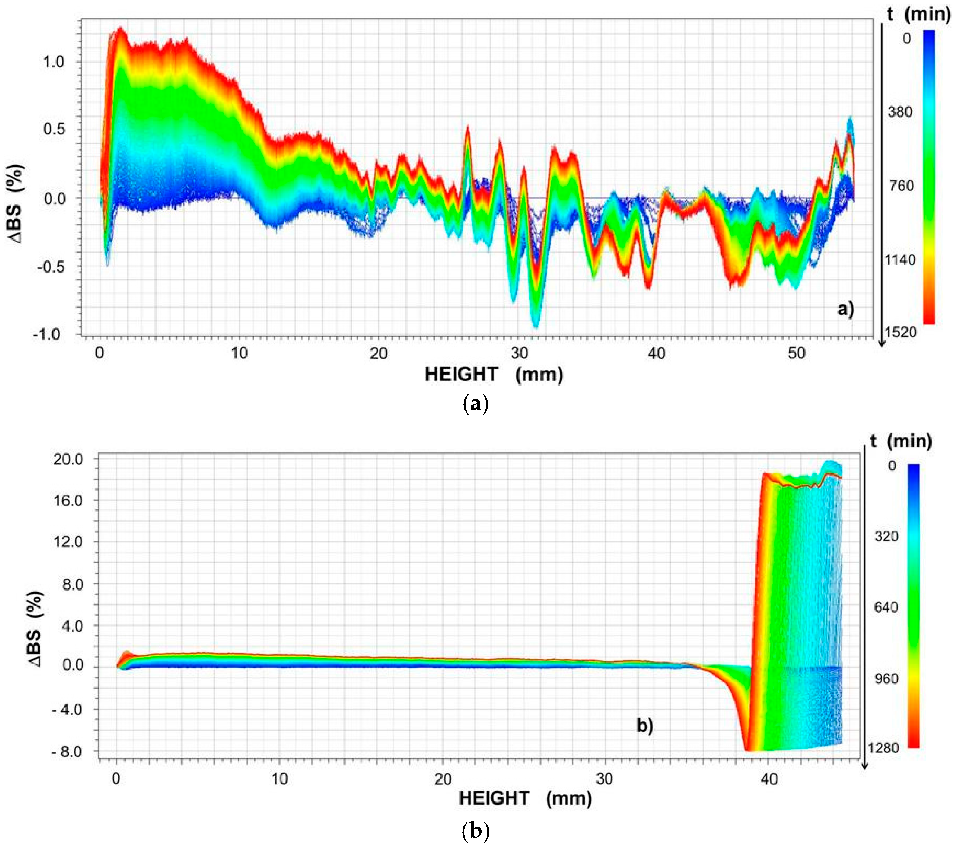
∆
BS profiles are presented in
Figure 6 in order to underline the nature of these phenomena.
In sample C1(1), the flocculation phenomena are dominant and the shift of the trends up and down during the time depends on the particle diameter, smaller or larger than the incident radiation [
17]. In sample C1(2), sedimentation, creaming, and flocculation are observed. The presence of sedimentation and creaming is probably due to the lower viscosity of the dispersion.
Also for the composition C2, the second method of preparation makes the dispersions more homogeneous, as shown in
Figure 7.
Unlike the previous case, a minor effect on the solidification temperature interval is observed, as shown in
Figure 3 and
Figure 4.
However for this composition, in both sequences of reagent additions, only the flocculation is reported. The absence of sedimentation and creaming is probably correlated to a higher viscosity of composition C2(2) in comparison to C1(2) thanks to the higher contents of bentonite and the lower percentage of water.
∆
BS percentages, obtained for composition C2, are presented in
Figure 8 for both modalities of preparation.
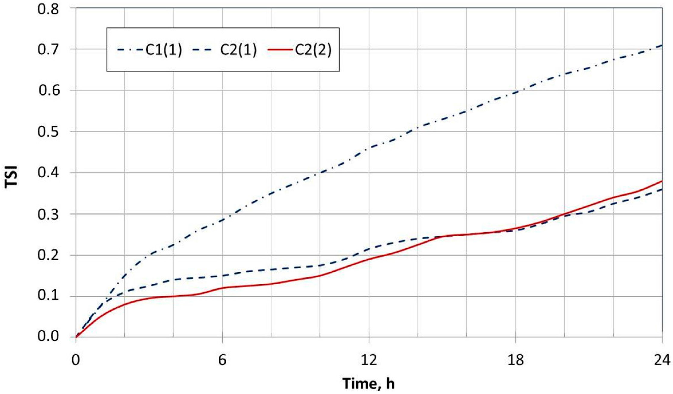
The stability analysis has been quantified by considering the
TSI behavior and comparing the trends obtained in 24 h. As already stated, such an index could be used as a measure of the progressive destabilization of the system. It is important to notice that the optical testing obtained by Turbiscan is disruptive and non-repeatable. Thus, it is possible to test each sample one time during the 24 h period, with a scan of 5 min. It seems interesting to do the comparison between the repeated samples in terms of the
TSI data scattering: the mean values of the errors in terms of
TSI behaviour has been found, ranging from 6.25% to 10.2%. In
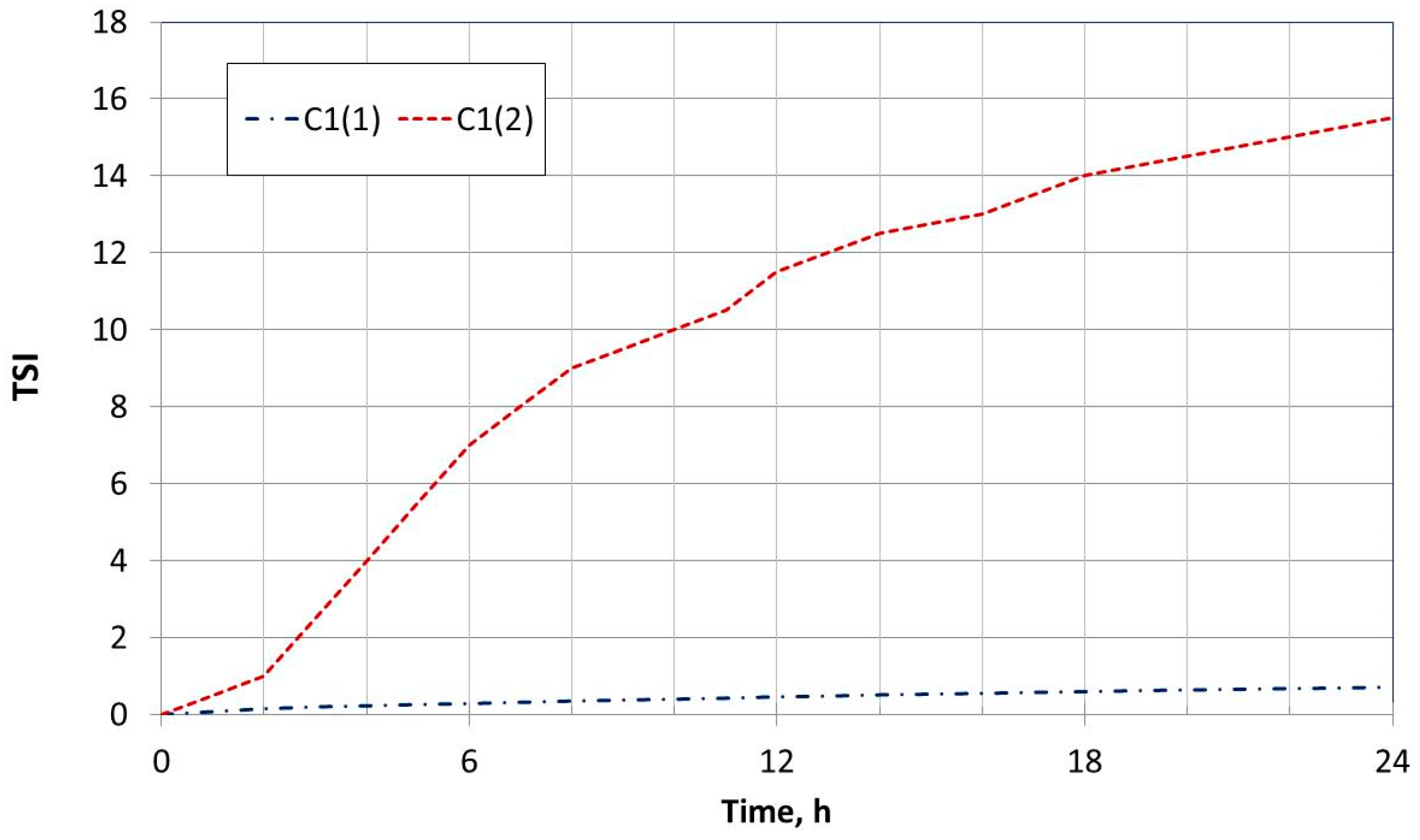
Figure 9, the
TSI values are reported with reference to sample C1 for the two different preparation modalities. It appears evident that modality 2 is not adequate for the preparation of Glauber’s salt, as discussed by observing the features of the samples in
Figure 2.
TSI values increase progressively until 15, for sample C1(2). This trend indicates that the sonication of water and bentonite is preferable in the first step of preparation of such composition.. That allows us to achieve more homogeneous samples.
In order to evaluate the influence of composition,
TSI behavior has been reported in
Figure 10 for samples C1(1), C2(1), and C2(2). That allows us to compare the influence of composition on stability (samples C1(1) and C2(1)) and the influence of modality in the cases where more concentrated solutions were used (samples C2(1) and C2(2)). It is interesting to note that the
TSI for C1(1) is almost double the
TSI of C2(1). No significant difference can be observed for C2(1) and C2(2). That could be due to the fact that the sample C2 is characterized by a higher thickener (as bentonite)/water ratio, able to guarantee a greater stability of the solution.
In any case, samples C2(1) and C2(2) are more stable than C1(1). However, sample C2(2) offers better thermal performances in comparison to C2(1), and consequently it should be preferred for further studies.
4. Conclusions
In this paper, samples of PCMs based on Glauber’s salt dispersions have been studied, by changing their composition and modality of preparation with the aim of estimating, by the T-history method, their thermal properties, and by means of optical methods, their stability.
It has been observed that both compositions and modalities of preparation significantly affect the phase change enthalpy, melting temperature range, and structural stability.
This is due to how the components are distributed in the PCM solutions at different thermal conditions, affecting both dispersion and viscosity as also verified for other families of heterogeneous materials [
20,
21]. This is more relevant when PCMs are subject to numerous thermal cycles or when crystallization or supercooling are involved.
In particular, the nucleant selected in order to limit the supercooling has produced satisfactory results in all the analyzed cases, as it is able to reduce this phenomenon to a few degrees celcius. With reference to the thickener, it was observed that the stability of the dispersion improves for the samples that present a greater bentonite/water ratio, thanks to the higher viscosity.
In defining the optimal composition of Glauber’s salt and additives, the results underlined that the thermal performances and the stability of the dispersion cannot be defined by considering only the percentage of the composition. The final properties depend on the preparation method and in particular, on the sequence used for adding the reagents and on the viscosity of the mixture.
In any case, the aim of this paper is to provide an example of a procedure useful for testing the quality of inhomogeneous samples by considering both thermal performance and stability. The different compositions and modalities of preparation have been tested in order to underline the different behaviors of PCMs in relation to these variables.
We suggest the use of this method as a way to characterize PCMs and, consequently, as a method of preparation and composition optimization.
Of course, further studies should be carried out at different lifetimes, depending on the purpose of the investigation. However, it is important to verify how the preparation methodology can affect the initial thermal properties and the stability of samples.


