Tuning the Complexity of Photovoltaic Array Models to Meet Real-time Constraints of Embedded Energy Emulators

Abstract

Reproducibility of experimental conditions is a fundamental requirement for designing energy efficient, self-sustainable wireless sensor networks (WSNs). At the same time, it represents a significant challenge because of the variability and the unpredictability of many energy harvesting sources, and because of the dynamic operating conditions of the devices to which energy is supplied. Energy source emulation is considered a suitable solution to enable the exploration of the design space of networked embedded systems. However, in order to guarantee the compatibility with real-time performance of resource-constrained embedded platforms, particular attention has to be paid to the complexity of the models. In this paper, we propose an approach aimed at tuning the complexity of models of photovoltaic (PV) arrays implemented on a target embedded emulator, featuring low cost and small form factor. Experimental results performed on different models of PV array, show that the proposed solution is flexible and accurate enough to meet the real-time constraints of typical sensor networks applications without impairing the precision in the emulation of the energy sources.

1. Introduction

Energy efficient design of embedded systems plays a pivotal role in the increasing diffusion of pervasive devices for many different application scenarios, ranging from environmental monitoring to smart grids, from building automation to surveillance. Indeed, energy consumption in battery-operated devices directly impacts the system lifetime and it clearly represents a limitation in all cases where interventions for batteries substitution should be avoided or kept to a minimum.

To overcome these obstacles, several research directions and strategies have been proposed. Among them, the main contributions can be considered: (i) the design of novel electronic devices with ultra low-power capabilities, resulting in hardware with increased performance and/or decreased power consumption levels; (ii) the introduction of dynamic power management techniques, which adapt the power drained by a system (and its performance) to different workloads (e.g., by putting devices into low-power modes and saving energy); and (iii) the use of renewable energy sources, which makes it possible to replenish batteries and/or directly supplying power. This last option introduces a significant paradigm shift, namely from energy consumption minimization to energy-rate (i.e., power) minimization [1].

Energy harvesters based on photovoltaic (PV) arrays with reduced form factor have been recently proposed with the aim of increasing the energetic autonomy of embedded systems. In the context of wireless sensor networks (WSNs), such an autonomy is of utmost importance because of the limitations imposed by resource-constrained platforms typically adopted [2,3,4]. As a matter of fact, a target of energy-harvesting WSNs (EH-WSNs) is the so-called energy-neutral operation (ENO). The ENO of a sensor network is a working point of the network obtained by matching harvested energy and computational loads to achieve long-term energetic sustainability and, ultimately, a (theoretically) unlimited lifetime [4,5,6].

The design of hardware–software embedded systems, protocols, and algorithms capable of meeting the design goals of self-sustainable EH-WSNs still remains, however, a challenging task. Energy harvesting sources are in fact inherently unpredictable and subject to complex dynamics. Moreover, supplied loads are frequently subject themselves to frequently changing operating conditions: load impedance and, subsequently, drawn energy, can vary because of dynamic power management policies (e.g., a switch to a low power mode of the radio transceiver or of the microcontroller unit during idle periods) or because of the normal activity of the application (e.g., a particular event that triggers a given actuation command in a monitoring task). Finally, workloads are unpredictable even in a controlled environment because of the effects of packet overhearing and interference.

These issues make the design and test of EH-WSNs particularly problematic because of the difficulty to obtain reproducible and realistic testing conditions. On one hand, exploration of the design space can be carried out by means of simulation, which allows reproducibility at the cost of approximating, to a different extent, real-world operating conditions. On the other hand, one can resort to the implementation on testbeds, which permit the evaluation of design solutions in a realistic environment with some limitations in terms of reproducibility and with non-negligible costs for large scale deployments.

An alternative option to the two mentioned approaches is represented by emulation, usually performed by means of ad-hoc hardware–software systems. Different energy source models can, in principle, be plugged into an emulator thus enabling the reproduction of the dynamics of a given energy harvesting source (e.g., a solar panel). Solutions proposed in the recent scientific literature can be compared according to (i) the type of emulated energy sources; (ii) the accuracy of the emulation process; (iii) the latency introduced by the system; (iv) the cost of the platform; and (v) the flexibility of usage in networked deployments.

For instance, Chou et al. [7] introduced B#, a battery emulator working in the 1.0–4.5 V range (with a maximum current of 800 mA), controlled by a desktop computer. The evolution of this emulation board, named S#, encompassed the model of a solar panel. In S#, a microcontroller is in charge of generating, at run-time, the appropriate voltage to be delivered to the load. Again, the whole system is controlled by means of a desktop computer which takes in the input the current drawn by the powered load and finds the corresponding voltage using a look-up table [8]. Other solutions have been proposed to emulate solar panels [9,10,11], all assuming the use of powerful centralized computing resources (e.g., a personal computer to perform control tasks), which clearly make them unsuitable solutions for wireless networks of embedded devices.

With respect to solar energy harvesting, it is also worthwhile to mention a line of works targeting power electronics applications (up to 3000 W) [12,13]. It is however worth noticing that these studies refer to systems not compatible with the embedded platforms targeted by our work (characterized by significantly lower power levels).

Bobovych et al. recently introduced a PV emulation platform supporting an output voltage range of 0.02–9.8 V with currents from 430 μA to 1.89 A [14]. The system, termed SunaPlayer, is based on a microcontroller and can be battery-operated. Several I–V curves, representing the nonlinear relationship between current and voltage provided to the load, can be stored in the microcontroller memory, from where they are retrieved at run-time in order to set the voltage level that pilots a final circuit stage. Despite a reported accuracy of around 99%, the emulation chain introduces a notable latency, estimated at around 10 s.

Ekho [15,16] is a platform designed for emulating generic energy sources with low current and voltage values (up to 0.5 mA and 8 V). A high precision acquisition instrument is required to record points of the Several I–V curves, which are then reproduced at run-time thanks to a 32 MHz ATMEL microcontroller (Atmel Corporation, San Jose, CA, USA). The authors reported an accuracy within 77.4 μA (for solar energy harvesting) with a latency around 7.4 ms. While such an error is adequate for many applications, the delay introduced during the emulation risks affecting the capability of meeting real-time requirements.

Lattanzi et al. [17] recently introduced a novel embedded hardware–software solution suitable for emulating several energy sources usually taken into consideration in EH-WSNs design. The proposed emulator is characterized by a small form factor, low power requirements, reduced latency (172 μs) and limited cost, which result in a convenient solution for testing EH-WSNs even in large scale testbeds.

Since embedded emulators need to cope with strict resource constraints, this can potentially affect their performance either in terms of reduced accuracy of the profile of the emulated source, or in the delay introduced at run-time when the energy profile to be supplied needs to be dynamically updated. Given the relevance of these metrics in the evaluation of emulators (especially in a EH-WSNs testing framework), there is a need for a systematic and consistent evaluation of the inherent trade-off between accuracy and latency of emulation.

In this paper, we aim at filling this gap by presenting an approach to explore the trade-off between latency and error in embedded emulation systems. The platform proposed in [17] is taken as a reference because of its suitability in EH-WSN contexts. In particular, we consider PV arrays emulation as a case study given its large applicability. The design space is explored through the implementation of PV models with different precision levels and computational requirements. The experiments, applied to representative types of real-world PV panels, bolster the argument that the complexity of solar panels models can be tuned to meet real-time constraints of embedded energy emulators without introducing appreciable errors.

The remainder of the paper is organized as follows. In Section 2, we introduce the framework adopted to model PV arrays; In Section 3, we describe the proposed approach for tuning model complexities. In Section 4, we detail the experimental setup, report results and discuss them. Section 5 concludes the work.

2. Modeling a Photovoltaic Array

The power output produced by PV arrays is typically influenced by several factors. Irradiance levels and solar rays incidence angle are, of course, two key factors in the determination of available energy which, however, depends also on the cell temperature, on the semiconductor technology (e.g., mono-crystalline, poly-crystalline or amorphous silicon) and on the load impedance.

The relationships between current and voltage values are usually expressed by means of Several I–V characteristic curves. Manufacturers are used to summarize these nonlinear relations by providing in datasheets a given number of electrical parameters, the most typical being those associated to the so-called remarkable points: (i) short circuit point $(V=0,I=I_{sc})$; (ii) open circuit point $(V=V_{oc},I=0)$; (iii) maximum power point $(V=V_{mp},I=I_{mp})$. These parameters are evaluated under standard test conditions (STC), namely at 1000 W/m² irradiance and 25 °C array temperature.

Modeling PV arrays is clearly a key task in order to provide designers flexible and accurate instruments for predicting the energy budget under different working conditions [18,19,20,21,22,23,24,25,26,27,28]. The most typically adopted strategy is to represent a model by means of an equivalent circuit [29,30]. The lumped component circuit representation implies the extraction of all parameters needed for a thorough characterization of the PV array. Once the model has been fully characterized and all parameters assigned, the output electrical power available can be derived, for instance, by means of numerical methods [20,21,22].

In this article, we consider several models of PV arrays which have been proposed in the recent scientific literature. These differ in the number and type of components of the equivalent circuit, which are used to model different features of a solar panel. Needless to say, a more accurate model specification needs more details to be taken into account (i.e., more components in the equivalent circuit). However, adding components negatively affects both the parameter extraction procedure and the computational complexity of the model, measured in terms of simulation/emulation time.

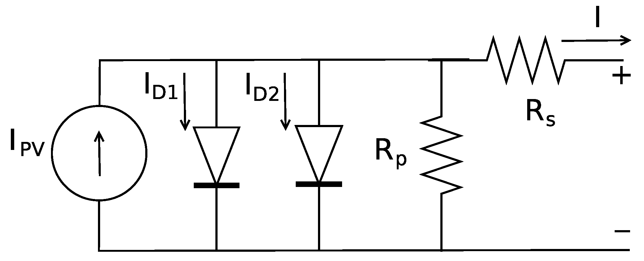
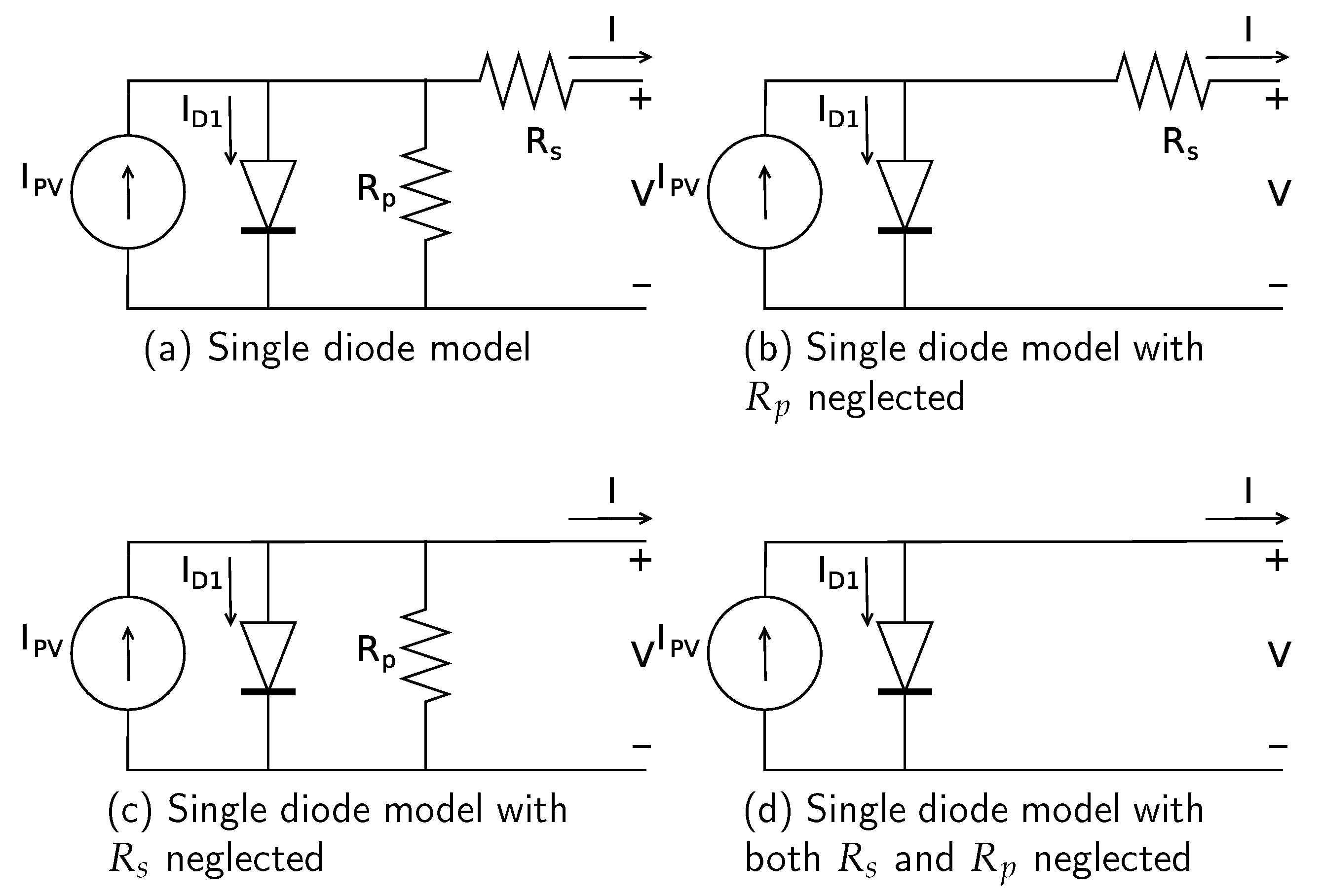
2.1. Models Description

In the following, we describe the five models we chose to implement on the emulation board. They are, to the best of our knowledge, representative of a wide range of state-of-the-art models with different features in terms of flexibility, accuracy, and computational requirements for their resolution [30].

• Two diodes model:

Figure 1 exemplifies a two diodes model with parallel and series resistance. It is currently considered, in literature, a model capable of accurately reproducing a broad spectrum of operating conditions [19,30]. It takes into consideration a series of aspects and features related to the production of energy from solar radiation, namely the following:

(1)

the classic PV effect, by means of current generator $I_{PV}$ and diode $D1$;

(2)

the effect of the recombination current in the depletion region, which particularly affects accuracy in the low-voltage region, by means of diode $D2$;

(3)

losses due to contact resistance (between silicon and electrodes surfaces) and materials resistance (silicon and electrodes metal), by means of series resistance $R_s$;

(4)

sensitivity to temperature variation and the effect of leakage current in the PN junction, by means of parallel resistance $R_p$.

The current–voltage relation of this equivalent circuit is described in Equation (1).

$$I=I_{PV}-I_{01}[\exp \left(\frac{q(V+I{R}_s)}{a_{1}kT}\right)-1]-I_{02}[\exp \left(\frac{q(V+I{R}_s)}{a_{2}kT}\right)-1]-\frac{V+I{R}_s}{R_p}$$

(1)

where $I_{PV}$ represents the PV current generated by the light incident on the panel; $I_{01}$ is the reverse saturation (or leakage) current associated to diode $D1$; $I_{02}$ is the reverse saturation (or leakage) current associated to diode $D2$; $a_1$ is the ideality factor of diode $D1$; $a_2$ is the ideality factor of diode $D2$; k is the Boltzmann constant (1.3806503 × 10⁻²³ J·K⁻¹); q is the electron charge (1.60217646 × 10⁻¹⁹ C); T is the temperature of the PN-junction. Introducing the so-called thermal voltage of the array ($V_t$) as $V_t=kT/q$ [19], Equation (1) can be rewritten as:

$$I=I_{PV}-I_{01}[\exp \left(\frac{(V+I{R}_s)}{V_t{a}_1}\right)-1]-I_{02}[\exp \left(\frac{(V+I{R}_s)}{V_t{a}_2}\right)-1]-\frac{V+I{R}_s}{R_p}$$

(2)

The model entails, however, the characterization of a significant number of parameters : $I_{PV}$, $I_{01}$, $I_{02}$, $a_1$, $a_2$, $R_s$, $R_p$.

• Single diode model:

In this model, shown in Figure 2a, the effect of the recombination current in the depletion region is not taken into account. Indeed, diode $D2$ is dropped, resulting in the current–voltage relationship described by Equation (3):

$$I=I_{PV}-I_0[\exp \left(\frac{V+I{R}_s}{V_{t}a}\right)-1]-\frac{V+I{R}_s}{R_p}$$

(3)

This model entails the evaluation of five parameters for its complete characterization: $I_{PV}$, $I_0$, a, $R_s$, $R_p$.

• Single diode model without parallel resistance:

Given the usually high values of $R_p$, some authors have proposed to neglect its effect (i.e., to consider $R_p=\infty$) to simplify the model [31,32,33,34,35,36]. The equivalent circuit of the single diode model without shunt resistance $R_p$ is depicted in Figure 2b. Equation (4) describes the resulting voltage–current relation:

$$I=I_{PV}-I_0[\exp \left(\frac{V+I{R}_s}{V_{t}a}\right)-1]$$

(4)

This model entails the evaluation of four parameters $I_{PV}$, $I_0$, a, $R_s$to complete the characterization.

• Single diode model without series resistance:

In the single diode model, the values of $R_s$ are typically low in most practical cases. Hence, its effect has been neglected in some works [37,38,39]. The resulting equivalent circuit is shown in Figure 2c, while the corresponding Several I–V relation is described by Equation (5).

$$I=I_{PV}-I_0[\exp \left(\frac{V}{V_{t}a}\right)-1]-\frac{V}{R_p}$$

(5)

There are also four model parameters to be derived in this case, namely: $I_{PV}$, $I_0$, a, and $R_p$.

• Single diode model without series and parallel resistance:

If neither the series resistance $R_s$, nor the parallel resistance $R_p$ are considered (i.e., $R_s=0$, $R_p=\infty$ in the single diode model), the model represented in Figure 2d is obtained. This is a very simplified model, whose behavior is described by Equation (6).

$$I=I_{PV}-I_0[\exp (\frac{V}{V_{t}a})-1]$$

(6)

On one hand, this is an ideal representation of a solar panel and, as such, it can be exploited for reasoning only on some basic, theoretical concepts related to PV arrays. On the other hand, it provides a useful comparison term to be included in our study, because of the low number of parameters to be obtained for its derivation ($I_{PV}$, $I_0$, a), and because of the simple structure of the Several I–V equation which allows significant savings in term of execution time. In light of these considerations, it can be taken as a lower bound for computational complexity.

In general, several approaches have been proposed for the derivation of model parameters. A coarse grain classification is usually done among analytical methods and curve fitting/optimization methods [30].

The former category of methods exploits information contained in components’ datasheets to derive a set of equations which are to be solved for parameters extraction. Given the nature of these equations (usually implicit, transcendental equations) and given that systems of equations relating them are often undetermined (i.e., there are more unknowns than equations) some heuristics are usually applied.

The latter type of solutions cast parameter extraction as a Several I–V curve fitting problem and solves it by means of optimization algorithms. The choice of a proper objective function and of the algorithm used to optimize it leads to various possible alternative methods.

While the focus of this article is on the model execution (in particular on the performance requirements of emulating a given model of small scale solar panels on embedded platforms), the interested reader can refer to a recent, comprehensive review of parameter extraction methods by Chin et al. [30].

2.2. Numerical Resolution Method

Once all parameters needed to characterize the model of the PV array are derived, emulation/simulation can be carried out. From the functional relationship among current and voltage expressed by Equations (1) and (3)–(6) and given a value of the current I (or of the voltage V), the corresponding value of voltage V (current I) can be derived from the nonlinear equations by means of numerical methods. We followed [19] and used the Newton–Raphson algorithm [40], a standard method to find roots of transcendental equations. In particular, if we formulate each of the Equations (1) and (3)–(6) as $f(V,I)=0$, the value of V can be obtained from a given I by finding the root of the modeling equation. At each iteration, the value of V is updated as follows:

$$V_{i+1}=V_i-\frac{f(V_i,I)}{\frac{\partial f(V_i,I)}{\partial V}}$$

(7)

until the stopping criterion $|V_{i+1}-V_i|<ϵ$ is met (ϵ is an implementation-dependent tolerance value).

To better highlight the computational requirements of the numerical algorithm, we report in the following both the nonlinear modeling function $f(V,I)$ and its partial derivative $\frac{\partial f(V_i,I)}{\partial V}$, for each investigated model.

• Two diodes model:

$$f(V,I)=I_{PV}-I_{01}[\exp \left(\frac{V+I{R}_s}{V_t{a}_1}\right)-1]-I_{02}[\exp \left(\frac{V+I{R}_{)}}{V_t{a}_2}\right)-1]-\frac{V+I{R}_s}{R_p}-I$$

(8)

$$\frac{\partial f(V_i,I)}{\partial V}=-\frac{I_{01}}{V_t{a}_1}\exp (\frac{V+I{R}_s}{V_t{a}_1})-\frac{I_{02}}{V_t{a}_2}\exp (\frac{V+I{R}_s}{V_t{a}_2})-\frac{1}{R_p}$$

(9)

From Equations (8) and (9), it follows that this model entails several arithmetic operations (e.g., four exponentials) to be carried out at run-time by the emulator, which leads to a potential computational bottleneck in real-time applications, as will be discussed in the section devoted to experimental results.

• Single diode model:

$$f(V,I)=I_{PV}-I_0[\exp \left(\frac{V+I{R}_s}{V_{t}a}\right)-1]-\frac{V+I{R}_s}{R_p}-I$$

(10)

$$\frac{\partial f(V_i,I)}{\partial V}=-\frac{I_0}{V_{t}a}\exp (\frac{V+I{R}_s}{V_{t}a})-\frac{1}{R_p}$$

(11)

In this case, the evaluation of Equations (10) and (11) requires a lower number of arithmetic operations (e.g., two exponentials instead of four at each iteration of the numerical algorithm) with regards to the two diodes model. This results in an expected improvement of computational performance.

• Single diode model without parallel resistance:

$$f(V,I)=I_{PV}-I_0[\exp \left(\frac{V+I{R}_s}{V_{t}a}\right)-1]-I$$

(12)

$$\frac{\partial f(V_i,I)}{\partial V}=-\frac{I_0}{V_{t}a}\exp (\frac{V+I{R}_s}{V_{t}a})$$

(13)

The execution time can be further lowered with respect to that of previous models because of the absence of terms $\frac{V+I{R}_s}{R_p}$ and $\frac{1}{R_p}$, which enables one to save three additions, a multiplication and two divisions at each of the iterations.

• Single diode model without series resistance:

$$f(V,I)=I_{PV}-I_0[\exp \left(\frac{V}{V_{t}a}\right)-1]-\frac{V}{R_p}-I$$

(14)

$$\frac{\partial f(V_i,I)}{\partial V}=-\frac{I_0}{V_{t}a}\exp (\frac{V}{V_{t}a})-\frac{1}{R_p}$$

(15)

Neglecting the series resistance enables one to save at each iteration three additions and three multiplications with regards to the single diode complete model. If we take, as a comparison term, the single diode model without parallel resistance, instead, performances are slightly worse: for the single diode model with $R_p=\infty$, we need, in fact, to compute two more additions and multiplications with regards to the single diode model with $R_s=0$ which, conversely, needs two more divisions and subtractions.

• Single diode model without series and parallel resistance:

$$f(V,I)=I_{PV}-I_0[\exp (\frac{V}{V_{t}a})-1]-I$$

(16)

$$\frac{\partial f(V_i,I)}{\partial V}=-\frac{I_0}{V_{t}a}\exp (\frac{V}{V_{t}a})$$

(17)

This simplest model enables, in principle, a further speedup in the implementation of the Newton–Raphson algorithm since it allows us to save two additions and two multiplications with regards to the single diode model without shunt resistance.

3. Tuning Models Complexity

To adequately tune the run-time complexity of the PV model (i.e., the resolution of the Several I–V curve) we propose a methodology which can be summarized as follows:

• For each model to be analyzed:

  -

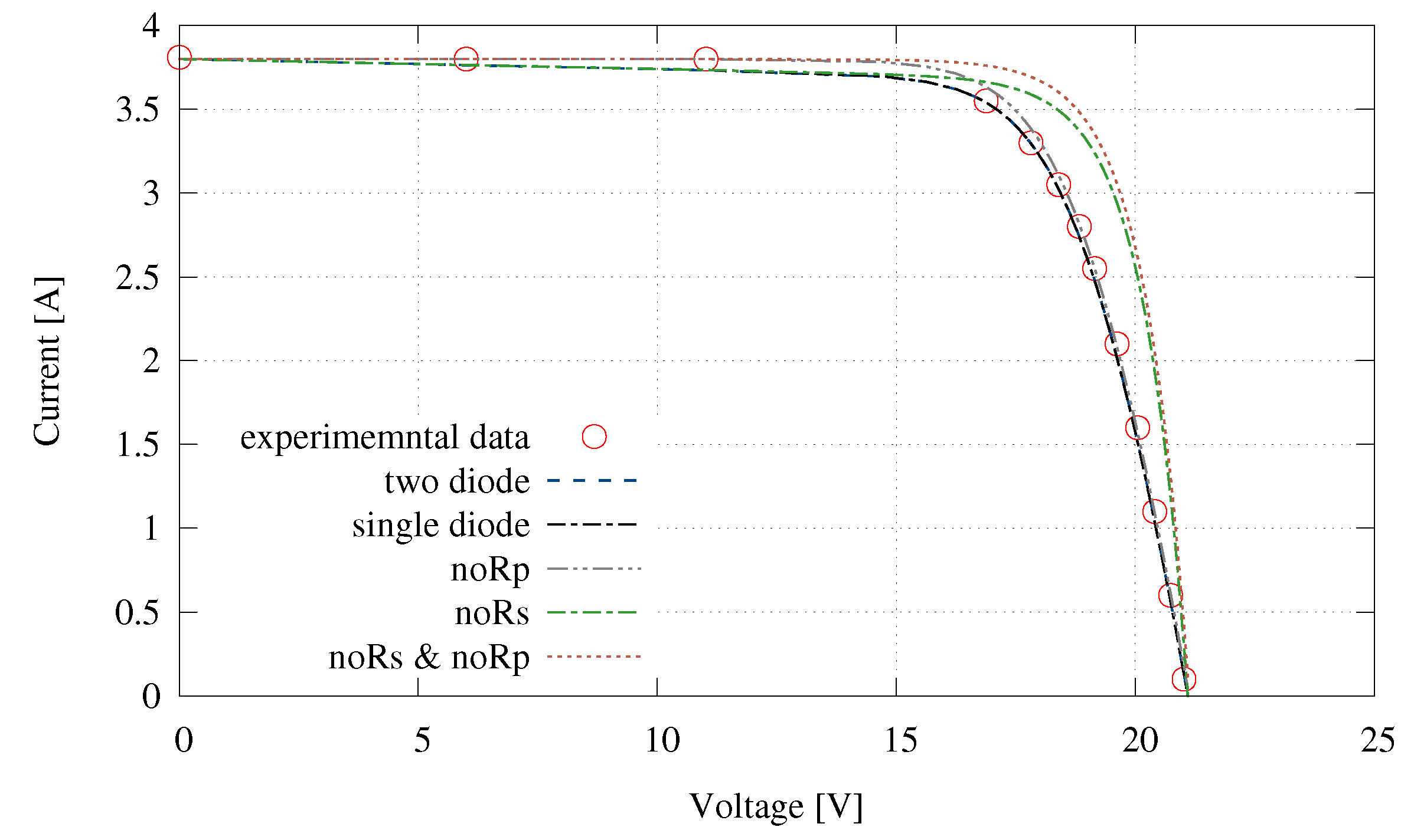
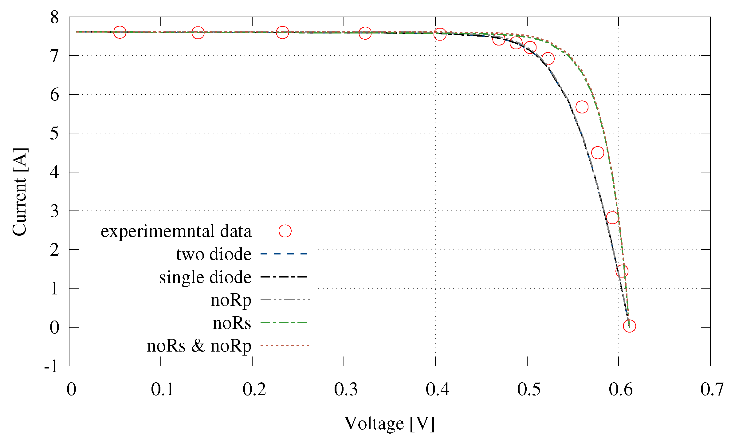
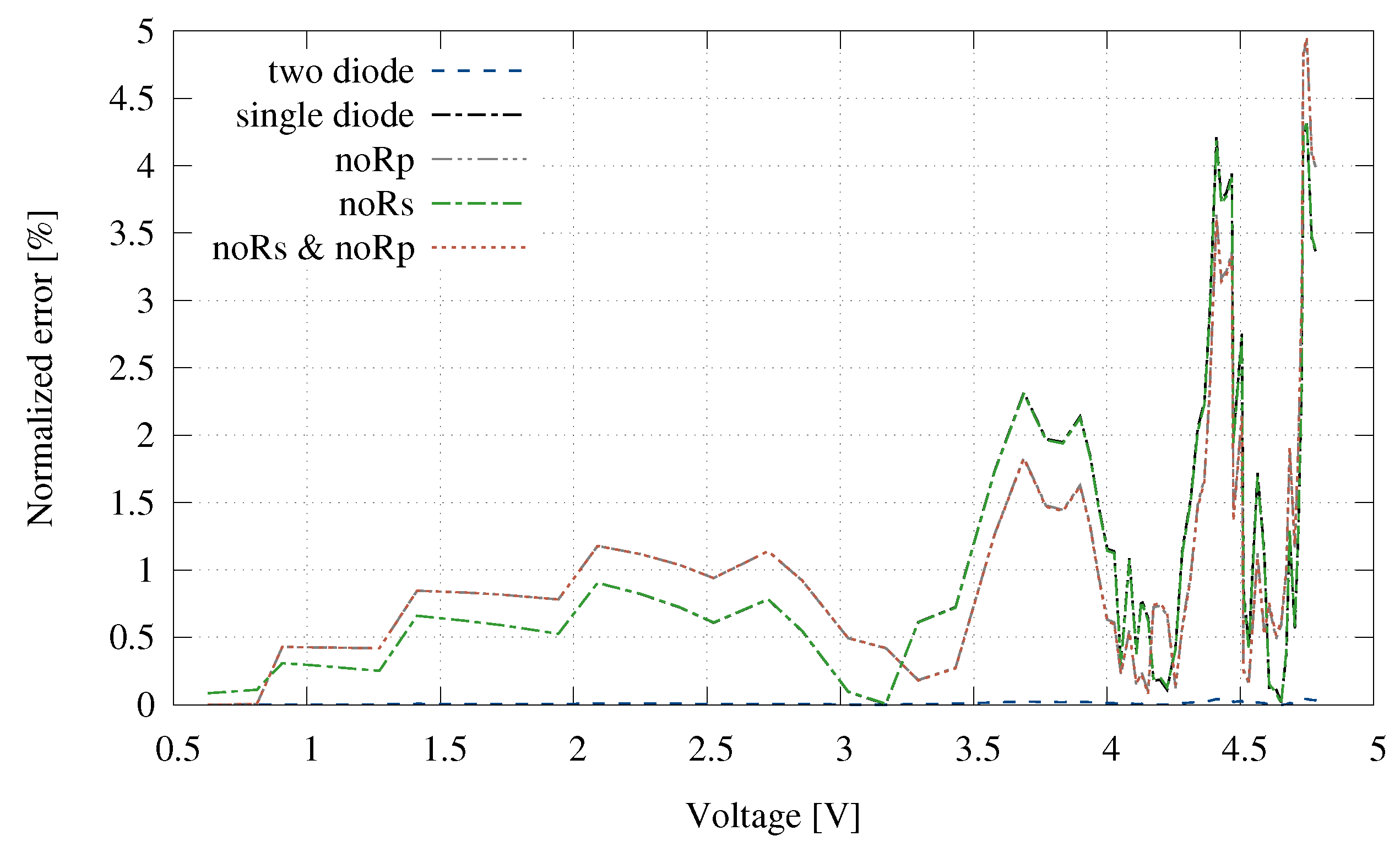
  the error achieved to reconstruct the Several I–V curve of a particular PV device by means of the model is measured;

  -

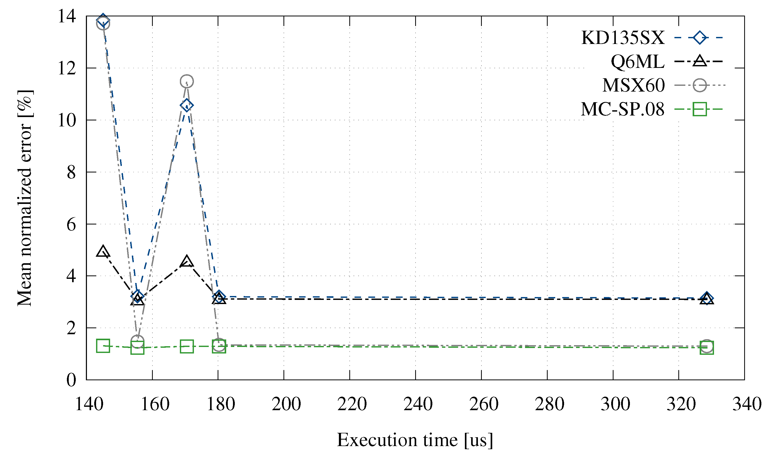
  the time required at run-time to resolve the model (i.e., to derive the voltage values to be applied by the emulation board from current values) is measured.

• The two empirically derived metrics are used to build a Pareto curve whose points correspond to the performance of different models when applied to a specific PV array. Indeed, the Pareto curve is a representation (commonly adopted in multi-objective optimization problems) of the achievable trade-offs between the metrics under study.
• The Pareto front is analyzed to obtain the optimal configuration (i.e., the most suitable model for that device).

For each of the five models described in Section 2, model parameters have been extracted, once and for all, following the method proposed by Villalva et al. [19]. Given the characterized model, the related Several I–V equation has been solved as described in Section 2.2 by means of the Newton–Raphson method [40] to obtain the run-time emulation working point. In particular, since in the embedded emulation platform, the current drained by the load is measured, the corresponding voltage values have been derived by numerical resolution. It is worth noticing that, conversely, many works related to PV array modeling usually assume the knowledge of voltage values to derive the corresponding current values.

The accuracy has been evaluated with respect to the capability of reproducing the current–voltage curve of real world devices. Four different commercially available PV arrays have been considered, resulting in 20 distinct emulation configurations.

The computational effort needed to obtain a working point (i.e., to derive, from a measured current, the voltage to be applied by the emulator) has been subsequently evaluated for each characterized model and for each array.

The information achieved from the characterization of the accuracy and latency of the system, allows us to draw some significant considerations. In particular, from the Pareto curve representing the two metrics, the model with the best performance trade-off can be selected.

Indeed, results highlight the reduced error levels attained by low-complexity models when applied to low-power, small form factor PV arrays. At the same time, low complexity models can be exploited to reduce the computational requirements imposed at run-time by the numerical resolution algorithm, thus making accurate, real-time emulation of energy harvesting sources on embedded systems possible.

4. Results and Discussion

To demonstrate the validity of the proposed approach, each of the five models described in Section 2 has been characterized and the related Several I–V equations have been solved by means of the numerical algorihms described in Section 2.2 which have been implemented in Matlab^® (MathWorks, Inc., Natick, MA, USA), for four different commercial PV arrays. The accuracy of each model has then been evaluated with respect to the capability of reproducing the Several I–V curve, extracted from the related datasheet, of the real world devices. It is worth noticing that this characterization is independent of the implementation on the embedded platform, since it aims at an evaluation of the error inherent to modelling assumptions.

Time needed to compute a single point of the Several I–V curve has been measured by running numerical solution of the models implemented to the embedded emulator platform presented in [17].

4.1. Experimental Set-Up

The four commercial PV arrays used in this work as case study are namely Solarex MSX60 (Solarex, Frederick, MD, USA) [41], Q.CELLS Q6ML-1600 (Q-Cells, Seoul, Korea) [42], Multicomp MC-SP-0.8 (Premier Farnell, Leeds, UK) [43], and Kyocera KD135SX (Kyocera, Kyoto, Japan) [44]. The selected PV arrays cover a wide spectrum of contexts of use. In particular, the MSX60 PV array is a 60 W high voltage module suitable for telecommunications systems, pumping and irrigation, and for general battery charging, while the Q6ML-1600 is a 3.78 W low voltage high current PV array capable of producing up to 7 A with a voltage of only 0.6 V. The Multicomp MC-SP-0.8 is a low size, high efficiency 0.8 W PV array producing up to 0.23 A at a maximum voltage of 4.5 V suitable for powering small embedded devices such as wireless sensor nodes, wearable and internet of things devices. Finally, the Kyocera KD135SX is a 135 W high voltage and high current PV array suitable for industrial and home installations.

The core of the embedded emulator platform, used to measure the time spent to compute a single point of the Several I–V curve, consists of the ATSAM4E16E microcontroller provided by Atmel Corporation (San Jose, CA, USA) which is based on a high-performance 32-bit ARM^® Cortex^®-M4 RISC processor ARM Holdings, Cambridge, UK running at a maximum speed of 120 MHz and features up to 128 Kbytes of RAM. From the analog point of view, the microcontroller is equipped with two 16-bit ADC and one 12-bit DAC providing two separate channels.

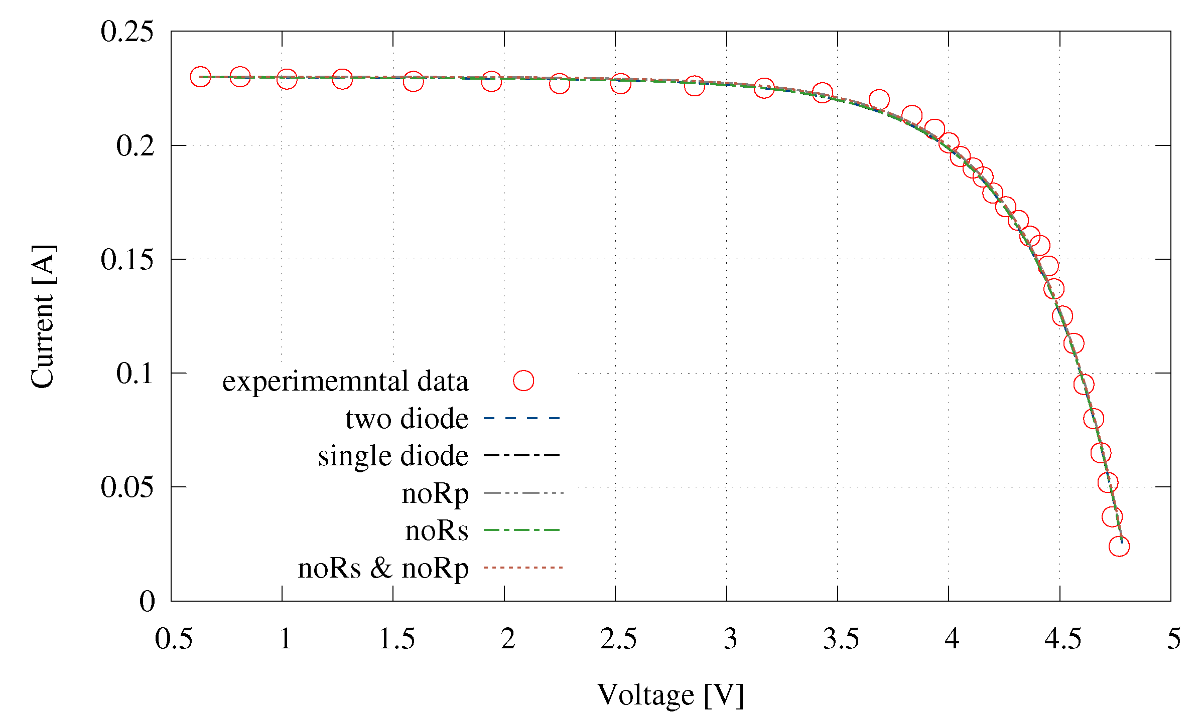
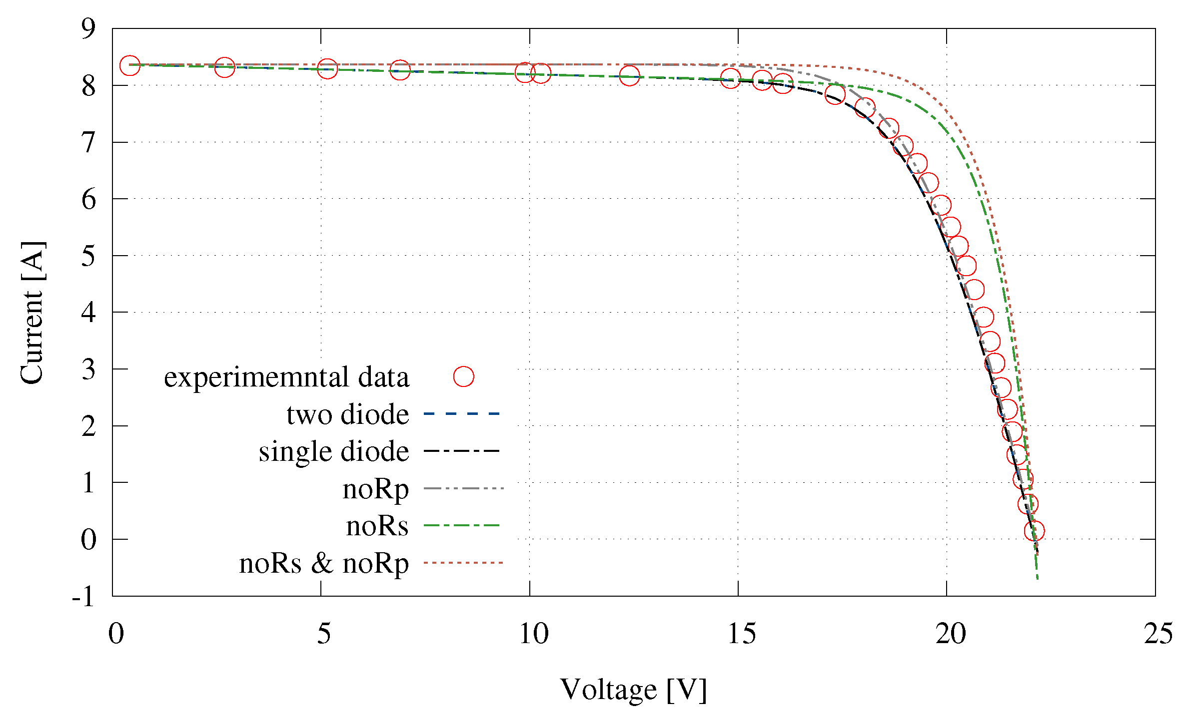
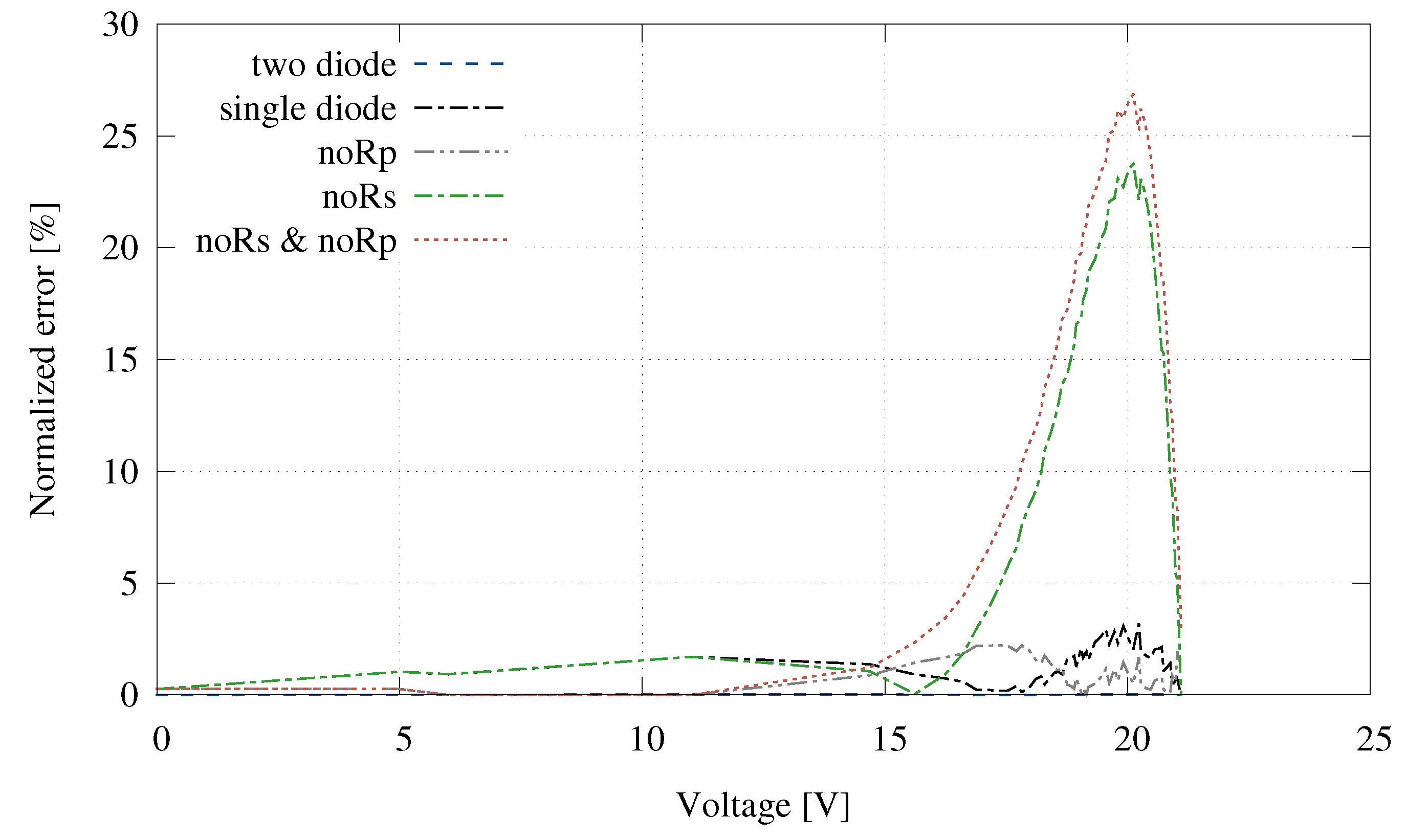
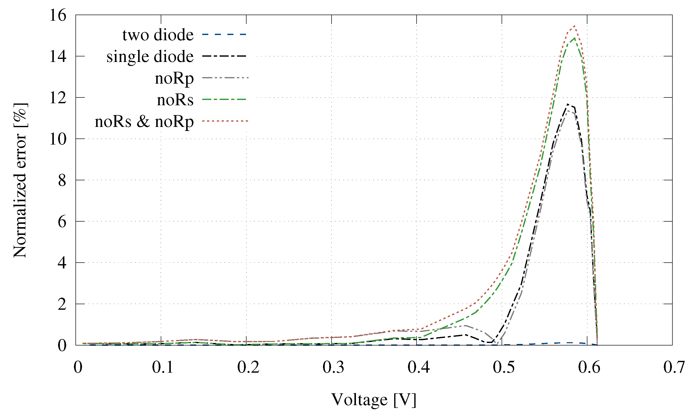
4.2. Experimental Results

The experimental (I, V) points were extracted from the manufacturer’s datasheet of each panel and compared with the simulated data obtained while varying the complexity of the PV model.

Table 1. Parameters of the simulation models.

Parameter	MC-SP.08	MSX60	Q6ML	KD135SX
$I_{SC}$ (A)	0.23	3.8	7.61	8.37
$V_{OC}$ (V)	4.83	21.1	0.611	22.1
$I_{mp}$ (A)	0.21	3.5	7.11	7.63
$V_{mp}$ (V)	3.85	17.1	0.51	17.7
$I_{D1}$ = $I_{D2}$ (A)	1.8 × 10−6	4.5 × 10−10	3.4 × 10−10	3.4 × 10−10
$I_{PV}$ (A)	0.23	3.81	7.61	8.4
$a_1$	1.0	1.0	1.0	1.0
$a_2$	3.5	1.5	2.5	4.5
$R_p$ (Ω)	3320	166	13	56
$R_s$ (Ω)	0.02	0.37	0.05	0.22

shows both the parameters extracted from the datasheet and obtained during model adjustment which are used in the PV array simulations. Notice that for the two diodes, model $I_{D1}$ and $I_{D2}$ are set to be equal in magnitude and they have been calculated at standard temperature conditions using Equation (7) reported in the work of Villalva et al. [19]. The diffusion current $a_1$, in accordance with Shockley’s diffusion theory, has been set equal to unit, while the value of $a_2$ has been chosen by means of numerical fitting according to the methodology adopted in previous work [20,45]: the value has been iteratively adjusted in order to find the best match between the model and the experimental Several I–V curve.

The adjusted models have then been solved to calculate the Several I–V curve starting from a set of values of V, (the tolerance value ϵ has been set to 10⁻⁴). Figure 3, Figure 4, Figure 5 and Figure 6 show the Several I–V curves obtained by solving the set of models with decreasing complexity for the four reference PV arrays compared with the experimental data extracted by the datasheet. Datasheet values are shown by means of red circles while the modeled Several I–V curves are represented by the dotted lines. Notice that, for the sake of readability, the (I, V) pair values from the datasheets have been downsampled in the plot, but they have been entirely used to derive the results described below.

The results related to the Solarex MSX60 PV module, presented in Figure 3, show that the two diode and the single diode models (the blue and black dotted lines) follow the experimental data in an almost perfect way while the single diode model without the parallel resistance (the gray dotted line) introduces a non negligible approximation error in high current conditions. On the other hand, removing the series resistance (the green dotted line) causes a great mismatch between the model and the ground truth datasheets data. The last model simplification (the red dotted line) which remove both the series and the parallel resistance results, as expected, in an even larger approximation error. Similar considerations can be made for the Q.CELLS Q6ML-1600 and for the Kyocera KD135SX PV modules (Figure 4 and Figure 6) while particular attention must be given to the results obtained while modeling the Multicomp MC-SP-0.8 PV module (Figure 5). In fact, in this case, no appreciable mismatches can be highlighted between the models and the experimental data while reducing the model complexity. The limited current and voltage produced by the MC-SP-0.8 PV module lead to a very low impact on the resulting accuracy of the more complicated modeling strategies currently adopted in literature. Thus, new trade-offs between complexity and accuracy can be evaluated while modeling low power PV arrays suitable for powering embedded devices.

Figure 7, Figure 8, Figure 9 and Figure 10 show the normalized error calculated while reconstructing the Several I–V curves of Figure 3, Figure 4, Figure 5 and Figure 6. Notice that, to directly compare different PV array modules characterized by different dynamic ranges, the measured errors have been normalized with respect to the $I_{sc}$. As expected, the higher the $I_{sc}$ provided by the PV array, the higher the approximation error measured while reducing the model complexity. For instance, KD135SX and MSX60, which are high current modules, show a maximum normalized error around 30% while removing the series, or both series and parallel resistances from the model. On the other hand, for a medium-current PV array such as the Q6ML-1600, the maximum normalized error never exceeds 16% and for the low-voltage/low-current MC-SP-0.8 PV array, the maximum measured error obtained while removing both the series and the parallel resistances is extremely reduced and it remains always under a threshold of about 5%.

Figure 7, Figure 8, Figure 9 and Figure 10 also provide an overview of the error distribution along the operating voltage range. While in the low-voltage/high-current region, the measured error always remains under an appreciable level, in the region going from the maximum power point to the open circuit voltage, the measured error reaches the highest values for the simplest model. In the case of the low-voltage/low-current MC-SP-0.8 PV array, the error distribution along the voltage (Figure 9) does not show considerable growth focused on the region following the maximum power point, both in the case of more complex models and in the case of simpler ones.

Table 2. Mean normalized error (MNE) and execution times obtained while tuning the model complexity for different PV Arrays.

Model	MC-SP.08	MSX60	Q6ML	KD135SX	Execution Time (μs)
	MNE (%)
Complete	1.24	1.30	3.10	3.15	328.5
Single diode	1.29	1.35	3.10	3.15	180.3
No $R_p$	1.25	1.47	3.11	3.65	155.5
No $R_s$	1.29	11.49	4.55	10.57	170.5
No $R_p$ & No $R_s$	1.30	13.72	4.93	13.85	145.1

summarize the models’ performance by reporting the mean normalized error (MNE), which is the average normalized error calculated along the whole voltage range of the Several I–V curve, obtained while simulating the PV array with the models described in Section 2.1. An average execution time for each model has also been reported. The execution time has been calculated by porting and executing the numerical solutions of each model, described in Section 2.2, to the target embedded emulator presented in [17]. The reported execution time is an average value measured while the emulator was calculating the corresponding values of V for 100 different values of I. As expected, the measured execution times reflect the observations reported in Section 2.2 highlighting the strong contribution of the solution of the four exponentials of the complete models. In fact, in this case, the execution time almost doubles those obtained with the other models, which need to compute only two exponentials to be solved.

Figure 11 shows the Pareto curve of the execution time vs. the MNE, obtained for each PV array. The orthogonal red dotted lines define a region in which the PV array can be emulated using the embedded hardware without impairing the emulation performance. In fact, in this region, the MNE is always lower than 5% (a threshold set to ensure reasonably accurate emulation) and the execution time never exceeds the hardware emulator latency, which has been estimated to be about 172 μs on average (see [17]). Thus, each point pair (model configuration, PV array) which falls inside the region can be suitably emulated by the embedded device. For instance, the KD135SX PV array can only be emulated in the configuration with a single diode without parallel resistance while all other configurations fall outside of the region. On the other hand, a low-current and low-voltage PV array such as the MC-SP.08, which is a module traditionally used to power wireless sensor nodes, shows a Pareto curve which is almost a horizontal line so that all three of the simplest model configurations can be used to emulate the PV array.

5. Conclusions

The design of energy efficient networked embedded systems is severely hampered by the lack of flexible frameworks for experimentally testing new solutions. This task is usually achieved either by simulation or by direct implementation on testbeds. While simulation provides the opportunity to explore in a reproducible fashion large portions of the design space, it inherently approximates many aspects of real-world operating conditions. Conversely, testbeds represent a convenient alternative to carry out realistic experiments, at the price of high costs and reduced flexibility and reproducibility.

This scenario is further complicated if energy harvesting and workload variability are taken into consideration. Indeed, the dynamics of energy harvesting sources are particularly difficult to predict and, at the same time, load impedances could frequently change, for instance according to different dynamic power management states applied to the devices. Emulation is considered a valuable option which enables reliable reproduction of many different energy sources (e.g., harvesting devices) within a repeatable and controlled set up. However, in order to cope with real-time requirements when dealing with resource-constrained embedded devices, the complexity of the models implemented on the emulation board should be carefully evaluated.

In this paper, we presented a novel methodology aimed at tuning the complexity of PV array models executed by embedded emulators. The proposed approach allows one to explore the trade off between the accuracy and latency of the emulation process, thus providing a flexible resource for system design of real-time compatible, low-cost embedded emulation boards. Experimental results on a representative set of commercially available PV arrays demonstrate the effectiveness of the introduced technique. A remarkable conclusion obtained is that low-power PV arrays with small form factor and low voltage–current levels can be emulated on embedded platforms to meet real-time constraints without introducing significant errors.

References

1. Kansal, A.; Hsu, J.; Zahedi, S.; Srivastava, M.B. Power management in energy harvesting sensor networks. ACM Trans. Embed. Comput. Syst. 2007, 6. [Google Scholar] [CrossRef]
2. Jeong, J.; Culler, D. A practical theory of micro-solar power sensor networks. ACM Trans. Sens. Netw. 2012, 9. [Google Scholar] [CrossRef]
3. Jeong, J.; Culler, D. Predicting the long-term behavior of a micro-solar power system. ACM Trans. Embed. Comput. Syst. 2012, 11. [Google Scholar] [CrossRef]
4. Bogliolo, A.; Freschi, V.; Lattanzi, E.; Murphy, A.L.; Raza, U. Towards a true energetically sustainable WSN: A case study with prediction-based data collection and a wake-up receiver. In Proceedings of 9th IEEE International Symposium on Industrial Embedded Systems (SIES 2014), Pisa, Italy, 18–20 June 2014; pp. 21–28.
5. Bogliolo, A.; Lattanzi, E.; Freschi, V. Idleness as a resource in energy-neutral WSNs. In Proceedings of the 2013 1st International Workshop on Energy Neutral Sensing Systems (ENSSys), Rome, Italy, 14 November 2013; ACM: New York, NY, USA, 2013; pp. 1–6. [Google Scholar]
6. Raza, U.; Bogliolo, A.; Freschi, V.; Lattanzi, E.; Murphy, A.L. A two-prong approach to energy-efficient WSNs: Wake-up receivers plus dedicated, model-based sensing. Ad Hoc Netw. 2016, 45, 1–12. [Google Scholar] [CrossRef]
7. Chou, P.H.; Park, C.; Park, J.; Pham, K.; Liu, J. B#: A battery emulator and power profiling instrument. In Proceedings of the 2003 International Symposium on Low Power Electronics and Design, Seoul, Korea, 25–27 August 2003; pp. 288–293.
8. Li, D.J.; Chou, P.H. Maximizing efficiency of solar-powered systems by load matching. In Proceedings of the 2004 International Symposium on Low Power Electronics and Design (ISLPED), Newport Beach, CA, USA, 9–11 August 2004; pp. 162–167.
9. Atia, Y.; Zahran, M.; Al-Hossain, A. Solar cell emulator and solar cell characteristics measurements in dark and illuminated conditions. WSEAS Trans. Syst. Control 2011, 6, 125–135. [Google Scholar]
10. Lee, W.; Kim, Y.; Wang, Y.; Chang, N.; Pedram, M.; Han, S. Versatile high-fidelity photovoltaic module emulation system. In Proceedings of the International Symposium on Low Power Electronics and Design, Fukuoka, Japan, 1–3 August 2011; pp. 91–96.
11. Thale, S.; Wandhare, R.; Agarwal, V. A novel low cost portable integrated solar PV, fuel cell and battery emulator with fast tracking algorithm. In Proceedings of the 2014 IEEE 40th Photovoltaic Specialist Conference (PVSC), Denver, CO, USA, 8–3 June 2014; pp. 3138–3143.
12. Chen, C.C.; Chang, H.C.; Kuo, C.C.; Lin, C.C. Programmable energy source emulator for photovoltaic panels considering partial shadow effect. Energy 2013, 54, 174–183. [Google Scholar] [CrossRef]
13. González-Medina, R.; Patrao, I.; Garcerá, G.; Figueres, E. A low-cost photovoltaic emulator for static and dynamic evaluation of photovoltaic power converters and facilities. Prog. Photovolt. Res. Appl. 2014, 22, 227–241. [Google Scholar] [CrossRef]
14. Bobovych, S.; Banerjee, N.; Robucci, R.; Parkerson, J.P.; Schmandt, J.; Patel, C. SunaPlayer. In Proceedings of the 2015 14th International Conference on Information Processing in Sensor Networks (IPSN), Seattle, WA, USA, 13–16 April 2015; ACM Press: New York, NY, USA, 2015; pp. 59–70. [Google Scholar]
15. Zhang, H.; Salajegheh, M.; Fu, K.; Sorber, J. Ekho: Bridging the gap between simulation and reality in tiny energy-harvesting sensors. In Proceedings of the 2011 4th Workshop on Power-Aware Computing and Systems (HotPower), Cascasis, Portugal, 23 October 2011; pp. 1–5.
16. Hester, J.; Scott, T.; Sorber, J. Ekho: Realistic and repeatable experimentation for tiny energy-harvesting sensors. In Proceedings of the 2014 12th ACM Conference on Embedded Network Sensor Systems (SenSys), Memphis, TN, USA, 3–6 November 2014; pp. 1–15.
17. Lattanzi, E.; Freschi, V.; Dromedari, M.; Lorello, L.S.; Peruzzini, R.; Bogliolo, A. A fast and accurate energy source emulator for wireless sensor networks. EURASIP J. Embed. Syst. 2016, 2016. [Google Scholar] [CrossRef]
18. Vergura, S. A complete and simplified datasheet-based model of PV cells in variable environmental conditions for circuit simulation. Energies 2016, 9, 326. [Google Scholar] [CrossRef]
19. Villalva, M.G.; Gazoli, J.R.; Filho, E.R. Comprehensive approach to modeling and simulation of photovoltaic arrays. IEEE Trans. Power Electron. 2009, 24, 1198–1208. [Google Scholar] [CrossRef]
20. Ishaque, K.; Salam, Z.; Taheri, H. Simple, fast and accurate two-diode model for photovoltaic modules. Sol. Energy Mater. Sol. Cells 2011, 95, 586–594. [Google Scholar] [CrossRef]
21. Ishaque, K.; Salam, Z.; Syafaruddin. A comprehensive MATLAB Simulink PV system simulator with partial shading capability based on two-diode model. Sol. Energy 2011, 85, 2217–2227. [Google Scholar] [CrossRef]
22. Ishaque, K.; Salam, Z.; Taheri, H.; Syafaruddin. Modeling and simulation of photovoltaic (PV) system during partial shading based on a two-diode model. Simul. Model. Pract. Theory 2011, 19, 1613–1626. [Google Scholar] [CrossRef]
23. Seyedmahmoudian, M.; Mekhilef, S.; Rahmani, R.; Yusof, R.; Renani, E.T. Analytical modeling of partially shaded photovoltaic systems. Energies 2013, 6, 128–144. [Google Scholar] [CrossRef] [Green Version]
24. Di Vincenzo, M.C.; Infield, D. Detailed PV array model for non-uniform irradiance and its validation against experimental data. Sol. Energy 2013, 97, 314–331. [Google Scholar] [CrossRef]
25. Park, J.Y.; Choi, S.J. A novel datasheet-based parameter extraction method for a single-diode photovoltaic array model. Sol. Energy 2015, 122, 1235–1244. [Google Scholar] [CrossRef]
26. Bastidas, J.D.; Franco, E.; Petrone, G.; Ramos-Paja, C.A.; Spagnuolo, G. A model of photovoltaic fields in mismatching conditions featuring an improved calculation speed. Electr. Power Syst. Res. 2013, 96, 81–90. [Google Scholar] [CrossRef]
27. Ciulla, G.; Lo Brano, V.; Di Dio, V.; Cipriani, G. A comparison of different one-diode models for the representation of I-V characteristic of a PV cell. Renew. Sustain. Energy Rev. 2014, 32, 684–696. [Google Scholar] [CrossRef]
28. Li, Y.; Shi, R. An intelligent solar energy-harvesting system for wireless sensor networks. EURASIP J. Wirel. Commun. Netw. 2015, 2015. [Google Scholar] [CrossRef]
29. Brunelli, D.; Dondi, D.; Bertacchini, A.; Larcher, L.; Pavan, P.; Benini, L. Photovoltaic scavenging systems: Modeling and optimization. Microelectron. J. 2009, 40, 1337–1344. [Google Scholar] [CrossRef]
30. Chin, V.J.; Salam, Z.; Ishaque, K. Cell modelling and model parameters estimation techniques for photovoltaic simulator application: A review. Appl. Energy 2015, 154, 500–519. [Google Scholar] [CrossRef]
31. Khouzam, K.; Ly, C.; Koh, C.K.; Ng, P.Y. Simulation and real-time modelling of space photovoltaic systems. In Proceedings of the Conference Record of the Twenty Fourth Photovoltaic Energy Conversion and 1994 IEEE First World Conference on IEEE Photovoltaic Specialists Conference, Waikoloa, HI, USA, 5–9 December 1994; Volume 2, pp. 2038–2041.
32. Kuo, Y.C.; Liang, T.J.; Chen, J.F. Novel maximum-power-point-tracking controller for photovoltaic energy conversion system. IEEE Trans. Ind. Electron. 2001, 48, 594–601. [Google Scholar]
33. Matagne, E.; Chenni, R.; El Bachtiri, R. A photovoltaic cell model based on nominal data only. In Proceedings of the 2007 International Conference on Power Engineering, Energy and Electrical Drives, Setubal, Portugal, 12–14 April 2007; pp. 562–565.
34. Walker, G. Evaluating MPPT converter topologies using a MATLAB PV model. J. Electr. Electron. Eng. 2001, 21, 49–56. [Google Scholar]
35. Xiao, W.; Dunford, W.G.; Capel, A. A novel modeling method for photovoltaic cells. In Proceedings of the 2004 IEEE 35th Annual Power Electronics Specialists Conference (PESC), Aachen, Germany, 20–25 June 2004; Volume 3, pp. 1950–1956.
36. Yusof, Y.; Sayuti, S.H.; Latif, M.A.; Wanik, M.Z.C. Modeling and simulation of maximum power point tracker for photovoltaic system. In Proceedings of the 2004 National Power and Energy Conference (PECon), Kuala Lumpur, Malaysia, 29–30 November 2004; pp. 88–93.
37. Glass, M.C. Improved solar array power point model with SPICE realization. In Proceedings of the 31st Intersociety Energy Conversion Engineering Conference (IECEC 96), Washington, DC, USA, 11–16 August 1996; Volume 1, pp. 286–291.
38. Kajihara, A.; Harakawa, A. Model of photovoltaic cell circuits under partial shading. In Proceedings of the 2005 IEEE International Conference on Industrial Technology, Hong Kong, China, 14–17 December 2005; pp. 866–870.
39. Benavides, N.D.; Chapman, P.L. Modeling the effect of voltage ripple on the power output of photovoltaic modules. IEEE Trans. Ind. Electron. 2008, 55, 2638–2643. [Google Scholar] [CrossRef]
40. Quaschning, V.; Hanitsch, R. Numerical simulation of current-voltage characteristics of photovoltaic systems with shaded solar cells. Sol. Energy 1996, 56, 513–520. [Google Scholar] [CrossRef]
41. Solarex. MSX-60 and MSX-64 Photovoltaic Modules. Available online: http://www.solarelectricsupply.com/media/custom/upload/Solarex-MSX64.pdf (accessed on 12 October 2016).
42. Q.Cells. Hanwha Q Cells Solar Panels. Available online: https://www.q-cells.com/products/solar-panels.html (accessed on 12 October 2016).
43. Multicomp. MC-SP0.8-NF-GCS. Available online: http://www.farnell.com/datasheets/925851.pdf (accessed on 12 October 2016).
44. Kyocera. KD135SX-UFU. Available online: http://pdf.wholesalesolar.com/module%20pdf%20folder/KD135SX_UPU.pdf (accessed on 12 October 2016).
45. Sah, C.T. Fundamentals of Solid-State Electronics; World Scientific: Singapore, 1991. [Google Scholar]
Figure 1. The two diodes equivalent circuit of a photovoltaic (PV) array.
Energies 10 00278 g001
Figure 2. PV array models with decreasing complexity.
Energies 10 00278 g002
Figure 3. Results of model tuning for Solarex MSX60 PV module.
Energies 10 00278 g003
Figure 4. Results of model tuning for Q.CELLS Q6ML-1600 PV module.
Energies 10 00278 g004
Figure 5. Results of model tuning for Multicomp MC-SP-0.8 PV module.
Energies 10 00278 g005
Figure 6. Results of model tuning for Kyocera KD135SX PV module.
Energies 10 00278 g006
Figure 7. Normalized error obtained while reconstructing the Several IV curve for Solarex MSX60 PV module with different model complexity.
Energies 10 00278 g007
Figure 8. Normalized error obtained while reconstructing the Several IV curve for Q.CELLS Q6ML-1600 PV module with different model complexity.
Energies 10 00278 g008
Figure 9. Normalized error obtained while reconstructing the Several IV curve for Multicomp MC-SP-0.8 PV module with different model complexity.
Energies 10 00278 g009
Figure 10. Normalized error obtained while reconstructing the Several IV curve for Kyocera KD135SX PV module with different model complexity.
Energies 10 00278 g010
Figure 11. Execution times vs. MNE for each PV array.
Energies 10 00278 g011