Article

A New Model for Estimating the Diffuse Fraction of Solar Irradiance for Photovoltaic System Simulations

by
Martin Hofmann
1,2,* and
Gunther Seckmeyer
2
1
Valentin Software GmbH, Stralauer Platz 34, 10243 Berlin, Germany
2
Leibniz Universität Hannover, Institute for Meteorology and Climatology, Herrenhäuser Straße 2, 30419 Hannover, Germany
*
Author to whom correspondence should be addressed.
Energies 2017, 10(2), 248; https://doi.org/10.3390/en10020248
Submission received: 21 December 2016 / Revised: 6 February 2017 / Accepted: 13 February 2017 / Published: 18 February 2017

Abstract

:
We present a new model for the calculation of the diffuse fraction of the global solar irradiance for solar system simulations. The importance of an accurate estimation of the horizontal diffuse irradiance is highlighted by findings that an inaccurately calculated diffuse irradiance can lead to significant over- or underestimations in the annual energy yield of a photovoltaic (PV) system by as much as 8%. Our model utilizes a time series of global irradiance in one-minute resolution and geographical information as input. The model is validated by measurement data of 28 geographically and climatologically diverse locations worldwide with one year of one-minute data each, taken from the Baseline Surface Radiation Network (BSRN). We show that on average the mean absolute deviation of the modelled and the measured diffuse irradiance is reduced from about 12% to about 6% compared to three reference models. The maximum deviation is less than 20%. In more than 80% of the test cases, the deviation is smaller 10%. The root mean squared error (RMSE) of the calculated diffuse fractions is reduced by about 18%.

1. Introduction

Adapting the common terminology in energy meteorology to differentiate between the power and energy of the solar radiation, the word ‘irradiance’ is used in this work to denote the instantaneous solar power per square meter in W/m², whereas the word ‘irradiation’ refers to the integral of the irradiance over time, thus denoting the energy of the solar radiation in Ws/m² or kWh/m² [1].
In photovoltaic (PV) system simulations, the global horizontal irradiance and the ambient temperature are the two most important inputs in order to determine the PV system’s energy output. The global horizontal irradiance is split up in its direct and diffuse components. These components are then separately translated to a tilted plane if the PV system in question has a module orientation that differs from the horizontal plane. In simple terms the global irradiance incident on a tilted module is then calculated as the sum of the direct and the diffuse irradiance on the tilted plane.
The model for estimating the diffuse fraction of the global horizontal irradiance is hence the first element in a chain of models that is necessary to simulate the electrical output of a PV system. As such, it has strong influence on the final output of the simulation, which is demonstrated by the following comparative simulations for two locations: Lindenberg, Germany and Gobabeb, Namibia. The analysed PV system is a standard 8 kWp (kilo Watt peak) grid connected system, the simulation is conducted in one-minute resolution with measurement data from the Baseline Surface Radiation Network (BSRN) [2].
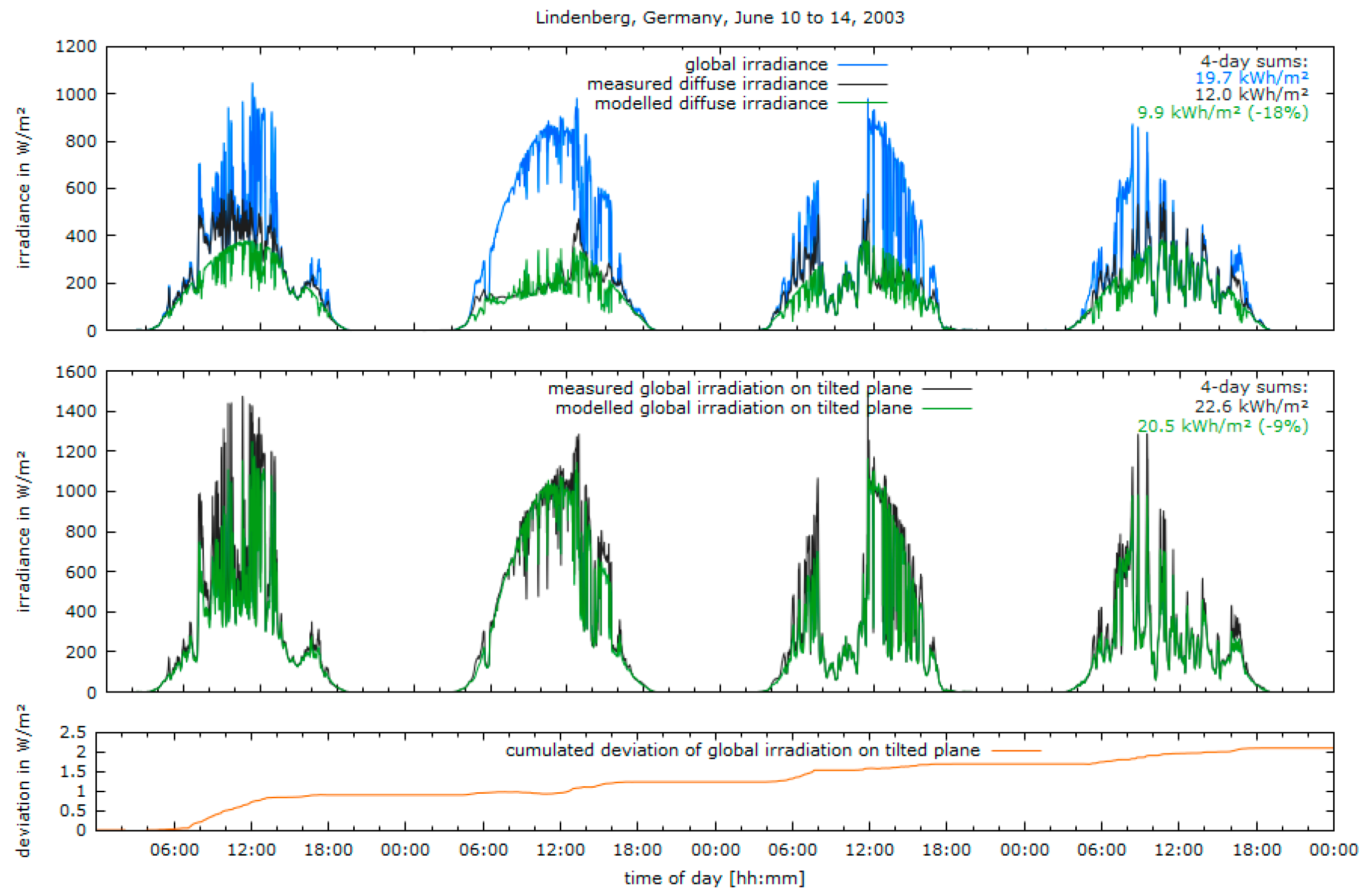
During the four exemplary days in June in Lindenberg, Germany, chosen for Figure 1, the model used for this comparison (reduced version of Reindl et al. [3]) underestimates the diffuse irradiance by 18%. In the next step of the simulation, the global irradiance on the tilted plane is calculated. In this case the modules are facing south and are elevated by 30° from the horizontal. The model applied for this step is from Hay and Davies [4]. When using the modelled horizontal diffuse irradiance, the resulting global irradiance on the modules is still 9% lower than using the measured horizontal diffuse irradiance.
The rest of the PV system model chain is then simulated with the help of the simulation core of PV software provider Valentin Software (Berlin, Germany) [5]. Table 1 lists the results of the comparison.
During these four days, the total PV energy yield would be 65.6 kWh when using the measured horizontal diffuse irradiance values. With the diffuse irradiance modelled by Reindl et al. [3], the total PV energy yield is only 60.2 kWh—an underestimation of 8.3%. The comparison was also conducted for the whole year 2003 in Lindenberg, where the annual deviation of the modelled diffuse irradiance is −7.2%, leading to a deviation of the annual PV energy output of −2.7%.
The second half of Table 1 lists the results of the same comparison that was conducted for the location of Gobabeb in Namibia, for the year 2014. Here, the deviation of the annual diffuse irradiation is as high as 42% which leads to an overestimation of the global irradiation of the module surface of 8.3% and to an overestimation of the annual PV energy yield of 7.6%.
These examples highlight the importance of a more accurate estimation of the horizontal diffuse irradiance. An inaccurately calculated diffuse irradiance can lead to significant over- or underestimations in the annual energy yield of a PV system. This is especially relevant in the price sensitive market of PVs, where only few percent more or less of PV energy output can render a project possible or uneconomical [6].

2. Measurement Data and Methodology

In the following section the measurement data and the methodology used in this contribution are presented.

2.1. Data basis (Baseline Surface Radiation Network)

As a source of high quality measurement data the data base of the BSRN is used [2]. The BSRN comprises 59 stations worldwide, 44 of which provide one-minute measurements of global horizontal and diffuse horizontal irradiance. The time range of the measurements starts in 1992 for the first stations and is still running until now. For this study the following criteria were applied for selecting the datasets:
  • High annual completeness of one-minute measurements of global and diffuse irradiance;
  • Between 60° North and −60° South;
  • No leap years.
Table 2 gives an overview of the locations and years that were used for validation. In total, 28 locations with one year of measurement each were selected. The datasets feature a high geographic and climatological diversity. The last column of the table lists the annual completeness of the measurements (ACM) in %. The validation datasets comprise more than seven million data points (nights omitted) on which the following analysis is based.

2.2. Description of Quantities and Models

For the calculation of the position of the sun, the solar position algorithm provided by the National Renewable Energy Laboratory (NREL; Golden, CO, USA) is used [8]. The clear sky irradiance E clear is calculated on the basis of an adaption of the approach of Bourges [9]:
E clear = 0.78 E ext sin ( γ S ) 1.15
where γ S is the elevation of the Sun and E ext is the extra-terrestrial irradiance. The extra-terrestrial irradiance was calculated using Maxwell’s approach [10]. In 2014 this formula was identified as the most accurate for another subset of BSRN data by Hofmann et al. [11]. The clearness index k t is the fraction of the measured global irradiance to the clear sky irradiance:
k t = E global ,   measured E clear
In the models for calculating the diffuse fraction of the global irradiance that are presented in Section 2.3 a simpler approach of calculating the clear sky index is used:
E clear = E ext sin ( γ S )
This causes the k t value at clear sky to be around 0.8 instead of 1 in the existing models. For the comparison of the results in Section 4, the calculation of the clearness index occurs according to the respective model description.
All PV system simulations are conducted using the simulation core of PV*SOL, a commercial PV system planning and simulation software by Valentin Software. More information about the models that are relied on in the simulation core can be found at PV*SOL [5].

2.3. Presentation of Existing Models

For the estimation of the diffuse fraction of the global horizontal irradiance, several algorithms were developed in the past. Most of them can be categorized as models with one or two parameters as input. The one-parameter models feature a simple dependency of the diffuse fraction ( d f ) on the clearness index ( k t ), cf. Figure 2.
These models typically define three functions for different ranges of k t . These k t ranges can be more or less referred to as different cloud situations. A k t value of less than 0.4 means only 40% of the possible global irradiance is measured, which is a good indicator for overcast skies. The maximum k t value that is detected at clear sky conditions is around 0.78–0.8. In between those areas, i.e., for k t values between 0.4 and 0.78, broken cloud situations are most likely [1,12]. Values of k t   >   1 are possible due to broken cloud enhancement, firstly stated for the ultraviolet by Nack and Green [13] and later confirmed by Seckmeyer et al. [14]. Values of k t > 1 are possible at all wavelengths of the solar spectrum.
The first model, a one-parameter approach, was presented by Liu and Jordan in 1960 [15], but it soon became apparent that it was not able to produce good results in other locations than it was designed for (Blue Hill, MA, USA) [16,17].
In consequence, other models were developed that can also be categorized as one-parameter models: Orgill and Hollands [18], Erbs, Klein and Duffie [19], Reindl, Beckman and Duffie [3] and Boland and Ridley [20]. A schematic overview of those models is provided in Figure 2, along with sample measurement data of Lindenberg, Germany, 2003, for reference. Other one-parameter approaches include the model by Oliveira et al. [21] that provides varying clearness index polynomials for three periods per year (December–January, April–August and September–March).
Another category of algorithms is formed by the two-parameter models that—in addition to the clearness index k t —also make use of the sun height, γ S . Two-parameter models include the approaches by Reindl, Beckman and Duffie [3], Skartveit and Olseth [12] and Maxwell [10]. The reduced version of the two-parameter model of Reindl, Beckman and Duffie [3] is presented in Figure 3.
Not classifiable as one- or two-parameter model is the noteworthy approach by Furlan et al. [22] who developed a multi-parameter regression model for data from Sao Paolo, Brazil. Another important contribution was achieved by the model by Perez and Ineichen [23], which features a dynamic time-series approach to model the direct normal from the global irradiance based on the DISC model by Maxwell [10].
A good overview and an approach of global validation of the above mentioned models for calculating the diffuse fraction, also using BSRN data, is given by Zernikau [17]. In this thesis it was also shown that all analysed one- and two-parameter models showed relative mean absolute errors (rMAE) of (10.4 ± 0.4)% for the 24 BSRN locations that were included in the study. The author also analysed the minimal rMAE that can be achieved with a one- or two-parameter model by generating global medians of measurements of the diffuse fraction and the clearness index. According to this study, the minimal globally achievable rMAE for any two-parameter model is 8.9%.
Another one-location comparison of the models was conducted for Athens, Greece, by Kambezidis [24]. Similarly, a study comparing ten models was presented by Jacovides et al. for validation data of Athalassa, Cyprus [25]. A model-to-model comparison for Hong Kong without validation on measurement data is provided by Wong [26]. A comparison of eight models for the location of Vienna, Austria, was conducted by Dervishi [27], resulting in findings that are in general agreement to the above mentioned studies.

3. Presentation of a New Model for the Diffuse Fraction of Solar Irradiance

In order to reduce the uncertainty of PV system simulations, a new model for calculating the diffuse fraction of global horizontal irradiance is presented in this section. The model consists of three parts that are calculated independently and then combined depending on statistic features of the clearness index. Each part is presented and afterwards the combination of the three parts into a single resulting diffuse fraction d f is explained.

3.1. Part One. Diffuse Fraction as Function of Clearness Index

Like existing models with one parameter, this part of the new model makes use of the relation between the clearness index k t and the diffuse fraction. Instead of parameterized functions, a matrix of probabilities is utilized. For the generation of the matrix, the one-minute time series of global and diffuse horizontal irradiance are converted into value pairs of the clearness index k t and the diffuse fraction d f , following the equations in Section 2.2. Each value pair is then stored into a matrix with k t ranging from 0 to 1.5 and d f ranging from 0 to 1, both with a step size of 0.01. The frequency of occurrence of a specific d f value for a given k t value is then converted into a probability value, so that for every value of k t a function of cumulated probabilities can be calculated. 
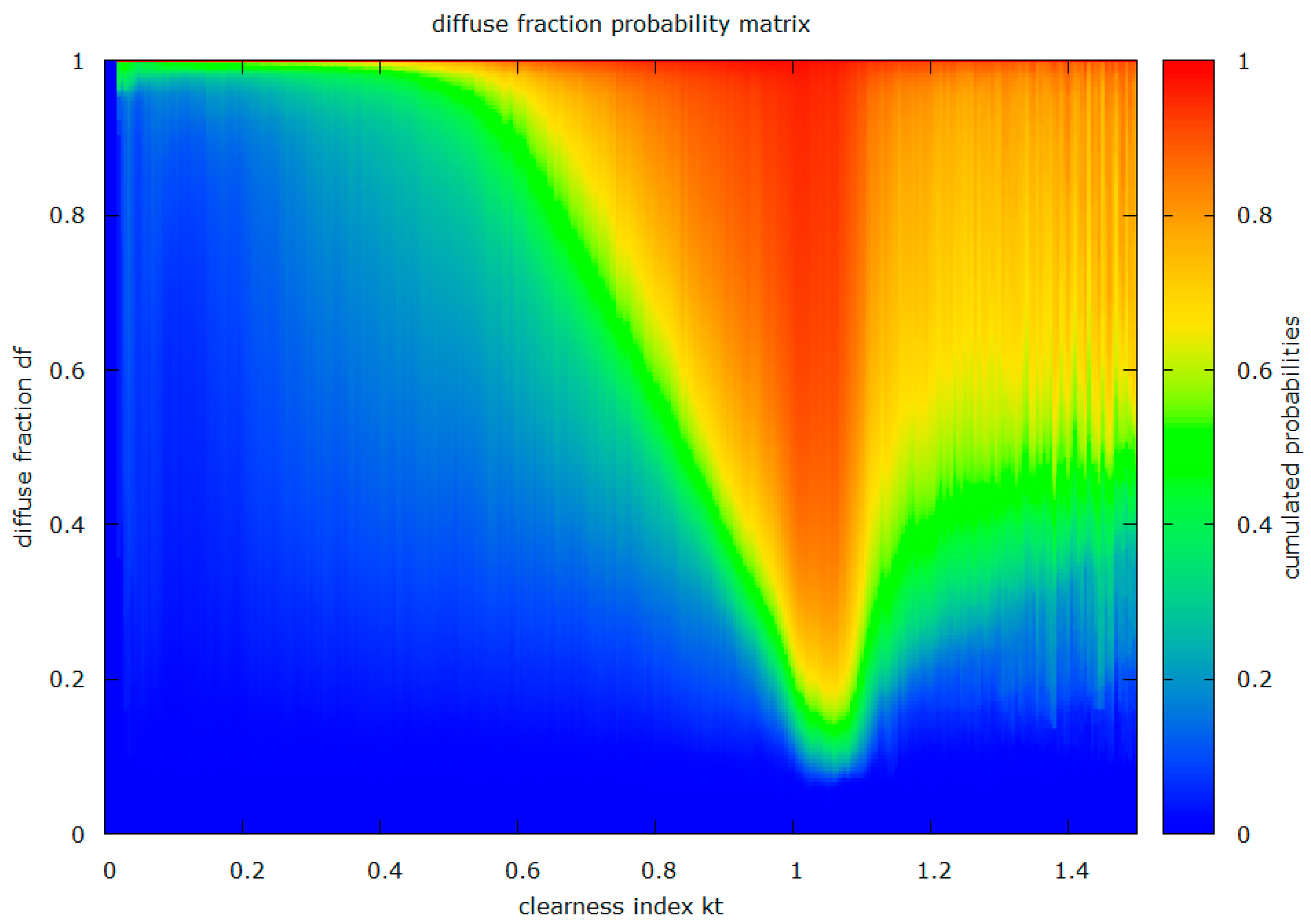
Figure 4 shows an example of such a probability matrix. In the matrix shown here, measurement values from Alice Springs, Australia (2009), Billings, USA (2005), Boulder, USA (2010), Brasilia, Brazil (2011), Cabauw, The Netherlands (2011), Cener, Spain (2010), De Aar, South Africa (2003), Fukuoka, Japan (2013), Gobabeb, Namibia (2013), Lauder, New Zealand (2007), Lerwick, UK (2002), Lindenberg, Germany (2002), Payerne, Switzerland (2010), Regina, Canada (2011), Tateno, Japan (2003) and Xianghe, China (2006) were incorporated.
In order to determine a value for d f for a given k t , the procedure is as follows. Since this is the first part of the new model, the diffuse fraction of this part is referred to as d f 1 :
(1)
Select column of probability matrix that corresponds to the k t value;
(2)
Generate a Markov number r M (randomized number between 0 and 1) [28];
(3)
Select the row where r M is smaller than the cumulated probabilities for the first time;
(4)
The selected row corresponds to d f 1 value.
The usage of real measurement values, incorporated into a matrix of probabilities, holds the advantage of preserving the natural relationship of the diffuse fraction and the clearness index and additionally resulting in a more realistic variability of the modelled d f value series.

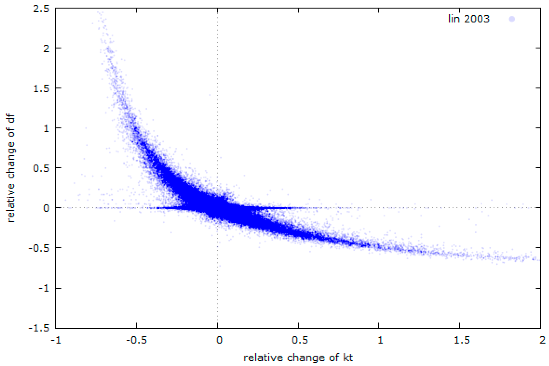
3.2. Part Two. Change of df as Function of Change of kt

By analyzing the extensive BSRN measurement database, a strong correlation has been found between the relative changes of the clearness index (from one minute to the next) to changes of the diffuse fraction. In Figure 5 this correlation is shown for Lindenberg, Germany, for the year 2003.
It was observed that for positive relative changes of k t (when the current k t is higher than the k t one minute before), the diffuse fraction will most likely show a negative relative change. If the relative change of k t is negative, the change of the diffuse fraction will be positive.
There are situations, however, where k t is changing from one minute to the next without an observable change of d f (compare the horizontal value accumulation at d d f = 0 ). These situations are typical for days with rapid irradiance enhancements due to moving broken clouds.
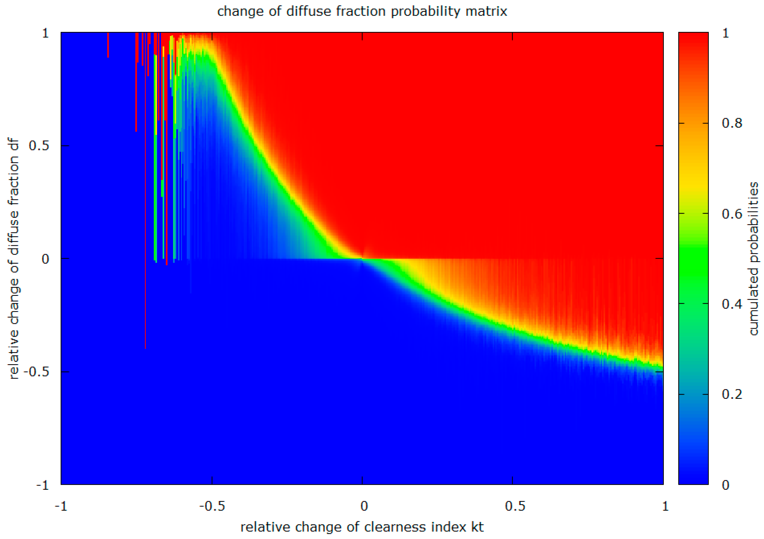
In correspondence to part 1, the relationship between the relative change of d f and the relative change of kt ( d k t ) is also expressed in a matrix of probabilities, displayed in Figure 6. This matrix is only used in the d k t range of −0.5 to 1, since the amount of measurement values outside of this range is too small, which results in unwanted noise. The procedure to retrieve a value for the diffuse fraction in this part, d f 2 , is as follows:
(1)
Calculate the relative change of k t as:
d k t = k t now   /   k t before     1
(2)
For d k t greater than −0.5 and smaller than 1
  • Select the column of the probability matrix that corresponds to d k t ;
  • Generate a Markov number r M (randomized number between 0 and 1) [28];
  • Select the row where r M is smaller than the cumulated probabilities for the first time;
  • The selected row corresponds to change of d f , that is:
    d d f = d f now   /   d f before     1
(3)
For d k t smaller than −0.5, d d f is not taken from the matrix, but extrapolated as:
d d f = 0.5 d k t 4 1.23 d k t 3 + 1.1 d k t 2 0.87 d k t
(4)
For d k t greater than 1, d d f is extrapolated as:
d d f = 0.35 0.15 d k t
(5)
The diffuse fraction for part 2, d f 2 , can now be calculated as:
d f 2 = d d f d f before

3.3. Part Three. Geometric Calculation for Days with Clear Sky

3.3.1. Calculation of the Daily Course of d f

In the case of clear sky, d f is mainly dependent on the air mass relative to its daily minimum. For that reason, in this part of the model a geometric approach has been chosen capable of reproducing the characteristic daily course of the diffuse fraction for clear sky days. The diffuse fraction of this part is calculated as:
d f 3 = A M A M min d f min
The air mass can be modelled as a function of the elevation of the sun. The minimal air mass A M min is calculated for each day by using the maximum elevation angle γ S ,   max :
A M ( min ) = 1 sin ( γ S , ( max ) ) 1.15
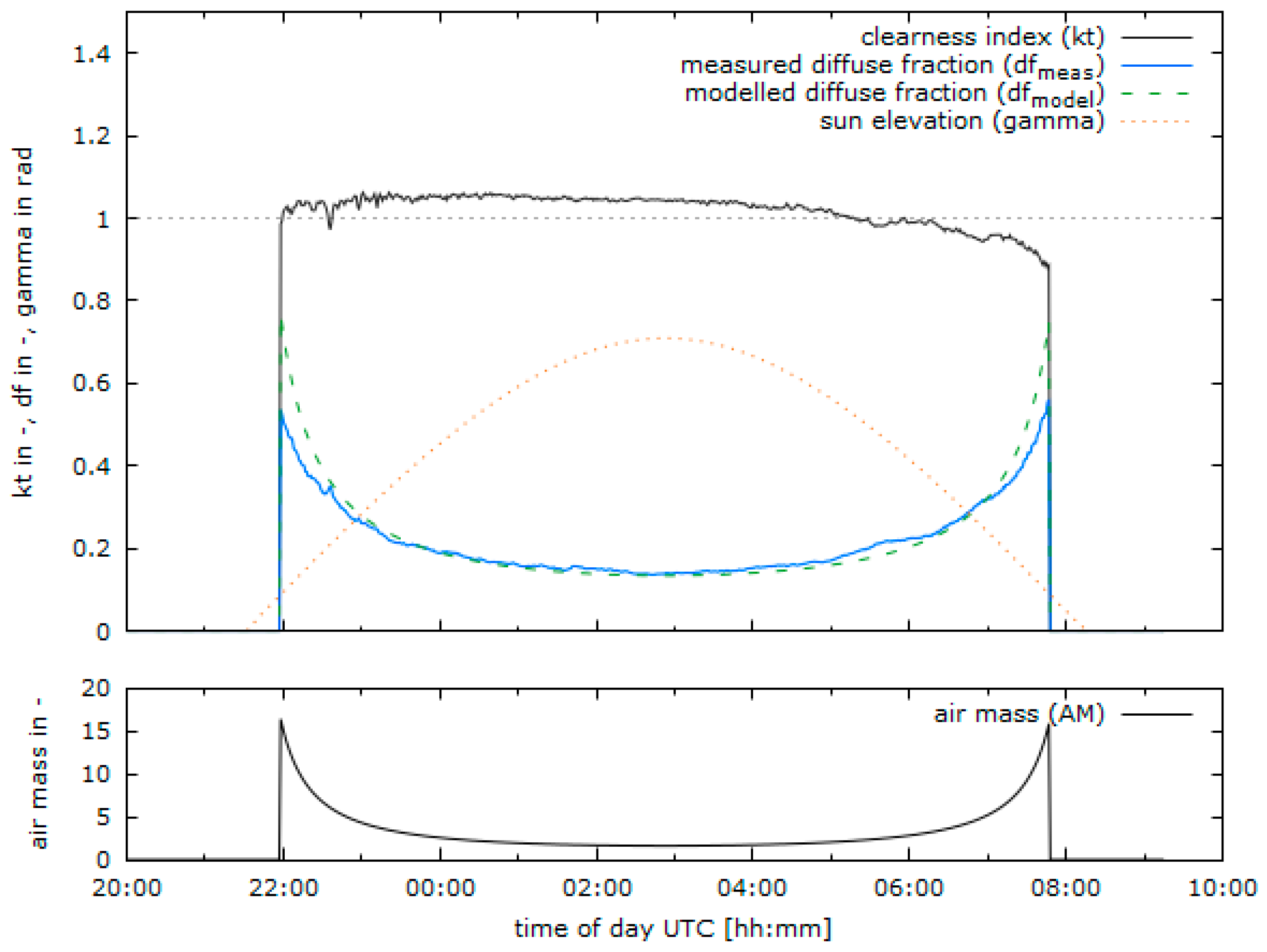
Figure 7 displays the measured (blue) and modelled (green dashed) course of the diffuse fraction over an exemplary day in Tateno, Japan (13 February 2006). While the clearness index k t (black) is relatively stable around 1, the diffuse fraction is around 0.5 shortly after sunrise and before sunset and is falling down to a minimal diffuse fraction d f min at noon, to 0.136 in this example.
However, the main challenge in modelling the diffuse fraction over the course of a clear sky day is to find a good approximation for the minimal diffuse fraction of the day, since this factor is subject to strong variations in every possible respect: from location to location, from season to season and even from day to day.

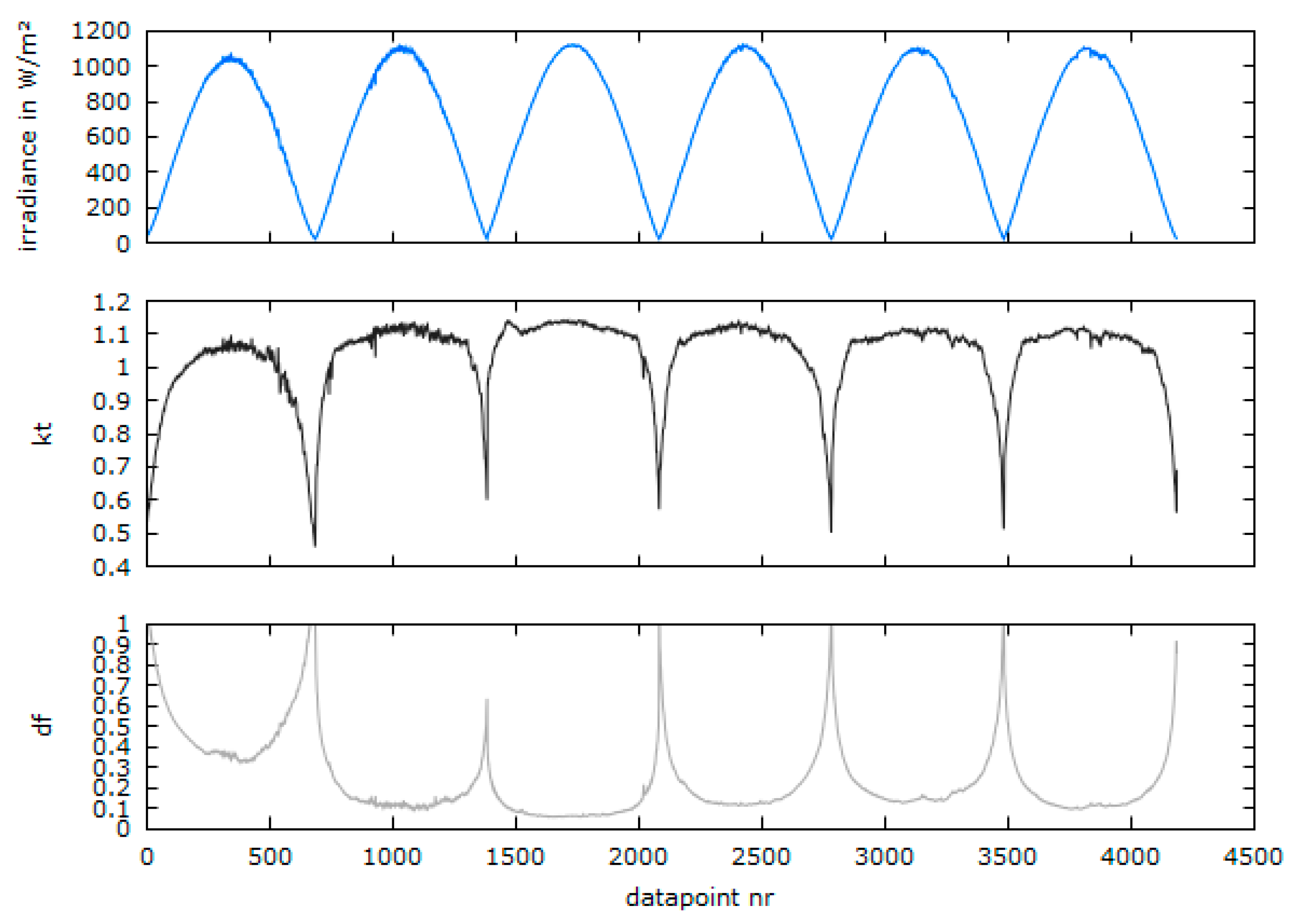
3.3.2. Daily Variation of d f min

In order to illustrate the daily variation of d f min , seven consecutive days in Tamanrasset, Algeria, are shown in Figure 8. Even for this non-cloudy site d f min may vary significantly from day to day: The minimal value of the diffuse fraction (grey, bottom plot) of each day is varying between 0.328 on the first day (21 March 2006) and 0.062 on the third day (23 March 2006).

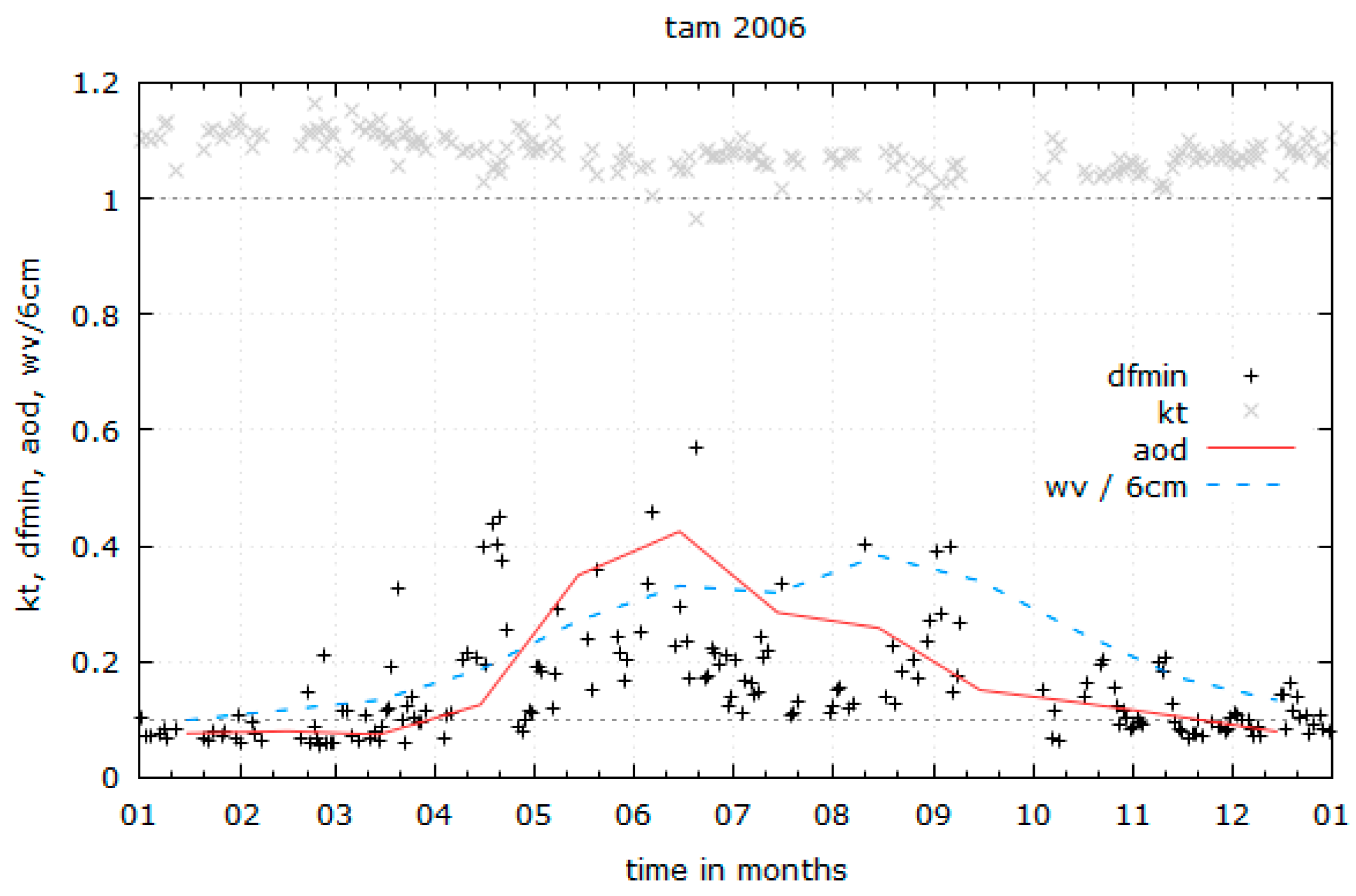
3.3.3. Seasonal Variation of d f min

In addition to daily variations, d f min also shows seasonal variation on some locations. 
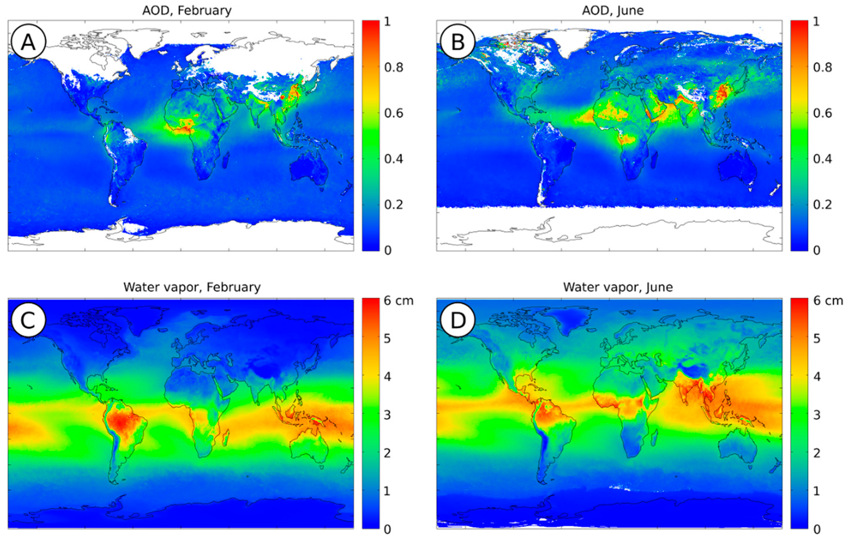
Figure 9 displays the minimal diffuse fractions of all clear days in Tamanrasset, Algeria, in 2006 (black plus symbols) over the course of a year. While in wintertime d f min ranges mostly between 0.05 and 0.15, it almost never falls below 0.1 in summertime and features values between 0.15 and 0.5. When looking at the daily mean k t values (grey crosses), no significant correlation can be observed which implies that other factors must have influence on the minimal daily diffuse fraction. The monthly means of aerosol optical depth (red) and the water vapor (blue dashed) taken from the NASA Terra/MODIS satellite [29,30] however feature a seasonal behavior similar to d f min .

3.3.4. Summary of Factors Influencing d f min

This leads to the conclusion that d f min is dependent on a series of factors. A list of factors that proved influential on d f min is given below:
(1)
The clearness index k t . The values of k t are averaged in a range of 120 min around noon:
k t ¯ = 1 t range i = t noon t range 2 t noon + t range 2 k t i
(2)
The variability of the clearness index, k t Var . For the same period of time, the changes of k t are registered:
k t Var = i = t noon t range 2 t noon + t range 2 | k t i k t i 1 1 |
(3)
The maximum elevation of the sun during the day, γ S , max and the minimum air mass during the day, A M min , compare to top of this section.
(4)
The aerosol optical depth (AOD) and the water vapour (wv) of the respective month. These values are taken from the NASA Terra/MODIS satellite [29,30] and averaged on a month per month basis between 2001 and 2015. Figure 10 gives an impression of the worldwide seasonal characteristics of AOD and wv.
(5)
The up and down time of k t in the morning and in the evening. As a measure of the steepness of the k t curve, the time span is determined between sunrise and when k t first reaches the threshold of 1 in the morning. A second time span between the moment when k t is at last above 1 in the evening and sunset is measured as well. The two values are averaged and are a good indicator for d f min   in places with high day-to-day variation of d f min : The longer the up/down time, the higher d f min will be.

3.3.5. Resulting Equations for d f min

The factors that influence d f min mentioned in the above section are combined in a series of posynomials, depending on the location and availability of data. The coefficients and exponents of the following posynomials were fitted with the help of the Levenberg-Marquardt algorithm implementation of the software gnuplot 5.0 [31].
The datasets used for the posynomial fits are taken from the same locations as in Table 2, but for different years of measurement: asp 2009, bil 2005, bou 2010, brb 2011, cab 2011, cam 2002, clh 2014, cnr 2010, coc 2007, daa 2003, dar 2010, fua 2013, gob 2013, iza 2010, lau 2007, ler 2002, lin 2002, pal 2010, pay 2010, reg 2011, sap 2013, sbo 2011, sms 2006, sov 2002, tam 2003, tat 2003, tor 2005, xia 2006. For Case 1 only the subset bou 2010, iza 2010, sbo 2011, sov 2002, tam 2003 and xia 2006 was used.
Case 1: AOD and water vapor data available, location features strong seasonal changes of AOD (indicator for seasonal aerosol concentrations e.g., due to sandstorms in desert regions, see Table 3 the values for factors a, b and c).
d f min = a 0 k t b 0 + a 1 k t var b 1 + a 2 A M b 2 + a 3 A O D b 4 + a 4 w v b 4 + a 5 t up / down b 5 + c
Case 2: AOD and water vapor data available, no strong seasonal changes of AOD (see Table 4 the values for factors a, b and c).
d f min = a 0 k t b 0 + a 1 k t var b 1 + a 2 A M b 2 + a 3 A O D b 4 + a 4 w v b 4 + a 5 t up / down b 5 + c
Case 3: AOD and water vapor data are not available (see Table 5 the values for factors a, b and c):
d f min = a 0 k t b 0 + a 1 k t var b 1 + a 2 A M b 2 + a 5 t up / down b 5 + c
Case 4: AOD, water vapor and up/down time data are not available (see Table 6 the values for factors a, b and c).
d f min = a 0 k t b 0 + a 1 k t var b 1 + a 2 A M b 2 + c

3.4. Combination of the Three Parts

The three parts of the algorithm generate the values d f 1 , d f 2 and d f 3 . Depending on the current weather situation, expressed by characteristics and statistical features of k t , they are combined to one single, resulting d f :
d f = w 1 d f 1 + w 2 d f 2 + w 3 d f 3
The mean absolute deviation of k t at a given time of day t x that is used as condition above is calculated as follows:
m a d k t = 1 t range i = t x t range t x | k t i k t i 1 1 |
with t range = 30   min 
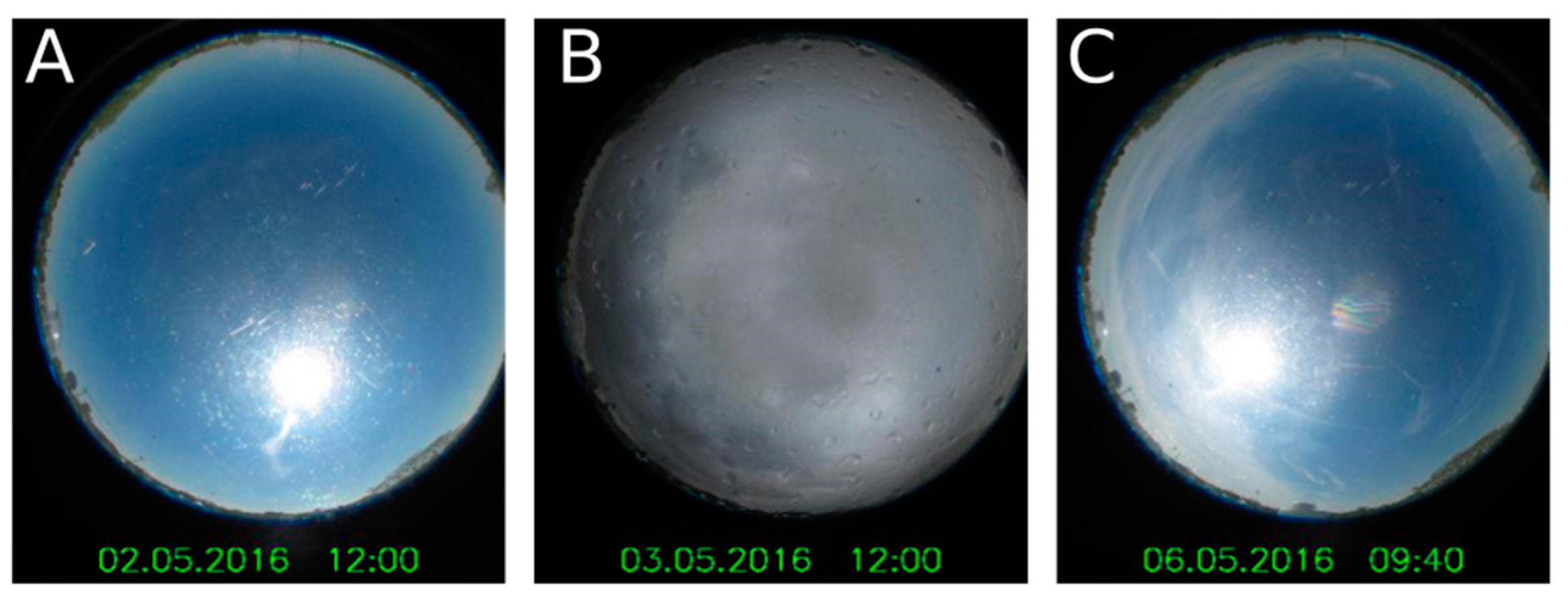
. For illustration of the weighing conditions mentioned in Table 7, Figure 11 displays all-sky camera images from the Institute of Meteorology and Climatology of the Leibniz University Hannover [32,33]. Picture A shows a moment where no clouds are visible. It is classified as “Clear Sky” since k t = 1.03 and m a d k t = 0.0025 . Picture B shows a moment where k t = 0.147 and m a d k t = 0.107 , hence being classified as “Standard”. In picture C some light clouds are visible around the sun. This moment is classified as “Transition” as k t = 1.01 and m a d k t = 0.028 . The “Transition” condition can be interpreted as clear sky with only few light clouds.
The generated matrices and other model data can be obtained from the authors upon request.

4. Results

In this section, the results of the validation of the new algorithm are presented. As mentioned in Section 2.1, the validation is conducted for 28 locations with one year of one-minute values each, basing the validation on more than seven million data points worldwide.
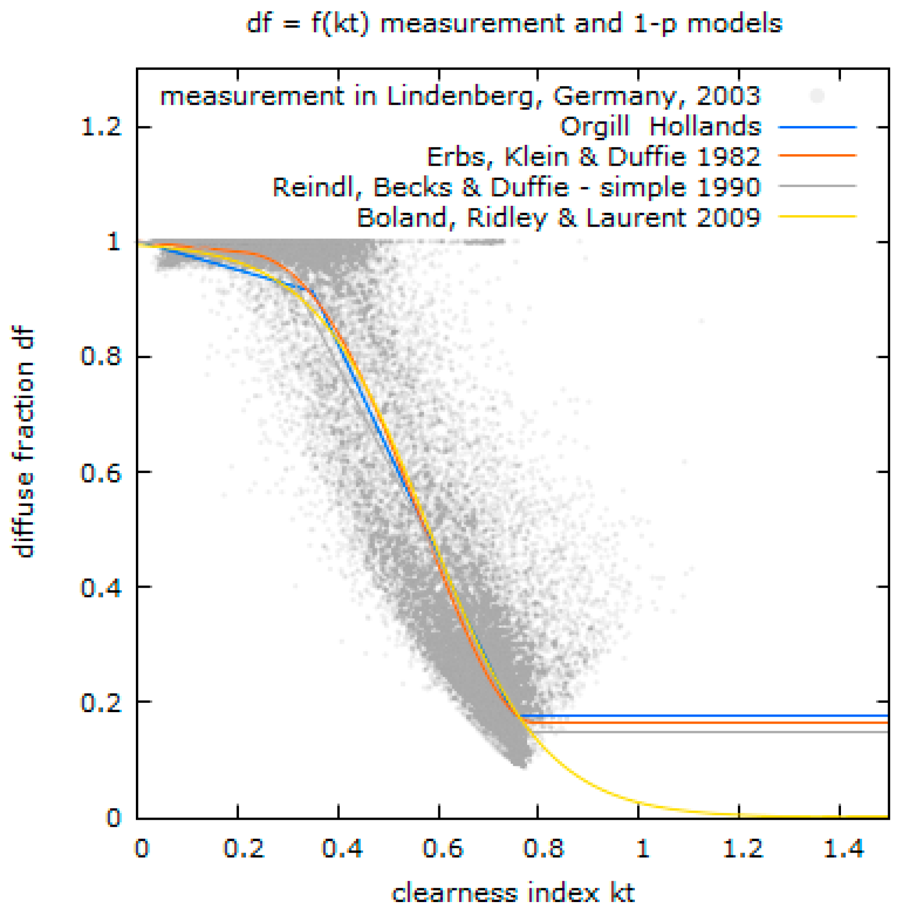
The overall results are then compared to the results of three existing models for the diffuse fraction: the model of Orgill and Hollands [18] (OH), a one-parameter model, the reduced version of the two-parameter model of Reindl et al. [3] (RR), and the model by Perez and Ineichen [23] (PZ), all introduced in Section 2.3. The first two models were also identified as two of the three best performing models among the eight investigated approaches by Dervishi [27]. The model by Perez and Ineichen [23] is still popular in the community and widely made use of. The model by Skartveit [12] was not used for the model comparison since no indications were found that show a significant advantage of this model over Orgill and Hollands [18], Reindl et al. [3] or Perez and Ineichen [23].
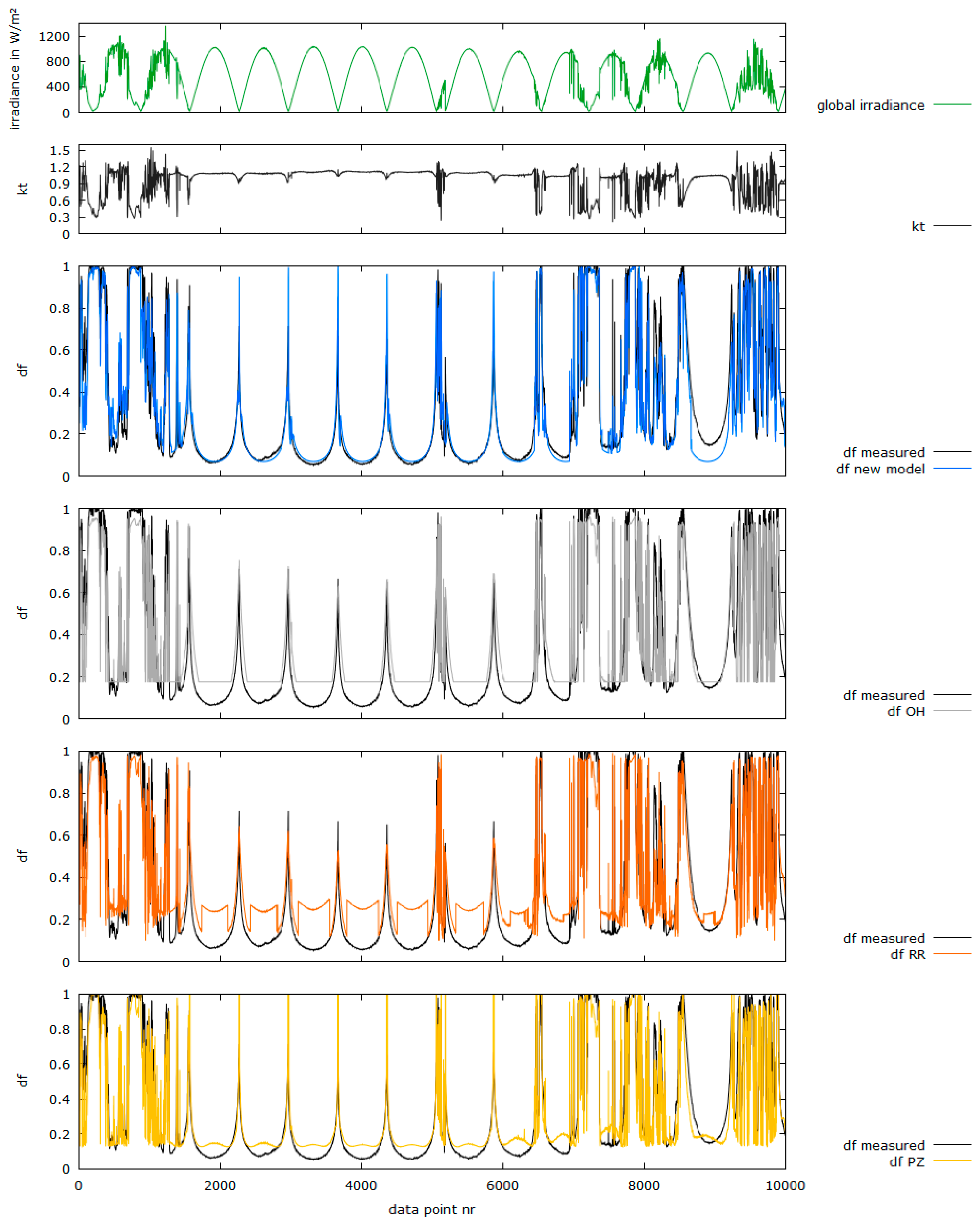
Figure 12 displays two weeks in Alice Springs, Australia, 2005. The measured global horizontal irradiance is plotted on top (green); the resulting clearness index k t is plotted for reference underneath (black). In the three following plots, the measured diffuse fraction (black) is displayed, together with the diffuse fraction that was modelled with the new approach (blue), with the model from Orgill and Hollands [18] (grey) , the model from Reindl et al. [3] (orange) and the model from Perez and Ineichen [23].
While the new model is able to reproduce the diffuse fraction in good accordance to the measurement values most of time, the inherent problem of models with static one- or two-parameter relationships between the clearness index and the diffuse fraction becomes apparent. Especially on clear sky days the existing models fail to reproduce the characteristic behavior of the diffuse fraction.
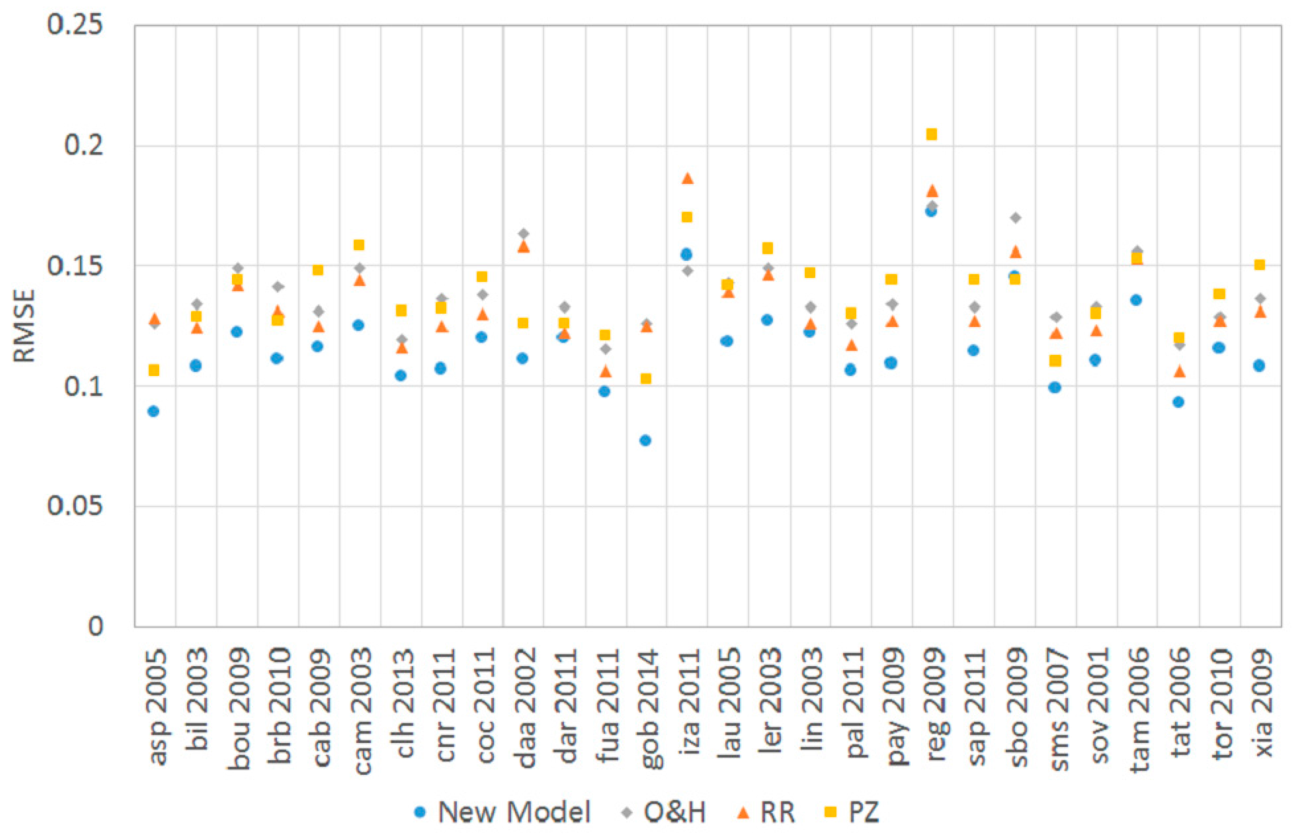
In order to evaluate the performance of the new model in statistical terms, the root mean squared errors (RMSEs) are calculated for the new model as well as for the three reference models. Figure 13 shows the RMSE for the four models over all test data sets. The RMSE produced by the new model is smaller than those produced by the models of Orgill and Hollands [18], Reindl et al. [3] and Perez and Ineichen [23], in parts significantly, except for one case in Izaña, Spain, 2011 (iza 2011). The overall RMSE, averaged over all test data sets, can be reduced from 0.138 (OH), 0.134 (RR) and 0.139 (PZ) to 0.116 for the new model, which equals an amelioration of 16%–20%.
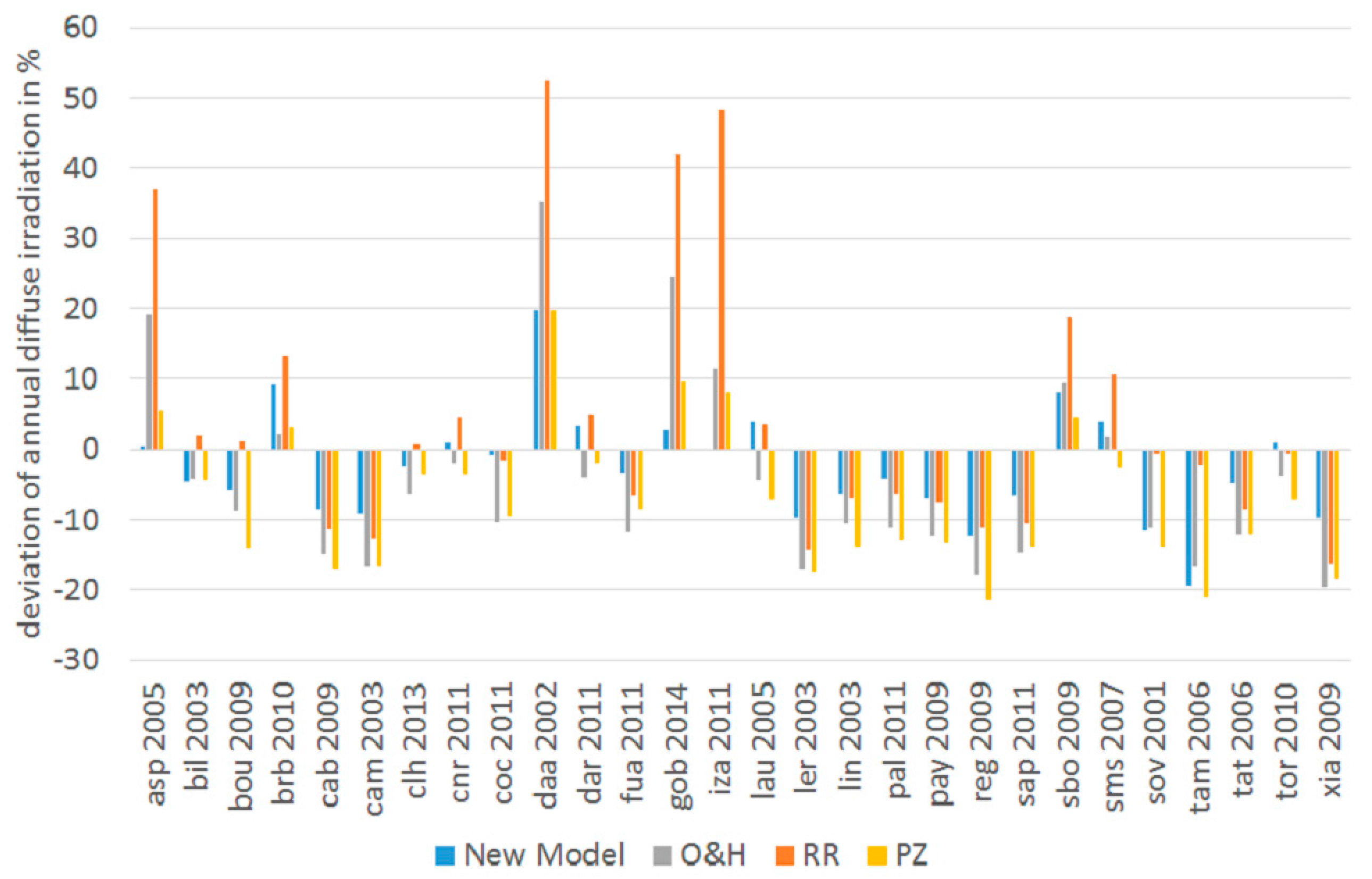
A further validation is conducted by comparing the annual diffuse irradiation values that are estimated by the models with the measured value. Figure 14 lists the relative deviations of the modelled from the measured annual diffuse irradiation. In most of the cases, the deviation resulting from the new model is significantly smaller than the deviation resulting from the models of OH, RR or PZ. There are few cases where the model leads to higher deviations than the existing ones, e.g., for Billings, USA (bil 2003), Solar Village, Saudi Arabia (sov 2001) or Tamanrasset, Algeria (tam 2006). Extreme deviations of more than 20%, however, as apparent in some of the test cases for the two existing models, do not occur when using the new model. The average of the absolute (i.e. unsigned) relative deviations for all test cases can be reduced by nearly 50% from 11.9% for OH, 12.7% for RR and 10.9% for PZ to only 6.4% for the new model.
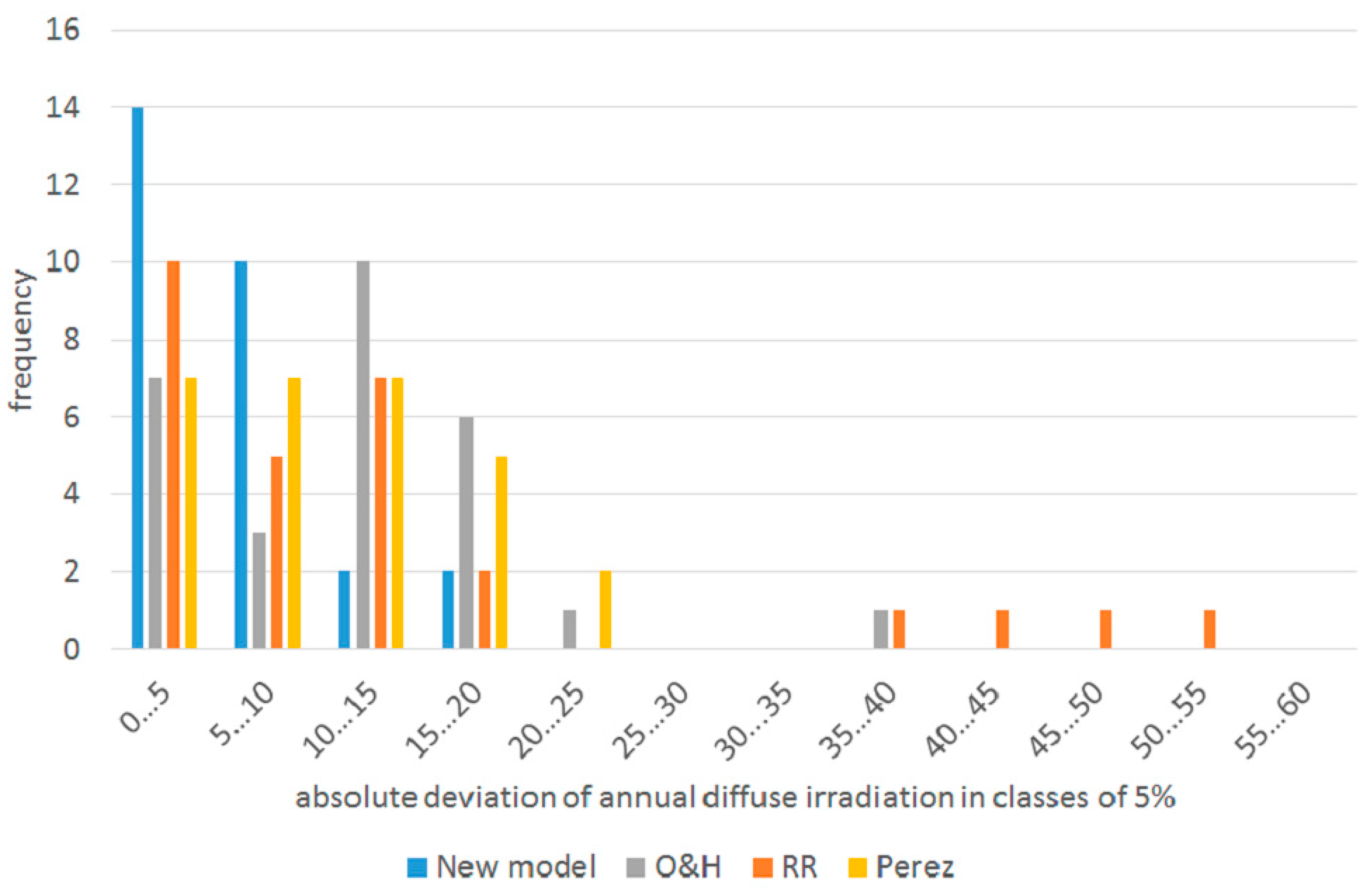
The histogram of the mean absolute deviations of the annual diffuse irradiation displayed in Figure 15 illustrates the frequency of the deviations each model produces. While the model of Reindl et al. [3] (RR) has its peak in the class of 0 to 5%, it still has several outliers of 35%–55%. The model of Orgill and Hollands [18] (OH) features only one extreme outlier at 35%–40%, but has most of its results lying in the class of 10 to 15%. The model by Perez and Ineichen [23] shows no outliers of more than 25% but has its results evenly distributed between 0 and 15%. The new model does not produce any outliers and has its peak in the class of 0%–5%, covering 50% of the test cases alone.
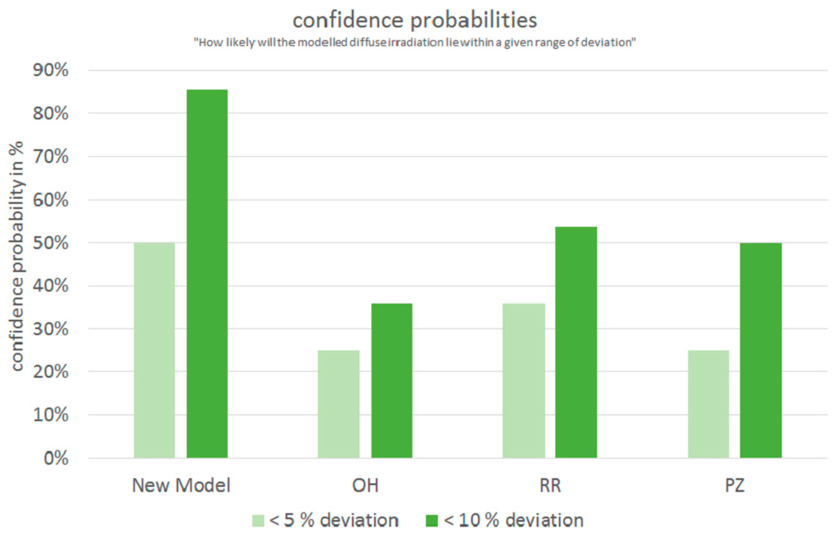
This histogram can be converted into confidence probabilities, depicted in Figure 16. The new model results in mean absolute deviations of less than 5% in 50% of the cases. In more than 80% of the cases, the deviation is less than 10%. Compared to the other three models this is a significant improvement, where the probability of producing less than 5% deviation is only 25% (OH), 36% (RR) and 25% (PZ) and the probability of producing less than 10% deviation is 36% (OH), 54% (RR) and 50% (PZ).

5. Conclusions

The newly developed model for the diffuse fraction of solar irradiance on PV systems provides significantly better agreement with measurements than the other models published so far. This is achieved by the following features: the first part utilizes the dependency of the diffuse fraction d f on the clearness index k t , in analogy to existing one-parameter models. In the new model, the correlation is expressed as probability matrices rather than single functions, leading to realistic, more natural diffuse fraction characteristics. Also taking advantage of probability matrices, the second part uses the relation of the relative changes of d f over the relative changes of k t . The third part takes into account the diffuse fraction characteristics of days with clear sky only using a geometrical approach. The crucial factor for the third part is the minimum daily diffuse fraction for which a posynomial model has been introduced.
The presented new model was analyzed and compared to two other models for 28 locations worldwide with one year of one-minute measurement data each. It was shown that the new model has a high quality of modeling the diffuse irradiance. The mean RMSE over all test cases was reduced by 16%–20%, whereas the mean absolute deviation of the annual diffuse irradiation was found to be nearly 50% smaller compared to the reference models. In more than 80% of the test cases, the deviation of the annual diffuse irradiation is smaller than 10%, with an overall maximum deviation of 20%.
With the new model, the diffuse irradiance can be calculated with much lower uncertainty, hence significantly reducing the uncertainty of PV energy yield simulations. Possible future work for the improvement of the model will include further investigations on the minimal daily diffuse fraction that has a very decisive influence on the model quality for clear sky days. Such days may be identified by cloud cameras that will allow for a much better estimation of the cloud fraction compared to satellite images [33].

Acknowledgments

The publication of this article was funded by the Open Access Fund of the Leibniz Universität Hannover.

Author Contributions

The research and development of the algorithm, as well as the algorithm comparisons and the writing of the paper was conducted by Martin Hofmann. Gunther Seckmeyer gave valuable input to former work on the topic (see Section 2.3), discussed the results and revised the manuscript critically.

Conflicts of Interest

The authors declare no conflict of interest.

References

  1. Spencer, J.W. A comparison of methods for estimating hourly diffuse solar radiation from global solar radiation. Solar Energy 1982, 29, 19–32. [Google Scholar] [CrossRef]
  2. König-Langlo, G.; Sieger, R. Report of the 12th Baseline Surface Radiation Network (BSRN) Scientific Review and Workshop; WCRP Report No. 20/2012; Alfred Wegener Institute (AWI): Potsdam, Germany, 1–3 August 2012. [Google Scholar]
  3. Reindl, D.T.; Beckman, W.A.; Duffie, J.A. Diffuse fraction correlations. Solar Energy 1990, 45, 1–7. [Google Scholar] [CrossRef]
  4. Hay, J.E.; Davies, J.A. Calculations of the solar radiation incident on an inclined surface. In Proceedings—First Canadian Solar Radiation Data Workshop; Hay, J.E., Won, T.K., Eds.; Ministry of Supply and Services Canada: Ottawa, ON, Canada, 1980; p. 59. [Google Scholar]
  5. PV*SOL 2017 R5. Valentin Software GmbH, Berlin, Germany. 2016. Software. Available online: http://www.valentin-software.com (accessed on 21 December 2016).
  6. Feldman, D.; Bolinger, M. On the Path to SunShot: Emerging Opportunities and Challenges in Financing Solar; NREL/TP-6A20-65638; National Renewable Energy Laboratory: Golden, CO, USA, 2016.
  7. Köppen, W. Klassifikation der Klimate nach Temperatur, Niederschlag und Jahreslauf. Petermanns Geogr. Mitt. 1918, 64, 193–203, 243–248. [Google Scholar]
  8. Reda, I.; Andreas, A. Solar position algorithm for solar radiation applications. Solar Energy 2004, 76, 577–589. [Google Scholar] [CrossRef]
  9. Bourges, G. Reconstitution Des Courbes de Fréquence Cumulées de L'irradiation Solaire Globale Horaire Reçue Par Une Surface Plane; Report CEE 295-77; ESF of Centre d’Energétique de l’Ecole Nationale Supérieure des Mines de Paris, Tome II: Paris, France, 1979. (In French) [Google Scholar]
  10. Maxwell, E.L. A Quasi-Physical Model for Converting Hourly Global Horizontal to Direct Normal Insolation. Available online: http://rredc.nrel.gov/solar/pubs/PDFs/TR-215-3087.pdf (accessed on 21 December 2016).
  11. Hofmann, M.; Riechelmann, S.; Crisosto, C.; Mubarak, R.; Seckmeyer, G. Improved synthesis of global irradiance with one-minute resolution for PV system simulations. Int. J. Photoenergy 2014, 2014, 808509. [Google Scholar] [CrossRef]
  12. Skartveit, A.; Olseth, J. A model for the diffuse fraction of hourly global radiation. Solar Energy 1987, 38, 271–274. [Google Scholar] [CrossRef]
  13. Nack, M.; Green, A. Influence of clouds, haze, and smog on the middle ultraviolet reaching the ground. Appl. Opt. 1974, 13, 2405–2415. [Google Scholar] [CrossRef] [PubMed]
  14. Seckmeyer, G.; Mayer, B.; Bernhard, G.; Erb, R.; Albold, A.; Jäger, H.; Stockwell, W.R. New maximum UV irradiance levels observed in Central Europe. Atmos. Environ. 1997, 31, 2971–2976. [Google Scholar] [CrossRef]
  15. Liu, B.; Jordan, R. The interrelationship and characteristic distribution of direct, diffuse and total solar radiation. Solar Energy 1960, 4, 1–19. [Google Scholar] [CrossRef]
  16. Carroll, J.J. Global transmissivity and diffuse fraction of solar radiation for clear and cloudy skies as measured and as predicted by bulk transmissivity models. Solar Energy 1985, 35, 105–118. [Google Scholar] [CrossRef]
  17. Zernikau, F. Vergleich und Bewertung von Diffusstrahlungsmodellen. Master’s Thesis, Institut für Energietechnik, Technical University of Berlin, Berlin, Germany, 2015. [Google Scholar]
  18. Orgill, J.F.; Hollands, K.G.T. Correlation equation for hourly diffuse radiation on a horizontal surface. Solar Energy 1976, 19, 357–359. [Google Scholar] [CrossRef]
  19. Erbs, J.A.; Klein, S.A.; Duffie, J.A. Estimation of the diffuse radiation fraction for hourly, daily and monthly average global radiation. Solar Energy 1982, 18, 293–302. [Google Scholar] [CrossRef]
  20. Boland, J.; Ridley, B. Modelling of diffuse solar fraction with multiple predictors. Renew. Energy 2010, 35, 478–483. [Google Scholar]
  21. Oliveira, A.; Escobedo, J.; Machado, A.; Soares, J. Correlation models of diffuse solar-radiation applied to the city of São Paulo, Brazil. Appl. Energy 2002, 71, 59–73. [Google Scholar] [CrossRef]
  22. Furlan, C.; Oliveira, A.; Soares, J.; Codato, G.; Escobedo, J. The role of clouds in improving the regression model for hourly values of diffuse solar radiation. Appl. Energy 2012, 92, 240–254. [Google Scholar] [CrossRef]
  23. Perez, R.; Ineichen, P.; Maxwell, E.; Seals, R.; Zelenka, A. Dynamic global-to-direct irradiance conversion models. ASHRAE Trans. Res. Ser. 1992, 98, 354–369. [Google Scholar]
  24. Kambezidis, H.D.; Psiloglou, B.E.; Gueymard, C. Measurements and models for total solar irradiance on inclined surface in Athens, Greece. Solar Energy 1994, 53, 177–185. [Google Scholar] [CrossRef]
  25. Jacovides, C.; Tymvios, F.; Assimakopoulos, V.; Kaltsounides, N. Comparative study of various correlations in estimating hourly diffuse fraction of global solar radiation. Renew. Energy 2006, 31, 2492–2504. [Google Scholar] [CrossRef]
  26. Wong, L.T.; Chow, W.K. Solar radiation model. Appl. Energy 2001, 69, 191–224. [Google Scholar] [CrossRef]
  27. Dervishi, S.; Mahdavi, A. Computing diffuse fraction of global horizontal solar radiation: A model comparison. Solar Energy 2012, 86, 1796–1802. [Google Scholar] [CrossRef] [PubMed]
  28. Markov, A. Extension of the Limit Theorems of Probability Theory to a Sum of Variables Connected in a Chain. Appendix B of: Howard R. Dynamic Probabilistic Systems, 1: Markov Chains; John Wiley and Sons: New York, NY, USA, 1971. [Google Scholar]
  29. MODIS Atmosphere L2 Water Vapor Product. Available online: http://modis-atmos.gsfc.nasa.gov/MOD05_L2/doi.html (accessed on 21 December 2016).
  30. Levy, R.; Hsu, C. MODIS Atmosphere L2 Aerosol Product; NASA MODIS Adaptive Processing System; Goddard Space Flight Center: Greenbelt, MD, USA, 2015.
  31. Williams, T.; Kelley, C. Gnuplot 5, An Interactive Plotting Program. Available online: http://www.gnuplot.info/ (accessed on 21 December 2016).
  32. Tohsing, K.; Schrempf, M.; Riechelmann, S.; Seckmeyer, G. Validation of spectral sky radiance derived from all-sky camera images—A case study. Atmos. Meas. Tech. 2014, 7, 2137–2146. [Google Scholar] [CrossRef] [Green Version]
  33. Werkmeister, A.; Lockhoff, M.; Schrempf, M.; Tohsing, K.; Liley, B.; Seckmeyer, G. Comparing satellite- to ground-based automated and manual cloud coverage observations—A case study. Atmos. Meas. Tech. 2015, 8, 2001–2015. [Google Scholar] [CrossRef] [Green Version]
Figure 1. Top: Measured (grey) and modelled (green) time series of diffuse irradiance on a horizontal surface for four days in Lindenberg, Germany. Global irradiance (blue) for reference. The calculation of diffuse irradiance in this example was done with the reduced model of Reindl et al. [3]. The model underestimates the four-day sum of the diffuse irradiation by 18%. Middle: The global irradiance on a tilted photovoltaic (PV) module (facing south, tilted by 30°) for the same four days. The model used for calculating the irradiance on a tilted surface is from Hay and Davies [4]. Due to the underestimation of the diffuse irradiance (see top), the four-day sum of the global irradiation on the PV module based on modelled values falls below the global irradiation based on measured values by −9%. Bottom: The resulting cumulated deviation of the modelled global irradiation on the tilted plane from the measured. The plot shows that one of the main sources of deviation is the modelling of highly variable irradiance situations, as observed e.g., on 10 June, between 08:00 and 12:00.
Energies 10 00248 g001
Figure 2. Measured diffuse fraction over clearness index k t   for one year of measurement (grey points, extract of 2003) in Lindenberg, Germany. Line plots: Schematic overview of existing one-parameter models. Typically the models define three sections with varying d f = f ( k t ) functions.
Energies 10 00248 g002
Figure 3. Measured diffuse fraction over clearness index k t   for one year of measurement (grey points, extract of 2003) in Lindenberg, Germany. Line plots: The model by Reindl, Beckman and Duffie [3] (reduced version), using two parameters ( k t and sun height) as input.
Energies 10 00248 g003
Figure 4. A probability matrix of the diffuse fraction as a function of the clearness index kt. For each value of k t , this matrix describes the probability with which a certain value of diffuse fraction will occur. The matrix correlates with the existing simple one-parameter models mentioned in Section 2.3, but it is based on measurements. Therefore the natural variability is better described by the model especially for high values of k t ( k t > 1.1, irradiance enhancement due to reflections by broken clouds) while preserving the strong relation at low levels of k t ( k t < 0.4, overcast sky).
Energies 10 00248 g004
Figure 5. Scatter plot of the relative changes of the diffuse fraction over the relative changes of the clearness index for Lindenberg, Germany, 2003. This strong relation is very valuable for modelling a realistic behaviour of the diffuse fraction over the day, since it depends highly on the behaviour of k t . The area where the change of df is 0 while kt shows relatives changes between −0.5 and 0.5, i.e., d f is changing while k t is not, indicates days with movement of broken clouds, the reflection on which couses the measured global irradiance to change rapidly without changing its diffuse fraction.
Energies 10 00248 g005
Figure 6. The same relation between changes of d f and changes of k t as in Figure 5, here as the probability matrix that is used in the model, corresponding to Figure 4. In the model, only relative k t changes of −0.5 to 1 are computed with this matrix. In the matrix shown here, measurement values from the same locations and years as in Figure 4 were incorporated.
Energies 10 00248 g006
Figure 7. Example for the geometric approach used to model clear sky diffuse fraction. The data shown is from Tateno, Japan, for 13 February 2006. While k t (top plot, black) remains relatively constant, the measured diffuse fraction (blue) follows a typical scheme, starting with high d f values in the morning, falling to a minimum at noon and rising again in the evening. This behaviour shows a strong correlation with the change of the air mass during the day (bottom plot, black). The clear sky diffuse fraction (green) is modelled as presented in Equation (9). The most important factor in this part of the model is the smallest value of d f during the day, d f min . Modelling d f min correctly is crucial for good algorithm results.
Energies 10 00248 g007
Figure 8. Measurement values for global irradiance (blue, top), k t (black, center) and d f (grey, bottom) for Tamanrasset, Algeria, from 21 to 26 March 2006. This plot illustrates the variation of the minimum daily d f value ( d f min ) for consecutive clear sky days. d f min values for March 21 to 26 are: 0.328, 0.101, 0.062, 0.123, 0.139 and 0.105. One factor of influence seems to be the averaged maximum value of k t around noon. Another indicator is the shape of the k t curve during day: A slow rise of k t in the morning and slow fall in the evening indicate a high d f min like on 21 March, whereas steep ramps in the morning and evening with flat trends during the day indicate low d f min value (e.g., 26 March).
Energies 10 00248 g008
Figure 9. Variation of d f min (black) of days with clear skies over a year in Tamanrasset, 2006. While d f min is mostly close to 0.1 in wintertime, it varies strongly from spring to autumn, with no clear relation to the mean clearness index of the corresponding day (grey). It was found that changing levels of aerosols (red) and water vapour (dotted blue) may cause this effect.
Energies 10 00248 g009
Figure 10. Monthly means of aerosol optical depth (AOD) (plots A and B) and water vapour (C,D) for February (A,C) and June (B,D), from 2001 to 2015. Data taken from NASA Terra/MODIS satellite [29,30].
Energies 10 00248 g010
Figure 11. Three pictures made by an Hemispherical Sky Imager in Hannover (at the Institute for Meteorology and Climatology of the Leibniz University Hannover) in order to illustrate the three different weighing conditions presented in Table 7. Time in UTC. (A) 02 May 2016 12:00–Clear Sky: k t = 1.03 , m a d k t = 0.0025 ; (B) 03 May 2016 12:00–Standard: k t = 0.147 , m a d k t = 0.107 ; (C) 06 May 2016 09:40–Transition: k t = 1.01 , m a d k t = 0.028 .
Energies 10 00248 g011
Figure 12. Plot of measured and modelled irradiance values for 14 consecutive days in Alice Springs, Australia, 2005, as an example. The total amount of analysed data sets comprises one year in minutes for each of the 28 test cases (refer to Section 2.1), equaling to seven million datapoints. Values at night are omitted in this plot. The measured global irradiance (green) is shown on top, the resulting clearness index k t (black) for reference in the middle. The bottom part of the diagram displays measured (black) and modelled diffuse fractions (blue for the new model, grey for Orgill and Hollands [18], orange for Reindl et al. [3], yellow for Perez and Ineichen [23]). Most of the time, the output of the new model leads to good conformity for clear sky days as well as for days with broken clouds. The inherent problem of static one- or two-parameter models becomes apparent when comparing the measurement values to the output of the models by Orgill and Hollands [18], Reindl et al. [3] and Perez and Ineichen [23], especially for clear sky days.
Energies 10 00248 g012
Figure 13. The root mean squared errors (RMSE) for all analysed datasets of the modelled versus the measured diffuse fraction. The RMSE of the new model is in all cases smaller than the RMSE of the model by Orgill and Hollands [18] (OH, grey), Reindl et al. [3] (RR, orange) or Perez and Ineichen [23] (PZ, yellow), except for the location of Izaña, Spain (iza 2011), where the OH model produces a slightly smaller RMSE. The mean RMSE over all test cases is at 0.116 for the new model, 0.138 for OH, 0.134 for RR and 0.139 for PZ, which implies an amelioration of the RMSE of 16%–20%.
Energies 10 00248 g013
Figure 14. Relative deviation of the modelled annual diffuse irradiation from the measured diffuse irradiation for all analysed datasets. The new model performs better than the three reference models by Orgill and Hollands [18] (OH, grey), Reindl et al. [3] (RR, orange) and Perez and Ineichen [23] in nearly all cases, except for desert-like locations such as Solar Village, Saudi Arabia (sov) or Tamanrasset, Algeria (tam). None of the test cases shows deviations of more than ±20% for the new model. The mean absolute deviation over all test cases for the new model is 6.4%, whereas it reaches 11.9% for OH, 12.7% for RR and 10.9% for PZ. The mean absolute deviation can thus approximately be halved when using the new model.
Energies 10 00248 g014
Figure 15. Histogram of the mean absolute deviations of the annual diffuse irradiation in classes of 5%. Most of the deviations produced by the new model are smaller than 10% (compare Figure 16). In none of the test cases deviations of more than 20% can be observed. While the model by Reindl et al. [3] (RR, orange) has most of its test cases in classes <15%, it still produces in some cases results of more than 40%. The model of Orgill and Hollands [18] (OH, grey) features less extreme deviations but shows a strong frequency of deviations between 10% and 20%. The model by Perez and Ineichen [23] (PZ, yellow) does not produce outliers and has its results distributed evenly between 0 and 15%.
Energies 10 00248 g015
Figure 16. When using the new model for calculating the diffuse irradiance, the annual deviation of the modelled irradiation will be smaller than 5% in more than 40% of the cases, and smaller than 10% in over 80% of the cases. When using the model of Orgill and Hollands [18] (OH), these confidence probabilities reduce to 25% and 36%, while using the model of Reindl et al. [3] (RR) reduces the probabilities to 36% and 54% respectively. The use of the model of Perez and Ineichen [23] (PZ) results in probabilities of 25% and 50%.
Energies 10 00248 g016
Table 1. Measured and modelled diffuse irradiation for Lindenberg, Germany (LIN), and Gobabeb, Namibia (GOB). The top section refers to the figures above, time ranges from 10–13 May 2003. The modelled underestimation of the diffuse irradiation by −17.9% leads to an underestimation of the global irradiation on the tilted PV module by −9.3%, hence leading to an underestimation of the simulated PV energy yield by 8.3%. When considering the whole year (2nd section), the modelled diffuse irradiation differs from the measured value by −7.2%, leading to an underestimation of the irradiation on module surface by −3.1%. The difference in the annual PV energy yield is −2.7%. In the 3rd and 4th section, the results of the same analysis are presented for Gobabeb, Namibia. Here, the PV module faces North and is tilted at 23°. The modelled sum of diffuse irradiation for selected days (23–26 July 2014) is 20.4% higher than the measured sum, leading to a deviation in the PV energy of 4.4%. Over the whole year of 2014, the deviation of the diffuse irradiation is even 42%, which causes a difference in the annual PV yield of 7.6%.
LIN, 10–13 May 2003Unitwith Measured DataModelledDeviation
Global horizontal irradiationkWh/m²19.7--
Diffuse irradiationkWh/m²12.09.9–17.9%
Global irradiation on tilted surfacekWh/m²22.620.5–9.3%
PV energy yieldkWh65.660.2–8.3%
LIN, whole year 2003Unitwith Measured DataModelledDeviation
Global horizontal irradiationkWh/m²1185.1--
Diffuse irradiationkWh/m²555.9515.7–7.2%
Global irradiation on tilted surfacekWh/m²1467.01422.0–3.1%
PV energy yieldkWh4339.24221.4–2.7%
GOB, 23–26 July 2014Unitwith Measured DataModelledDeviation
Global horizontal irradiationkWh/m²18.2--
Diffuse irradiationkWh/m²4.65.520.4%
Global irradiation on tilted surfacekWh/m²22.523.75.0%
PV energy yieldkWh66.269.14.4%
GOB, whole year 2014Unitwith Measured DataModelledDeviation
Global horizontal irradiationkWh/m²2433.1--
Diffuse irradiationkWh/m²454.9645.842.0%
Global irradiation on tilted surfacekWh/m²2401.92600.88.3%
PV energy yieldkWh6808.77325.47.6%
Table 2. Overview over the 28 datasets that were used in this work. The locations are spread over the globe between −45° South and 52° North. Height above sea level, surface, topography and climate zones (according to Köppen [7]) show a high level of variation. The years of measurement were chosen to provide a high annual completeness of measurement (ACM), i.e., as few missing data points as possible. The total resulting amount of data points that is used in the following analysis exceeds 14.7 million (or approximately 7 million when omitting night time).
IDNameCountryLatitude in °Longitude in °Height in mTime ZoneSurfaceTopographyClimate ZoneACM in %
ASP 2005Alice SpringsAustralia–23.798133.8885479.5grassflat, ruralBWh99.4
BIL 2003BillingsUSA36.605–97.516317–6grassflat, ruralCfa99.6
BOU 2009BoulderUSA40.05–105.0071577–7grassflat, ruralBSk99.0
BRB 2010BrasiliaBrasil–15.601–47.7131023–3concreteflat, ruralAw96.6
CAB 2009CabauwNetherlands51.9714.92701grassflat, ruralCfb99.1
CAM 2003CamborneUK50.217–5.317880grassflat, ruralCfb90.4
CLH 2013Chesapeake LightUSA36.905–75.71337–5water, oceanflat, ruralCfa99.8
CNR 2011CenerSpain42.816–1.6014711asphaltmountain valley, urbanCfb99.8
COC 2011Cocos IslandsCocos Islands–12.19396.835–16.5n.a.n.a.Af95.6
DAA 2003De AarSouth Africa–30.66723.99312872sandflat, ruralBSk88.1
DAR 2011DarwinAustralia–12.425130.891309.5grassflat, ruralAw100
FUA 2011FukuokaJapan33.582130.37539asphaltflat, urbanCfa99.9
GOB 2014GobabebNamibia–23.56115.0424071n.a.flat ruralBWh100
IZA 2011IzañaSpain28.309–16.4992372.90rockmountain topCsb96.1
LAU 2005LauderNew Zealand–45.045169.68935012grassflat, ruralCfb98.1
LER 2003LerwickUK60.133–1.183840grasshilly, ruralCfb100
LIN 2003LindenbergGermany52.2114.1221251cultivatedhilly, ruralCfb100
PAL 2011PalaiseauFrance48.7132.2081561concreteflat, urbanCfb99.7
PAY 2009PayerneSwitzerland46.8156.9444911cultivatedhilly, ruralCfb99.9
REG 2009ReginaCanada50.205–104.713578–6cultivatedflat, ruralBSk100
SAP 2011SapporoJapan43.06141.32817.29asphaltflat, urbanDfb99.9
SBO 2009Sede BoqerIsrael30.90534.7825002desert rockhilly, ruralCwb98.2
SMS 2007São Martinho da SerraBrasil–29.443–53.823489–3concreteflat, ruralCfa91.5
SOV 2001Solar VillageSaudi Arabia24.9146.416503desert, sandflat, ruralBWh100
TAM 2006TamanrassetAlgeria22.785.5113851desert, rockflat, ruralBWh99.9
TAT 2006TatenoJapan36.05140.133259grassflat, urbanCfa99.9
TOR 2010ToravereEstonia58.25426.462702grassflat, ruralDfb100
XIA 2009XiangheChina39.754116.962328desert, rockflat, ruralDwa100
Table 3. Values for a, b and c factors of the d f min fit, used to model d f min for given k t , k t var , AM, AOD, water vapour and up/down time. The RMS of residuals is 0.0528.
Factors012345
a−4.291270.09656−1.268220.05940−0.309910.00043
b0.195890.937970.037951.481810.085880.79801
c6.01645-----
Table 4. Values for a, b and c factors of the d f min fit, used to model d f min for given k t , k t var , AM, AOD, water vapour and up/down time. The RMS of residuals is 0.0427.
Factors012345
a−2.490130.083450.006730.14107−0.058530.00158
b0.150650.722042.252980.756150.374130.67690
c2.58895-----
Table 5. Values for a, b and c factors of the d f min fit, used to model d f min for given k t , k t var , AM and up/down time. The RMS of residuals is 0.0480.
Factors012345
a−0.755680.107440.02533--0.01203
b0.163130.583181.26937--0.45174
c0.71854-----
Table 6. Values for a, b and c factors of the d f min fit, used to model d f min for given k t , k t var , AM and up/down time. The RMS of residuals is 0.0542.
Factors012345
a−2.289420.235890.02445---
b0.273080.193711.26262---
c2.23274-----
Table 7. Weighing factors for the combination of d f 1 , d f 2 and d f 3 to one single d f , depending on k t characteristics.
NameConditionw1w2w3
Clear Sky m a d k t   <   m a d k t ,   lower
k t clear ,   lower < k t < k t c lear ,   upper
00.20.8
Transition m a d k t ,   lower < m a d k t   < m a d k t ,   upper
k t clear ,   lower < k t < k t c lear ,   upper
0.20.20.6
StandardElse0.20.80
With k t clear ,   lower = 0.95 , k t clear ,   upper = 1.2 , m a d k t ,   lower = 0.005 and m a d k t ,   upper = 0.05 .

