Correlation Characteristic Analysis for Wind Speed in Different Geographical Hierarchies

Abstract

As the scale of wind power bases rises, it becomes significant in power system planning and operation to provide detailed correlation characteristic of wind speed in different geographical hierarchies, that is among wind turbines, within a wind farm and its regional wind turbines, and among different wind farms. A new approach to analyze the correlation characteristics of wind speed in different geographical hierarchies is proposed in this paper. In the proposed approach, either linear or nonlinear correlation of wind speed in each geographical hierarchy is firstly identified. Then joint sectionalized wind speed probability distribution is modeled for linear correlation analysis while a Copula function is adopted in nonlinear correlation analysis. By this approach, temporal-geographical correlations of wind speed in different geographical hierarchies are properly revealed. Results of case studies based on Jiuquan Wind Power Base in China are analyzed in each geographical hierarchy, which illustrates the feasibility of the proposed approach.

1. Introduction

As one of the most promising renewable energies and effective solution for environmental degradation for years to come, wind energy is an alternative to fossil fuels popularly promoted in many countries. Especially in the northwest of China, the Hexi Corridor, known for its abundant wind and solar resources, has continuously developed large-scale wind power bases. In addition to the intermittency and uncertainty of wind energy, wind speed correlation information is of great necessity for power system planning and operation [1,2,3,4,5,6] with geographically distributed wind farms driven by the presence of increasing scale of wind power bases.

In past years, the study of correlation of wind speed and wind power in wind farms which was applied in unit commitment [7], reliability evaluation [8], and economic dispatch and so on [9] has provided important insights for power system planning and operation. Though some achievements have been made with general knowledge of correlation characteristics in wind speed or wind power, researchers have only focused on the relationships at the wind farm or wind site levels [10,11] but failed to consider the internal relationship among wind turbines located in the same wind farms. In addition, the correlation characteristics among the wind farm and its wind turbines is also needed to study to explore the internal wind power variation of wind turbines contributing to their wind farm. Without considering the internal relationship introduced above in the wind speed or power forecast model [12,13], it may lead to the bias that causes power imbalances and increases the risk during operation.

In general, correlation coefficients [14] were applied to measure the degree of correlation of targets. The Pearson coefficient is commonly used as a measure of the linear dependence of variables. Applying it to the wind energy field, [15] presented a two-stage model for wind speed series considering autocorrelation and cross-correlation based on Pearson coefficient. However, the Pearson correlation coefficient only describes linear correlations but cannot cope with nonlinear correlation problems. Alternatively, Copula theory has recently been applied to wind speed and wind power as a way of modeling nonlinear dependence structures. A rank correlation coefficient [16], namely the Spearman coefficient was extensively utilized to measure nonlinear correlation of wind speed. Reference [17] proposed to evaluate the fit of a class of Copulas–Archimedean Copulas to model wind speed correlation. Reference [18] separated multivariate wind speed time series into dependence structure modeled by Copulas and subsequently utilized an ARMA model to represent each univariate time series. However, the tail correlation of wind speed among wind farms, which commonly exists in the wind speed joint distribution, has attracted less attention.

Against the background of Jiuquan in northwest China, where the biggest 10 GW wind power base is under construction, the need to further investigate the interrelationship among wind turbines within the wind farm as well as among wind farms within the wind site persists is driven by the facts of their geographical adjacency and randomness in wind energy.

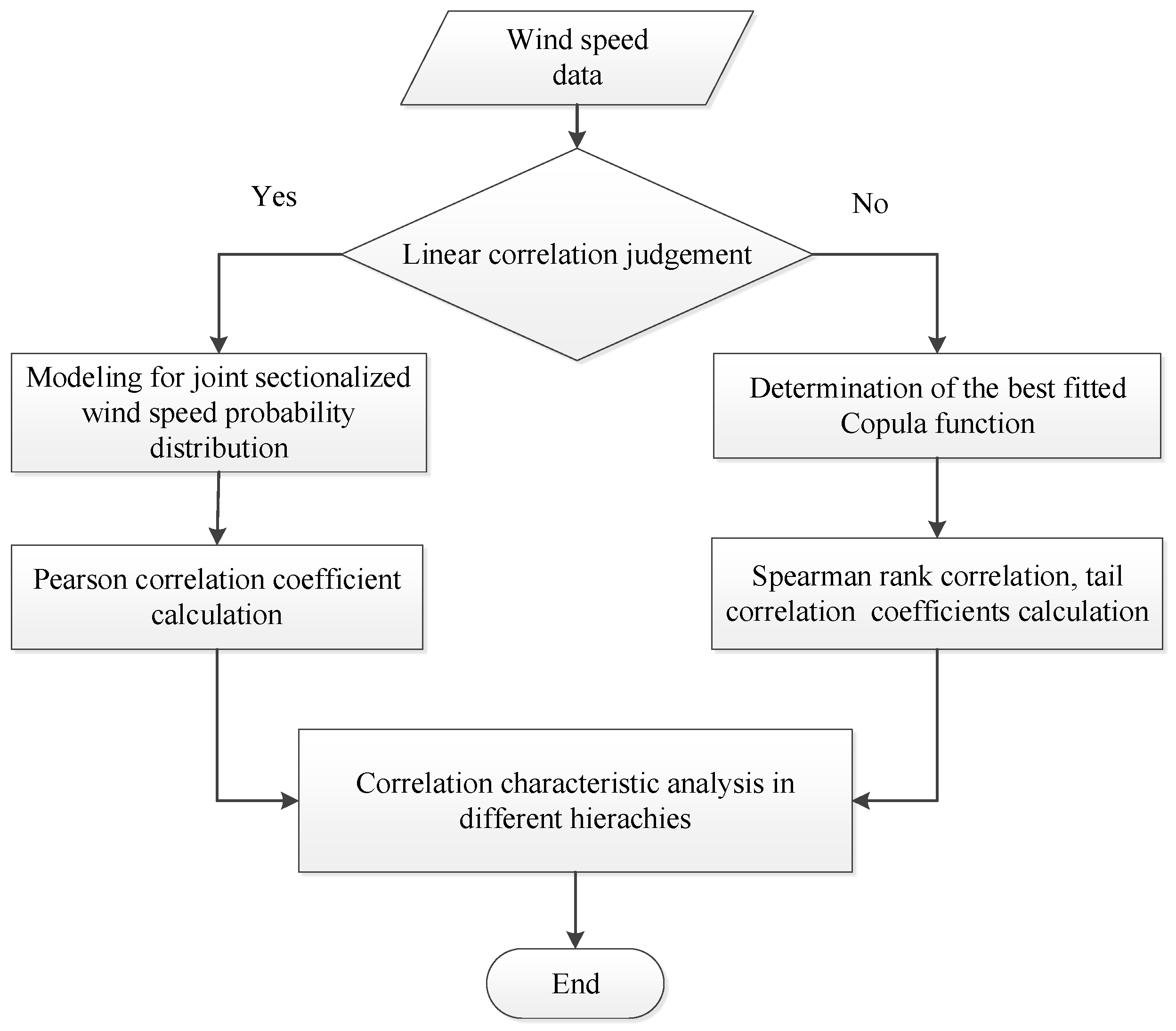
This paper addresses the analysis for correlation characteristics of wind speed in different geographical hierarchies that is, among wind turbines, within the wind farm and its wind turbines, and among wind farms. According to the linear or nonlinear correlation condition in each geographical hierarchy, the use of the Pearson coefficient for linear correlations, and Spearman and tail coefficients for nonlinear correlations were judged, respectively. In this paper, the proposed approach is to analyze the correlation characteristics of wind speed quantitatively and qualitatively based on data from the Wind Speed Dataset of the Gansu Wind Power Technology Center, China. The correlation characteristic analysis in different geographical hierarchies will provide detailed correlation information to improve the accuracy of wind speed or power prediction. It is implemented to evaluate the wind unit siting and wind farm planning, especially for China’s concentrated wind power integration. They is certainly high interest in production probability simulation, which contributes to power system planning and risk assessments. We note that while in this work the proposed approach is applied to the Gansu Wind Power Base, it can be easily extended to other cases in different regions.

The remainder of the paper is organized as follows: Section 2 introduces the linear correlation analysis including joint sectionalized wind speed probability modeling and linear correlation coefficient for correlation measurement. In addition, nonlinear correlation analysis including Copula theory and its nonlinear correlation coefficients are given in Section 3. The proposed methodology for analysis of the correlation characteristics of wind speed in different hierarchies is described in Section 4. Case studies on the correlation characteristics of wind speed among wind turbines, among wind farm and its wind turbines, and among wind farms are discussed in Section 5. Conclusions are given in Section 6.

2. Linear Correlation Analysis

Correlations can be classified as linear correlations and nonlinear correlations. Linear correlations, which refer to a straight line correlation between two variables, characterize the degree of correlation to which larger wind speed x values go with larger speed y values and smaller x values go with smaller y values in the paired wind data sets. In this section, the method to establish a joint sectionalized wind speed probability distribution will be introduced. The joint sectionalized probability distribution is appropriate for linear correlations in a qualitative way. Then, the Pearson coefficient that can be used to quantitatively measure the linear correlation between the individual values of wind speed series at different locations.

2.1. Modeling for Joint Sectionalized Wind Speed Probability Distribution

At the beginning of a correlation analysis, it is necessary to qualitatively identify whether the correlation is linear or not. Thus historical wind speeds are treated by dividing wind speeds into several sections, which could provide an efficient way to avoid using huge amounts of measured wind speed data. Based on the segmentation, a joint sectionalized wind speed probability distribution at different locations (e.g., in wind turbines or wind farms) can be established. Furthermore, correlation of wind speed among locations can be analyzed quantitatively.

2.1.1. Wind Speed Sectionalizing

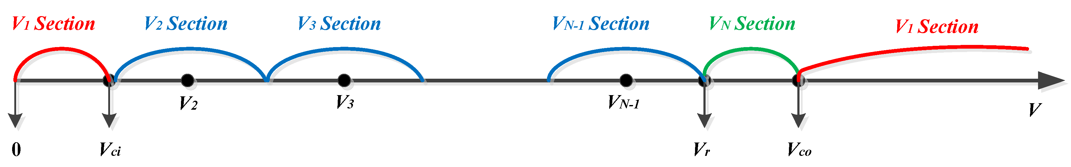
Values of wind speed series at one location are divided into N sections within the wind speed variation range, so that N sectionalized wind speed points are obtained in the middle of each section. The wind speed values are then classified into the section in which their nearest sectionalized point are located. Figure 1 illustrates the sectionalizing process.

As the wind power is zero when the wind speed is below the cut-in wind speed or above the cut-out wind speed, wind speed values within these ranges are regarded to be the equivalent cut-in wind speed value, marked as the first sectionalized wind speed value:

$$V_1=V_{ci},$$

(1)

where V₁ represents the first sectionalized wind speed value; and V_ci represents the cut-in wind speed.

When the wind speed value is between rated wind speed and cut-out wind speed, the wind power reaches to the rated value. Thus, the N_th sectionalized wind speed value can be marked as:

$$V_N=V_r,$$

(2)

where V_N represents the N_th sectionalized value, and V_r represents the rated wind speed.

When the wind speed is between the cut-in wind speed and rated wind speed, wind power varies with wind speed. Therefore, other sectionalized wind speed points are:

$$V_{step}=\frac{(V_r-V_{ci})}{N-2},$$

(3)

$$V_i=V_{ci}+\frac{2i-3}{2}{V}_{step},i=2,3,\mathrm{...},N-1,$$

(4)

where V_step represents the wind speed interval between two adjacent sectionalized wind speed points; and V_i represents the i_th sectionalized points.

2.1.2. Joint Sectionalized Probability Distribution of Wind Speeds

After sectionalizing the wind speed, the probability of the wind speeds divided into the corresponding section is obtained. By establishing the joint probability of wind speeds at different locations, correlation of wind speed among those locations can be intuitively described in an efficient way. 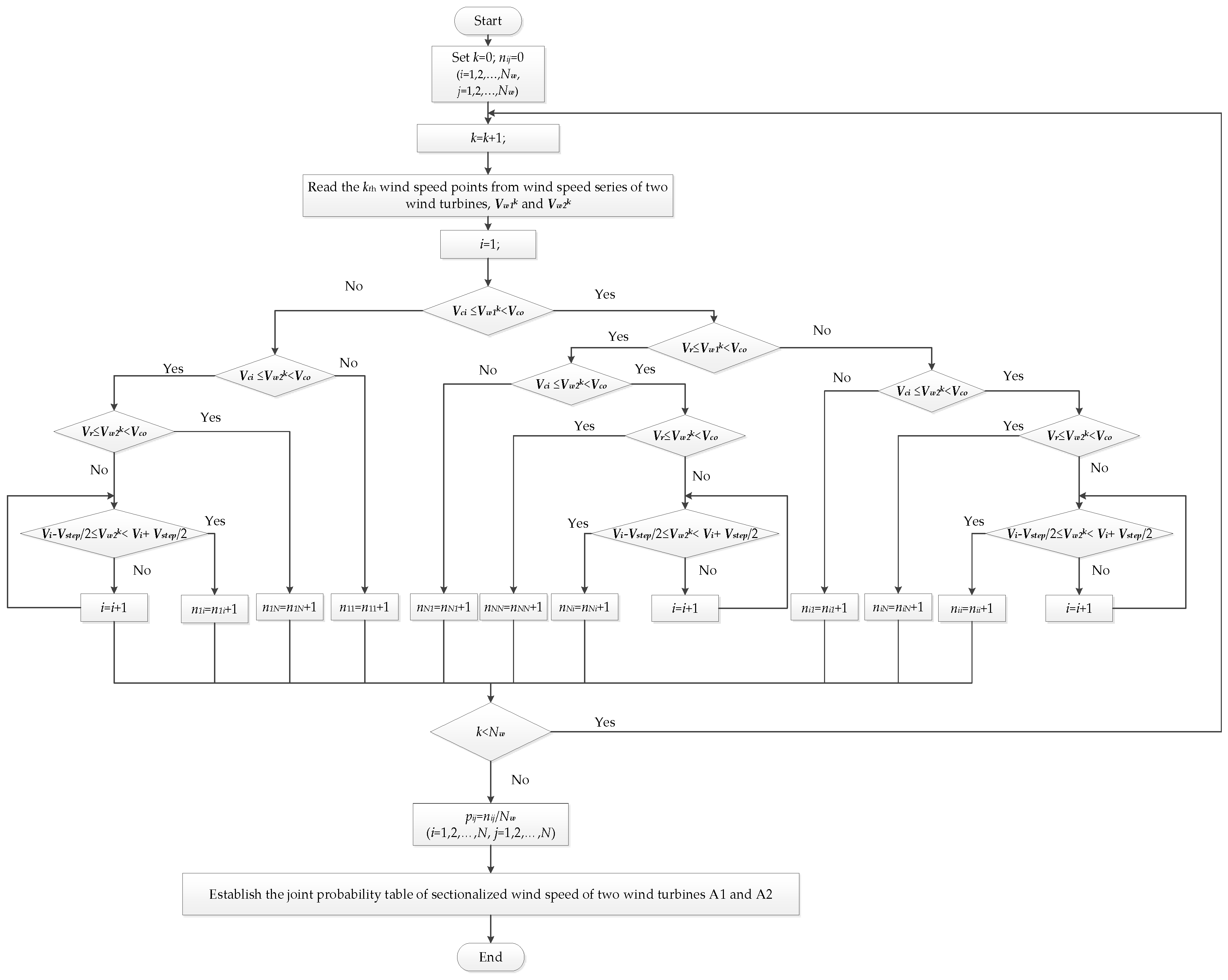Suppose that one wishes to model the joint sectionalized wind speed probability of two turbines A1 and A2, each with one year of N_w measured wind speed points. Based on the sectionalized wind speeds of each wind turbine, the joint sectionalized wind speed probability can be modeled as Figure 2 shows. The detailed steps of modeling are as follows:

Step 1:

Set k = 0, n_ij = 0 (i = 1, 2, …, N_w, j = 1, 2, …, N_w);

Step 2:

k = k + 1. Read the k_th wind speed point from wind speed series of two wind turbines, V_w1^k and V_w2^k;

Step 3:

If V_w1^k < V_ci or V_w1^k ≥ V_co, then V_w1^k equivalently locates on the sectionalized point V₁,

Step 3.1:

If V_w2^k < V_ci or V_w2^k ≥ V_co, then V_w2^k equivalently locates on the sectionalized point V₁, then n₁₁ = n₁₁ + 1;

Step 3.2:

If V_r ≤ V_w2^k < V_co, V_w2^k equivalently locates on the sectionalized point V_N, then n_1N = n_1N + 1;

Step 3.3:

If V_i − V_step/2 ≤ V_w2^k < V_i + V_step/2, V_w2^k equivalently locates on the sectionalized point V_i, then n_1i = n_1i + 1;

Step 4:

If V_r ≤ V_w1^k < V_co, then V_w2^k equivalently locates on the sectionalized point V_N,

Step 4.1:

If V_w2^k < V_ci or V_w2^k ≥ V_co, V_w2^k equivalently locates on the sectionalized point V₁, then n_N1 = n_N1 + 1;

Step 4.2:

If V_r ≤ V_w2^k < V_co, V_w2^k equivalently locates on the sectionalized point V_N, then n_NN = n_NN + 1;

Step 4.3:

If V_i − V_step/2 ≤ V_w2^k < V_i + V_step/2, V_w2^k equivalently locates on the sectionalized point V_i, then n_Ni = n_Ni + 1;

Step 5:

If V_i − V_step/2 ≤ V_w1^k < V_i + V_step/2, then V_w2^k equivalently locates on the sectionalized point V_i,

Step 5.1:

If V_w2^k < V_ci or V_w2^k ≥ V_co, V_w2^k equivalently locates on the sectionalized point V₁, then n_i1 = n_i1 + 1;

Step 5.2:

If V_r ≤ V_w2^k < V_co, V_w2^k equivalently locates on the sectionalized point V_N, then n_iN = n_iN + 1;

Step 5.3:

If V_i − V_step/2 ≤ V_w2^k < V_i + V_step/2, V_w2^k equivalently locates on the sectionalized point V_i, then n_ii = n_ii + 1;

Step 6:

If k < N_w, go to Step 2; otherwise, go to Step 7;

Step 7:

The joint probability of sectionalized wind speed is p_ij = $\frac{n_{ij}}{N_w}$ (i = 1, 2, …, Nw, j = 1, 2, …, Nw);

Step 8:

Establish the joint probability table of sectionalized wind speed of two wind turbines A1 and A2, shown as

Table 1. Joint probability of sectionalized wind speed of two wind turbines.

	Wind Speed of A1	V1	V2	....	VN−1	VN
Wind Speed of A2
V1		p11	p11	…	p1,N−1	p1,N
V2		p21	p22	…	p2,N−1	p2,N
...		...	...	...	...	...
VN−1		pN−1,1	pN−1,2	…	pN−1,N−1	pN−1,N
VN		pN,1	pN,2	…	pN,N−1	pN,N1

.

Joint probabilities on the diagonal line in the table show the possibility of the same contemporaneous wind speed values of two wind turbines, providing a qualitative way to judge whether wind speed relationship of two turbines is linear correlation or not. The method for modeling the joint probability of sectionalized wind speed of different wind turbines can also be applied to the analysis for wind farms.

2.2. Linear Correlation Coefficient

The Pearson correlation coefficient is generally used to measure the linear dependency of random variables. Let X, Y be two random variables with their expectation E(X) and E(Y). Suppose variance D(X) > 0 and D(Y) > 0, Pearson correlation coefficient r is defined as [19]:

$$r=\frac{\mathrm{cov}(X,Y)}{\sqrt{D(X)}\sqrt{D(Y)}},$$

(5)

$$\mathrm{cov}(X,Y)=E\{[X-E(X)][Y-E(Y)]\},$$

(6)

$$D(X)=E{[X-E(X)]}^2=E(X^2)-{[E(X)]}^2$$

(7)

$$D(Y)=E{[Y-E(Y)]}^2=E(Y^2)-{[E(Y)]}^2$$

(8)

where cov(X,Y) is covariance of X and Y.

The Pearson coefficient r is between −1 and 1. The absolute value of correlation coefficient r measures the strength of the linear relationship between X and Y. The value of |r| equal to 1 means that there is a perfect linear relation. The linear correlation of two variables gets stronger when |r| gets close to 1; and they have no relation when r is 0. When r > 0 we say that the data pairs are positively correlated; and when r < 0 we say that they are negatively correlated.

Though Pearson coefficients are often straightforward to calculate, they cannot properly describe correlation of variables with heavy-tailed distribution, for example, observations for wind speed. Besides, independence of two random variables implies they are uncorrelated (r(X,Y) = 0) but a zero correlation does not in general imply independence. Only in the case of the multivariate normal distribution is it permissible to interpret uncorrelated as implying independence. Besides, it fails to deal with nonlinear correlation problems due to its limited properties and conditions.

3. Nonlinear Correlation Analysis

Joint sectionalized wind speed probability distributions provide an efficient way to observe the linear relationship between wind turbines (farms) but fails to indicate nonlinear relationship and their dependence structure. Copula theory is generally utilized to analyze the nonlinear correlation for wind speed and wind power. This section will introduce Copula functions and choose the best-fitted Copula function to best fit the joint wind speed distribution of different locations. The Spearman rank correlation and tail correlation coefficients will be given as quantitative measurements of nonlinear relationship between wind speed series at different locations

3.1. Copula Function

Copula function is used extensively to get the joint probabilistic distribution of random variables, characterizing the non-normal nature of a single random variable [20]. By connecting the marginal distribution of each variable function into a joint distribution function, it is able to capture the nonlinear, asymmetric and the upper and lower tail correlation using correlation indicators that we will introduce in the next subsection.

Copulas are multivariate uniform distributions. They represent a way of trying to extract the dependence structure from the joint distribution function and to separate dependence and marginal behavior. Suppose that we model the joint cumulative distribution function of wind speed at different locations with specified marginal cumulative distribution functions (e.g., Weibull). Let random variables represent contemporaneous wind speed of n locations, and they are represented by x_i (i = 1, …, n). The cumulative distribution function of x_i can be connected using copula function to get the joint distribution, which is formulated as:

$$F(x_1,\cdots ,x_n)=C(F_1(x_1),\cdots ,F_n(x_n)),$$

(9)

where F₁, …, F_n, are the marginals; C($·$) is the copula function of F_i; and F($·$) is the joint distribution of x₁, …, x_n. Then the joint distribution density function f($·$) is formulated as follows:

$$f(x_1,\cdots ,x_n)=\frac{\partial C({\mu }_1,{\mu }_2,\cdots ,{\mu }_n)}{\partial {\mu }_1\partial {\mu }_2\cdots \partial {\mu }_n}{\displaystyle \prod _{i=1}^n\frac{\partial F_i(x_i)}{\partial x_i}},$$

(10)

where μ_i is F_i(x_i) for simplicity. A Copula gives a model for the dependence structure that reflects more detailed knowledge of wind speed variables.

There are many candidate Copula functions in different Copula families, such as elliptical Copulas (Gaussian and t) and Archimedean Copulas (Gumbel, Clayton and Frank) [21]. Different tail behaviors in distribution are described in those Copulas. Gaussian_Copula, t_Copula and Frank_Copula functions have symmetric tails but cannot capture the features of asymmetric tail dependence; Gumbel_Copula and Clayton_Copula functions have asymmetric tails with capability of capturing the asymmetric tail dependence.

In terms of study on wind speed, the tail features in wind speed distributions are different with respect to different locations or geographical regions, so the fitted-best Copula is needed to be selected in a proper manner to fit the wind speed data with its features. A proper description for tail features can improve the accuracy in the wind speed-forecasting model. The method for choosing the fitted-best Copula will be introduced in the following section.

3.2. Determincation of Copula Types under Nonlinear Correlation Condition

In Copula analysis, it is necessary to fit a joint Copula distribution function and evaluate the goodness-of-fit of data to the models by selecting a proper Copula function from a Copula family including Gauss, t, Gumbel, Frank, Clayton, etc. The steps involved in determining the copula function to best fit the joint wind speed distribution of two locations are as follows:

Step 1:

Use the Kernel density estimation method to calculate the marginal cumulative distribution functions of wind speed at each location. Then transform the marginal cumulative distribution functions into uniform distributions by cumulative integration [22].

Step 2:

Construct the joint Copula functions of wind speed at different locations. Unknown parameters of the joint Copula functions are estimated by the maximum likelihood estimation method.

Step 3:

The empirical joint Copula distribution function of wind speed is calculated [23]. Then calculate Euclidean distances of the empirical Copula function with each obtained copula distribution. Moreover, the Copula function with its minimum Euclidean distance among Copula families best fits the actual correlation of wind speed at different locations.

3.3. Nonlinear Correlation Coefficients

Previous defects of linear Pearson coefficient can be overcome by nonlinear correlation coefficients such as the Spearman rank coefficient and tail correlation coefficients [23]. These coefficients based on Copula functions can capture the consistence of variation of observations to measure nonlinear correlation of random variables.

3.3.1. Spearman Rank Correlation Coefficient

The consistence of wind speed series variations in time at locations could be measured by the Spearman rank correlation coefficient. Suppose that two-dimensional vectors (X,Y) are independent random variables having common density function. In terms of paired values (X₁,Y₁), (X₂,Y₂) and (X₃,Y₃), Spearman rank correlation coefficient ρ is defined as follows:

$$\rho =3\{\mathrm{P}[(X_1-X_2)(Y_1-Y_3)>0]-\mathrm{P}[(X_1-X_2)(Y_1-Y_3)<0]\},$$

(11)

The Spearman rank correlation coefficient is the multiple of probability difference between concordance and discordance. It is used to measure whether two variables vary in trend consistently or not. The Spearman coefficient based on Copula function can be formulated as:

$$\rho =12{\displaystyle {\int }_0^1{\displaystyle {\int }_0^1\mu \upsilon \mathrm{d}C(\mu ,\upsilon )}}-3,$$

(12)

where μ and ν are marginal distribution of continuous random variables vectors (X,Y) respectively, in the Copula function C(μ,ν). Note that two marginal distributions of (X,Y) are both a uniform distribution U(0,1). The Spearman rank correlation coefficient value is between −1 and +1. The sign of ρ gives the direction of the relation. It is positive when smaller Y value tends to go with X value getting smaller and larger Y value with X value getting larger; and it is negative when larger Y value tends to go with X value getting smaller and smaller Y value with larger value.

3.3.2. Tail Correlation Coefficients

In the wind speed correlation analysis, tail correlation must considered. As wind speed is related to the wind power output, the tail correlation coefficient shows the degree of influence of wind speed at one location on the wind speed at other locations when the speed rises or declines sharply. An extreme wind speed value may cause a significant impact on wind speed and power forecast.

The Tail correlation coefficient λ consists of an upper tail correlation coefficient λ^up and lower tail correlation coefficient λ^lo. Let F(x) and G(y) be marginal distributions of continuous random vectors (X,Y) respectively, the upper and lower tail correlation coefficients are defined as:

$${\lambda }^{up}=\underset{\mu \to 1^{-}}{\lim }\mathrm{P}[Y>G^{-1}(\mu )|X>F^{-1}(\mu )],$$

(13)

$${\lambda }^{lo}=\underset{\mu \to 0^{+}}{\lim }\mathrm{P}[Y<G^{-1}(\mu )|X<F^{-1}(\mu )],$$

(14)

The tail correlation relates to the dependence of extreme values, and depends mainly on the tails. It shows how one of the two variables value is dependent on the other when the other variable value is larger or less than a threshold value. Values of λ^up and λ^lo are between 0 and 1. If λ^up (or λ^lo) exists and is positive, X and Y are dependent in upper (or lower) tail. Upper and lower tail correlation coefficient λ^up and λ^lo based on Copula function can be formulated as follows:

$${\lambda }^{up}=\underset{\mu \to 1^{-}}{\lim }\frac{1-2\mu +C(\mu ,\mu )}{1-\mu },$$

(15)

$${\lambda }^{lo}=\underset{\mu \to 0^{+}}{\lim }\frac{C(\mu ,\mu )}{\mu },$$

(16)

where μ and ν are marginal distribution of continuous random variables vectors (X,Y) respectively in the Copula function C($·$). Note that two marginal distributions of (X,Y) are both a uniform distribution U(0,1).

4. Methodology of Correlation Characteristic Analysis in Different Geographical Hierarchies

As geographical diversity affects wind speed uncertainty and variability, the correlation characteristics are different in the variety of distances and terrain where wind turbines and wind farms are located. In this section, the proposed method for correlation characteristics analysis in different geographical hierarchies will be introduced based on the model and method introduced in Section 2 and Section 3.

4.1. Judgement of Linear or Nonlinear Correlation

Before correlation analysis, whether there is a linear or nonlinear correlation should be judged in each geographical hierarchy. To improve analysis efficiency, a scatter diagram, which portrays a data set of paired values on a two-dimensional graph with the x-axis representing the x values of the data and the y-axis representing the y values, is a straightforward and intuitive way to present a linear correlation. Here we utilize both the scatter diagram and the joint probability table of sectionalized wind speeds as a combined way to qualitatively judge whether the correlation is linear or not.

When the wind speed correlation is linear, there is a upward straight line relation between the paired data such that large wind speed y values are attached to large wind speed x values as shown in Figure 3a, or a downward straight line relation that large wind speed y values are attached to small wind speed x values. Meanwhile, large values of joint probability are almost on the diagonal line in the joint sectionalized wind speed table. Otherwise, when the paired data values scatter randomly in the graph as shown in Figure 3b and large values of joint probability are not on the diagonal line of the sectionalized wind speed table, there may be a nonlinear correlation or no correlation between them. In this situation, the Copula functions mentioned in the previous section can be adopted to capture them.

4.2. Methods of Correlation Characteristic Analysis for Wind Speed in Different Geographical Hierachies

As mentioned above, linear wind speed correlation should be firstly judged using the scatter diagram. The joint sectionalized wind speed probability is then modeled to describe the wind speed correlation qualitatively. If the correlation of wind speed between locations (in wind turbines or wind farms) is linear, a Pearson coefficient is calculated to describe the wind speed linear correlation quantitatively. Otherwise, the best-fitted Copula function is constructed, and the Spearman rank correlation coefficient as well as the tail correlation coefficient is calculated to measure the wind speed nonlinear correlation.

To sum up, analysis of the correlation characteristics of wind speed in different geographical hierarchies is subsequently performed based on the model and method above. Figure 4 indicates the flow chart for this process, and detailed procedures will be introduced in following subsections.

4.2.1. Analysis on the Correlation Characteristics of Wind Speed among Multiple Wind Turbines

The wind speed of each wind turbine may vary differently due to the variety of terrain that wind turbines cover. For instance, the wind turbine downstream experiences a similar wind as upstream for certain wind directions but with a time delay. The goal for analyzing the correlation characteristics of wind speed among wind turbines is to provide useful correlation information for wind turbine layout and wind farm siting planning.

To analyze the temporal-geographical correlation of wind speed among wind turbines, the wind speeds series of any two wind turbines in a certain period are treated by shifting several time intervals from wind speed series of the one wind turbine while keeping those of the other unchanged. Figure 5 shows the wind speed series of two wind turbines before and after a shifting certain time interval.

According to their linear or nonlinear correlation that was previously judged, the corresponding correlation coefficients are calculated with respect to various shifted time intervals of the two wind speed series. The shifted time interval value varies from the lagging time difference to the leading time difference. Then draw a plot with the x-axis representing the time difference values from the negative (lagging) to the positive (leading) and the y-axis representing the correlation coefficient values to examine the distances between the target wind turbines. It also investigates the upstream and downstream relationship between wind turbines.

In addition, the correlation coefficient values of every two wind turbines in the same wind farm are calculated. The mathematical relationship of distance and coefficient value is then fitted to grasp the variation rule of correlation with the distance among wind turbines.

4.2.2. Analysis on Correlation Characteristics of Wind Speed among a Wind Farm and Its Wind Turbines

The temporal correlation characteristics of wind speed among a wind farm and its wind turbines are analyzed on short and long-time scales. Generally, the wind speed of a wind farm is the average values of all the wind turbines in this wind farm, which reflects the overall wind speed variation over it. Through the investigation on the correlation characteristics of wind speed in this geographical hierarchy, the internal wind speed variation law in the wind farm can be revealed and reflect the features of wind speed variation on different time scales.

Historical wind speed series are firstly selected every 0.5 h, 1 h for the short time scale and 6 h, 12 h for the long time scale. Then correlation coefficient values describing the relationship of wind speed in wind farm and its turbine are calculated in each time interval to obtain the probability density distribution. We compare the probability density distributions of correlation coefficients in different time intervals to analyze the impact of wind speed in wind turbines on its belonging wind farm.

4.2.3. Analysis on Correlation Characteristics of Wind Speed among Multiple Wind Farms

Several previous studies showed that temporal and geographical correlation among wind farms may not be as strong as that among wind turbines because wind farms span a larger geographical area than wind turbines. Therefore, neither linear correlation analysis nor general Copula functions such as normal_Copula and t_Copula can capture well their relationship. Moreover, not only their dependence structure but also the tail correlation should be modeled in an appropriate way, so that the dependence of wind speed among wind farms can be completely represented in any model. Based on the method for choosing the best-fitted joint distribution function introduced in the previous section, here we construct the best-fitted Copula function from Archimedean Copulas and calculate the correlation coefficients to analyze the dependence structure and tail correlation of the wind speed series among multiple wind farms. Based on the correlation characteristics of wind speed that can be transformed to wind power with the wind power curve, an improvement in accuracy of wind power forecasting can be achieved with detailed correlation information, which is of significance to power system analysis and security assessment.

5. Case Study

5.1. Case Background

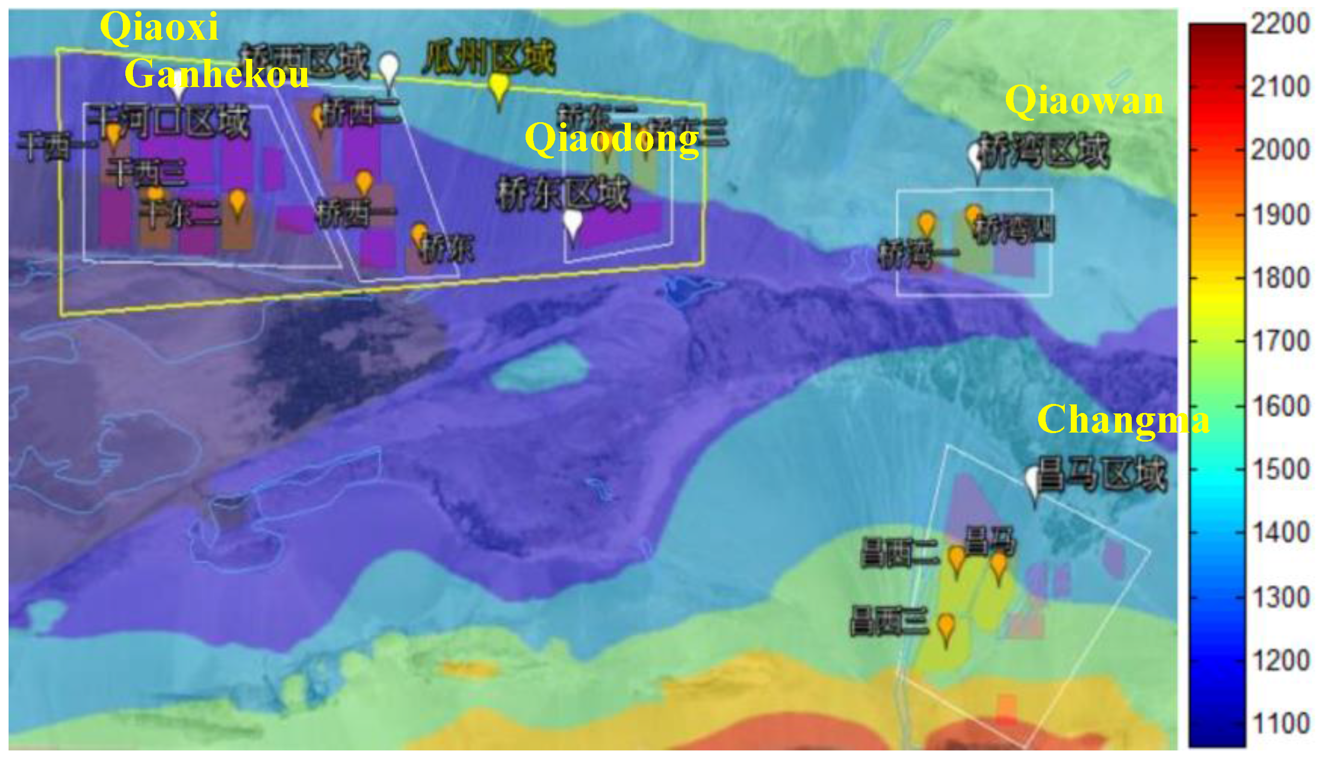
Jiuquan in northwest China, is under construction for the biggest 10 GW wind power base in Gansu Province, which is known for its abundant wind energy resources. Wind energies are concentrated in this area due to the well-known Hexi Corridor with its 160 km length and 100 km width. As shown in Figure 6, the Gansu wind area is divided into five regions including Ganhekou, Qiaoxi, Qiaodong, Qiaowan and Changma all located in the Jiuquan Wind Power Base. The wind characteristics in Ganhekou, Qiaoxi and Qiaodong regions are similar due to their similar terrains in the north, while the winds are different in the Changma region located in the southeast. In this paper, the wind speed correlation characteristics between the Qiaodong and Changma regions are investigated as a typical case.

To explore the correlation under different hierarchies, that is among wind turbines, among the farm and its wind turbines, and among wind farms, wind speed measurements characterizing farms located in each of the two geographical regions of interest as well as turbines located in each of farms of interest are clearly needed.

For the needs of the present paper, the wind farm Qiaodong II with its 134 wind turbines (Qiaodong Region) and Changxi I (Changma Region) with its 65 wind turbines are considered and summarized in

Table 2. Gansu wind farms in investigated regions.

Wind Farm	Wind Turbine Numbers	Cut-in Wind Speed (m/s)	Rated Wind Speed (m/s)	Cut-out Wind Speed (m/s)	Periods	Time Interval (min)
Qiaodong II	134	3.0	11.5	25	2015.01.01–2015.12.30	5
Changxi I	98	3.0	10.5	20	2015.01.01–2015.12.30	5

. In this paper, wind speed series measured every 5 min were provided.

5.2. Correlation Characteristics of Wind Speed among Wind Turbines

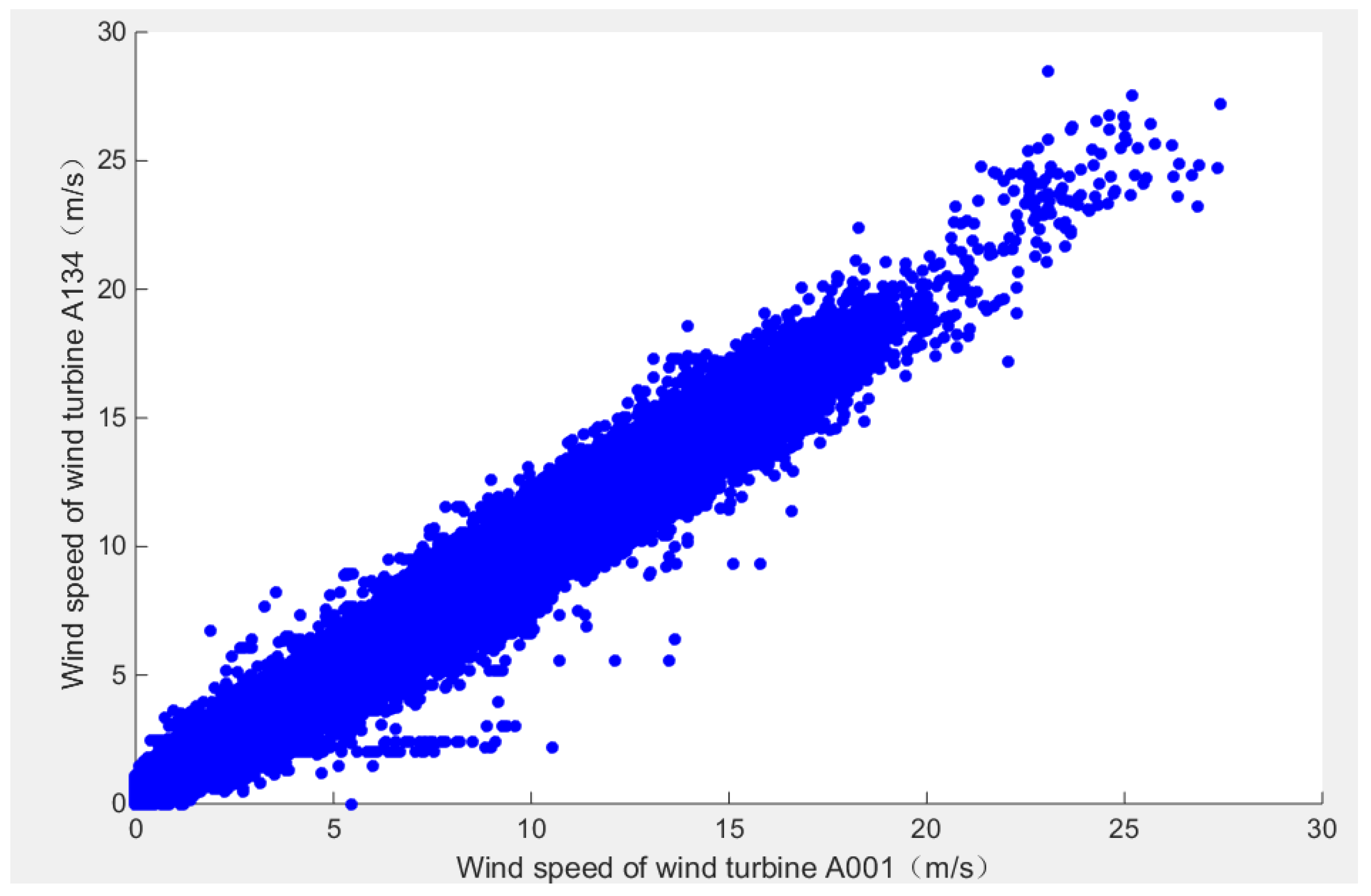
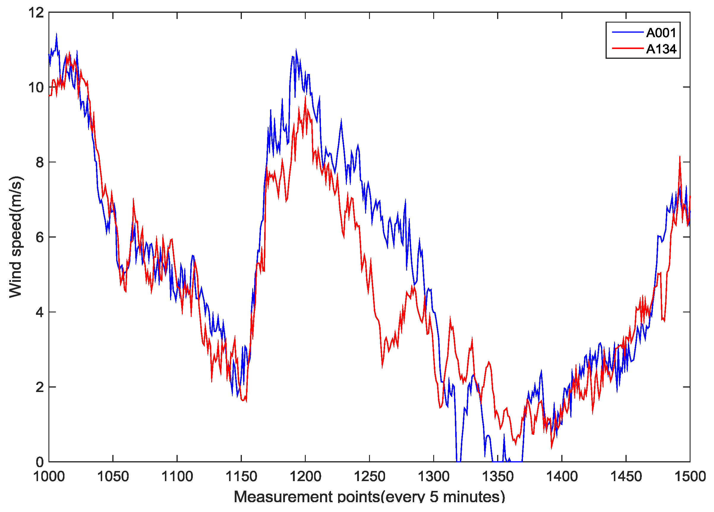
In the goal of exploration of the correlation characteristics of wind speed among wind turbines located in the same geographical region, a pair of wind turbines A001 and A134, both located in wind farm Qiaodong II were taken as an example using the proposed method.

Using wind speed series in time ranging from 2015.1.1 to 2015.12.30, the linear correlation of wind speed between A001 and A134 is clearly shown in Figure 7. It shows that points of wind speed are observed to scatter near the straight line. After sectionalizing the wind speed series of each wind turbine, the joint probability of sectionalized wind speed of two turbines was established as

Table 3. Joint probability of discrete wind speeds of wind turbines A001 and A134.

	Wind Speed of A001 (m/s)	≤3	3.5	4.5	5.5	6.5	7.5	8.5	9.5	10.5	≥11.5
Wind Speed of A134 (m/s)
≤3		0.3967	0.0633	0.0025	0.0001	0.0087	0.0000	0.0000	0.0000	0.0000	0.0001
3.5		0.0701	0.0753	0.0117	0.0003	0.0001	0.0000	0.0000	0.0000	0.0000	0.0000
4.5		0.0083	0.0243	0.0612	0.0104	0.0004	0.0001	0.0000	0.0000	0.0000	0.0000
5.5		0.0007	0.0023	0.0233	0.0511	0.0126	0.0005	0.0001	0.0000	0.0000	0.0000
6.5		0.0002	0.0001	0.0021	0.0436	0.0475	0.0126	0.0009	0.0001	0.0000	0.0000
7.5		0.0001	0.0000	0.0003	0.0020	0.0167	0.0365	0.0120	0.0011	0.0001	0.0000
8.5		0.0001	0.0000	0.0000	0.0003	0.0022	0.0134	0.0304	0.0115	0.0011	0.0002
9.5		0.0000	0.0000	0.0000	0.0001	0.0003	0.0016	0.0124	0.0285	0.0134	0.0018
10.5		0.0000	0.0000	0.0000	0.0000	0.0000	0.0001	0.0015	0.0119	0.0255	0.0158
≥11.5		0.1082	0.1081	0.1081	0.1081	0.1081	0.1081	0.1082	0.1097	0.1189	0.2574

The joint probability values on the diagonal line represent the possibility of identical sectionalized wind speeds of two turbines at the same time point.

, further describing their linear correlation in quantities. The number of sectionalized joints of wind speed was set as 10 according to practical experience.

It is observed that the large joint probability values (marked in blue) are almost on the diagonal line, which indicates that the instantaneous wind speeds of A001 and A134 are close. In addition, the strong linear correlation of wind speed between A001 and A134 is shown in Figure 7 and Table 3, apparently because they are adjacent in geographical locations in the same wind farm sharing a similar wind regime. Thus, their linear correlation characteristics can be expressed by a Pearson correlation calculation.

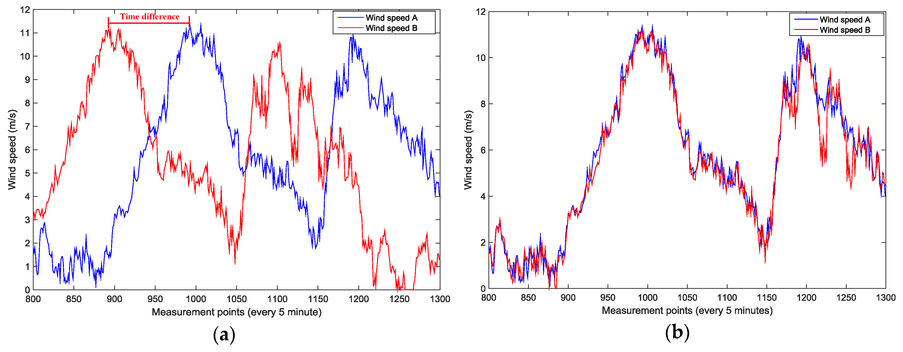
As each wind turbine is at a distance ranging from 200 m to 10 km from others in the Qiaodong II wind farm, the wind speed of each wind turbine may vary differently due to the distance. To analyze the temporal-geographical correlation of wind speed between wind turbines, the wind speeds in time series of two wind turbines in a certain period were treated by shifting several time intervals from the wind speed series of wind turbine A001 and keeping that of A134 unchanged. The Pearson coefficient, which tests the correlation of the two treated wind speed series, was then calculated to examine the distance relationship between A001 and A134. The original measured wind speed series of A001 and A134 in a certain period is shown in Figure 8, which describes a time difference between two wind speeds series.

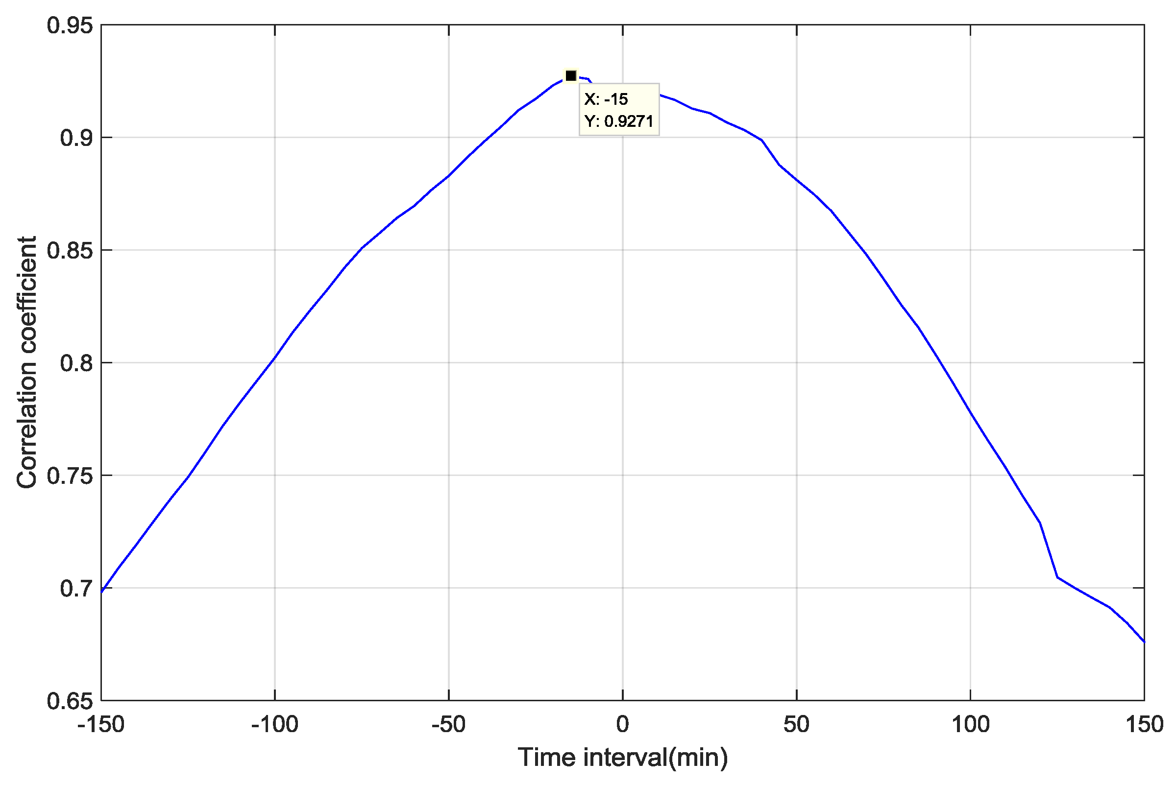
Then the Pearson coefficients were calculated in different shifted time intervals. Figure 9 depicts the variation of correlation coefficient values corresponding to different shifted intervals. The shifted time of A001 wind speed series ranges from −150 min to +150 min. Note that “–“ means the shifted wind speed series of A001 is lagging behind that of A134 while “+” means the shifted series of A001 is ahead of that of A134. The peak value of the Pearson coefficient is reached at 0.9271 when the time intervals of A001 are shifted backward by 15 min, which means that the two have a strong correlation after time shifting. The time difference “15 min” can be intuitively explained by their geographical distance. Indeed, the distance where the wind at a mean speed (5 m/s) goes from A134 to A001 lasting for 15 min is exactly examined to be their actual distance (4–5 km), which indicates A134 was upstream of A001 during that period.

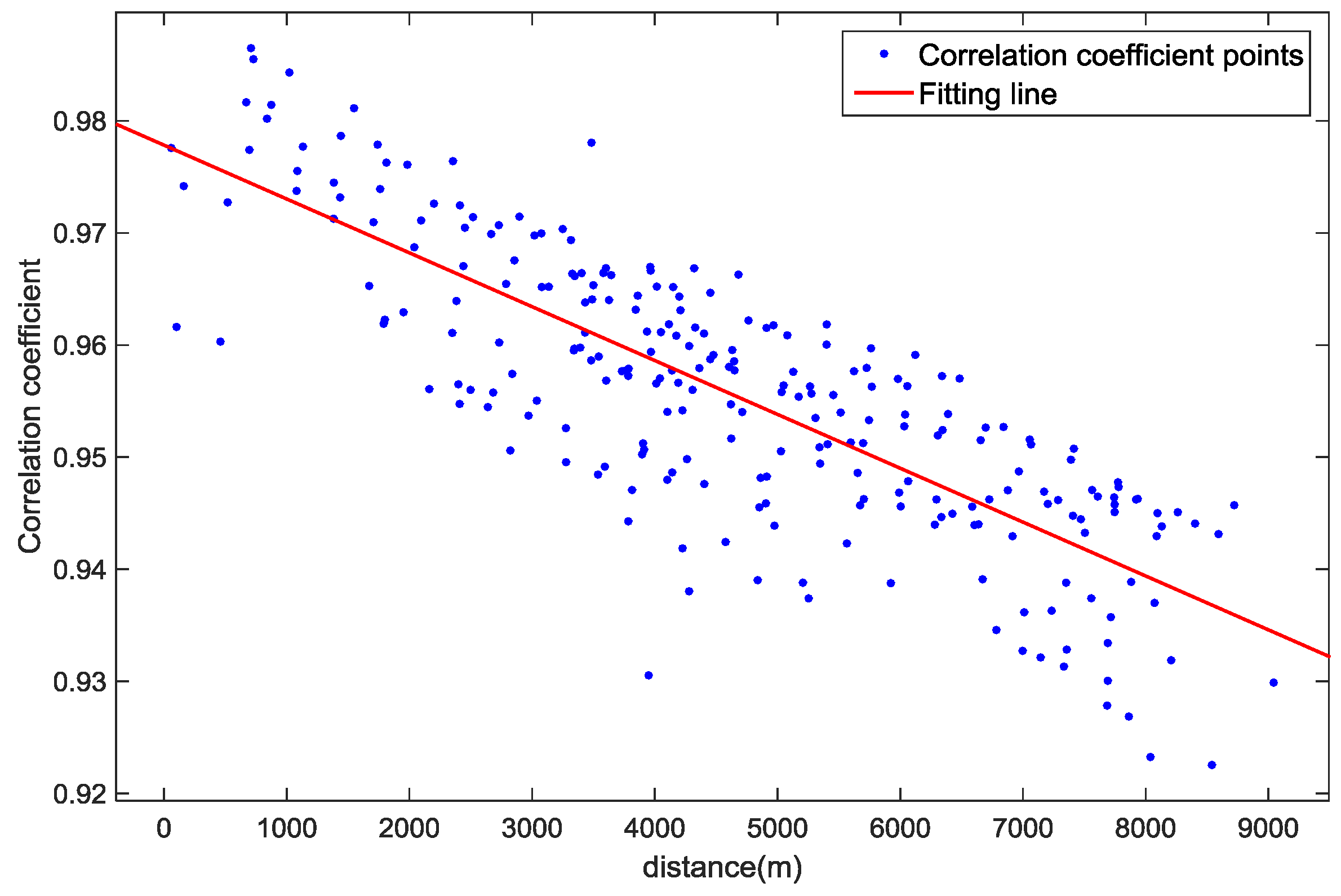
Wind speeds of 134 wind turbines for one year in the Qiaodong II wind farm were treated by calculating the correlation coefficients between any two turbines. Figure 10 describes a downtrend of correlation coefficient values as the distance of two corresponding turbines is increasing. It is observed that there is a strong correlation between any two wind turbines in the same wind farm shown in Figure 10, where all the correlation coefficients are higher than 0.9 even if the furthest distance is 9 km. By linear fitting, the linear relationship between the Pearson coefficients and geographical distance is as follows:

$$S=-4.803\times {10}^{-6}d+0.9798$$

(17)

where d represents the distance between two wind turbines; S represents the correlation coefficient value; and the goodness of fit is 0.6544. This knowledge leads to a recommendation to enlarge the balancing areas, and to construct transmission paths in diverse locations.

The investigation for correlation characteristics in time and geography can be applied to evaluate the wind unit siting and wind farm planning, which is of significance in practice and engineering.

5.3. Correlation Characteristics of Wind Speed among a Wind Farm and Its Wind Turbines

The correlation characteristics of wind speed among a wind farm and its wind turbines on short and long time scales were investigated with one year of collected wind speeds in a wind farm. We take the Qiaodong II wind farm and its 134 wind turbines as an study example. Periods of experimental wind speed in time series were considered as 0.5 h, 1 h for the short time scale and 6 h, 12 h for the long time scale.

To reflect the overall wind speed variation in the Qiaodong II area, the wind speed of the wind farm was treated by averaging wind speeds of all wind turbines in the same wind farm. As demonstrated in Section 4.2, wind turbines in the same wind farm have strong correlations with each other, so the Pearson coefficients were calculated at 0.5 h, 1 h, 6 h and 12 h time intervals, respectively, based on the wind speed series of the Qiaodong II wind farm and its wind turbines.

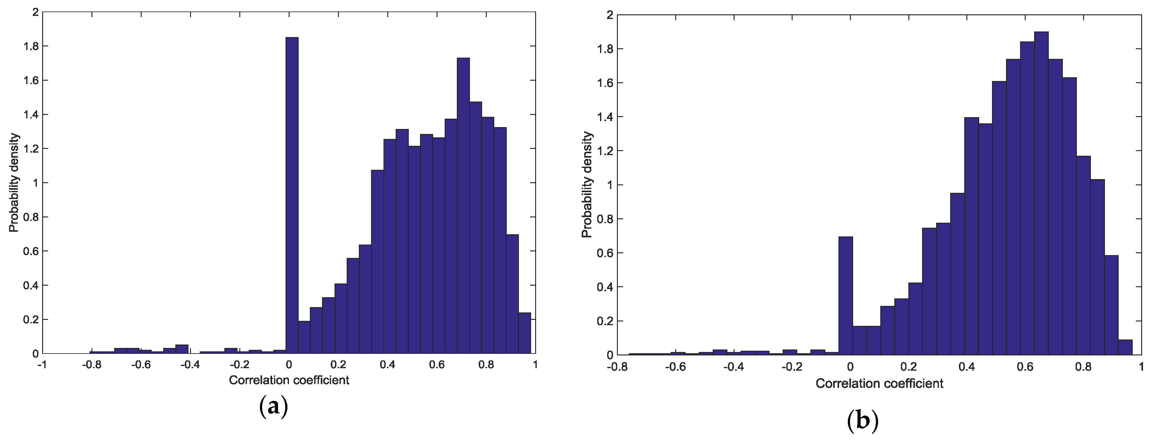
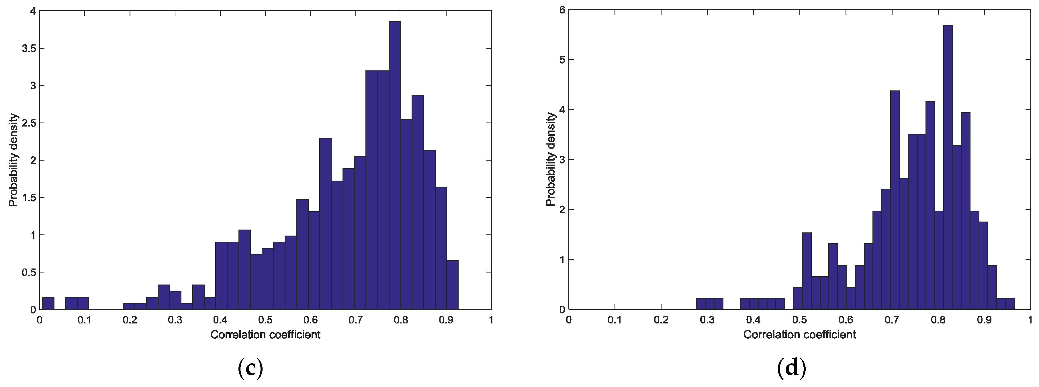
As one of results among cases, the correlation coefficient between wind farm Qiaodong II and wind turbine A015 was calculated. Consequently, its probability density distributions were obtained as seen in Figure 11, where the coefficient value “−1” means a negative correlation between the wind speed series of the wind farm and wind turbine A015 while the value “1” indicates a positive correlation between the two. Note that the overall blue area of each subplot is 1, which is the total probability of the correlation coefficient in the specific time interval. It is observed that the Pearson coefficients for short time scales (subplot (a) and (b)) range from −1 to 1 while those of long time scales (subplot (c) and (d)) range from 0 to 1.

As the time interval gets longer, the wind speed series in time of the wind farm and its wind turbines tend to get positively correlated, which indicates that variation and change of wind speed series tends to coincide in a long period (over 1 h). And as the time interval gets shorter, the Pearson coefficient values distribute between a negative correlation (−1) and a positive correlation (1), indicating a volatility and randomness in wind speed series of wind turbines located in the wind farm in a short period (under 1 h).

5.4. Correlation Characteristics of Wind Speed Among Wind Farms

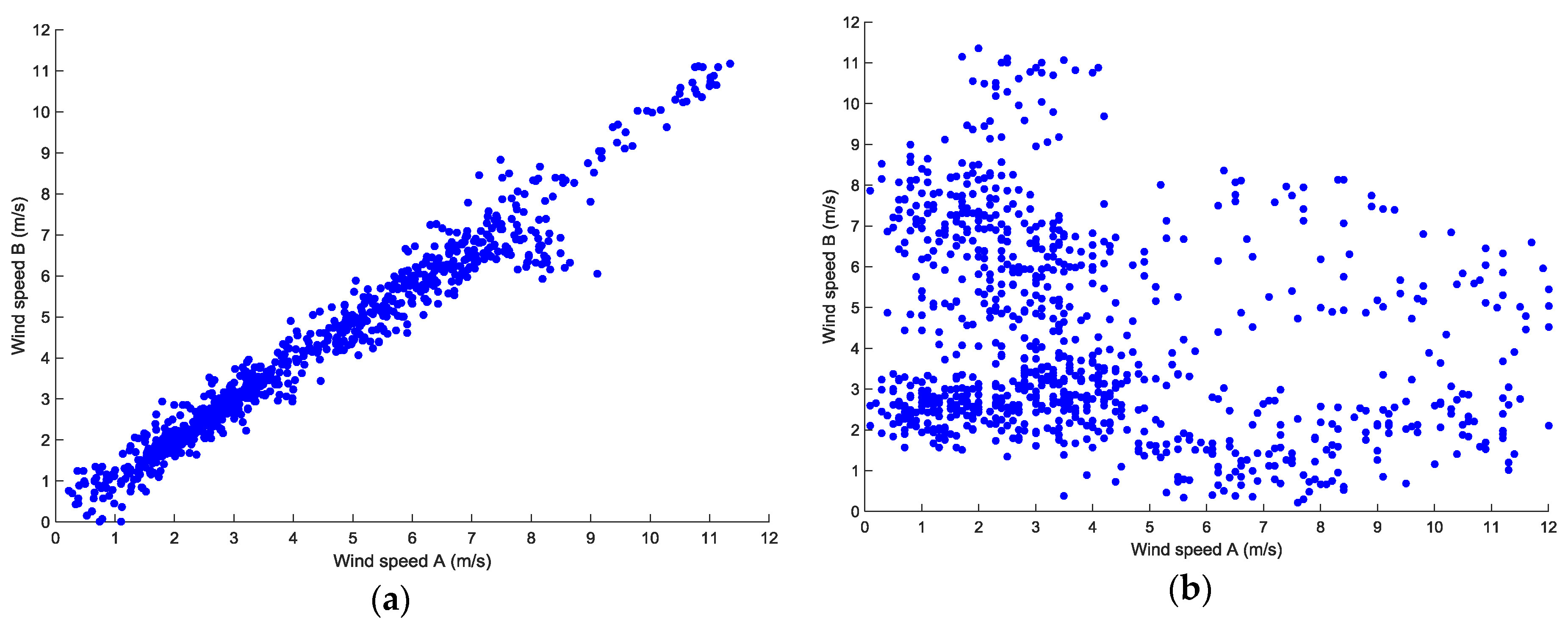
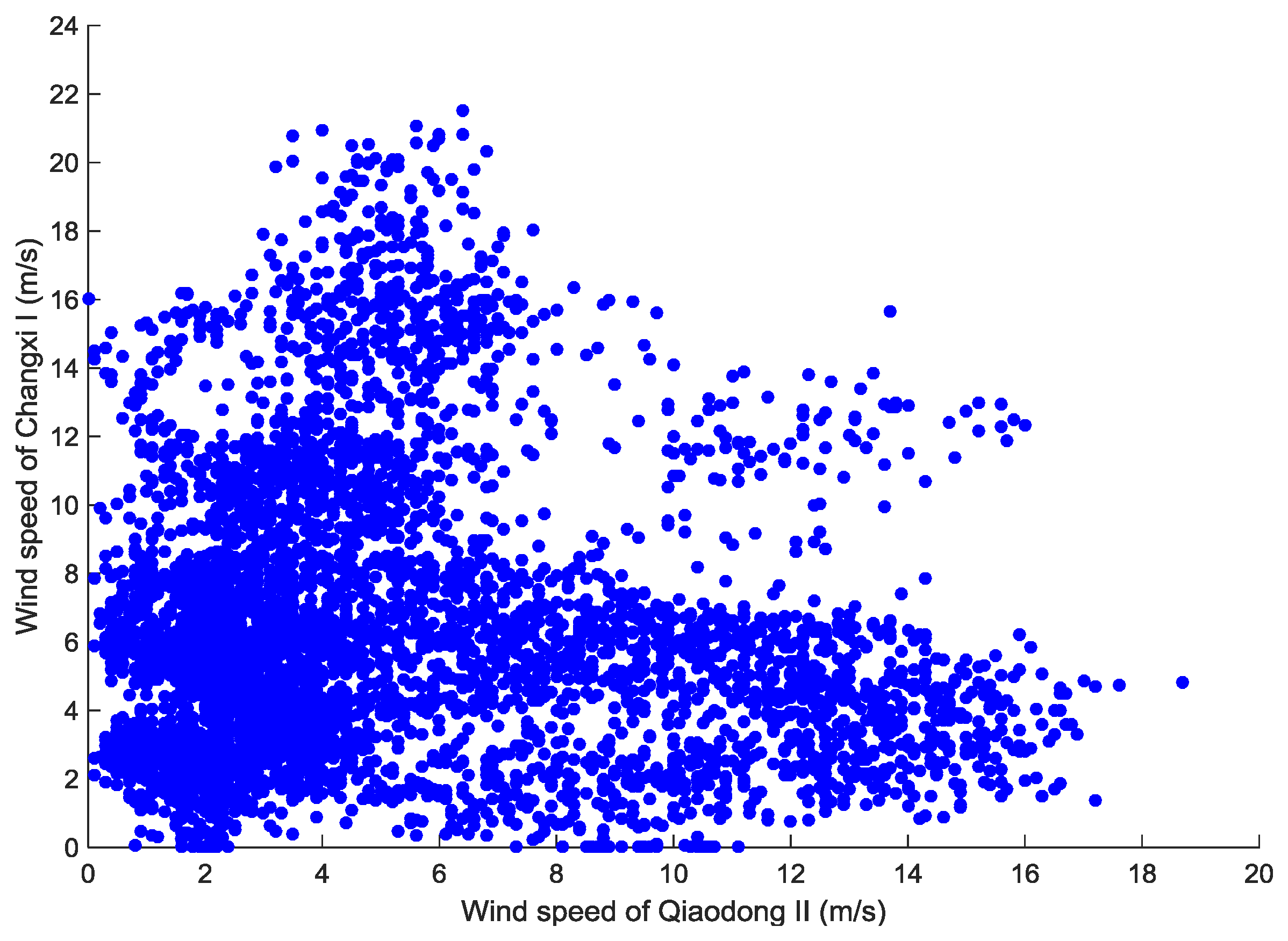
Wind speed series in the Qiaodong II and Changxi I wind farms were analyzed as an example to investigate the correlation characteristics of wind speed among wind farms. At a distance of 80 km, the wind speed of the two wind farms is not linearly correlated, which is shown in Figure 12 where wind speed points are scattered randomly and disorderly.

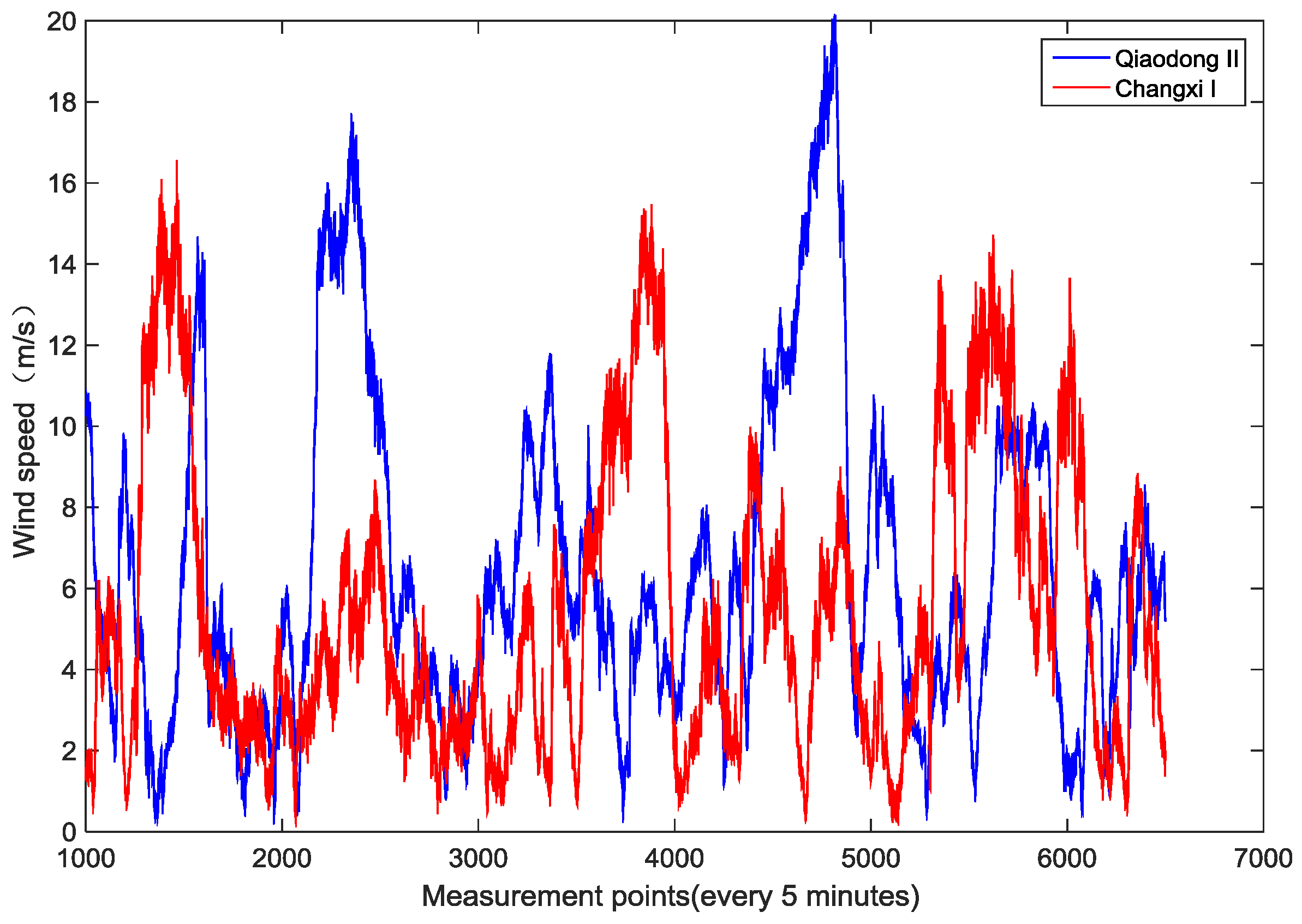
However, Figure 13 shows a dependent variation tendency of the wind speed series of two wind farms, and their nonlinear correlation deserves to be investigated using copula analysis.

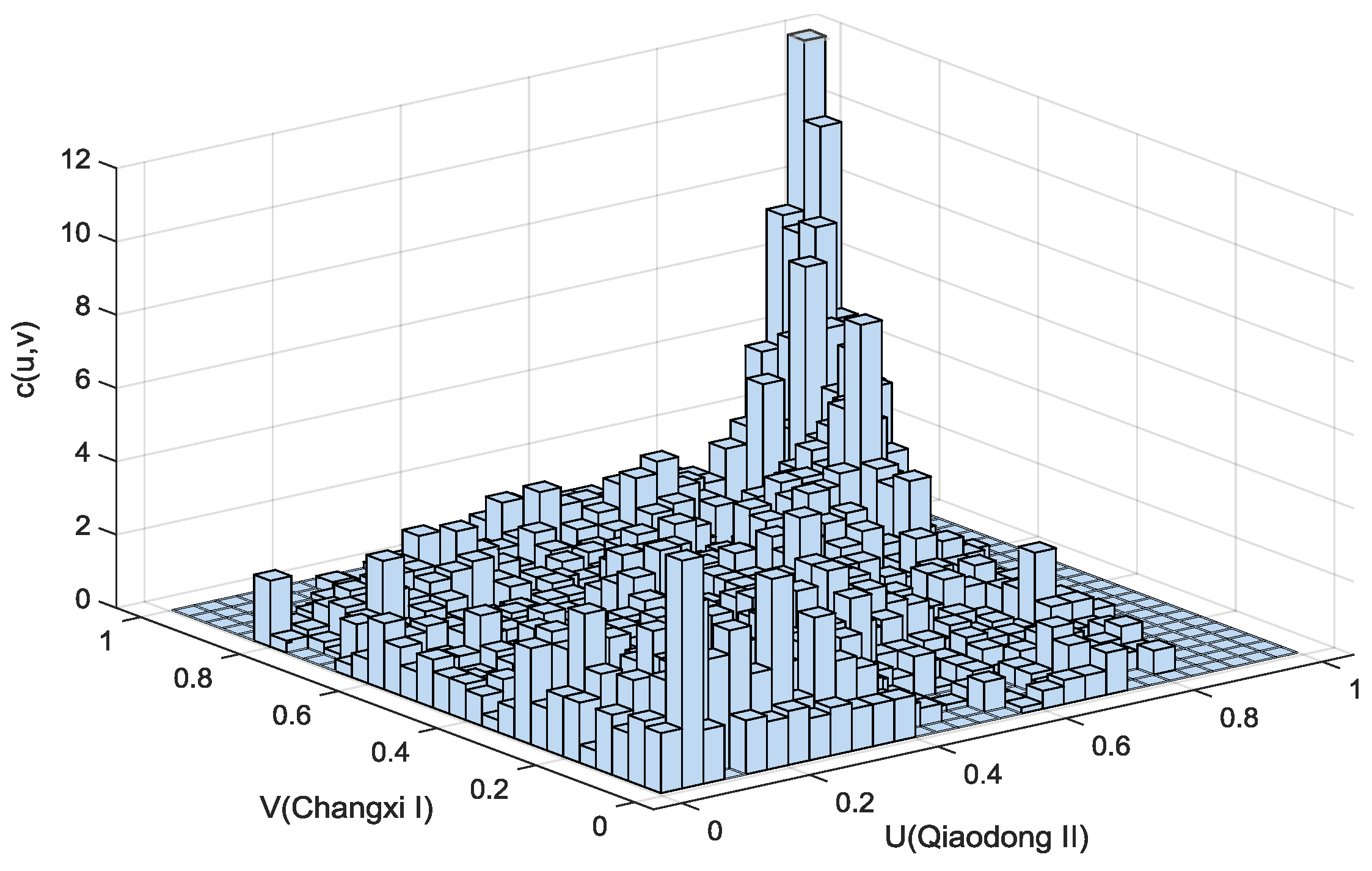
An asymmetric tail is shown in Figure 14 with a heavy upper tail and a light lower tail. After constructing the empirical Copula function, the Euclidean distances of common Copulas (Gauss, t, Gumbel, etc.) to the empirical Copula are calculated, respectively, to determine the best-fitted Copula function. The less the Euclidean distance of the specific Copula function to the empirical copula distribution is, the better the Copula function fits the actual joint distribution. As the results in

Table 4. Euclidean distance between Copulas and empirical Copula.

Type of Copula	Gauss_Copula	t_Copula	Gumbel_Copula	Frank_Copula	Clayton_Copula	Best-Fitted Copula
Euclidean Distance	1.3924	1.2160	0.0246	1.2127	4.8965	Gumbel

show, the Gumbel_Copula with its minimum Euclidean distance to the empirical Copula fits the best compared to other common copulas. Therefore, the Gumbel_Copula was chosen as the fitted-best copula to analyze the correlation of wind speed series between the Qiaodong II and Changxi I wind farms.

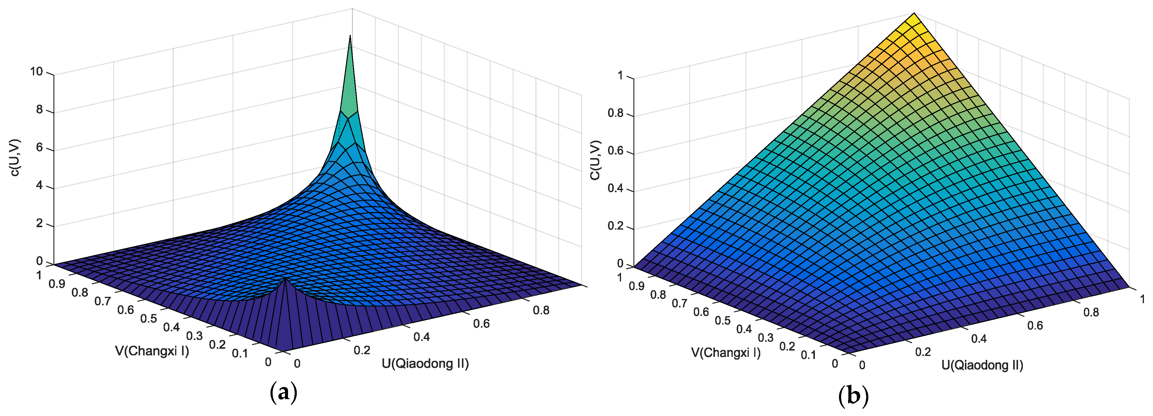
After estimating the parameters of the Gumbel function, the Gumbel_Copula probability density function was obtained as seen in Figure 15 where a “J” shaped feature is consistent with the bivariate frequency histogram in Figure 14. The Gumbel_Copula, which sensitively captures the upper tail variation of the correlation, indicates that the wind speed of the two wind farms has a strong dependence at the upper tail but an asymptotic independence at the lower tail in the joint probabilistic distribution.

Correlation coefficients are calculated to test the nonlinear correlation of wind speeds between the Qiaodong II and Changxi I wind farms. As the results listed in

Table 5. Results of correlation coefficients of wind speeds between two wind farms.

Copula Coefficients	Spearman	λup	λlo
Values	0.5952	0.8952	0

show, the Spearman rank coefficient is 0.5952, indicating that when the wind speed of Qiaodong II is increasing, the difference between the probability of increase in wind speed of Changxi I and the probability of decrease in wind speed of Changxi I is 0.5952. This illustrates that there is a moderate correlation of wind speed between the Qiaodong II and Changxi I wind farms.

The upper and lower tail coefficients λ^up and λ^lo are calculated when the threshold value is 0.95 and 0.05, respectively. It means that when the wind speed of Qiaodong II is over 20.3 m/s corresponding to “0.95” of its wind speed cumulative probability, the probability of the wind speed in Changxi I over 22.6 m/s corresponding to “0.95” of its cumulative probability is 0.8952. The heavy upper tail shows a strong wind speed correlation between the two wind farms in the high wind speed region. In low wind speed region which is under 3 m/s corresponding to “0.05” of either wind speed cumulative probability, the wind speeds of two farms tend to become independent.

The dependence structure of wind speed between Qiaodong II and Changxi I and their tail correlation are described in an intuitive way in the Gumbel_Copula function. It could provide detailed correlation information for a wind speed forecasting model, which can be transformed according to wind power curves to improve the wind power prediction accuracy.

6. Conclusions

The correlation characteristics of wind speed in different geographical hierarchies meaning among wind turbines, among a wind farm and its wind turbines, and among wind farms are of significance to the planning and operation of wind power bases as well as power systems. A new approach for correlation characteristics analysis was proposed in this paper. Both linear and nonlinear correlation coefficients are introduced to accommodate different wind speed correlation relationships. Analysis procedures in different geographical hierarchies were presented. Extensive case studies on the data from the Jiuquan Wind Power Base validated the proposed approach, and indicated that:

• As the distance of every two wind turbines in the same wind farm increases, there is a negative linear relationship in the correlation of instantaneous wind speed. This knowledge provides recommendations to enlarge the balancing areas and to construct transmission paths in diverse locations.
• The variation and change of wind speed series in time tends to coincide with in a long period (over 1 h) while the wind speed series of wind turbines are random and versatile in a short period (under 1 h).
• The dependence structure among wind farms with their tail correlations should be considered in wind speed forecasting, which provides a detailed understanding in general correlation characteristics of wind speed among wind farms to improve the accuracy of the wind speed forecasting model.

The conclusions above will be used for wind unit and farm siting and planning. The proposed study can provide detailed correlation information for a forecasting model of wind speed which can be transformed into wind power to improve the accuracy of wind power prediction and probabilistic power flow calculations. They are certainly of high interest in probability production simulation, which contributes to power system planning and risk assessment.

References

1. Graabak, I.; Korpas, M. Variability characteristics of European wind and solar power resources-a review. Energies 2016, 9, 449. [Google Scholar] [CrossRef]
2. Hong, Y.Y.; Yu, T.H.; Liu, C.Y. Hour-ahead wind speed and power forecasting using empirical mode decomposition. Energies 2013, 6, 6137–6152. [Google Scholar] [CrossRef]
3. Sun, W.; Liu, M.; Liang, Y. Wind speed forecasting based on FEEMD and LSSVM optimized by the Bat algorithm. Energies 2015, 8, 6585–6607. [Google Scholar] [CrossRef]
4. Morales, J.M.; Baringo, L.; Conejo, A.J.; Minguez, R. Probabilistic power flow with correlated wind sources. IET Gener. Trans. Distrib. 2010, 4, 641–651. [Google Scholar] [CrossRef]
5. Gao, Y.; Billinton, R. Adequacy assessment of generating systems containing wind power considering wind speed correlation. IET Renew. Power Gen. 2009, 3, 217–226. [Google Scholar] [CrossRef]
6. Qin, Z.; Li, W.; Xiong, X. Generation system reliability evaluation incorporating correlations of wind speeds with different distributions. IEEE Trans. Power Syst. 2013, 28, 551–558. [Google Scholar] [CrossRef]
7. Li, P.; Guan, X.; Wu, J.; Zhou, X. Modeling dynamic spatial correlations of geographically distributed wind farms and constructing ellipsoidal uncertainty sets for optimization–based generation scheduling. IEEE Trans. Sustain. Energy 2015, 6, 1594–1605. [Google Scholar] [CrossRef]
8. Valle, F.; Lobry, J.; Deblecker, O. Impact of the wind geographical correlation level for reliability studies. IEEE Trans. Power Syst. 2007, 22, 2232–2239. [Google Scholar] [CrossRef]
9. Xie, M.; Xiong, J.; Ke, S.; Liu, M. Two-stage compensation algorithm for dynamic economic dispatching considering Copula correlation multi-wind farms generation. IEEE Trans. Sustain. Energy 2016. [Google Scholar] [CrossRef]
10. Holttinen, H.; Hirvonen, R. Power System Requirements for Wind Power; John Wiley & Sons, Ltd.: New York, NY, USA, 2005; pp. 143–167. [Google Scholar]
11. Decarolis, J.F.; Keith, D.W. The economics of large-scale wind power in a carbon constrained world. Energy Policy 2006, 34, 395–410. [Google Scholar] [CrossRef]
12. Olauson, J.; Bladh, J.; Lonnberg, J.; Bergkvist, M. A new approach to obtain synthetic wind power forecasts for integration studies. Energies 2016, 9, 800. [Google Scholar] [CrossRef]
13. Wu, Q.; Peng, C. Wind power generation forecasting using least squares support vector machine combined with ensemble empirical mode decomposition, principal component analysis and a bat algorithm. Energies 2016, 9, 261. [Google Scholar] [CrossRef]
14. Feijoo, A.; Villanueva, D.; Pazos, J.L.; Sobolewski, R. Simulation of correlated wind speeds: A review. Renew. Sustain. Energy Rev. 2011, 15, 2826–2832. [Google Scholar] [CrossRef]
15. Xie, K.; Miao, S.; Ma, Y. A two-stage wind speed model for multiple wind farms considering autocorrelations and cross-correlations. In Proceedings of the International Conference on Probabilistic Methods Applied to Power Systems, Beijing, China, 16–20 October 2016.
16. Myers, J.L.; Well, A.D. Research Design and Statistical Analysis, 2nd ed.; Lawrence Erlbaum: Mahawh, NJ, USA, 2003; p. 508. [Google Scholar]
17. Louie, H. Evaluating Archimedean Copula models of wind speed for wind power modeling. In Proceedings of the IEEE PES Power Africa Conference and Exhibition, Johannesburg, South Africa, 9–13 July 2012.
18. Li, Y.; Xie, K.; Hu, B. Copula-ARMA model for multivariate wind speed and its applications in reliability assessment of generating systems. J. Electr. Eng. Technol. 2013, 8, 421–427. [Google Scholar] [CrossRef]
19. Lee, D.S.; Chang, C.S.; Chang, H.N. Analyses of the clustering coefficient and the Pearson degree correlation coefficient of Chung’s duplication model. IEEE Trans. Netw. Sci. Eng. 2016, 3, 117–131. [Google Scholar] [CrossRef]
20. Nelsen, R.B. An Introduction to Copulas, 2nd ed.; Springer: Berlin, Germany, 2006. [Google Scholar]
21. Shirley, C.G.; Daasch, W.R. Copula models of correlation: A DRAM case study. IEEE Trans. Comput. 2014, 63, 2389–2401. [Google Scholar] [CrossRef]
22. Xu, Q.; Chen, L.; Zeng, P.; Xu, X. Correlation modeling among multi-wind farms based on Copula-ARMA wind speed model. In Proceedings of the China International Conference on Electricity Distribution, Shenzhen, China, 23–26 September 2014.
23. Matteis, R.D. Fitting Copulas to Data. Ph.D Thesis, University of Zuricch, Zuricch, Switzerland, June 2001. [Google Scholar]
Figure 1. Sectionalized wind speed points in selecting process.
Energies 10 00237 g001
Figure 2. Flow chart of establishing the joint probability table of sectionalized wind speed of two wind turbines A1 and A2.
Energies 10 00237 g002
Figure 3. Scatter diagrams of paired wind speed values: (a) linear correlation of wind speed A and B; (b) nonlinear correlation or no-correlation of wind speed A and B.
Energies 10 00237 g003
Figure 4. Flow chart of correlation characteristic analysis in different hierarchies.
Energies 10 00237 g004
Figure 5. Wind speeds series in time of wind turbine A and B in a certain period: (a) before shifting the time difference; (b) after shifting the time difference.
Energies 10 00237 g005
Figure 6. Gansu wind areas and geographical altitudes of the Jiuquan wind power base.
Energies 10 00237 g006
Figure 7. Joint scatter diagram of wind speeds of wind turbines A001 and A134.
Energies 10 00237 g007
Figure 8. Wind speed series in time of wind turbines A001 and A134 in a certain period in the Qiaodong II wind farm.
Energies 10 00237 g008
Figure 9. Linear correlation coefficients with different shifted time intervals
Energies 10 00237 g009
Figure 10. Correlation coefficients in different geographical distances between any two wind turbines in the Qiaodong II wind farm.
Energies 10 00237 g010
Figure 11. Probability density distribution of correlation coefficients of wind speed between wind farm QiaodongII and wind turbine A015 in different time scales: (a) 0.5 h; (b) 1 h; (c) 6 h; (d) 12 h.
Energies 10 00237 g011aEnergies 10 00237 g011b
Figure 12. Scatter diagram of wind speeds of the Qiaodong II and Changxi I wind farms.
Energies 10 00237 g012
Figure 13. Wind speeds in time series of the Qiaodong II and Changxi I wind farms in a certain period.
Energies 10 00237 g013
Figure 14. Bivariate frequency histogram based on wind speeds of Qiaodong II and Changxi I.
Energies 10 00237 g014
Figure 15. Gumbel-Copula function based on wind speeds of Qiaodong II and Changxi I: (a) Gumbel-Copula probability density function; (b) Gumbel-Copula cumulative function.
Energies 10 00237 g015