An N-k Analytic Method of Composite Generation and Transmission with Interval Load

Abstract

N-k contingency estimation plays a very important role in the operation and expansion planning of power systems, the method of which is traditionally based on heuristic screening. This paper stringently analyzes the best and worst states of power systems given the uncertainties of N-k contingency and interval load. For the sake of simplification and tractable computation, an approximate direct current (DC) power flow model was used. Rigorous optimization models were established for identifying the worst and best scenarios considering the contingencies of generators and transmission lines together with their uncertain loads. It is very useful to identify the worst N-k contingencies with interval loads. If the worst existing scenario meets security standards, all scenarios must satisfy it. The mathematical model established for finding the worst N-k contingency with interval load is a bi-level optimization model. In this paper, strong duality theory and mathematical linearization were applied to the solution of bi-level optimization. The computational results of standard cases validate the effectiveness of the proposed method and illustrate that generator contingency has more impact on minimum load shedding than transmission line contingency.

1. Introduction

1.1. Motivation

Research on the security of power systems generally focuses on stability security based on differential equations and adequate security based on algebraic equations [1]. The study of adequate security is usually associated with static conditions that do not include dynamics and transient processes. Research on the adequacy of power systems under static conditions can be divided into two categories: probability analysis and the deterministic analysis of N-k contingency. This paper studies the deterministic analysis of power systems under the loss of k components for expansion planning.

N-1 and N-2 security criteria are applied to power industries all over the world, but the number of components out in cascading contingencies is usually more than two [2]. Severe contingencies are mainly caused by N-k cascading contingencies [3]; thus the analysis of N-k contingency is very valuable to operations and expansion planning. In this paper, the authors identify the best and worst N-k contingencies with uncertain loads from a stringent mathematical view. The problems examined are as follows:

(1)

Under certain load demands, which k transmission lines out produce the best N-k contingency, and which k transmission lines out produce the worst N-k contingency?

(2)

Under certain load demands, which k components that include transmission lines and generators out produce the best N-k contingency, and which k components out produce the worst N-k contingency?

(3)

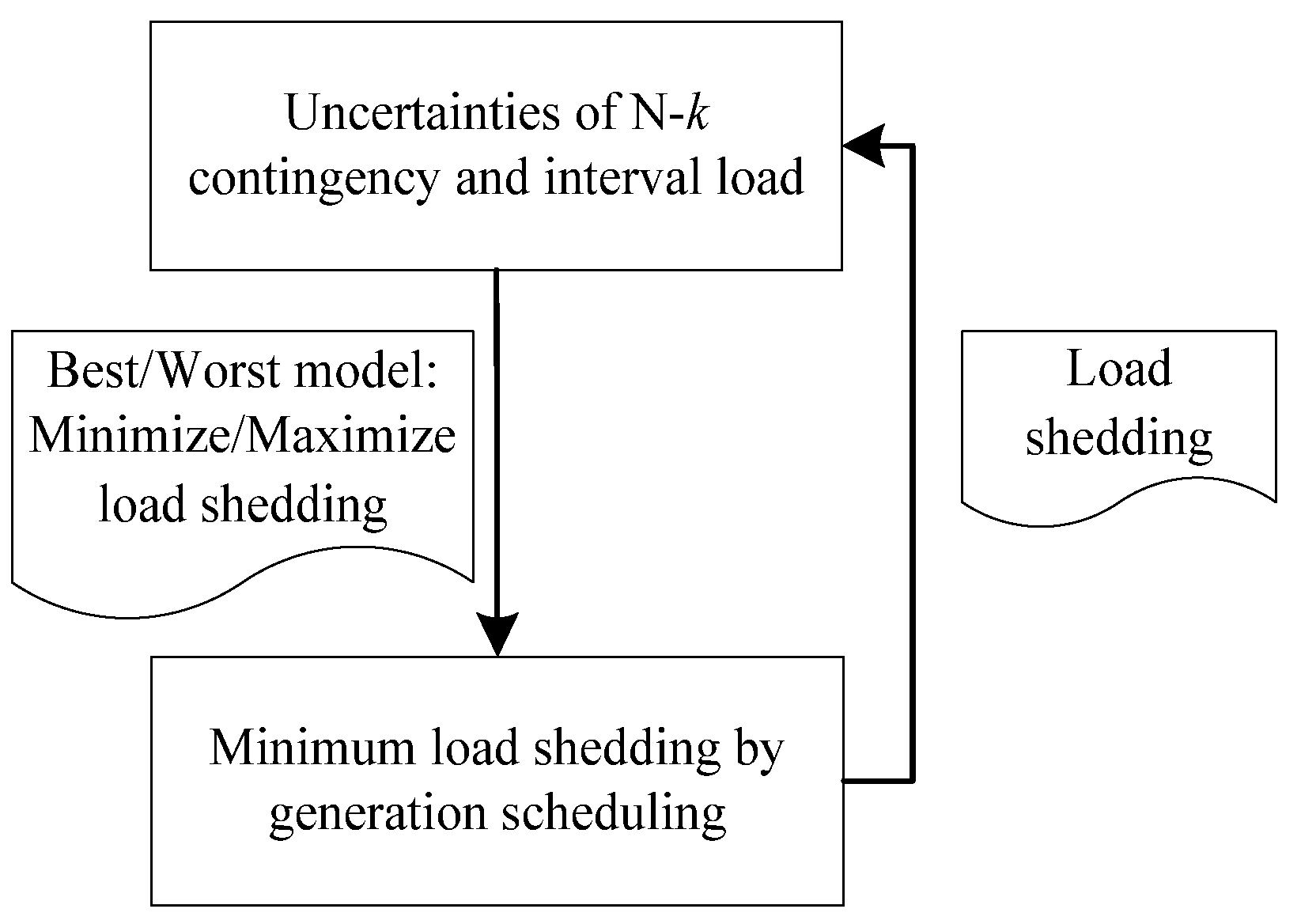
Under uncertain load demands, which k components out and which load blocks produce the best system state, and which k components out and load blocks produce the worst-case system state (WSS). The WSS refers to the worst-case scenario under uncertain conditions of N-k contingency and load demand.

In the real-world power industry, establishing the best-case scenario is pointless, because judgements of power system security are not based on best-case scenarios, which usually meet security standards. Power system operators or planners are concerned about worst-case scenarios under uncertain N-k contingencies and with varied loads, conditions that are weaker than all other power system scenarios given uncertainties of N-k contingency and load demand. If the worst scenario can meet the security criteria of its power system, all N-k contingencies with varied loads must also satisfy security criteria. Our main goal is therefore to identify the worst N-k contingency with varied load.

1.2. Literature Review and Contributions

Previous works mostly focus on N-1 and N-2 analysis, but there is some literature about the N-k contingency. N-k analysis of system operation is associated with cascading outages [4,5,6]. In power system expansion planning, minimum load shedding (MLS) is applied to the security analysis [7,8,9], and by applying MLS, the cascading outages associated with N-k can be considered [2]. The key to N-k analysis is how to choose the k components. If we know the special k components, N-k analysis is essentially an operation problem with k components out. However, it is very difficult to select the relevant k components of the worst scenario from all system components. Screening all contingencies is one method, but it is very clumsy, especially under large k numbers. With k increasing, the combined number of N-k contingencies is enormous. Thus contingency screening requires special skills or techniques, especially with regard to dynamic security research [10,11]. Because of the enormous amount of complete contingency screening, N-k contingency is usually studied by the heuristic method. Reference [12] proposes the linear sensitivities for fast N-2 contingency screening. Reference [5] uses quantum-inspired multi-objective evolutionary algorithms for N-k cascading contingency screening. Both use the heuristic method and do not consider uncertain loads. In real-world power systems, the load demand is changeable or the predicted load may be in error. Therefore, heuristic methods cannot usually cover all contingencies.

There is some literature about N-k contingencies or uncertain loads from a stringent mathematical view. Reference [8] studies the security analysis of transmission expansion planning (TEP) with interval loads, but does not consider the outages of transmission lines and generators. Reference [13] researches the worst contingencies of transmission line loss by an optimization method, which does not account for the contingencies of generators and uncertain loads. In reference [14], the worst contingencies can be found in the credit contingency set, and the uncertainties, and preventive and corrective actions of generation units, are considered with alternative current power flow. Reference [15] studies the stochastic and robust unit commitment with uncertainty. Reference [16] studies the bi-level optimization of the terrorist threat problem, but only considers transmission lines.

Within this context, the main contributions of this paper are as follows:

(1)

From a stringently mathematical view, we establish two models for identifying the best and worst scenarios given the uncertainties of N-k contingency and load demand. These models are based on a minimum load shedding problem with linearized DC power flow. All N-k contingencies with generators and lines and interval loads were considered in this paper. The model used for identifying the best scenario is single mixed integer linear programming, but identifying the worst scenario is a bi-level optimization problem. Compared with the model for the best scenario, therefore, the model for the worst scenario is complex and applicable in real-world power systems. Therefore, we mainly focus on the model for identifying the worst scenario.

(2)

Applying strong duality theory and mathematical linearization methods, we transformed the bi-level optimization of identifying the worst scenario into a mixed integer linear program (MILP). The MILP can be mathematically solved by mature optimization software. The mathematical method of linear bi-level optimization has already been matured [15,17]; hence, the paper mainly uses strong duality and linearization method for the bi-level model solution.

(3)

Detailed analyses of N-k contingencies with IEEE-RTS-24 and IEEE-118 bus systems were performed. These numerical studies demonstrate the effectiveness of the MILP method for identifying the worst-case scenario and illustrate the impact of generator contingencies on N-k analysis.

1.3. Paper Organization

The remaining sections of the paper are organized as follows. Section 2 formulates the best and worst system states of N-k contingency. Section 3 provides the model solution as a strong duality theorem and linearized method. The numerical cases with IEEE-RTS-24 and IEEE-118 bus systems are explained and discussed in Section 4. Conclusions and areas for future research are given in Section 5.

2. Problem Formulations

2.1. Model Assumptions

N-k contingencies cover a broad range of searches, so it is very difficult to find the worst or best contingency. In order to simplify the analysis of N-k contingency and make the problem tractable, some assumptions are summarized below:

(1)

Our models only consider active power flow with a linearized DC power flow model, which in fact are widely applied to the risk assessment of power systems, static contingency analysis, long-term expansion planning [18] and unit commitment with transmission constraints [19].

(2)

Details of up, down and ramp constraints of generators are neglected. We assume generation units can be re-dispatched quickly under post contingency.

(3)

Only load shedding quantifies the quality of the state of the N-k contingency. The indicator for ranking all contingencies is only load shedding, which is useful to power system expansion planning [8].

(4)

Interval load demand describes the uncertain loads [8].

The first and second items above aim to approximate the operation of power systems. Neglecting reactive power and detail unit commitments has some impact on the analysis of N-k contingencies with interval load, but linearized DC power flow and simple generation scheduling are useful to long-term expansion planning and rough operation planning. Because only load shedding is used to rank all contingencies, the optimization model for identifying the best or worst scenario used the load shedding value as the objective function. When the contingency elements and load demand are known, the operation problem is minimum load shedding, which is widely applied to the security judgement of expansion planning [8,9,20]. Thus these models for identifying the worst- or best-case scenarios under N-k contingency and interval loads can be comprehended as a two-stage robust optimization problem [15]. Figure 1 is a diagram of the model. As Figure 1 shows, uncertainties of N-k contingencies and interval loads will minimize load shedding for the best-case scenario, so the model for identifying the best-case scenario is a mathematical minimum problem, called the best system state model. Because uncertainties of N-k contingencies and interval loads will maximize load shedding for worst-case scenarios, the model for identifying the worst-case scenario is a max-min problem, called the worst system state model.

2.2. The Best-Case System State Model of N-k Contingency

The best-case state model minimizes load shedding in Equation (1), subject to N-k contingency and interval load constraints, as shown in Equations (2)–(4). Operation constraints based on linearized DC power flow models are shown in Equations (5)–(9). They are formulated as follows:

$$\underset{\mathsf{\Xi }}{\min }{\displaystyle \sum _i{r}_i}$$

(1)

$$s.t.{\displaystyle \sum _{\left(ij,k\right)\in \mathsf{\Omega }}\left(1-e_{ij,k}\right)}+{\displaystyle \sum _{\left(i,k\right)\in G}\left(1-e_{i,k}\right)}\ge k$$

(2)

$${\underset{\_}{d}}_i\le d_i\le {\overline{d}}_i\forall i\in N$$

(3)

$$e_{ij,k},e_{i,k}\in \left\{0,1\right\}\forall \left(ij,k\right)\in \mathsf{\Omega },\left(i,k\right)\in G$$

(4)

$${\displaystyle \sum _{(i,k)\in G_i}{g}_{i,k}}-{\displaystyle \sum _{\left(ij,k\right)=l\in \mathsf{\Omega }}{A}_{il}}{f}_{ij,k}+r_i=d_i\forall i\in N$$

(5)

$$f_{ij,k}=e_{ij,k}{b}_{ij,k}\left({\theta }_i-{\theta }_j\right)\forall \left(ij,k\right)\in \mathsf{\Omega }$$

(6)

$$-{\overline{f}}_{ij,k}\le f_{ij,k}\le {\overline{f}}_{ij,k}\forall \left(ij,k\right)\in \mathsf{\Omega }$$

(7)

$$0\le g_{i,k}\le e_{i,k}{\overline{g}}_{i,k}\forall \left(i,k\right)\in G$$

(8)

$$0\le r_i\le d_i\forall i\in N$$

(9)

In the model above, the decision variables are as follows: which transmission lines ($e_{ij,k}$) and generation units ($e_{i,k}$) will be lost, the load demand of bus$i$ ($d_i$), operation variables for the power angle (${\theta }_i$), line real power ($f_{ij,k}$), generation power output ($g_{i,k}$), and load shedding ($r_i$). The decision variables set is $\mathsf{\Xi }=\left\{e_{ij,k},e_{i,k},d_i,{\theta }_i,f_{ij,k},g_{i,k},r_i\right\}$. Variables $e_{ij,k}$ and $e_{i,k}$ are binary: their values are 0 when contingencies occur, 1 otherwise. The objective function minimizes total load shedding as Equation (1). Equations (2) and (4) denote that the number of contingency elements is not smaller than the value of k. Equation (3) expresses interval load. Equation (5) denotes real power balance at each node or bus, Equation (6) expresses linearized DC power flow equations of all lines, Equation (7) describes the limits of line capacity, Equation (8) calculates the limits of generators output, and Equation (9) calculates the limit of load shedding. If the loss of generators is not considered, the state variable of generation units (e_i,k) is omitted. If the load demand is known, Equation (3) is omitted. The best-state model can provide the information that load shedding must occur at certain demand scenarios when k is more than a certain value. If the optimal value of the best state model is more than zero at certain k₀, load shedding must occur at certain demand scenarios over all N-k contingencies, the k values of which are equal to or more than k₀.

2.3. Worst-Case System State Model of N-k Contingency

The model of WSS is a bi-level optimization problem. Its decision variables can be divided into two categories: ${\mathsf{\Xi }}_1=\left\{e_{ij,k},e_{i,k},d_i\right\}$ from upper level model and ${\mathsf{\Xi }}_2=\left\{{\theta }_i,f_{ij,k},g_{i,k},r_i\right\}$ from lower level model. The decision variables of upper level optimization identify the contingencies of which transmission lines and generators and what load demand is made at each load bus under uncertain loads. When the operator knows the k contingency and load scenario, the lower level optimization model minimizes total load shedding by generation dispatch. The uncertainties of N-k contingency and load maximizes the total load shedding from the lower level problem. These formulations of the WSS model are as follows:

$$\underset{{\mathsf{\Xi }}_1}{\max }{\displaystyle \sum _i{r}_i^{*}}$$

(10)

$$s.t.{\displaystyle \sum _{\left(ij,k\right)\in \mathsf{\Omega }}\left(1-e_{ij,k}\right)}+{\displaystyle \sum _{\left(i,k\right)\in G}\left(1-e_{i,k}\right)}\le k$$

(11)

$${\underset{\_}{d}}_i\le d_i\le {\overline{d}}_i\forall i\in N$$

(12)

$$e_{ij,k},e_{i,k}\in \left\{0,1\right\}\forall \left(ij,k\right)\in \mathsf{\Omega },\left(i,k\right)\in G$$

(13)

$$r_i^{*}\in \arg \{\underset{{\mathsf{\Xi }}_2}{\min }{\displaystyle \sum _i{r}_i}|$$

(14)

$$s.t.{\displaystyle \sum _{(i,k)\in G_i}{g}_{i,k}}-{\displaystyle \sum _{\left(ij,k\right)=l\in \mathsf{\Omega }}{A}_{il}}{f}_{ij,k}+r_i={\widehat{d}}_i\forall i\in N$$

(15)

$$f_{ij,k}={\widehat{e}}_{ij,k}{b}_{ij,k}\left({\theta }_i-{\theta }_j\right)\forall \left(ij,k\right)\in \mathsf{\Omega }$$

(16)

$$-{\overline{f}}_{ij,k}\le f_{ij,k}\le {\overline{f}}_{ij,k}\forall \left(ij,k\right)\in \mathsf{\Omega }$$

(17)

$$0\le g_{i,k}\le {\widehat{e}}_{i,k}{\overline{g}}_{i,k}\forall \left(i,k\right)\in G$$

(18)

$$0\le r_i\le {\widehat{d}}_i\forall i\in N$$

(19)

where superscript $*$ denotes the variables from lower level optimization model and the minimum load shedding ($r_i^{*}$); superscript ˆ indicates the variables from the upper level optimization model, the contingency state of lines and units (${\widehat{e}}_{ij,k}$ and ${\widehat{e}}_{i,k}$), and load demand (${\widehat{d}}_i$). Note that the upper-level model maximizes minimum load shedding from lower-level optimization given the N-k contingency of transmission lines and generators and uncertain load. Equation (11) is different from Equation (2). The number of contingencies in the model of WSS is smaller than or equal to k. Equations (14)–(19) express the minimum load shedding problem that is widely applied to TEP [8,9]. When the contingencies of generators and uncertain loads are not integrated, the corresponding Equations (11)–(13) and (18) are corrected or omitted. In order to conveniently describe the solution of the WSS model, the bi-level model with compact matrix is presented below:

$$\underset{x_1,x_2}{\max }{c_1}^T{y}^{*}+{c_3}^{T}x$$

(20)

$$s.t.A_{1}x+B_1{y}^{*}\ge b_1$$

(21)

$$x_1\in \left\{0,1\right\}$$

(22)

$$y^{*}\in \arg \{\underset{y}{\min }{c_2}^{T}y+{c_4}^T\widehat{x}|$$

(23)

$$s.t.A_2(\widehat{x})+B_2(\widehat{x})y=b_2:\lambda$$

(24)

$$A_3(\widehat{x})+B_3(\widehat{x})y\ge b_3:\mathsf{\mu }$$

(25)

Variables and parameters are expressed as vectors and matrices. Equations (20)–(25) are a class bi-level linear programming problem when $B_2(\widehat{x})$ and $B_3(\widehat{x})$ are constant matrices. In the WSS model, $x_1$ is the state variable of transmission lines and generation units, $x_2$ is the load variable and other variable corresponding to the decision variables of the lower model of the WSS model, $c_1$ equals $c_2$, and $c_3$, $c_4$ and $B_1$ are 0. $A_2(\widehat{x})$ is associated with the uncertain load of the upper model of the WSS model, $A_3(\widehat{x})$ expresses the generation units of the upper model of the WSS model, $B_2(\widehat{x})$ refers to the transmission lines of the upper model of the WSS model, $B_3(\widehat{x})$ is a constant matrix, $B_3(x)=B_3$, and $\lambda$ and $\mathsf{\mu }$ are respectively the dual variables of Equations (24) and (25).

3. Model Solution

3.1. Single-Level Formulation

The model of the best-case state of N-k contingency can be easily solved by existing programming software, so the key to N-k contingency analysis is the solution of the WSS model. The bi-level linear optimization model can be transformed into a single-level optimization model because the lower model is convex under the fixed value of decision variables of the upper level problem. There are two methods that can achieve the transformation and are widely applied to research on power systems under power deregulation [21,22,23], respectively:

(1)

Under Karush–Kuhn–Tucker (KKT) conditions, the lower-level model can be substituted with its primal constraints, its dual constraints and its complementarity constraints.

(2)

Using primal and dual formulation (PD), the strong duality theorem (SDT) equality replaces its complementarity constraints.

Although both methods are equally valid, the linearization of the complementarity constraints associated with every inequality constraint of the lower-level model involves large numbers and auxiliary binary variables. In Reference [22], using the PD method, the bi-level equilibrium optimization model of TEP is successfully transformed into a single-level optimization method. Thus, the PD method is also applied here. Considering the special WSS model, the bi-level model expressed in Equations (20)–(25) is transformed into a single-level model as follows:

$$\underset{x,y,\lambda ,\mathsf{\mu }}{\max }{c_1}^{T}y$$

(26)

$$s.t.A_{1}x\ge b_1,x_1\in \left\{0,1\right\}$$

(27)

$$A_2(x)+B_2(x)y=b_2$$

(28)

$$A_3(x)+B_{3}y\ge b_3$$

(29)

$$B_2{\left(x\right)}^T\lambda +{B_3}^T\mathsf{\mu }=c_2,\mathsf{\mu }\ge 0$$

(30)

$${c_2}^{T}y={\lambda }^T\left(b_2-A_2\left(x\right)\right)+{\mathsf{\mu }}^T\left(b_3-A_3\left(x\right)\right)$$

(31)

Equations (28)–(31) express the constraints under which the lower level model is equivalent according to the SDT, Equations (28) and (29) express the primal feasibility constraints of the lower level model, Equation (30) expresses the dual feasibility constraints, and Equation (31) is the SDT equality. Equations (26)–(31) is a mixed integer nonlinear programing because they incorporate the product of dual variables and, respectively, $B_2(x)$, $A_2\left(x\right)$ and $A_3\left(x\right)$, but they can be linearized by mathematic methods. When the contingencies of generators and uncertain loads cannot be considered, $A_2\left(x\right)$ and $A_3\left(x\right)$ are constant and the only nonlinear element is associated with $B_2(x)$.

3.2. Linearized Formulation

Equations (28), (30), and (31) can be linearized. Equation (28) corresponds to Equation (16) of the WSS model, and we linearize them by substituting Equations (16) and (17) as follows:

$$-\left(1-e_{ij,k}\right)M_{ij,k}\le f_{ij,k}-b_{ij,k}\left({\theta }_i-{\theta }_j\right)\le \left(1-e_{ij,k}\right)M_{ij,k}\forall \left(ij,k\right)\in \mathsf{\Omega }$$

(32)

$$-e_{ij,k}{\overline{f}}_{ij,k}\le f_{ij,k}\le e_{ij,k}{\overline{f}}_{ij,k}\forall \left(ij,k\right)\in \mathsf{\Omega }$$

(33)

where the big number $M_{ij,k}$ is the product of susceptance and maximum angle difference of the transmission line. If the big number is large enough, Equations (32) and (33) are equivalent to Equations (16) and (17). The maximum angle difference of lines is usually very small: reference [23] recommends using a value of 1.2 rad. The value used in this paper is 1.5 rad, which is large enough to per-unit power systems; thus, M_ij,k equal to 1.5 b_ij,k in this paper.

The dual variables of Equations (15)–(19) of the WSS model are respectively ${\lambda }_i^1$, ${\lambda }_{ij,k}^2$, ${\underset{\_}{\mu }}_{ij,k}^1$, ${\overline{\mu }}_{ij,k}^1$, ${\underset{\_}{\mu }}_{i,k}^2$, ${\overline{\mu }}_{i,k}^2$, ${\underset{\_}{\mu }}_i^3$, and ${\overline{\mu }}_i^3$ (note that superscript numbers 1, 2, and 3 denote types of dual variables, not square and cube). Using dual transformation, Equation (30) expresses the constraints on the dual lower optimization problems, Equations (14)–(19), as follows:

$${\displaystyle \sum _{\left(ij,k\right)=l\in \mathsf{\Omega }}{A}_{il}{b}_{ij,k}{\lambda }_{ij,k}^2{e}_{ij,k}}=0\forall i\in N$$

(34)

$$-{\lambda }_i^1-{\underset{\_}{\mu }}_{i,k}^2+{\overline{\mu }}_{i,k}^2=0\forall \left(i,k\right)\in G$$

(35)

$${\displaystyle \sum _i{A}_{il}{\lambda }_i^1}-{\lambda }_{ij,k}^2-{\underset{\_}{\mu }}_{ij,k}^1+{\overline{\mu }}_{ij,k}^1=0\forall \left(ij,k\right)=l\in \mathsf{\Omega }$$

(36)

$$1-{\lambda }_i^1-{\underset{\_}{\mu }}_i^3+{\overline{\mu }}_i^3=0\forall i\in N$$

(37)

$${\underset{\_}{\mu }}_{ij,k}^1,{\overline{\mu }}_{ij,k}^1,{\underset{\_}{\mu }}_{i,k}^2,{\overline{\mu }}_{i,k}^2,{\underset{\_}{\mu }}_i^3,{\overline{\mu }}_i^3\ge 0$$

(38)

The only non-linear element in formulations above is ${\lambda }_{ij,k}^2{e}_{ij,k}$ in Equation (34). The product of the continuous variable and the binary variable can be linearized using the big number M method [22]. The linearization method is theoretically accurate if the big number is large enough. We assume ${\lambda }_{ij,k}^2{e}_{ij,k}$ equals $a_{ij,k}^1$, and introduce the auxiliary variable $a_{ij,k}^2$ and the upper and lower bounds of ${\lambda }_{ij,k}^2$. Because the dual multiplier of MLS in per-unit of power system is not greater than 1, we can set the big number value at 100. Applying the big number M method, the linearized equations making up Equation (34) are as follows:

$${\displaystyle \sum _{\left(ij,k\right)=l\in \mathsf{\Omega }}{A}_{il}{b}_{ij,k}{a}_{ij,k}^1}=0\forall i\in N$$

(39)

$$a_{ij,k}^1={\lambda }_{ij,k}^2-a_{ij,k}^2\forall \left(ij,k\right)\in \mathsf{\Omega }$$

(40)

$$-100e_{ij,k}\le a_{ij,k}^1\le 100e_{ij,k}\forall \left(ij,k\right)\in \mathsf{\Omega }$$

(41)

$$-100\left(1-e_{ij,k}\right)\le a_{ij,k}^2\le 100\left(1-e_{ij,k}\right)\forall \left(ij,k\right)\in \mathsf{\Omega }$$

(42)

The linear Equations (39)–(42) replace the nonlinear Equation (34); they are equivalent because the big number M is large enough. According to strong dual theory, the objective function of MLS is equal to that of the dual problem, called the strong duality equality. Equation (31) expresses the constraints of the strong duality equality, which can be rewritten as:

$${\displaystyle \sum _i{r}_i}={\displaystyle \sum _{\left(i,k\right)\in G}\left(-{\overline{\mu }}_{i,k}^2{e}_{i,k}{\overline{g}}_{i,k}\right)}+{\displaystyle \sum _{i\in N}\left({\lambda }_i^1-{\overline{\mu }}_i^3\right)}{d}_i-{\displaystyle \sum _{\left(ij,k\right)\in \mathsf{\Omega }}\left({\underset{\_}{\mu }}_{ij,k}^1+{\overline{\mu }}_{ij,k}^1\right)}{\overline{f}}_{ij,k}$$

(43)

The value for ${\overline{\mu }}_{i,k}^2{e}_{i,k}$ of Equation (43) is also linearized by the big number M method above. We assume ${\overline{\mu }}_{i,k}^2{e}_{i,k}$ equals $a_{i,k}^3$ and introduce auxiliary variable $a_{i,k}^4$. The linearized formulations are as follows:

$$a_{i,k}^3={\overline{\mu }}_{i,k}^2-a_{i,k}^4\forall \left(i,k\right)\in G$$

(44)

$$-100e_{i,k}\le a_{i,k}^3\le 100e_{i,k}\forall \left(i,k\right)\in \mathsf{\Omega }$$

(45)

$$-100\left(1-e_{i,k}\right)\le a_{i,k}^4\le 100\left(1-e_{i,k}\right)\forall \left(i,k\right)\in G$$

(46)

The $\left({\lambda }_i^1-{\overline{\mu }}_i^3\right)d_i$ of Equation (43) can be linearized by the Fortuny–Amat linearized method. Reference [21] successfully linearized the product of generation power and the dual variable by the Fortuny–Amat method, which was applied to the linearization of $\left({\lambda }_i^1-{\overline{\mu }}_i^3\right)d_i$ in this paper. We discretize the interval load by trisection and assume ${\Delta }_i$ equals $\left({\overline{d}}_i-{\underset{\_}{d}}_i\right)/3$. The linearization formulations are as below:

$$d_i={\underset{\_}{d}}_i+{\Delta }_i{n}_{i1}^d+2{\Delta }_i{n}_{i2}^d\forall i\in N$$

(47)

$$(n_{i1}^d,n_{i2}^d)\in \left\{0,1\right\}$$

(48)

$$\left({\lambda }_i^1-{\overline{\mu }}_i^3\right)d_i=\left({\lambda }_i^1-{\overline{\mu }}_i^3\right){\underset{\_}{d}}_i+{\Delta }_i{a}_{i1}^d+2{\Delta }_i{a}_{i2}^d\forall i\in N$$

(49)

$$-100\left(1-n_{i1}^d\right)\le {\lambda }_i^1-{\overline{\mu }}_i^3-a_{i1}^d\le 100\left(1-n_{i1}^d\right)\forall i\in N$$

(50)

$$-100n_{i1}^d\le a_{i1}^d\le 100n_{i1}^d\forall i\in N$$

(51)

$$-100\left(1-n_{i2}^d\right)\le {\lambda }_i^1-{\overline{\mu }}_i^3-a_{i2}^d\le 100\left(1-n_{i2}^d\right)\forall i\in N$$

(52)

$$-100n_{i2}^d\le a_{i2}^d\le 100n_{i2}^d\forall i\in N$$

(53)

where the value of the load demand at every bus has four options: the upper bound, the lower bound, the first value in the interval, or the second value in the interval. For greater accuracy, more steps can be considered. In this paper, trisection is adequate for the computation of case studies. In order to accelerate the convergence of mixed integer linear programming, the lower bound of Equations (50)–(53) can be set at 0 because ${\lambda }_i^1$ is generally larger than ${\overline{\mu }}_i^3$. We compare the computational time. When the lower bound is 0, the convergence speed is quicker than that of −100, and their solutions are the same. Through the above transformation, the linearization of Equation (43) is:

$${\displaystyle \sum _i{r}_i}={\displaystyle \sum _{\left(i,k\right)\in G}\left(-a_{i,k}^3{\overline{g}}_{i,k}\right)}-{\displaystyle \sum _{\left(ij,k\right)\in \mathsf{\Omega }}\left({\underset{\_}{\mu }}_{ij,k}^1+{\overline{\mu }}_{ij,k}^1\right)}{\overline{f}}_{ij,k}+{\displaystyle \sum _{i\in N}\left[\left({\lambda }_i^1-{\overline{\mu }}_i^3\right){\underset{\_}{d}}_i+{\Delta }_i{a}_{i1}^d+2{\Delta }_i{a}_{i2}^d\right]}$$

(54)

By linearizing the WSS model, a single MILP can be expressed, the decision variables of which include the primal variables $\mathsf{\Xi }=\left\{e_{ij,k},e_{i,k},d_i,{\theta }_i,f_{ij,k},g_{i,k},r_i\right\}$, and dual variables and auxiliary variables as follows:

$${\mathsf{\Xi }}_3=\left\{{\lambda }_i^1,{\lambda }_{ij,k}^2,{\underset{\_}{\mu }}_{ij,k}^1,{\overline{\mu }}_{ij,k}^1,{\underset{\_}{\mu }}_{i,k}^2,{\overline{\mu }}_{i,k}^2,{\underset{\_}{\mu }}_i^3,{\overline{\mu }}_i^3\right\}$$

(55)

$${\mathsf{\Xi }}_4=\left\{a_{ij,k}^1,a_{ij,k}^2,a_{i,k}^3,a_{i,k}^4,n_{i1}^d,n_{i2}^d,a_{i1}^d,a_{i2}^d\right\}$$

(56)

The MILP of the WSS model comprises Equations (5), (8)–(13), (32), (33), (35)–(42), (44)–(48), and (50)–(54), which are also presented together in the appendix. The MILP can be solved by mature programming software, making the WSS model tractable for computation. Here, two linearization methods are used: the big number M and Fortuny–Amat methods. The big number M method is very accurate for linearization if the big number M is large enough. The Fortuny–Amat method is an approximate method, only used for the interval load. Reference [8] proves and demonstrates the accuracy of MLS for determining interval load. This method is reasonable applied to real-world power systems for determining interval loads.

4. Numerical Studies

The numerical studies are implemented with the IEEE-RTS-24 bus system [24] and the IEEE-118 bus system [25]. The IEEE-RTS-24 bus system comprises 33 transmission lines, 5 transformers, 32 generation units, and 17 load buses. Transformers are regarded as transmission lines, thus totaling 38 lines. Five units carrying 12 MW at Bus 15 are merged into one unit of 60 MW, so the total number of units is 28. The total capacity of units installed is 3405 MW. The peak load demand is 2850 MW. The upper bound of the load demand is the peak load, and the lower bound around 90% of peak load. Other details of lines, bus number, peak load and units refer to reference [24].

Four cases under the IEEE-RTS-24 bus system were studied. Case 1 is the best- and worst-case system state under N-k contingency of lines with peak load; case 2 is the worst-case system state of N-k contingency of lines with interval loads; case 3 is the worst-case system state of N-k contingency of lines and generators with peak loads; and case 4 is the worst-case system state of N-k contingency of lines and generators with interval loads. The worst-case state is more applicable to our purposes than the best-case state and it is also easy to identify the best state, so only case 1 tested the best state to illustrate the applicability of the method. All cases tested worst-case states of N-k contingency. To evaluate the scalability of the analytical method of the worst state calculation, the worst load shedding of N-k contingency of lines and generators with interval loads about IEEE-118 bus system are computed.

All cases were tested on a computer with Intel(R) Core(TM) i5-4200M processor at 2.50 GHz and 4 GB of random access memory (RAM). The program platform used was MATLAB (MathWorks, Natick, MA, USA, version R2013a) with the optimization model language YALMIP20150626 [26] and optimization solver GUROBI6.0 for MILP [27].

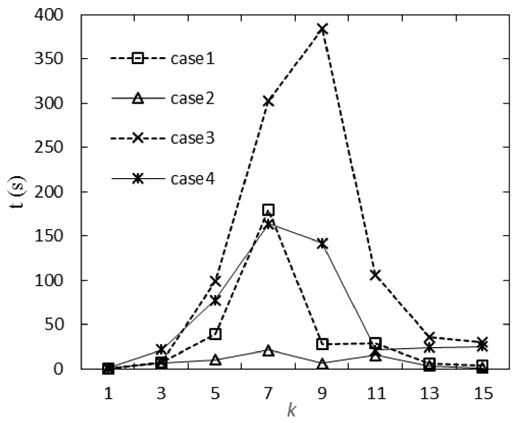
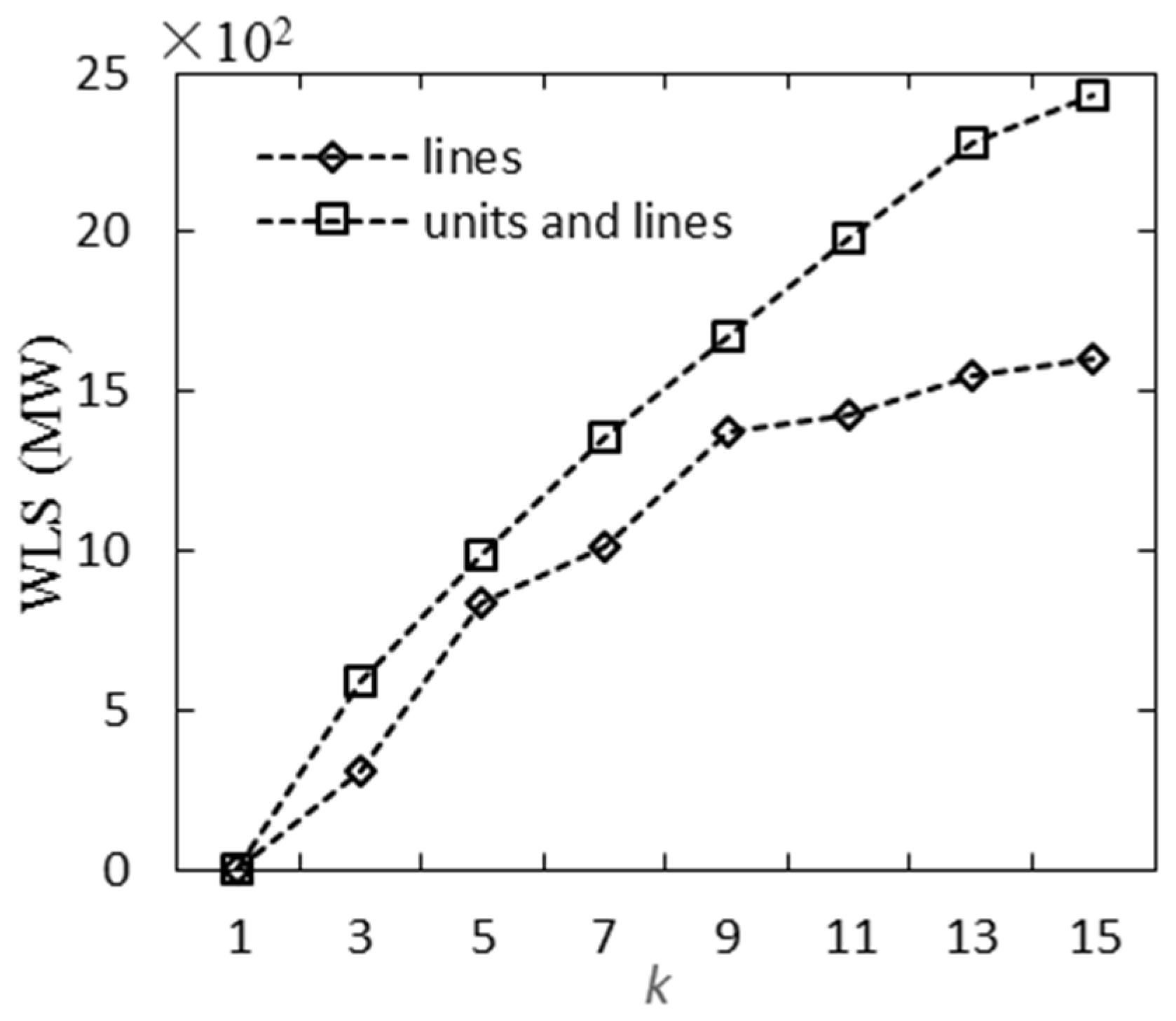
4.1. Results of Case 1 With Lines Contingecy and Peak Load

The minimum load shedding of the best system state is zero when the number of the lines out k equals to 1, 2, …, 23. Until k equals 24, the MLS of the best system state is 9 MW: respectively 5 MW at Bus 3 and 4 MW at Bus 19. The details of the contingency lines are 1–2, 1–3, 2–6, 3–24, 4–9, 5–10, 8–9, 8–10, 9–11, 10-11, 11–13, 11–14, 13–23, 15–21, 15–24, 16–17, 16–19, 17–18, 17–22, 18–21, 18–21, 19–20, 20–23, 21–23. The results of the best-case system state demonstrate some information. Under linearized DC power flow, zero load shedding may occur when 23 lines are out. The computational results of the best-case load shedding illustrate that load shedding must occur when k is larger than 23.

The computational results of WSS are provided in

Table 1. The computational results of the worst system state of case 1.

k	WLS/MW	Contingency Lines	t (s)
1	0	--	0.2
3	309	16–19, 20–23, 20–23	7.4
5	842	11–13, 12–13, 12–23, 14–16, 15–24	38.8
7	1017	1–3, 3–24, 7–8, 11–13, 12–13,12–23, 14–16	179.7
9	1373	7–8, 9–12, 10–12, 11–13, 15–21, 15–21, 16–17, 20–23, 20–23	27.9
11	1428	7–8, 9–12, 10–12, 11–13, 14–16, 15–16, 15–21, 15–21, 16–19, 20–23, 20–23	28.7
13	1552	1–3, 1–5, 2–4, 2–6, 7–8, 9–12, 10–12, 11–13, 15–21, 15–21, 16–17, 20–23, 20–23	5.8
15	1607	1–3, 1–5, 2–4, 2–6, 7–8,11–13, 12–13, 12–23, 14–16, 15–16, 15–21, 15–21, 16–19, 20–23, 20–23	3.1

WLS: The Worst Load Shedding; MW: Mega Watt.

. The first column of Table 1 is the number of lines out; the second column shows minimum load shedding, the third column gives the details of the contingency lines, and the last column is the computational time. For the sake of clear and representative expression, the values of k are, respectively, odd numbers from 1 to 15. When k = 1, WLS (MLS of WSS, also called worst load shedding) is zero, thus the outage of an arbitrary line doesn’t cause load shedding. When k = 3, WLS is 309 MW. These lines of the worst-case contingency are two lines between Buses 20 and 23, and Lines 16–19. The computational time increases by 179.7 s when k= 7. In fact, the optimization solver GUROBI6.0 found the optimal solution at 17 s, but the optimal gap is larger than 0.01%; until 179.7 s the gap is 0.0%. Other details are presented in Table 1.

4.2. Results of Case 2 With Lines Contingency and Interval Load

Table 2. The computational results of case 2.

k	WLS/MW	Contingency Lines	Non-Peak Buses	t (s)
1	0	--	--	0.2
3	309	16–19, 20–23, 20–23	7, 13	6.5
5	842	3–24, 11–13, 12–13, 12–23, 14–16	13, 19(1), 20	10.4
7	1017	2–4, 7–8, 11–13, 12–13, 12–23, 14–16, 15-24	7, 13(2), 18	21.1
9	1373	7–8, 11–13, 12–13, 12–23, 15–21, 15–21, 16–17, 20–23, 20–23	7, 13, 18	6.1
11	1428	7–8, 11–13, 12–13, 12–23, 14–16, 15–16, 15–21, 15–21, 16–19, 20–23, 20–23	7(2)	15.6
13	1552	1–3, 1–5, 2–4, 2–6, 7–8, 11–13, 12–13, 12–23, 15–21, 15–21, 16–17, 20–23, 20–23	1(1), 2	3.4
15	1607	1–3, 1–5, 2–4, 2–6, 7–8, 9–12, 10–12, 11–13, 14–16, 15–16, 15–21, 15–21, 16–19, 20–23, 20–23	1, 7, 18	1.1

presents the WSS results of Case 2. Because interval load is discretized by trisection for linearization, load demand at each load bus has four options: upper bound, the first value in interval, the second value in interval and lower bound. When WSS occurs, the load demand of most buses reaches the upper bound [8], but the load demand of little buses isn’t at peak load. In the fourth column of Table 2, the non-peak buses refer to these buses at which load demand isn’t at peak load when WSS occurs, and the numbers 1 and 2 in parentheses denote respectively the first value second values of the interval load. For load demand at Bus 1 for example, the interval load at Bus 1 ranges from 97 to 108 MW: 1 means the load demand is 97 MW, 1(1) means the load demand is 100.7 MW, and 1(2) means the load demand is 104.4 MW.

We compared the contents of Table 1 and Table 2, of which WLS are equal. Although their contingency lines and load demand are not the same in form, they are equivalent in essence. When k equals to 5, Lines 3–24 in Table 2 replaces Line 15–24 in Table 1, and the load at Bus 19 is the value 169 MW in interval load [163, 181] MW. We directly calculated the MLS retaining all condition except for the load at Bus 19 by linear programming. When the load demand at Bus 19 are, respectively, 163, 169 and 181 MW, their MLS are the same, all equal to 842 MW. The difference of the three conditions is only the output of a 155 MW generator at Bus 23, respectively, 17, 23 and 35 MW. The load demand at Bus 19 can be covered by generators around Load Bus 19, it has not impact on the WLS of N-k contingency. When k equals other number, the situations are the same as these above. In fact, the non-peak buses in Table 2 are also generation buses, except for Bus 19 and 20, which are close to the generation bus. When k = 7, Lines 2–4 and 15–24 in Table 2 replace Lines 1–3 and 3–24 in Table 1. When k = 9, 11, and 13, Lines 12–13 and 12–23 in Table 2 replace Lines 9–12 and 10–12 in Table 1, when k equals 15, otherwise as above. These comparison results demonstrate WSS model has the same optimum value but many solutions may exist.

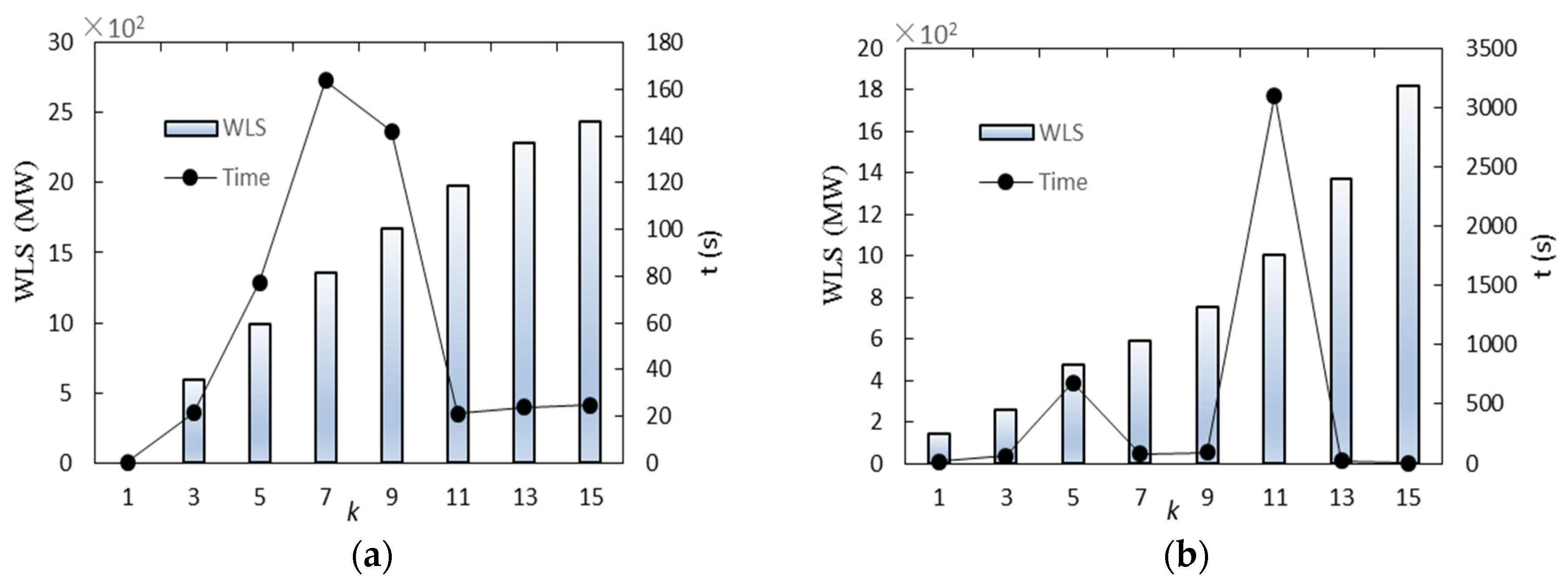
4.3. Results of Case 3 With Lines and Generators Contingency and Peak Load

The computational results of case 3 are presented in

Table 3. The computational results of case 3.

k	WLS/MW	Contingency Lines	Contingency Units/MW	t (s)
1	0	--	--	0.3
3	595	--	400(18), 400(21), 350(23)	7.3
5	989	--	2*197(13), 400(18), 400(21), 350(23)	98.9
7	1361	7–8	3*197(13), 400(18), 400(21), 350(23)	302.4
9	1671	7–8	3*197(13), 155(15), 155(16), 400(18), 400(21), 350(23)	384.4
11	1981	7–8	3*197(13), 155(15), 155(16), 400(18), 400(21), 2*155(23), 350(23)	105.7
13	2281	7–8, 17–22, 21–22	3*197(13), 155(15), 155(16), 400(18), 400(21), 2*155(23), 350(23)	35.2
15	2433	7–8, 17-22, 21–22	76(1), 76(2), 3*197(13), 155(15), 155(16), 400(18), 400(21), 2*155(23), 350(23)	30.5

, in which the fourth column provides the details of the contingency of generators of WSS, the number in parentheses denotes bus number, the value before symbol * represents the number of generator, for example, 2*197(13) refers to two 197 MW generators at Bus 13. When k= 1, the MLS is 0. IEEE-RTS-24 bus system meets the N-1 criteria, the outage of arbitrary lines or unit does not cause the load shedding. When k equals to 1, 3 and 5, the number of contingency lines of WSS is 0. These demonstrate the outage of generators have more impact than that of lines regarding to worst load shedding. When k equals to 7, 8 and 9, only one Lines 7–8 is out. When k equals to 13 and 15, there are the outage of three lines, they are Lines 7–8, 17–22 and 21–22. Note that in Table 3, the contingency lines of the third column include Lines 7–8, which is the weak region of IEEE-RTS-24 bus system.

We compared the worst load shedding of Table 1 and Table 3, as shown in Figure 2. The WLS with line and generator contingencies is more than that with only line contingencies, the difference value is 826 MW when k= 15. The N-k contingency analysis should consider the outage of the generator.

4.4. Results of Case 4 With Lines and Generators Contingency and Interval Load

The computational results of case 4 are presented in

Table 4. The computational results of case 4.

K	WLS/MW	Contingency Lines	Contingency Units/MW	Non-Peak Buses	t (s)
1	0	--	--	--	0.3
3	595	--	400(18), 400(21), 350(23)	7	21.4
5	989	--	2*197(13), 400(18), 400(21), 350(23)	--	77.3
7	1361	7–8	3*197(13), 400(18), 400(21), 350(23)	--	163.7
9	1671	7–8	3*197(13), 400(18), 400(21), 2*155(23), 350(23)	--	141.9
11	1981	7–8	3*197(13), 155(15), 155(16), 400(18), 400(21), 2*155(23), 350(23)	--	21.2
13	2281	7–8, 17–22, 21–22	3*197(13), 155(15), 155(16), 400(18), 400(21), 2*155(23), 350(23)	--	23.9
15	2433	7–8, 17–22, 21–22	2*76(2), 3*197(13), 155(15), 155(16), 400(18), 400(21), 2*155(23), 350(23)	--	24.9

. The only non-peak load bus is Load Bus 7 when k= 3. The comparison between Table 3 and Table 4 is similar to that between Table 1 and Table 2. However, the details of the contingency generators are different in this form, they are equivalent in essence. When k =9, two 155 MW generators at Bus 23 in Table 4 replace a 155 MW generator at Bus 15 and a 155 MW generator at Bus 16; when k equals to 15, a 76 MW generator at Bus 2 replace a 76 MW generator at Bus 1.

We compare the computation time for four cases, as shown in Figure 3. In case 3, when k= 9, the program uses the most time, 384.4 s. From the view of the contingency number, the consumption time is larger when k= 5, 7, 9, and 11. The consumption time is a normal distribution with the number of contingencies. The consumption time of these cases, considering the contingency of generators, is more than that without the contingency of generators. The computation time of the situation with interval loads is less than that with peak loads because of redundant constraints of the dual variables associated with the load demand.

4.5. Results of IEEE-118 Bus System With Lines and Generators Contingency and Interval Load

The IEEE-118 bus system consists of 186 lines, 54 generators and 99 load buses. The demand data in each load node are from the IEEE-118 bus case of Matpower [28], and the total peak demand is 4242 MW. Here, demand uncertainties are assumed as the range of ±5% of peak load. The generators data are from Reference [25] and the total generation capacity is 8270 MW. For other detailed data, please refer to References [25,28].

The worst load shedding of the N-k contingency of lines and generators with the interval load are calculated using the MILP method. The relative optimality gap of MILP is set 0.06 in GUROBI.

Table 5. The computational results of IEEE-118 bus system.

k	WLS/MW	Contingency Lines	Contingency Units/MW	t (s)
1	143.20	68–116	--	16
3	258.70	68–116, 77–78, 79–80	--	64
5	474.70	8–5, 13–15, 14–15, 16–17, 68–116	--	678
7	593.35	8–5, 15–17, 16–17, 15–19, 33–37, 68–116	100(15)	82
9	750.65	8–9, 23–24, 44–45, 42–49(2), 38–65, 68–116	500(8), 350(25)	92
11	1001.20	9–10, 81–80	500(8), 350(25), 250(46), 250(49), 200(56), 200(59), 420(62), 420(65), 300(66)	3101
13	1369.70	8–5, 86–87	300(24), 350(25), 250(46), 420(62), 420(65), 300(66), 500(77), 500(89), 300(92), 300(99), 300(100)	22
15	1819.70	8–5, 86–87	300(24), 350(25), 250(46), 250(49), 200(56), 420(62), 420(65), 300(66), 500(77), 500(89), 300(92), 300(99), 300(100)	4

and Figure 4b illustrate the computational results. Non-peak buses are not listed because all WSS occur at the upper bound of the interval load. The worst load shedding of N-1 is 143.20 MW. A 50 MW generator and 5% peak load 193.2 MW are at Bus 116, but Bus 116 is only connected to Bus 68 by one line, 68–116. Thus, the minimum load shedding is 143.20 MW (193.2–50) when Lines 68–116 are out. Thus, the IEEE-118 bus system does not meet N-1 standard. When k is less than 9, the worst load shedding average increases about 152 MW as two elements are added and the contingencies of the elements are mostly lines. When k is more than 9, the average absolute increased value is about 256 MW, and the contingency elements are mostly generators. Figure 4a also illustrates the worst load shedding and time of the IEEE-RTS-24 bus system in Section 4.4. The situation of the IEEE-118 bus system is different from that of the IEEE-RTS-24 bus system. In Table 4, for the IEEE-RTS-24 bus system, the contingency elements are mostly generators. Regarding to worst load shedding, the transmission system of the IEEE-RTS-24 bus system is more robust against the N-k contingency than the generation system. Meanwhile, the generation system of the IEEE-118 bus system is more robust than the transmission system.

The average consumption time of the worst load shedding by the MILP method is about 507 s in the IEEE-118 bus system; the average time is 59 s in the IEEE-RTS-24 bus system. With MILP optimization software being more mature, the computational time is very reasonable for large systems. Although the MILP method of searching for the worst load shedding consumes 3101 s when k is equal to 11 in Table 5, it has more advantages than the enumeration or screening methods. For the comparison between MILP and the complete enumeration method, we screened all N-k contingencies with certain loads, which are the same to that of the MILP method. The total number of elements of the IEEE-RTS-24 and IEEE-118 bus systems are, respectively, 66 (38 lines and 28 units) and 240 (186 lines and 54 units). The complete enumeration number of the N-k contingency is the combination number $C_N^k=\frac{N\text{!}}{k!*(N-k)!}$, which approximately increases exponentially with k increasing when the k value is less than the median number, from 1 to N. By testing these cases, only N-1, N-3, and N-5 of the IEEE-RTS-24 bus and N-1 and N-3 of the IEEE-118 bus systems can be finished in one day (24 h), their results about the worst load shedding are the same as that of the MILP method. Complete sampling is a very poor method for real power systems. Take N-3 of the IEEE-118 bus system for example, the number of enumerations is the combination number $C_{240}^3$, and the value is 2,275,280, the total consumption time is 47,174 s, which is larger than the 64 s in Table 5. The complete screening method is exponential time complexity, but the MILP method is polynomial time complexity because of the MILP algorithm using the branch and cut method. The MILP method is very applicable to the situation where k is more than 2. The advantage of MILP is that it directly identifies the worst scenario using the KKT optimization condition and strong duality theory.

5. Conclusions

The difficulty of N-k state analysis largely increases with increasing k when k is less than the median from 1 to N, thus, it is very difficult to identify the worst system state by complete screening. This paper provides a rigorous analytic method for identifying the worst state of N-k contingency of lines and generators with an uncertain load, which is a bi-level optimization problem. In order to efficiently solve the problem, strong duality equations and a mathematical linearization method are applied. An MILP method for identifying the worst scenario under uncertainties of N-k contingency and load demand was proposed. Numerical studies demonstrated the effectiveness of the method. The analytic method of the worst state of N-k contingency can be applied to the risk assessment of power systems, expansion planning, and unit commitment.

The models the paper proposed are based on linearized DC power flow. In the future, we will research analytic steady security with alternating current (AC) power flow, which is non-linear and non-convex. Prevention and correction of generators and network topology also have effects on the analytic security estimation, for example load shedding minimization by static var compensator or static synchronous compensator (SVC/STATCOM) [29]. The expansion and relaxation of simplifications and assumptions of the models will be carried out in future work.

References

1. Li, W. Risk Assessment of Power Systems: Models, Methods, and Applications; Wiley-IEEE: Hoboken, NJ, USA, 2005. [Google Scholar]
2. Karimi, E.; Ebrahimi, A. Probabilistic transmission expansion planning considering risk of cascading transmission line failures. Int. Trans. Electr. Energy Syst. 2015, 25, 2547–2561. [Google Scholar] [CrossRef]
3. Lee, S.T. Probabilistic online risk assessment of non-cascading and cascading transmission outage contingencies. Eur. Trans. Electr. Power 2008, 18, 835–853. [Google Scholar] [CrossRef]
4. Vaiman, M.; Keith, B.; Chen, Y.; Chowdhury, B.; Dobson, I.; Hines, P.; Papic, M.; Miller, S.; Zhang, P. Risk assessment of cascading outages: Methodologies and challenges. IEEE Trans. Power Syst. 2012, 27, 631–641. [Google Scholar] [CrossRef]
5. Youwei, J.; Ke, M.; Zhao, X. N-k Induced Cascading Contingency Screening. IEEE Trans. Power Syst. 2015, 30, 2824–2825. [Google Scholar]
6. Sing-Po, W.; Chen, A.; Chih-Wen, L.; Chun-Hung, C.; Shortle, J.; Jin-Yi, W. Efficient splitting simulation for blackout analysis. IEEE Trans. Power Syst. 2015, 30, 1775–1783. [Google Scholar]
7. Correa, C.A.; Bolanos, R.; Garces, A. Enhanced multiobjective algorithm for transmission expansion planning considering N-1 security criterion. Int. Trans. Electr. Energy Syst. 2015, 25, 2225–2246. [Google Scholar] [CrossRef]
8. Peng, W.; Haozhong, C.; Jie, X. The interval minimum load cutting problem in the process of transmission network expansion planning considering uncertainty in demand. IEEE Trans. Power Syst. 2008, 23, 1497–1506. [Google Scholar] [CrossRef]
9. Habibi, M.R.; Rashidinejad, M.; Zeinaddini-Meymand, M.; Fadainejad, R. An efficient scatter search algorithm to solve transmission expansion planning problem using a new load shedding index. Int. Trans. Electr. Energy Syst. 2014, 24, 153–165. [Google Scholar] [CrossRef]
10. Nam, H.K.; Kim, Y.H.; Shim, K.S.; Choi, J.H.; Kwak, N.H. A new ultra-fast contingency screening algorithm without time-domain simulation for online transient security assessment. Eur. Trans. Electr. Power 2008, 18, 725–741. [Google Scholar] [CrossRef]
11. Salam, M.A.; Ahmed, S.S. A new method for screening the contingencies before dynamic security assessment of a multimachine power system. Eur. Trans. Electr. Power 2006, 16, 393–408. [Google Scholar] [CrossRef]
12. Kaplunovich, P.; Turitsyn, K. Fast and Reliable Screening of N-2 Contingencies. IEEE Trans. Power Syst. 2016, 31, 4243–4252. [Google Scholar] [CrossRef]
13. Arroyo, J.M. Bilevel programming applied to power system vulnerability analysis under multiple contingencies. IET Gener. Trans. Distrib. 2010, 4, 178–190. [Google Scholar] [CrossRef]
14. Fliscounakis, S.; Panciatici, P.; Capitanescu, F.; Wehenkel, L. Contingency ranking with respect to overloads in very large power systems taking into account uncertainty, preventive, and corrective actions. IEEE Trans. Power Syst. 2013, 28, 4909–4917. [Google Scholar] [CrossRef]
15. Jiang, R.; Zhang, M.; Li, G.; Guan, Y. Two-stage network constrained robust unit commitment problem. Eur. J. Oper. Res. 2014, 234, 751–762. [Google Scholar] [CrossRef]
16. Arroyo, J.M.; Galiana, F.D. On the Solution of the Bilevel Programming Formulation of the Terrorist Threat Problem. IEEE Trans. Power Syst. 2005, 20, 789–797. [Google Scholar] [CrossRef]
17. Bard, J.F. Practical Bilevel Optimization: Algorithms and Applications, 1st ed.; Kluwer Academic Publishers: Dordrecht, The Netherlands, 1998. [Google Scholar]
18. Romero, N.R.; Nozick, L.K.; Dobson, I.D.; Xu, N.; Jones, D.A. Transmission and generation expansion to mitigate seismic risk. IEEE Trans. Power Syst. 2013, 28, 3692–3701. [Google Scholar] [CrossRef]
19. Zheng, Q.P.; Jianhui, W.; Liu, A.L. Stochastic optimization for unit commitment—A review. IEEE Trans. Power Syst. 2015, 30, 1913–1924. [Google Scholar] [CrossRef]
20. Majidi-Qadikolai, M.; Baldick, R. Stochastic Transmission Capacity Expansion Planning With Special Scenario Selection for Integrating N-1 Contingency Analysis. IEEE Trans. Power Syst. 2016, 31, 4901–4912. [Google Scholar] [CrossRef]
21. Pozo, D.; Sauma, E.E.; Contreras, J. A Three-Level Static MILP Model for Generation and Transmission Expansion Planning. IEEE Trans. Power Syst. 2013, 28, 202–210. [Google Scholar] [CrossRef]
22. Baringo, L.; Conejo, A.J. Transmission and wind power investment. IEEE Trans. Power Syst. 2012, 27, 885–893. [Google Scholar] [CrossRef]
23. Jin, S.; Ryan, S.M. A Tri-Level Model of Centralized Transmission and Decentralized Generation Expansion Planning for an Electricity Market—Part I. IEEE Trans. Power Syst. 2014, 29, 132–141. [Google Scholar] [CrossRef]
24. Subcommittee, P.M. Ieee reliability test system. IEEE Trans. Power Appl. Syst. 1979, PAS-98, 2047–2054. [Google Scholar] [CrossRef]
25. IEEE 118-Bus System. Available online: http//motor.ece.iit.edu/data/ (accessed on 20 October 2015).
26. Lofberg, J. Yamip. Available online: http://users.isy.liu.se/johanl/yalmip/ (accessed on 20 October 2015).
27. Gurobi Reference Manual. Available online: http://www.gurobi.com/documentation/ (accessed on 20 October 2015).
28. Matpower. Available online: http://www.pserc.cornell.edu/matpower/ (accessed on 20 October 2015).
29. Govind Singh, J.; Guha Thakurta, P.; Soder, L. Load curtailment minimization by optimal placements of SVC/STATCOM. Int. Trans. Electr. Energ. Syst. 2014. [Google Scholar] [CrossRef]
Figure 1. Model diagram.
Energies 10 00168 g001
Figure 2. Comparison of minimum load shedding of WSS.
Energies 10 00168 g002
Figure 3. Comparison of computation time.
Energies 10 00168 g003
Figure 4. WLS and consumption time of IEEE-RTS-24 and IEEE-118 bus system. (a) IEEE-RTS-24 bus system; (b) IEEE-118 bus system.
Energies 10 00168 g004