A Probabilistically Constrained Approach for the Energy Procurement Problem †

Department of Mechanical, Energy and Management Engineering, University of Calabria, via P. Bucci 41/C, 87036 Rende (CS), Italy
*
Author to whom correspondence should be addressed.
†
This paper is an extended version of our paper published in Energy Procedia: A multi-objective unit commitment problem combining economic and environmental criteria in a metaheuristic approach. Energia Procedia, 2017, 136, 283–289.
Energies 2017, 10(12), 2179; https://doi.org/10.3390/en10122179
Submission received: 13 November 2017
/
Revised: 10 December 2017
/
Accepted: 15 December 2017
/
Published: 19 December 2017
(This article belongs to the Special Issue Selected Papers from ICEER 2017: 2017 the 4th International Conference on Energy and Environment Research)
Abstract
:The definition of the electric energy procurement plan represents a fundamental problem that any consumer has to deal with. Bilateral contracts, electricity market and self-production are the main supply sources that should be properly combined to satisfy the energy demand over a given time horizon at the minimum cost. The problem is made more complex by the presence of uncertainty, mainly related to the energy requirements and electricity market prices. Ignoring the uncertain nature of these elements can lead to the definition of procurement plans which are infeasible or overly expensive in a real setting. In this paper, we deal with the procurement problem under uncertainty by adopting the paradigm of joint chance constraints to define reliable plans that are feasible with a high probability level. Moreover, the proposed model includes in the objective function a risk measure to control undesirable effects caused by the random variations of the electricity market prices. The proposed model is applied to a real test case. The results show the benefit deriving from the stochastic optimization approach and the effect of considering different levels of risk aversion.
1. Introduction
In recent years, commercial and industrial businesses are actively looking for effective ways to reduce energy usage and associated costs. Besides the shared concern towards the dramatic climate changes that has been leading governments to promoting the deployment of renewable energy technologies [1], the reduction of electricity costs represents a key factor to survive and compete in a global marketplace.
In this paper, we analyze the problem faced by a large consumer, equipped with a limited self-production facility, who has to define the optimal electric energy procurement plan over a given time horizon. The same problem, here further investigated, has been addressed by the authors in [2] (the present contribution is an extension of a conference paper that appeared in Energia Procedia, vol. 136, pp. 283–289, 2017). Referring to future time, the procurement process is clearly affected by uncertainty, mainly related to the electricity prices and demands which are unknown when the commitment decisions should be undertaken. Uncertainty in electricity prices can be dealt, in principle, by using two approaches. The first one is related to the demand response programs (see, for example, [3,4]), which, however, can not be applied in the case of production processes with a limited flexibility.
The second one relies on bilateral contracts, i.e., agreements signed in advance with pre-defined unit prices. In this case, the risk associated with price variation is absent, but the procurement costs are typically higher. Moreover, power contracts require the consumer to commit far in advance the amount to purchase for a given time period. The decision to purchase electricity from the market can be taken in a shorter term, one day in advance or even less (i.e., real-time), but this flexibility carries on the risk of increased volatility. It is evident that only a perfect mix of the procurement alternatives (self-production, bilateral contracts, and energy market) can provide the best results. The problem is made much more challenging by the presence of uncertainty that can not be ignored. Indeed, solutions based on deterministic estimates can result in infeasible procurement plans due to stochastic demands and/or to high costly and risky strategies.
This paper proposes the use of the chance constraints paradigm to address the procurement problem under uncertainty. Dating back to Charnes and Cooper [5], chance constraints represent and old but still modern topic in optimization, used to model many problems arising in the energy sector (see, for example [6,7,8,9,10]). The main idea is to “relax” the stochastic constraints, requiring their satisfaction with a predefined reliability value. The chance constraint paradigm belongs to the more general framework of stochastic programming (see, the textbooks [11,12]), but, differently from the recourse strategies, it has not been used to model stochastic procurement problems.
We note that the scientific literature on the procurement problem analyzed from a consumer’s perspective is quite limited. Much more papers address the problem from an electricity producer’s point of view (see, for example, [13,14,15] and the references therein). Conejo et al. [16] solve a deterministic procurement problem over a medium-term time horizon. The model considers a set of bilateral contracts, hourly changing spot prices and the possibility of self-producing energy. In a subsequent work [17], the authors address a similar problem for a shorter time horizon and accounts for cost volatility by an estimate of the covariance of the spot price.
While the contributions propose deterministic approaches, uncertainty affecting model parameters is accounted in [18] by the use of an Analog Ensemble approach. This technique provides reliable and bias-calibrated forecasts to include into the optimization problem. Much more related to our approach is the contribution by Carrion et al. in [19] who apply the stochastic programming framework, but in the form of multistage, to address the procurement problem over a medium-time horizon. The uncertain evolution of the day-ahead electricity price is represented by a scenario tree and stage-wise decisions refer to the amount to purchase from the market and self-production that, unlike the commitment from the bilateral contracts, can be deferred in time. The model also includes a risk measure, the Conditional Value at Risk (CVaR), which is used to evaluate the clear trade-off between expected cost and risk. A similar trade-off is also investigated by Zare et al. [20] by the use of the information gap theory with the aim of evaluating the robustness of the solutions against high spot prices or high procurement costs. Beraldi et al. propose in [21] a recourse two-stage formulation for the procurement problem over a short-term planning horizon. The problem is solved in a rolling-horizon fashion using each time the more updated information. More recently, Beraldi et al. [22] analyze the procurement problem from the perspective of an aggregator, seen as the entity responsible to manage the distributed energy resources shared within a coalition, and propose a multi-period two-stage stochastic programming formulation.
The present contribution represents an extension of the conference paper presented at the International Conference on Energy and Environmental research (ICERRR), Porto 2017, and appeared in [2]. With respect to the referred scientific literature, the paper proposes the adoption of the paradigm of chance constraints to deal with the uncertainty clearly affecting the load profile to define a reliable procurement plan. Moreover, the proposed approach accounts for the volatility in the market prices by a mean-risk approach, optimizing the weighted sum of the expected cost and a risk measure represented by the CVaR. In this way, by varying the weighting factor, different procurement plans, reflecting a different aversion towards risk, may be derived to provide the decision maker with different strategies to evaluate also on the basis of his experience. With respect to the conference paper [2], the proposed approach is refined and additional computational experiments have been carried out to further investigate the validity of the approach also on the basis of an out-of-sample analysis.
The rest of the paper is organized as follows. Section 2 introduces the problem and presents the stochastic programming model. Section 3 presents the reformulation of the problem under the assumption of discrete random variables. Section 4 reports on the computational experiments carried out to investigate the validity of the proposed approach on a real test case. Section 5 discusses the main findings on the basis of the collected results and recommended managerial insights. Finally, concluding remarks and future research directions are summarized in Section 6.
2. Problem Statement and Formulation
We consider the problem faced by a large consumer who has to define the optimal procurement plan to satisfy the electric energy needs over a given time horizon. We denote by the set of periods of the planning horizon, indexed by t, and we assume that the consumer has a self-production facility of limited capacity (e.g., a cogeneration unit and/or a renewable energy system) that can be used to partially cover the energy demand. The main supply options that the prosumer (i.e., the consumer acting also as producer) has to evaluate are represented by the bilateral contracts and electricity market. We denote by the set of potential bilateral contracts. For each contract , the consumer has to decide in advance the amount to commit for each time period t. We denote by a binary decision variable related to the selection of the contract i and by the amount to purchase from contract i at the time period t. We let this latter variable depend on the time-of-use f to represent the most general situation experienced in many electricity market where a price variation is registered in the different hours of the day. For example, in Italy, three time-of-use blocks are considered: peak, intermediate and off-peak. We denote by the corresponding set, indexed by f. The price of bilateral contracts is pre-defined in advance when the agreement is signed. For generality, we also consider a fixed cost, denoted by , to account for all administrative expenses.
Electricity market represents the other supply alternative to take into account when defining the procurement plan. We denote by the amount of energy to purchase in the Day-Ahead Electricity Market (DAEM) for each time period t and block f. We also add, for generality, the decision variables denoting the amount of energy to eventually sell, if leftover, to the market. The market purchasing and selling prices are not known in advance since many factors contribute to their variation. We assume that these prices are random variables defined on a given probability space and we use the dependence on to denote their random nature. Thus, we denote by and the purchasing and selling prices, respectively. Besides prices, also the energy needs are unknown when the procurement decisions should be taken. We denote by the random electricity requirement for the period t and time-of-use block f.
For generality, we also consider a set of decision variables related to the self production. In particular, we denote by the amount to produce at period t and time block f. Moreover, we indicate by the upper bound on the production capacity and by the unitary production cost. Appendix A reports the full list of symbols.
The random nature of some of the parameters involved in the decision process calls for the definition of an optimization model explicitly accounting for the stochastic constraints and objective function.
2.1. Constraints
The proposed model includes stochastic and deterministic constraints. The first ones are related to the satisfaction of the random demand over the entire planning horizon. We deal with these constraints by adopting a reliability approach to define a procurement plan robust enough to hedge against unfavorable events that may occur in the future. We observe that the commitment decisions should be taken in advance without knowing the exact demand profile. A conservative approach would suggest to take as reference the worst-case situation that may occur, accepting to incur a cost unnecessary high. Conversely, using an average demand profile might result in an infeasible procurement plan if the realized demands are higher than estimated average ones. In such a case, the recourse to the balancing market is required to fulfill the demands, but with much higher costs. Chance constraints provide the way to mathematically translate the position of a decision maker who is willing to accept a shortage in the demand satisfaction as long as this event occurs only with a limited probability value. Thus, the procurement plan is defined to satisfy the following constraints:
Here, the parameter reflects the decision maker attitude towards the risk of shortage. Clearly, the higher the value the safer, but more expensive, the suggested procurement plan. We observe that Equation (1) represents the joint form of the classical chance constraints formulation: they jointly require the satisfaction of the demand for all the periods and time-of-use blocks rather than imposing many single chance constraints for each period and time block combination. The satisfaction of single chance constraints with a given confidence level does not necessarily guarantee the joint satisfaction of the constraints with the same reliability value.
The definition of a feasible procurement plan is also limited accordingly the next deterministic constraints:
Constraints in Equation (2) limit the amount of energy that the consumer might self-produce. This amount limits, in turn, the amount of energy that the consumer might sell to the market (Equation (3)). Constraints in Equations (4) and (5) are related to the bilateral constraints. In particular, we impose a limit K on the maximum number of contracts that can be selected. For each selected contract i, Equation (5) imposes a lower () and upper bound () on the amount of energy that can be purchased. Finally, constraints in Equations (7) and (8) state the nature of the decision variables.
2.2. Objective Function
The optimal plan should be defined to minimize the overall procurement cost . The straightforward way to deal with the random cost is to consider the expected value. In this case, the objective function assumes the following form:
Here, the first term represents the cost for self-producing energy, the second one quantifies the amount paid to purchase electricity from the bilateral contracts, and the last term accounts for the market expenses. The revenue deriving from the sale, if any, is accounted with the opposite sign.
Expected value indicates a neutral risk position. However, minimizing the average cost in the long run may not always be the right choice from a practical perspective since several and high variations in the market prices may have a strong negative effect on the consumer’s financial state. Under uncertain market conditions, minimizing a risk measure could be an important issue to evaluate and properly integrate in the model. There are many risk measures widely used in practice, such as variance, shortfall probability, downside risk, Value at risk (VaR). We refer the interested readers to the survey paper [23] and the references therein. In this paper, we choose as risk measure the CVaR.
For a given (0,1), the is defined as the expected loss greater than the -quantile of the loss distribution (VaR). Since its introduction by Rockafeller and Uryasev [24], the CVaR has become very popular because of its ability to consider the probability density in the tail of the distribution, its mathematical properties of being a coherent risk measure [25], and the ease of incorporation in stochastic optimization model. In our problem, we consider the cost distribution and we focus on the right tail, considering costs having a higher value of the -quantile of the cost distribution. Thus, the CVAR for a given confidence level is defined according to the following equation:
Figure 1 represents the CVaR in terms of costs.
Our model integrates expect cost and risk by a bi-objective given approach according to the expression:
The weighting factor can be used to specify which objective should be more emphasized. The smaller is , the more risk averse is the solution, since a higher weight is assigned to the CVaR. If , only the CVaR is considered. On the contrary, when is set to 1, a risk-neutral position is modeled. By varying , different plans reflecting a different aversion towards risk may be derived to provide the decision maker with different strategies to evaluate based on his experience and knowledge of the application domain.
3. Dealing with Joint Chance Constraints and Risk
The proposed model belongs to the class of mixed-integer problems under joint chance constraints and integrates in the objective function the CVaR risk measure. In what follows, we show how to deal with this problem when discrete random variables are considered. We point out that the assumption on the nature of the random variables is quite general. Many random variables are discrete by nature or are approximated as discrete ones (by taking, for example, a Monte Carlo sample from a general distribution) to overcome the difficulties related to the solution of multidimensional integrals. The discrete nature of the random variables and of some of the decisions variables (those related to the selection of the contracts) makes the problem very challenging. The study of the scientific literature shows that there is an increasing attention towards this class of problems, with much emphasis on the definition of solution approaches, both exact and approximate. We refer the interested readers to [26,27,28] and the references therein.
From now on, we shall assume that the discrete random variable can take a set of possible realizations. For all the random variables, we use the superscript s to refer to the generic realization s and we denote by the corresponding probability of occurrence. In this case, the probabilistic constraints in Equation (1) can be reformulated (see, for example, [29]) according to the expressions:
where are scenario dependent binary support variables and denotes the demand for the time period t and block f under scenario s. Obviously, the number of scenarios affects the computational tractability of the deterministic equivalent problem, calling for the definition of solution methods that exploit the specific problem structure. We have empirically found that, for the considered test case, the solution times required by off-the-shelf software are still affordable for a moderate size of the scenario set. The design of tailored solution methods is the subject of ongoing research.
We now turn to reformulate the . Under the assumption of discrete distribution function, this risk measure can be rewritten as:
where the represents the -quantile of the cost distribution and denotes the maximum value between 0 and . This last term can be rewritten using the support variables defined in the following expressions:
The term represents the cost under scenario s and it is defined by considering the scenario realization of the purchasing and selling prices accordingly to the following equation:
whereas represents a free decision variable.
4. Computational Results
This section is devoted to the presentation and discussion of the computational experiments carried out to evaluate the proposed decision approach. We have considered a real case study consisting in the definition of the procurement plan for the University of Calabria (UNICAL), Italy. With 12 Departments and about 34,000 students, 900 teachers, 760 technical and administrative staff, UNICAL is classified as medium size university with an average annual demand of 20 GWh. The campus has a limited self-production capacity deriving from a conventional production system with a nominal power of 2 MW and a set of small photovoltaic (PV) power plants, whose production reduces the energy demand.
We have considered a time horizon of one year divided in elementary monthly periods. Following the structure of the Italian market, we have considered three time-of-use blocks: peak (F1), intermediate (F2) and off-peak (F3). We have considered a set of 10 bilateral contracts and we have fixed to 8 the value of the parameter K. Table 1 reports the average unit price for each time-of-use block and the fixed costs. The overall set of data, also including the lower and upper bounds on the bilateral contracts are reported in Appendix B.
The preliminary step to the model solution is the generation of the required input data. Market price values have been derived by using a Monte Carlo simulation technique, based on a mean reverting process [30]. The choice of this approach has been motivated by the need of taking into account both seasonal effects and tendency of spot market prices to fluctuate around a drift over time. Figure 2 shows the different scenarios for the market price for the time-of-use block F1.
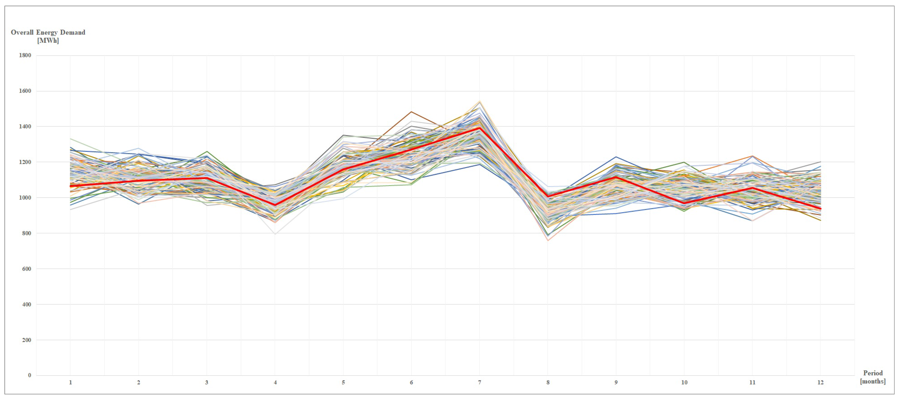
The red line represents the real profile, that as evident, falls within the scenario set. As for the load scenarios (shown in Figure 3), starting from the available historical data, we have determined the average values, properly reduced by the production from renewable systems, and then we have applied random variations within a predefined range. Energy demands have been considered independent from the market prices and the overall scenario set has been obtained by merging the single scenario sets through the Cartesian product. Then, a scenario reduction technique has been adopted ([31,32]) to deal with computationally tractable problems. The results reported hereafter refer to a set of 500 scenarios.
The proposed approach has been implemented in MATLAB (MathWorks, Inc., Natick, MA, USA) as for the scenario generation and GAMS 24.7.4 (GAMS Development Corporation, Fairfax, VA, USA) as algebraic modeling system, with CPLEX 12.6 (Ibm Corporation, Armonk, NY, USA) as solver. All the experiments have been carried out on a PC Intel Core I5 (2.3 GHz) with 4 GB of RAM DDR3. The solution times are quite short and have not been reported.
Several experiments have been carried out to fully investigate the performance of the proposed approach and to provide managerial insights on the optimal procurement strategies derived as function of the reliability level () and the risk aversion attitude (). In the following subsections, we present and discuss the results of a broad sensitivity analysis study. We point out that the presented results have been carried out by considering a value of equal to 0.95. Quite similar results have been also obtained for other values of and are not reported here, since no considerable variation in the solutions has been registered.
4.1. The Impact of the Reliability Level
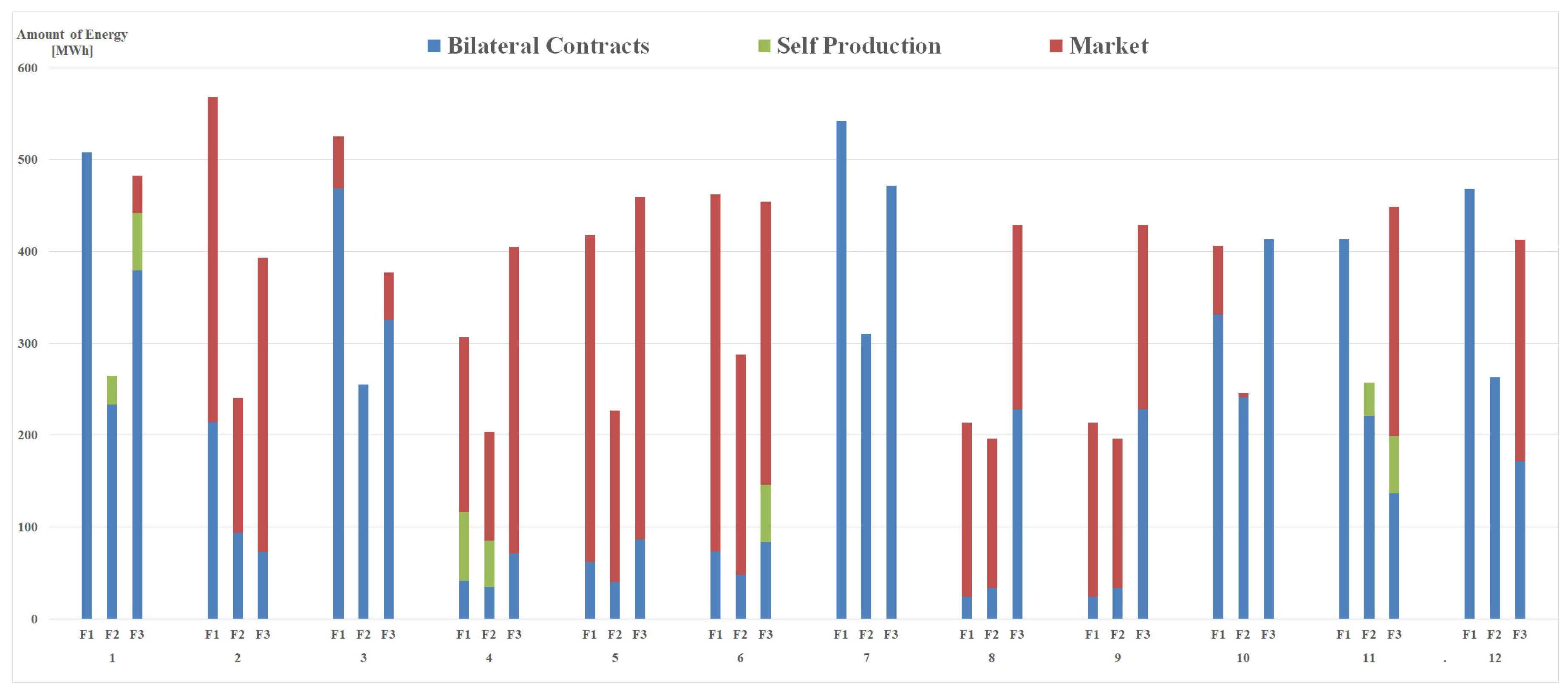
We have tested the model for different levels of the reliability value . Figure 4 reports the results for a given choice of the weight set equal to 0.5 and a reliability value equal to 0.95.
As evident, the optimal plan suggests different combinations of the supply sources for the different time periods of the planning horizon. For example, for some months, the amount procured from bilateral contracts is higher than the quantity purchased from the market. By varying the value, the decision maker can mathematically express a more concerned position towards the demand satisfaction. The extreme case of equal to 1 translates an overconservative position, requiring the constraint satisfaction for every possible demand profile. Clearly, safer plans are more expensive, as shown in Table 2, which reports the average costs and the CVaR values as function of .
Looking at the results, we may observe the increase in the expected cost as passes from 0.85 to 1. We note that, as expected, the CVaR values are always greater than the expected cost ones, since they measure the expected cost in the of the worst case realizations (i.e., higher costs).
There is clearly a trade-off between cost increase and reliability that the decision maker may be willing to evaluate. Under this respect, the proposed model provides a tool to support the decision-maker to choose the best combination.
4.2. The Effect of the Risk Modeling
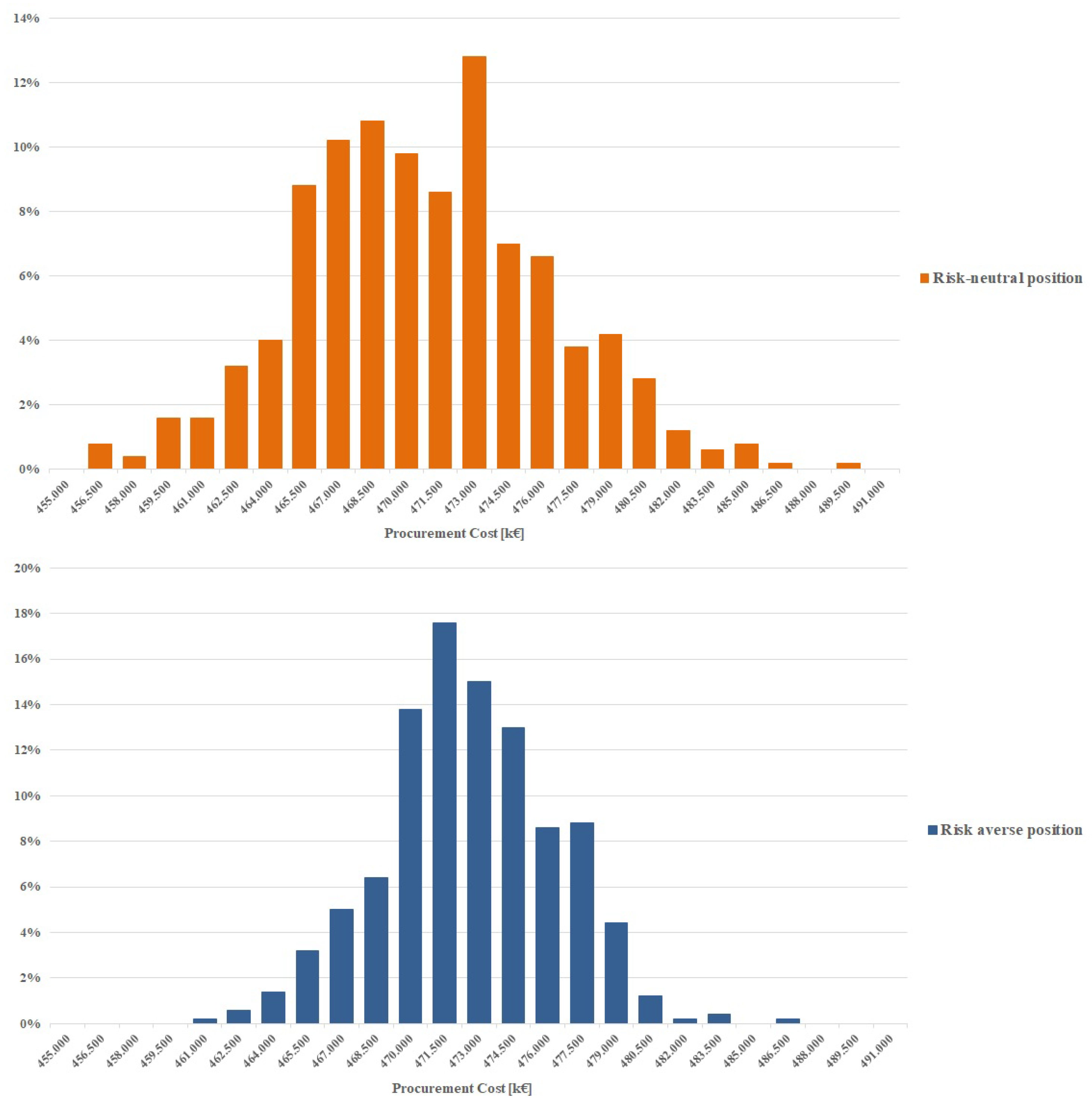
Other experiments have been carried out to analyze the effect produced by the choice of the weight in the definition of procurement plan for a fixed reliability value. Figure 5 shows the cost distribution for fixed level of and equal both to 0.95 and two different values of representative of a total risk aversion () and risk-neutral () position.
As evident from the results, when a total risk-averse position is considered, the cost distribution tightens because the decision-maker focuses on reducing the possibility of incurring high procurement costs. In this case, we may note an increase of the expected cost and a reduction of the possibility of bearing lower costs.
On the contrary, when a risk-neutral position is considered, the cost distribution is more dispersed. The decision maker is interested in minimizing the expected cost, accepting the possibility to experience higher costs in a given percentage of possibilities.
Figure 6 shows the relation between expected costs and the CVaR for different values.
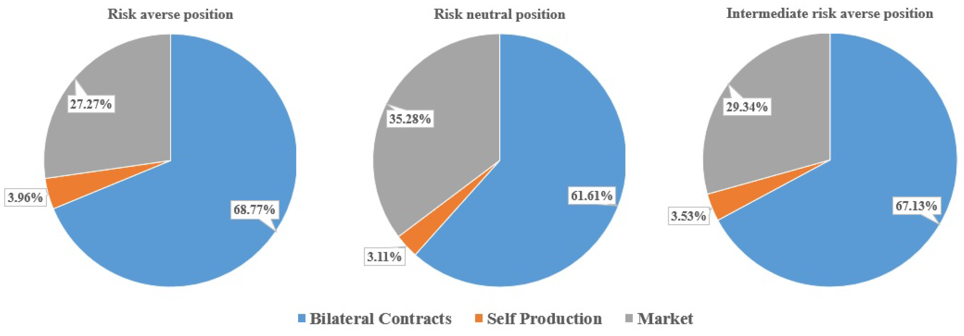
The results confirm that in order to reduce the CVaR, higher expected costs are incurred. Figure 7 indicates the change in the procurement costs, evaluated on the basis of the average market costs, for varying level of risk aversion.
The results (obtained for ) reveal that the percentage of costs related to the bilateral contracts tends to decrease when we reduce (by ) the level of the risk aversion. As expected, the results suggest that a higher level of risk awareness leads to the definition of plans that privilege the bilateral contracts as procurement alternative, whereas, in the case of risk-neutral position, the recourse to the market is increased.
4.3. Out-of-Sample Analysis
Additional experiments have been carried out to evaluate the application of the proposed approach as decision support system in a real setting. To this aim, we have evaluated the proposed plans by considering the real evolution of the market prices and demand requirements. First, we observe that the deterministic model, solved by considering the expected values of the unknown parameters, does not provide a feasible plan when considering the observed values of the energy profile. On the contrary, the proposed approach provides feasible solutions for the different values of tested. For some periods and time-of-use blocks, the real demand is lower than the -quantile used in the deterministic reformulation and, thus, the decision maker may decide to sell to the market the amount in excess realizing some profit. Table 3 reports the results for equal to 0.90 and different values of . Similar results have been also obtained for the other configurations of the parameters.
Looking at the results presented in terms of costs, we may observe that in the case of a risk-averse position, the amount spent for purchasing energy from bilateral contracts and self producing energy is higher. In this case, however, reselling the amount in excess determines a reduction of the costs related to the market (in some cases also a profit represented with the sign minus in the table). Overall, the proposed solutions provide balanced plans in terms of real costs spent to cover the real demand. This conclusion is confirmed by the results collected when solving the problem on the observed realization of the uncertain parameters. In this case, the optimal procurement cost is 334,276.51€. Comparing this value with the cost of the proposed procurement alternatives , we may observe that the maximum saving is around 1.2%. This low value confirms the validity of the proposed approach as proper support to define robust procurement strategies applicable in a real setting.
Moreover, some more experiments have been carried out in order to compare the solutions, in the out-of-sample fashion, provided by the proposed approach w.r.t. those obtained by adopting the approach in [22]. Here, the problem is solved by means of a multi-period two-stage stochastic programming problem, with recourse variables representing the energy amounts to buy/sell on the market in order to guarantee the energy balance. The model has a similar mean-risk objective function structure, again with the CVaR as risk measure. Table 4 shows the overall cost for different values of the risk aversion parameter of the two-stage model (2S) and the chance constraint approach (CC).
As expected, the greater flexibility guaranteed by the chance constraint formulation allows obtaining less expensive procurement plans, even in a real-life operative context.
5. Discussion
The results from the real case study show the effectiveness of the proposed approach as a tool for supporting the decision maker in defining the best procurement plan under demand and market price uncertainty. The introduction of the chance constraints and the CVaR allows to jointly investigate and control the effects produced by the two sources of uncertainty and risk. Based on the results, collected on a real test case, some considerations can be drawn.
First, we observe that by varying the reliability level , it is possible to generate different procurement plans that reflect a different concern towards the demand satisfaction, ranging from more prudent to riskier positions. The necessity of accounting for demand uncertainty is confirmed by the results carried out on the out-of-sample analysis. Indeed, the procurement plan determined when solving a deterministic model, with the expected value of the random demand profile, results infeasible when implemented on the real data. In this case, expensive corrective actions, involving the purchase of energy on the balancing market, must be undertaken to guarantee the demand satisfaction.
Obviously, safety has a price, as highlighted by the increase in the objective function value. Once fixed a proper reliability level, the decision maker may evaluate how the weight attributed to the risk can impact on the suggested plan. The volatility of the market prices generates fluctuations of the overall procurement costs. Risk averse decision makers are willing to minimize the risk measure to provide procurement strategies which are less sensitive to the price variation. In this case, the expected cost can be higher, but the possibility of incurring high procurement costs is reduced. On the contrary, risk-neutral position aims at minimizing the expected cost only, leaving aside what happens in the tail of the cost distribution.
The most remarkable insight drawn from the analysis of the overall results is that, to determine solutions that can be applied in a real setting, uncertainty should definitely be incorporated into the optimization process. The additional comparison with a recourse based stochastic programming approach confirms the effectiveness of the chance constrained formulation and seems to provide, at least on the considered case study, slightly better results. Under this respect, the proposed approach can be seen as a valuable tool to support the decision maker in identifying the best procurement strategy.
6. Conclusions and Future Research Directions
In this paper, the energy procurement problem under uncertainty is modeled by integrating the paradigm of joint chance constraints and the CVaR risk measure. Bilateral contracts, energy market and self-production are the main supply sources that should be properly combined to satisfy the energy profile and minimizing the overall costs. The proposed approach helps the decision maker to identify the procurement strategy and evaluate its robustness against variation in the demand and market prices. The results shows the validity of the proposed approach when implemented on a real case study. We point out that the definition of the amount to purchase from bilateral contracts is preliminary to the problem that a consumer, eventually integrated within a coalition, should solve to optimally manage the available resource on a short-term planning horizon. The integration of the procurement and management problems within a decision support tool is the subject of the ongoing research [33].
Acknowledgments
This work has been partially supported by Italian Minister of University and Research with the grant for research project PON03PE_00050_2 “DOMUS ENERGIA - Sistemi Domotici per il Servizio di Brokeraggio Energetico”.
Author Contributions
The work presented in this paper is a collaborative development by all of the authors. P.B. and M.E.B. contributed with the analysis of the scientific literature and the definition of the stochastic programming formulations; A.V. analysed the case study and designed the implementation of the proposed models; G.C. ran all the computational experiments. All authors contributed to the organization of the paper including writing and proofreading.
Conflicts of Interest
The authors declare no conflict of interest.
Appendix A. Nomenclature
In Table A1, we report the main symbols used in the paper.

Table A1.
Main symbols.
| Nomenclature | |
|---|---|
| Sets | |
| set of elementary time periods (months) | |
| F | set of time-of-use blocks in which hours are divided |
| set of potential bilateral contracts | |
| S | set of scenarios used for representing evolution of uncertain parameters |
| Deterministic Parameters | |
| unit energy price of bilateral contract i for time-of-use block f of time period t (€/MWh) | |
| fixed cost for selection of bilateal contrat i (€) | |
| confidence level for chance constraints | |
| confidence level for Conditional Value at Risk | |
| K | maximum number of active bilateral contracts |
| upper bound on the energy amount that can be produced in time-of-use block f | |
| of time period t (MWh) | |
| lower and upper bound on the quantity that can be bought from bilateral contract i | |
| in time-of-use block f of time period t (MWh) | |
| production cost for time-of-use block f of time period t (€/MWh) | |
| probability of occurrance of scenario s | |
| Stochastic Parameters | |
| overall energy demand for time-of-use block f of time period t under scenario s ([MWh]) | |
| unit purchasing price on day-ahead market for time-of-use block f of time period t | |
| under scenario s (€/MWh) | |
| unit selling price on day-ahead market for time-of-use block f of time period t | |
| under scenario s (€/MWh) | |
| Decision Variables | |
| selection of contract i | |
| amount of energy to purchase by bilateral contract i in time-of-use block f | |
| of time period t (MWh) | |
| amount of energy to buy from the day-ahead market in time-of-use block f | |
| of time period t (MWh) | |
| amount of energy to sell on the day-ahead market in time-of-use block f | |
| of time period t (MWh) | |
| amount of energy to produce in time-of-use block f of time period t (MWh) | |
| Auxiliary Variables | |
| auxiliary variable for CVaR linearization | |
| auxiliary variable for chance constraints linearization | |
| scenario dependent binary support variables | |
| Dependent Variables | |
| overall cost under scenario s | |
| Value at Risk for a certain confidence level (€) | |
| Conditional Value at Risk for a certain confidence level (€) | |
Appendix B. Bilateral contracts
Table A2, Table A3 and Table A4 report the complete characteristics of the bilateral contracts considered for the computational experiments.
Table A2.
Bilateral contracts unit price (€/MWh) and fixed cost (€).
| Bilateral Contracts | 1 | 2 | 3 | 4 | 5 | 6 | 7 | 8 | 9 | 10 | |
|---|---|---|---|---|---|---|---|---|---|---|---|
| January | F1 | 42.27 | 44.38 | 35.51 | 41.90 | 41.42 | 39.35 | 39.35 | 41.32 | 43.39 | 49.89 |
| F2 | 43.27 | 34.62 | 36.35 | 42.89 | 42.41 | 46.22 | 48.53 | 55.81 | 44.65 | 35.72 | |
| F3 | 35.77 | 42.21 | 33.77 | 35.46 | 35.06 | 41.02 | 43.07 | 34.45 | 39.62 | 40.81 | |
| February | F1 | 42.27 | 40.16 | 44.17 | 48.59 | 41.42 | 45.57 | 50.12 | 47.62 | 45.24 | 49.76 |
| F2 | 43.27 | 47.60 | 45.22 | 49.74 | 42.41 | 46.65 | 44.31 | 48.75 | 53.62 | 58.98 | |
| F3 | 35.77 | 39.35 | 43.28 | 41.12 | 35.06 | 38.56 | 36.63 | 40.30 | 44.33 | 47.43 | |
| March | F1 | 42.27 | 41.42 | 41.42 | 37.28 | 41.42 | 41.42 | 37.28 | 36.54 | 35.80 | 32.22 |
| F2 | 43.27 | 43.27 | 42.41 | 38.17 | 42.41 | 38.17 | 37.40 | 33.66 | 33.66 | 33.66 | |
| F3 | 35.77 | 32.20 | 32.20 | 31.55 | 35.06 | 31.55 | 30.92 | 30.92 | 27.83 | 24.49 | |
| April | F1 | 42.27 | 41.85 | 43.94 | 43.94 | 41.42 | 43.49 | 43.49 | 43.06 | 42.63 | 42.63 |
| F2 | 43.27 | 45.44 | 44.98 | 44.98 | 42.41 | 42.41 | 41.98 | 41.98 | 44.08 | 46.29 | |
| F3 | 35.77 | 35.77 | 37.56 | 37.19 | 35.06 | 35.06 | 34.71 | 36.44 | 36.44 | 34.98 | |
| May | F1 | 42.27 | 43.54 | 44.84 | 47.08 | 41.42 | 42.67 | 44.80 | 46.14 | 47.53 | 49.90 |
| F2 | 43.27 | 44.57 | 45.91 | 48.20 | 42.41 | 44.53 | 45.86 | 48.16 | 49.60 | 51.09 | |
| F3 | 35.77 | 37.56 | 38.69 | 39.85 | 35.06 | 36.81 | 37.91 | 39.05 | 41.00 | 43.46 | |
| June | F1 | 42.27 | 43.11 | 42.25 | 42.25 | 41.42 | 40.59 | 40.59 | 41.41 | 42.23 | 42.23 |
| F2 | 43.27 | 42.41 | 43.25 | 43.25 | 42.41 | 42.41 | 43.25 | 43.25 | 42.39 | 41.54 | |
| F3 | 35.77 | 35.77 | 35.06 | 35.76 | 35.06 | 35.06 | 35.76 | 35.04 | 35.04 | 35.74 | |
| July | F1 | 42.27 | 42.27 | 35.93 | 28.74 | 41.42 | 35.21 | 28.17 | 28.17 | 28.17 | 22.53 |
| F2 | 43.27 | 36.78 | 36.78 | 29.42 | 42.41 | 33.93 | 33.93 | 27.14 | 23.07 | 19.61 | |
| F3 | 35.77 | 28.62 | 24.33 | 24.33 | 35.06 | 28.05 | 28.05 | 23.84 | 19.07 | 17.55 | |
| August | F1 | 42.27 | 44.38 | 53.26 | 55.92 | 41.42 | 49.71 | 52.19 | 54.80 | 57.54 | 60.42 |
| F2 | 43.27 | 51.93 | 54.52 | 57.25 | 42.41 | 44.53 | 46.75 | 49.09 | 58.91 | 70.69 | |
| F3 | 35.77 | 37.56 | 45.07 | 47.33 | 35.06 | 36.81 | 38.65 | 46.38 | 48.70 | 51.62 | |
| September | F1 | 42.27 | 45.65 | 50.22 | 37.66 | 41.42 | 45.57 | 34.17 | 36.91 | 39.86 | 29.90 |
| F2 | 43.27 | 47.60 | 51.41 | 48.84 | 42.41 | 31.80 | 34.35 | 25.76 | 28.34 | 31.17 | |
| F3 | 35.77 | 26.83 | 29.51 | 31.87 | 35.06 | 26.29 | 28.40 | 31.24 | 23.43 | 20.85 | |
| October | F1 | 42.27 | 38.89 | 34.61 | 38.07 | 41.42 | 36.87 | 41.29 | 37.99 | 34.95 | 39.14 |
| F2 | 43.27 | 38.51 | 35.43 | 42.52 | 42.41 | 44.53 | 40.96 | 43.01 | 38.28 | 34.07 | |
| F3 | 35.77 | 44.72 | 39.80 | 36.61 | 35.06 | 38.91 | 35.80 | 31.86 | 35.69 | 39.25 | |
| November | F1 | 42.27 | 41.42 | 39.35 | 38.57 | 41.42 | 39.35 | 38.57 | 37.79 | 37.04 | 36.30 |
| F2 | 43.27 | 41.11 | 40.29 | 39.48 | 42.41 | 41.56 | 40.73 | 39.91 | 37.92 | 36.02 | |
| F3 | 35.77 | 35.06 | 33.30 | 32.64 | 35.06 | 34.36 | 33.67 | 31.99 | 31.35 | 30.41 | |
| December | F1 | 42.27 | 40.16 | 42.56 | 39.16 | 41.42 | 43.91 | 40.40 | 38.38 | 36.46 | 34.63 |
| F2 | 43.27 | 45.87 | 43.57 | 40.09 | 42.41 | 39.01 | 37.06 | 34.10 | 36.14 | 38.31 | |
| F3 | 35.77 | 32.91 | 34.89 | 33.14 | 35.06 | 32.25 | 30.64 | 32.48 | 29.88 | 29.28 | |
| Fixed cost (€) | 650 | 675 | 575 | 375 | 725 | 650 | 625 | 500 | 550 | 850 |
Table A3.
Bilateral contracts lower bounds (MWh).
| Bilateral Contracts | 1 | 2 | 3 | 4 | 5 | 6 | 7 | 8 | 9 | 10 | |
|---|---|---|---|---|---|---|---|---|---|---|---|
| January | F1 | 9.87 | 15.38 | 8.74 | 8.55 | 11.01 | 14.81 | 9.49 | 11.39 | 8.36 | 19.37 |
| F2 | 5.29 | 8.25 | 4.68 | 4.58 | 5.90 | 7.94 | 5.09 | 6.11 | 4.48 | 10.38 | |
| F3 | 9.80 | 15.27 | 8.67 | 8.48 | 10.93 | 14.70 | 9.42 | 11.31 | 8.29 | 19.22 | |
| February | F1 | 11.10 | 17.29 | 9.82 | 9.60 | 12.38 | 16.65 | 10.67 | 12.81 | 9.39 | 21.77 |
| F2 | 4.87 | 7.59 | 4.31 | 4.22 | 5.43 | 7.31 | 4.68 | 5.62 | 4.12 | 9.55 | |
| F3 | 7.85 | 12.23 | 6.95 | 6.80 | 8.76 | 11.78 | 7.55 | 9.06 | 6.64 | 15.40 | |
| March | F1 | 9.74 | 15.17 | 8.62 | 8.43 | 10.86 | 14.61 | 9.37 | 11.24 | 8.24 | 19.11 |
| F2 | 5.04 | 7.84 | 4.45 | 4.36 | 5.62 | 7.55 | 4.84 | 5.81 | 4.26 | 9.88 | |
| F3 | 7.53 | 11.74 | 6.67 | 6.52 | 8.40 | 11.30 | 7.24 | 8.69 | 6.38 | 14.78 | |
| April | F1 | 4.49 | 6.99 | 3.97 | 3.88 | 5.01 | 6.73 | 4.32 | 5.18 | 3.80 | 8.80 |
| F2 | 3.80 | 5.92 | 3.36 | 3.29 | 4.24 | 5.70 | 3.66 | 4.39 | 3.22 | 7.46 | |
| F3 | 7.68 | 11.96 | 6.79 | 6.64 | 8.56 | 11.52 | 7.38 | 8.86 | 6.50 | 15.06 | |
| May | F1 | 6.68 | 10.40 | 5.91 | 5.78 | 7.45 | 10.02 | 6.42 | 7.71 | 5.65 | 13.10 |
| F2 | 4.34 | 6.77 | 3.84 | 3.76 | 4.85 | 6.52 | 4.18 | 5.01 | 3.68 | 8.52 | |
| F3 | 9.30 | 14.49 | 8.23 | 8.05 | 10.37 | 13.95 | 8.94 | 10.73 | 7.87 | 18.24 | |
| June | F1 | 7.93 | 12.35 | 7.01 | 6.86 | 8.84 | 11.89 | 7.62 | 9.15 | 6.71 | 15.55 |
| F2 | 5.21 | 8.12 | 4.61 | 4.51 | 5.81 | 7.82 | 5.01 | 6.02 | 4.41 | 10.23 | |
| F3 | 9.01 | 14.03 | 7.97 | 7.80 | 10.05 | 13.51 | 8.66 | 10.40 | 7.62 | 17.67 | |
| July | F1 | 9.65 | 15.04 | 8.54 | 8.35 | 10.77 | 14.48 | 9.28 | 11.14 | 8.17 | 18.93 |
| F2 | 5.76 | 8.97 | 5.09 | 4.98 | 6.42 | 8.64 | 5.54 | 6.64 | 4.87 | 11.29 | |
| F3 | 9.31 | 14.50 | 8.24 | 8.06 | 10.38 | 13.96 | 8.95 | 10.74 | 7.88 | 18.26 | |
| August | F1 | 2.63 | 4.09 | 2.32 | 2.27 | 2.93 | 3.94 | 2.53 | 3.03 | 2.22 | 5.15 |
| F2 | 3.64 | 5.67 | 3.22 | 3.15 | 4.06 | 5.46 | 3.50 | 4.20 | 3.08 | 7.14 | |
| F3 | 8.19 | 12.76 | 7.25 | 7.09 | 9.14 | 12.29 | 7.88 | 9.45 | 6.93 | 16.07 | |
| September | F1 | 6.89 | 10.73 | 6.10 | 5.96 | 7.69 | 10.34 | 6.63 | 7.95 | 5.83 | 13.52 |
| F2 | 4.66 | 7.26 | 4.12 | 4.03 | 5.20 | 6.99 | 4.48 | 5.38 | 3.94 | 9.14 | |
| F3 | 8.14 | 12.67 | 7.20 | 7.04 | 9.07 | 12.20 | 7.82 | 9.39 | 6.88 | 15.96 | |
| October | F1 | 7.50 | 11.68 | 6.64 | 6.49 | 8.37 | 11.25 | 7.21 | 8.65 | 6.35 | 14.71 |
| F2 | 4.96 | 7.72 | 4.38 | 4.29 | 5.53 | 7.43 | 4.76 | 5.72 | 4.19 | 9.72 | |
| F3 | 8.62 | 13.43 | 7.63 | 7.46 | 9.62 | 12.94 | 8.29 | 9.95 | 7.30 | 16.92 | |
| November | F1 | 9.14 | 14.23 | 8.08 | 7.91 | 10.19 | 13.71 | 8.79 | 10.54 | 7.73 | 17.92 |
| F2 | 4.97 | 7.74 | 4.39 | 4.30 | 5.54 | 7.45 | 4.78 | 5.73 | 4.20 | 9.74 | |
| F3 | 8.40 | 13.09 | 7.43 | 7.27 | 9.37 | 12.61 | 8.08 | 9.70 | 7.11 | 16.48 | |
| December | F1 | 8.05 | 12.53 | 7.12 | 6.96 | 8.97 | 12.07 | 7.74 | 9.28 | 6.81 | 15.78 |
| F2 | 4.61 | 7.18 | 4.08 | 3.99 | 5.14 | 6.92 | 4.43 | 5.32 | 3.90 | 9.04 | |
| F3 | 10.14 | 15.80 | 8.97 | 8.78 | 11.31 | 15.21 | 9.75 | 11.70 | 8.58 | 19.89 |
Table A4.
Bilateral contracts upper bounds (MWh).
| Bilateral Contracts | 1 | 2 | 3 | 4 | 5 | 6 | 7 | 8 | 9 | 10 | |
|---|---|---|---|---|---|---|---|---|---|---|---|
| January | F1 | 98.75 | 102.54 | 87.35 | 56.97 | 110.14 | 98.75 | 94.95 | 75.96 | 83.55 | 129.13 |
| F2 | 52.94 | 54.97 | 46.83 | 30.54 | 59.05 | 52.94 | 50.90 | 40.72 | 44.79 | 69.23 | |
| F3 | 98.00 | 101.77 | 86.69 | 56.54 | 109.31 | 98.00 | 94.23 | 75.39 | 82.93 | 128.16 | |
| February | F1 | 110.99 | 115.25 | 98.18 | 64.03 | 123.79 | 110.99 | 106.72 | 85.37 | 93.91 | 145.14 |
| F2 | 48.71 | 50.58 | 43.09 | 28.10 | 54.33 | 48.71 | 46.84 | 37.47 | 41.22 | 63.70 | |
| F3 | 78.52 | 81.54 | 69.46 | 45.30 | 87.58 | 78.52 | 75.50 | 60.40 | 66.44 | 102.69 | |
| March | F1 | 97.41 | 101.15 | 86.17 | 56.20 | 108.65 | 97.41 | 93.66 | 74.93 | 82.42 | 127.38 |
| F2 | 50.36 | 52.30 | 44.55 | 29.05 | 56.17 | 50.36 | 48.42 | 38.74 | 42.61 | 65.86 | |
| F3 | 75.35 | 78.24 | 66.65 | 43.47 | 84.04 | 75.35 | 72.45 | 57.96 | 63.76 | 98.53 | |
| April | F1 | 44.89 | 46.61 | 39.71 | 25.90 | 50.07 | 44.89 | 43.16 | 34.53 | 37.98 | 58.70 |
| F2 | 38.02 | 39.49 | 33.64 | 21.94 | 42.41 | 38.02 | 36.56 | 29.25 | 32.17 | 49.72 | |
| F3 | 76.78 | 79.73 | 67.92 | 44.30 | 85.64 | 76.78 | 73.83 | 59.06 | 64.97 | 100.41 | |
| May | F1 | 66.79 | 69.36 | 59.08 | 38.53 | 74.50 | 66.79 | 64.22 | 51.38 | 56.52 | 87.34 |
| F2 | 43.44 | 45.11 | 38.43 | 25.06 | 48.45 | 43.44 | 41.77 | 33.42 | 36.76 | 56.81 | |
| F3 | 93.00 | 96.57 | 82.27 | 53.65 | 103.73 | 93.00 | 89.42 | 71.54 | 78.69 | 121.61 | |
| June | F1 | 79.27 | 82.32 | 70.12 | 45.73 | 88.42 | 79.27 | 76.22 | 60.98 | 67.08 | 103.66 |
| F2 | 52.13 | 54.14 | 46.12 | 30.08 | 58.15 | 52.13 | 50.13 | 40.10 | 44.11 | 68.17 | |
| F3 | 90.09 | 93.56 | 79.70 | 51.98 | 100.49 | 90.09 | 86.63 | 69.30 | 76.23 | 117.81 | |
| July | F1 | 96.53 | 100.24 | 85.39 | 55.69 | 107.67 | 96.53 | 92.82 | 74.25 | 81.68 | 126.23 |
| F2 | 57.58 | 59.79 | 50.94 | 33.22 | 64.22 | 57.58 | 55.36 | 44.29 | 48.72 | 75.30 | |
| F3 | 93.10 | 96.68 | 82.35 | 53.71 | 103.84 | 93.10 | 89.52 | 71.61 | 78.77 | 121.74 | |
| August | F1 | 26.27 | 27.28 | 23.24 | 15.15 | 29.30 | 26.27 | 25.26 | 20.21 | 22.23 | 34.35 |
| F2 | 36.41 | 37.81 | 32.21 | 21.01 | 40.61 | 36.41 | 35.01 | 28.01 | 30.81 | 47.61 | |
| F3 | 81.92 | 85.07 | 72.47 | 47.26 | 91.37 | 81.92 | 78.77 | 63.02 | 69.32 | 107.13 | |
| September | F1 | 68.90 | 71.55 | 60.95 | 39.75 | 76.85 | 68.90 | 66.25 | 53.00 | 58.30 | 90.10 |
| F2 | 46.61 | 48.40 | 41.23 | 26.89 | 51.99 | 46.61 | 44.82 | 35.85 | 39.44 | 60.95 | |
| F3 | 81.36 | 84.49 | 71.97 | 46.94 | 90.74 | 81.36 | 78.23 | 62.58 | 68.84 | 106.39 | |
| October | F1 | 75.01 | 77.89 | 66.35 | 43.27 | 83.66 | 75.01 | 72.12 | 57.70 | 63.47 | 98.08 |
| F2 | 49.55 | 51.46 | 43.83 | 28.59 | 55.27 | 49.55 | 47.65 | 38.12 | 41.93 | 64.80 | |
| F3 | 86.24 | 89.56 | 76.29 | 49.75 | 96.19 | 86.24 | 82.92 | 66.34 | 72.97 | 112.77 | |
| November | F1 | 91.38 | 94.89 | 80.83 | 52.72 | 101.92 | 91.38 | 87.86 | 70.29 | 77.32 | 119.49 |
| F2 | 49.66 | 51.57 | 43.93 | 28.65 | 55.39 | 49.66 | 47.75 | 38.20 | 42.02 | 64.94 | |
| F3 | 84.04 | 87.27 | 74.34 | 48.48 | 93.74 | 84.04 | 80.81 | 64.65 | 71.11 | 109.90 | |
| December | F1 | 80.45 | 83.55 | 71.17 | 46.41 | 89.73 | 80.45 | 77.36 | 61.89 | 68.07 | 105.21 |
| F2 | 46.11 | 47.88 | 40.79 | 26.60 | 51.43 | 46.11 | 44.33 | 35.47 | 39.01 | 60.29 | |
| F3 | 101.42 | 105.32 | 89.72 | 58.51 | 113.13 | 101.42 | 97.52 | 78.02 | 85.82 | 132.63 |
References
- Del Río, P.; Cerdá, E. The policy implications of the different interpretations of the cost-effectiveness of renewable electricity support. Energy Policy 2014, 64, 364–372. [Google Scholar] [CrossRef]
- Beraldi, P.; Violi, A.; Carrozzino, G.; Bruni, M. The optimal electric energy procurement problem under reliability constraints. Energy Procedia 2017, 136, 283–289. [Google Scholar] [CrossRef]
- Siano, P. Demand response and smart grids—A survey. Renew. Sustain. Energy Rev. 2014, 30, 461–478. [Google Scholar] [CrossRef]
- De Filippo, A.; Lombardi, M.; Milano, M. User-Aware Electricity Price Optimization for the Competitive Market. Energies 2017, 10, 1378. [Google Scholar] [CrossRef]
- Charnes, A.; Cooper, W. Chance-Constrained Programming. Manag. Sci. 1959, 6, 73–79. [Google Scholar] [CrossRef]
- Geletu, A.; Kloppel, M.; Zhang, H.; Li, P. Advances and applications of chance-constrained approaches to systems optimisation under uncertainty. Int. J. Syst. Sci. 2013, 44, 1209–1232. [Google Scholar] [CrossRef]
- Baker, K.; Toomey, B. Efficient relaxations for joint chance constrained AC optimal power flow. Electr. Power Syst. Res. 2017, 148, 230–236. [Google Scholar] [CrossRef]
- López, J.; Pozo, D.; Contreras, J.; Mantovani, J. A convex chance-constrained model for reactive power planning. Int. J. Electr. Power Energy Syst. 2015, 71, 403–411. [Google Scholar] [CrossRef]
- Van Ackooij, W.; Zorgati, R.; Henrion, R.; Möller, A. Chance Constrained Programming and Its Applications to Energy Management. In Stochastic Optimization-Seeing the Optimal for the Uncertain; Dritsas, I., Ed.; InTech: Rijeka, Croatia, 2011. [Google Scholar] [CrossRef]
- Cheng, W.; Zhang, H. A Dynamic Economic Dispatch Model Incorporating Wind Power Based on Chance Constrained Programming. Energies 2015, 8, 233–256. [Google Scholar] [CrossRef]
- Ruszczyňski, A.; Shapiro, A. Stochastic Programming, Handbook in Operations Research and Management Science; Elsevier Science: Amsterdam, The Netherlands, 2003. [Google Scholar]
- Birge, J.; Louveaux, F. Introduction to Stochastic Programming; Springer: New York, NY, USA, 2013. [Google Scholar]
- Conejo, A.; García-Bertrand, R.; Carrión, M.; Caballero, A.; de Andrés, A. Optimal Involvement in Futures Markets of a Power Producer. IEEE Trans. Power Syst. 2008, 23, 703–711. [Google Scholar] [CrossRef]
- Lima, R.; Novais, A.; Conejo, A. Weekly self-scheduling, forward contracting, and pool involvement for an electricity producer. An adaptive robust optimization approach. Eur. J. Oper. Res. 2015, 240, 457–475. [Google Scholar] [CrossRef]
- Carrión, M.; Conejo, A.; Arroyo, J. Forward Contracting and Selling Price Determination for a Retailer. IEEE Trans. Power Syst. 2007, 22, 2105–2114. [Google Scholar] [CrossRef]
- Carrión, M.; Conejo, A.; Arroyo, J. Energy procurement for large consumers in electricity markets. IEE Proc. Gener. Transm. Distrib. 2005, 152, 357–364. [Google Scholar]
- Conejo, A.; Carrión, M. Risk-constrained electricity procurement for a large consumer. IEE Proc. Gener. Transm. Distrib. 2006, 153, 407–413. [Google Scholar] [CrossRef]
- Ferruzzi, G.; Cervone, G.; Delle Monache, L.; Graditi, G.; Jacobone, F. Optimal bidding in a Day-Ahead energy market for micro grid under uncertainty in renewable energy production. Energy 2016, 106, 194–202. [Google Scholar] [CrossRef]
- Carrión, M.; Philpott, A.; Conejo, A.; Arroyo, J. A stochastic programming approach to electric energy procurement for large consumers. IEEE Trans. Power Syst. 2007, 22, 744–754. [Google Scholar] [CrossRef]
- Zare, K.; Moghaddam, M.P.; Sheikh El Eslami, M.K. Electricity procurement for large consumers based on Information Gap Decision Theory. Energy Policy 2010, 38, 234–242. [Google Scholar] [CrossRef]
- Beraldi, P.; Violi, A.; Scordino, N.; Sorrentino, N. Short-term electricity procurement: A rolling horizon stochastic programming approach. Appl. Math. Model. 2011, 35, 3980–3990. [Google Scholar] [CrossRef]
- Beraldi, P.; Violi, A.; Carrozzino, G.; Bruni, M. The optimal energy procurement problem: A stochastic programming approach. In Optimization and Decision Science: Methodologies and Applications; Sforza, A., Sterle, C., Eds.; Springer International Publishing: Cham, Switzerland, 2017; Volume 217. [Google Scholar]
- Pichler, A. Evaluations of Risk Measures for Different Probability Measures. SIAM J. Optim. 2014, 23, 530–551. [Google Scholar] [CrossRef]
- Rockafellar, R.; Uryasev, S. Optimization of conditional value-at-risk. J. Risk 2000, 2, 21–41. [Google Scholar] [CrossRef]
- Artzner, P.; Delbaen, H.; Eber, J.; Heart, H. Coherent measures of risk. Math. Financ. 1999, 4, 203–228. [Google Scholar] [CrossRef]
- Beraldi, P.; Ruszczyňski, A. A branch and bound method for stochastic integer problems under probabilistic constraints. Optim. Methods Softw. 2002, 17, 359–382. [Google Scholar] [CrossRef]
- Beraldi, P.; Ruszczyňski, A. Beam search heuristic to solve stochastic integer problems under probabilistic constraints. Eur. J. Oper. Res. 2005, 167, 35–47. [Google Scholar] [CrossRef]
- Bruni, M.; Beraldi, P.; Laganà, D. The express heuristic for probabilistically constrained integer problems. J. Heuristics 2013, 19, 423–441. [Google Scholar] [CrossRef]
- Prékopa, A. Stochastic Programming; Springer Netherlands: Amsterdam, The Netherlands, 1995. [Google Scholar]
- Menniti, D.; Scordino, N.; Sorrentino, N.; Violi, A. Short-term forecasting of day-ahead electricity market price. In Proceedings of the 2010 7th International Conference on the European Energy Market (EEM 2010), Madrid, Spain, 23–25 June 2010. [Google Scholar]
- Beraldi, P.; De Simone, F.; Violi, A. Generating scenario trees: A parallel integrated simulation optimization approach. J. Comput. Appl. Math. 2010, 233, 2322–2331. [Google Scholar] [CrossRef]
- Beraldi, P.; Bruni, M. A clustering approach for scenario tree reduction: An application to a stochastic programming portfolio optimization problem. TOP 2013, 22, 1–16. [Google Scholar] [CrossRef]
- Beraldi, P.; Violi, A.; Carrozzino, G.; Bruni, M. A stochastic programming approach for the optimal management of aggregated distributed energy resources. Comput. Oper. Res. 2017. under review. [Google Scholar]
Figure 1.
CVaR defined in terms of costs.
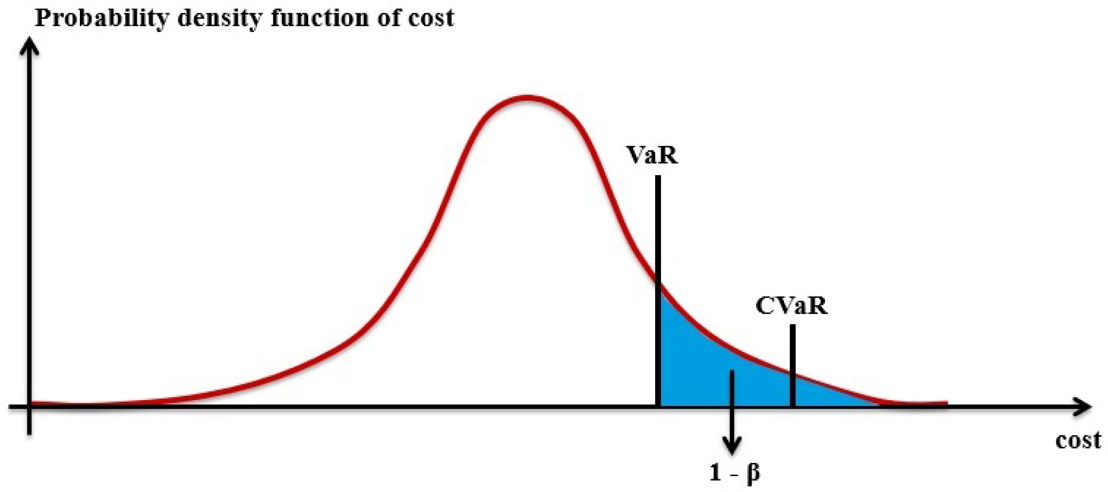
Figure 2.
Scenarios for the market electricity price.
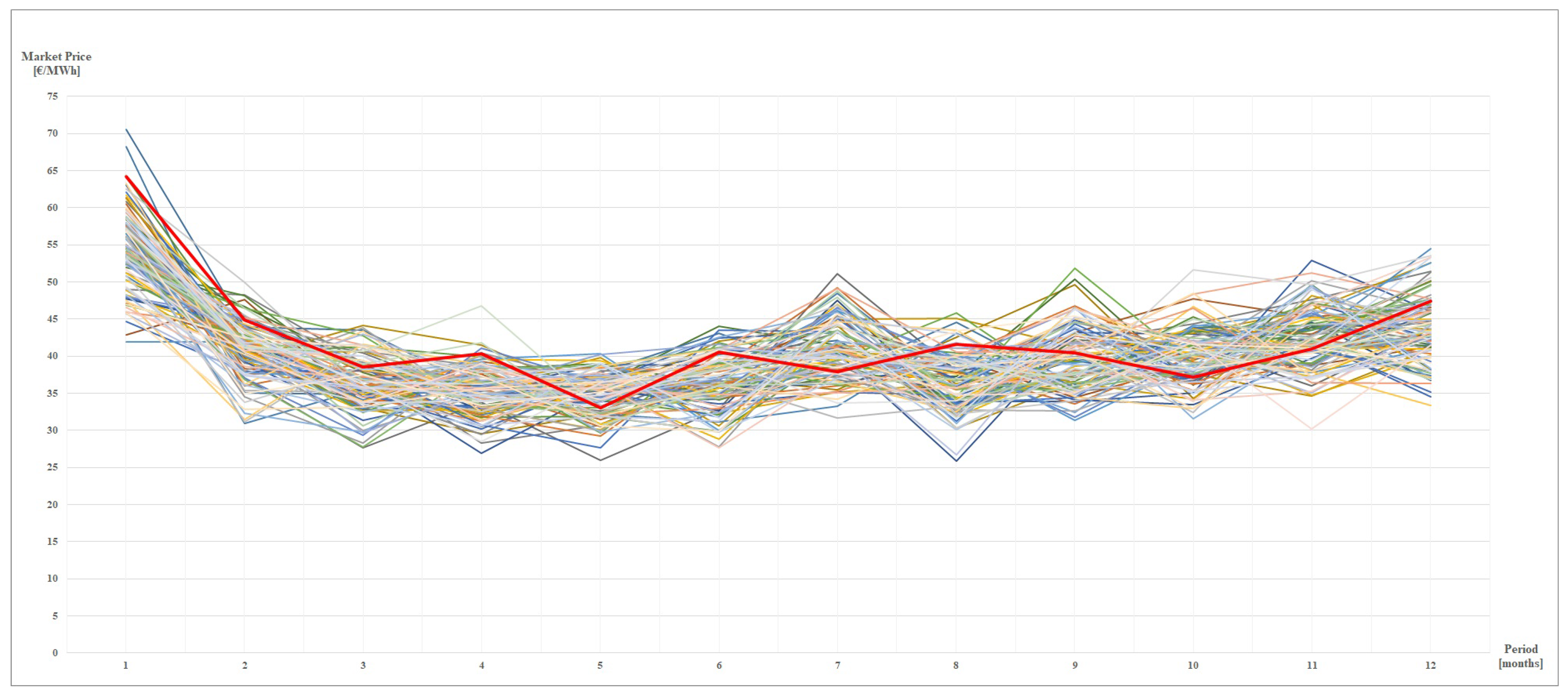
Figure 3.
Scenarios for the overall energy demand.

Figure 4.
Optimal procurement plan.

Figure 5.
Cost distribution.

Figure 6.
Trade-off between expected cost and CVaR.
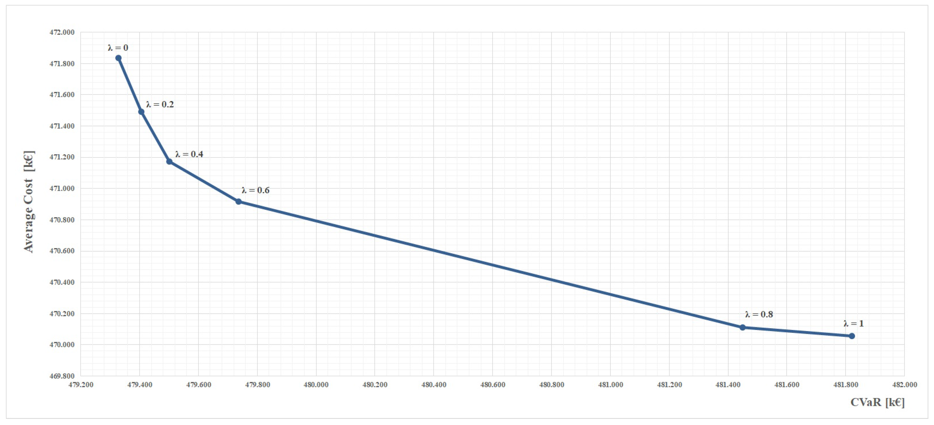
Figure 7.
Procurement costs.

Table 1.
Available bilateral contracts.
| Bilateral Contracts | 1 | 2 | 3 | 4 | 5 | 6 | 7 | 8 | 9 | 10 | |
|---|---|---|---|---|---|---|---|---|---|---|---|
| Average unit price (€/MWh) | F1 | 42.3 | 42.3 | 42.3 | 41.6 | 41.4 | 42.0 | 40.9 | 40.8 | 40.9 | 40.8 |
| F2 | 43.3 | 43.3 | 43.3 | 43.7 | 42.4 | 41.3 | 41.3 | 40.9 | 40.9 | 41.4 | |
| F3 | 35.8 | 35.7 | 35.6 | 35.6 | 35.1 | 34.6 | 34.5 | 34.5 | 34.4 | 34.7 | |
| Fixed cost (€) | 650 | 675 | 575 | 375 | 725 | 650 | 625 | 500 | 550 | 850 |
Table 2.
Cost increase as function .
| Expected Cost (k€) | (k€) | |
|---|---|---|
| 0.85 | 457.48 | 465.89 |
| 0.90 | 462.83 | 471.42 |
| 0.95 | 470.84 | 479.61 |
| 0.99 | 481.03 | 490.20 |
| 1 | 485.45 | 494.58 |
Table 3.
Out-of-sample analysis ().
| Bil. Contract Cost (k€) | Market Cost (k€) | Production Cost (k€) | Total Cost (k€) | |
|---|---|---|---|---|
| 0 | 322.16 | −2.27 | 18.70 | 338.55 |
| 0.5 | 314.88 | 5.87 | 16.64 | 337.39 |
| 1 | 287.79 | 35.76 | 14.58 | 338.13 |
Table 4.
Cost comparison ([k€]) between decision approaches in out-of-sample tests ().
| 2S Model | CC Approach | |
|---|---|---|
| 0 | 365.64 | 338.55 |
| 0.5 | 364.69 | 337.39 |
| 1 | 364.99 | 338.13 |
© 2017 by the authors. Licensee MDPI, Basel, Switzerland. This article is an open access article distributed under the terms and conditions of the Creative Commons Attribution (CC BY) license (http://creativecommons.org/licenses/by/4.0/).
Share and Cite
MDPI and ACS Style
Beraldi, P.; Violi, A.; Bruni, M.E.; Carrozzino, G. A Probabilistically Constrained Approach for the Energy Procurement Problem. Energies 2017, 10, 2179. https://doi.org/10.3390/en10122179
AMA Style
Beraldi P, Violi A, Bruni ME, Carrozzino G. A Probabilistically Constrained Approach for the Energy Procurement Problem. Energies. 2017; 10(12):2179. https://doi.org/10.3390/en10122179
Chicago/Turabian StyleBeraldi, Patrizia, Antonio Violi, Maria Elena Bruni, and Gianluca Carrozzino. 2017. "A Probabilistically Constrained Approach for the Energy Procurement Problem" Energies 10, no. 12: 2179. https://doi.org/10.3390/en10122179
Note that from the first issue of 2016, this journal uses article numbers instead of page numbers. See further details here.