Hydro Power Reservoir Aggregation via Genetic Algorithms


Department of Electric Power Engineering, NTNU, 7491 Trondheim, Norway
*
Author to whom correspondence should be addressed.
Energies 2017, 10(12), 2165; https://doi.org/10.3390/en10122165
Submission received: 10 November 2017
/
Revised: 14 December 2017
/
Accepted: 15 December 2017
/
Published: 18 December 2017
(This article belongs to the Special Issue Hydropower 2017)
Abstract
:Electrical power systems with a high share of hydro power in their generation portfolio tend to display distinct behavior. Low generation cost and the possibility of peak shaving create a high amount of flexibility. However, stochastic influences such as precipitation and external market effects create uncertainty and thus establish a wide range of potential outcomes. Therefore, optimal generation scheduling is a key factor to successful operation of hydro power dominated systems. This paper aims to bridge the gap between scheduling on large-scale (e.g., national) and small scale (e.g., a single river basin) levels, by applying a multi-objective master/sub-problem framework supported by genetic algorithms. A real-life case study from southern Norway is used to assess the validity of the method and give a proof of concept. The introduced method can be applied to efficiently integrate complex stochastic sub-models into Virtual Power Plants and thus reduce the computational complexity of large-scale models whilst minimizing the loss of information.
1. Introduction
Producing electrical energy from hydro power shows two unique characteristics that no other alternative form of electricity generation offers. For one thing, the renewable, free inflow and the long plant lifespan allow for nearly expense-free production; for another thing, generation units can be interdependent due to physical interconnection of their waterways. Such serial correlation of hydro power reservoirs is the main focus point for efficient scheduling of hydro power dominated systems. The main target is to anticipate uncertain hydrological inflows and coordinate interconnected reservoirs to fulfill main targets such as optimal load generation scheduling under consideration of sub-targets such as spillage minimization and sustaining reservoir limits. Several approaches are proposed in literature, whereas stochastic problem formulations represent the bulk of current methodologies.
An early example of such a formulation is given in [1], which demonstrates how to approximate the expected cost and use a back- and forwards recursion to align those expectations over the time periods. Considering prices as external uncertain factors allows for them to have similar methods applied on [2]. This price taker decision results from a separation in bidding and scheduling models that are state of the art in hydro power dominated systems [3]. Literature offers a multitude of financial models to determine the economic side of this problem [4] and thus establish price scenarios that can be used as (stochastic) inputs to conduct scheduling of units in river basins [5]. In setups with several non-interconnected subsystems consisting of correlated hydro power systems, subsystems are traditionally aggregated and represented by single unit approximations. In other words, to increase computational efficiency (and thus reduce computation times [6]), whole river basins are aggregated to be represented as single units in a Virtual Power Plant setup. After the planning is conducted for this setup, the river basin is then calculated in detail [3] to determine specific schedules of the plants. Techniques to derive those aggregates are manifold: Ref. [7] derives a model intended for Stochastic Dual Programing, which uses discretization of inflows. Refs. [8,9] analyze the correlation between the reservoirs in a stream to derive an operating policy for an aggregated system. Refs. [10,11,12] extend on those approaches by deriving trajectories of the total system based on individual members to control several reservoirs simultaneously. Ref. [13] proposes an ‘equivalent formulation’ of a hydro power system, where step-wise bounds are applied on an interconnected system in order to both reduce size and minimize error. Ref. [6] builds on this formulation allowing for a preselected “skeleton” of a river system to have its values adjusted according to an original system of larger size. Similar to our approach, it uses Karush Kuhn Tucker conditions to solve the bidding-sub-problem and nests this optimization model in a larger, non-convex error-minimizing parameter fitting problem. By applying deterministic samples instead of incorporating uncertainty and market/price interactions, we are able to solve the sub-problem as a linear scheduling problem and, compared to [6], without complementarity conditions. This, in combination with a scenario generator, allows for a larger sample size, which in turn allows more in depth training of the applied learning algorithm. In addition, there is no necessity for a pre-selected “skeleton” as the algorithm in our methodology decides on the resulting shape of the equivalent system by itself.
This methodology as proposed in the following sections applies principles from the above mentioned aggregation techniques within a machine learning framework [14,15,16] that serves as a master problem with the objective to fit an aggregated system to a non-aggregated benchmark system. Several approaches have been proposed to use meta-heuristics to e.g., approach non-linear [17,18] or stochastic [19,20] hydro power scheduling problem formulations. Nevertheless, available literature offers no concept that applies similar methods for solving this parameter-fitting problem as the novel method presented below does. However, a characteristic of metaheuristics is the strong dependency on the choice of parameters [14,16], thus the results’ quality is limited by the quality of the applied tool. Nonetheless, the underlying framework provides a tool to incorporate in future applications building on more sophisticated machine learning techniques and methods. In addition, the model assumes that there is a sufficiently large amount of data to construct samples that accurately reflect the distributions of stochastic parameters. Especially for newer systems, this might not be the case and might limit the quality of the results.
2. Implications of Reservoir Capacities
Originally introduced in [21] and extended in [22], Hveding illustrates that the (water) value of hydrological inventory in hydro power dominated systems is a result of the physical limitations of storage—the reservoir capacities and . This physical limitation is of special importance for multi-reservoir systems where some reservoirs might reach their capacity limits faster than others and therefore cause a bottleneck in an interconnected system, indirectly capacitating the downstream generation units.
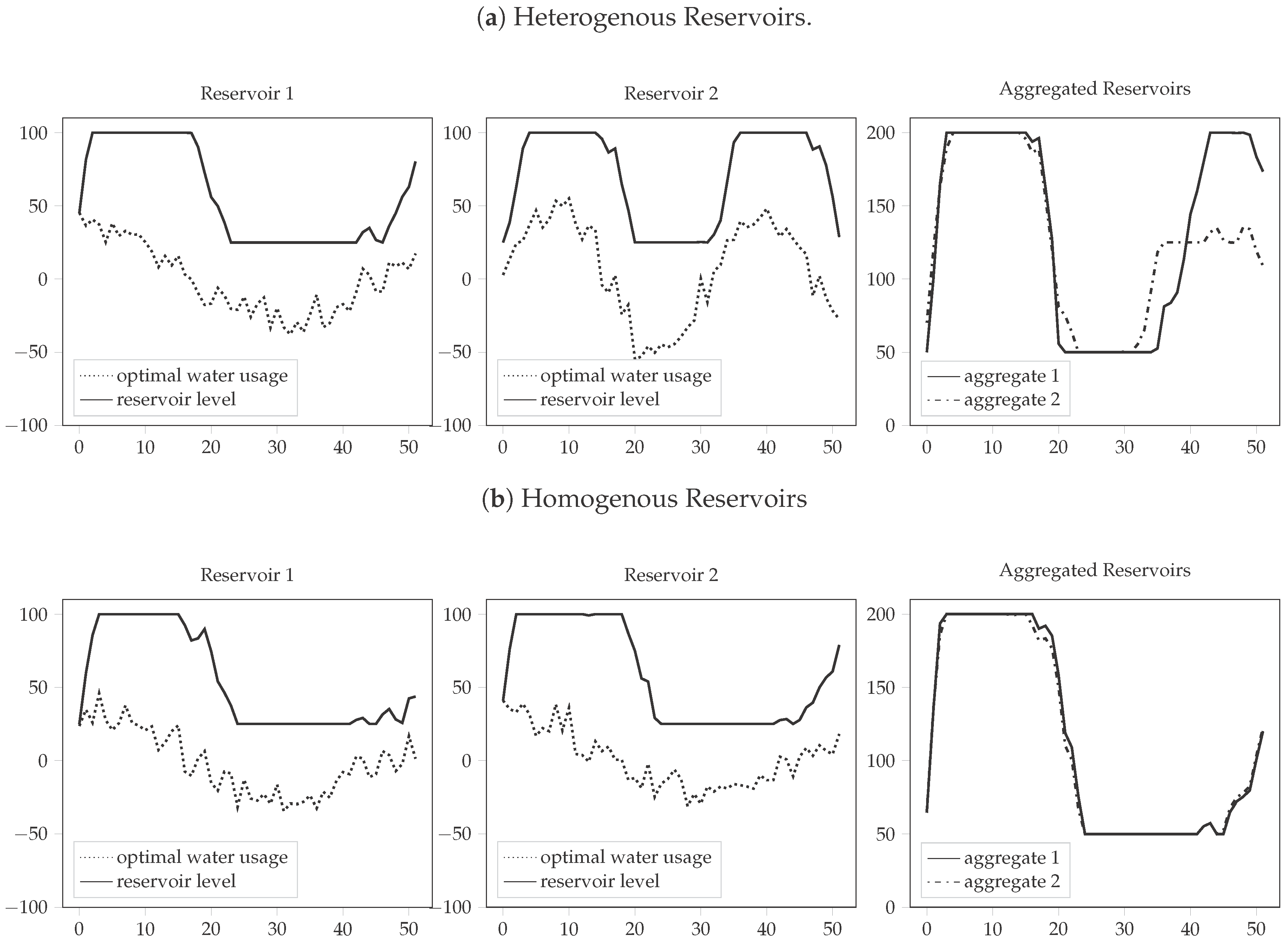
In addition to that, different reservoir behaviour can cause irregularities in aggregation. Figure 1a illustrates that in the example of two units with that gain and lose inventory over the course of 52 periods (this change is denoted as ). There is no correlation assumed between the reservoirs. Two methods are used to derive a single reservoir, which aims to imitate the behavior of both reservoirs:
Equation (1a) demonstrates the aggregated option, where both capacities and water usage are added to derive the new inventory, whereas Equation (1b) defines the “optimal” aggregate—summation after calculating individual reservoir levels. It is obvious that Equation (1b) does not fulfill the purpose of aggregation since it still requires individual computation of the levels of every single reservoir in the system. As Figure 1a shows, however, that the summation method presented in Equation (1a) can lead to incorrect behaviour in cases where some reservoirs are congested whereas others are not. This irregularity cannot be dealt with by adjusting the size of the reservoirs in the aggregation, it requires adjustment of the water usage curves (which is determined by inflows, generation capacities, etc.). The dependency on uncertain factors and other irregularities such as irrigation makes this adjustment itself a complex task.
Reservoirs with homogenous behavior, however, might show a small loss of information when being summed up and require little further adjustment to the other system parameters. Similar inflow patterns and usage trajectories might lead to joint operation resulting in similar outcomes than individual operation. Such a case is shown in Figure 1b. Moreover, some reservoirs might even behave different depending on applied scenarios. The following sections will aim to introduce a framework able to handle such irregularities.
3. Deterministic Hydropower Scheduling Equivalent
As mentioned above, scheduling of hydro power is subjected to various stochastic factors—all originated in both market circumstances and external causes. Below, it will be assumed that a river basin with a number of power stations is subject to uncertainty . Specifically, three uncertain parameters are considered in the medium-term formulation of the hydro power scheduling problem presented here: the market clearing price , the cost factor or water value (the formulation of water value used here deviates from traditional models. As the presented model is of deterministic nature, the water value was considered a penalty/incentive value of using/storing water in a certain period t. As mentioned later, this value can be kept at 0, but altering it seasonally increases the accuracy of the later presented master problem.) of using inventory and the hydrological inflow . This leads to an operation function in the form of:
presents the optimal operational strategy for all considered scenarios . It is now assumed that there exists a single scenario for , whereas , i.e., a finite time period. Such a scenario can be obtained from long-term scheduling approaches such as the method presented in [3]—explicitely stating price curves, water values and hydrological inflow. This results in the following formulation:
For the hydro power scheduling problem, four potential levers can be chosen as decision variables: the spilled hydrological inventory, the hydrological inventory used in generation, the stored hydrological inventory and the generated power. Deciding on definitive values for two of them suffices to derive the other two as functions of them. Traditionally, the chosen variables are of physical nature—spillage and release. The framework presented here deviates from that traditional view by using power in instead of hydrological inventory in as a decision variable. Due to the (stepwise) linear relationship in the generation steps, both approaches are valid and solely a matter of choice of the model user. Considering that the decision variables are denoted as generated power q and spillage s, where , then the extended form of the deterministic equivalent (in other words: the problem for a specified scenario ) of the hydropower scheduling problem can be formulated as:
This equivalent formulation can be solved for various samples . Even though Jensen’s inequality (i.e., for convex ) constitutes that there is (at least a potential) loss of information, the possibility of solving a larger sample size (required to train the later presented learning algorithm) was considered favorable to the computationally more demanding stochastic formulation. The objective function (4a) is concerned with the maximization of profit in the total system. Capacity constraints are imposed on generated power (4c), generation discharge steps (4d) and reservoir inventory (4h). Constraint (4e) ensures time consistency of the reservoir inventory under consideration of utilized inventory (4f) and received inflow (4g). It considers starting and ending inventories that lie outside of the analyzed time frame , thus . Using for and in (4e) ensures that hydrologic inventory requires a time period to transition from one power station to the next. The time steps t can be chosen in any fitting resolution ranging from hours to weeks. The latter applied medium-term case study uses weekly time steps. Higher resolution would certainly have a positive effect on result quality but also increase computation times. The physical network is modeled through a network matrix F, whereas symbolizes that 100% of the shed inventory in power station j reaches station i. Every generation units discharge is split into a number of discharge points , which are required to be stepwise linear [23]:
To ensure problem convexity, linear cost functions denoted by the water values W can be assumed:
The water values thus provide additional incentives to shed or save water in specific periods. For the deterministic model, it is possible to keep those at a steady level of ; adding different scenarios, however, can support the master problem proposed in the next chapter to find a more accurate portrayal of the original system.
A finite time horizon requires starting and ending inventory assumptions in (4e), which are met in the form of:
Spilled—i.e., shed but unused—hydropower capacity behaves as a slack variable in (4f). Considering that this “waste” of a natural resource should be minimized (which could e.g., represent a sub problem) and keeping the slack variable in the problem setup could create distortion in the dimensions of the amplified model represented in the next section, it was chosen to be bounded as:
Even though spillage is not beneficial for the system, it is still an important slack variable for scenarios with high inflows. Appendix A explains the reasoning behind this and the resulting need for a capacity constraint on this variable in detail.
4. Scaleable Deterministic Model
The aim of the presented framework is to reduce the number of power stations within the network whilst keeping the behaviour of the system intact. This is done through introduction of a binary cutting vector C:
As it can be observed, vector C scales the capacities of the power stations and reservoirs. In addition, rerouting of the river stream has to be conducted, transforming . In order to apply a metaheuristic to solve the parameter fitting problem, leverages for generation , inflow and reservoir size have to be introduced. This results in the following problem formulation:
Similar to [6], this presents a bilevel optimization problem with as the lower level decision variables and as the decision variables of the upper level problem. Even though the lower level problem is linear and thus convex, the upper level optimization problem (the later defined parameter fitting problem) is a non-convex multi-objective formulation, which requires appropriate techniques to yield an acceptable (local) optimum.
It can be noted that , , results in the unscaled model . This system can be used to provide a benchmark, as it represents the “natural state” of the problem. Deviating from this original state creates a different system setup, whereas the C vector denotes the cuts of reservoirs and generation units and and can be used to scale the leftover plants in order to compensate for the lack of capacity caused by the removals. Furthermore, follows the concept of fuzzy sets as presented in [24]—all original inflow scenarios are “mixed” to create new inflow curves in the remaining reservoirs that ensure that the seasonalities from the original scenarios are kept. In addition to the presented reformulation of the deterministic problem, the starting inventories for the finite time horizon presented in (7) have to be adjusted accordingly:
Next, a framework will be presented that aims to use the scalable form in order to increase system compactness.
5. Parameter Fitting
The purpose of the parameter fitting is to reduce the number of power stations, i.e., decrease , whilst keeping the general “behavior” of the system similar to the initial state . It is assumed that similar outcomes in every single scenario for both scaled and unscaled problems lead to similar outcomes for the optimal solution, i.e.,
A number can be assigned that limits the maximum number for stations that can be in the aggregated system (the algorithm is free to choose less, however). Thus, the problem can be reformulated to:
However, fitting the system parameters by minimizing the deviation in objective value might not accurately represent the strategy of the system as might vastly differ in the Left Hand Side (LHS) and Right Hand Side (RHS) problem in Equation (12) and thus render the result useless for its intended purpose.However, by introducing weighting factors—which are usually considered predefined system parameters— it is possible to define a feedback function in the form of:
Variables marked with ∗ denote the optimal solution of , whereas refers to , respectively. The quadratic term stems from using the squared error in order to ensure stronger impact of larger deviations. As mentioned above, the four levers describing the system are: the spilled hydrological inventory, the hydrological inventory used in generation, the stored hydrological inventory and the generated power. As the scaled model keeps the linear relation between used inventory and generated power intact, only one of those two—the generated power—was added to the master problem. The reservoir inventory—even though not a decision variable in the sub-problem—still has to be added as a performance indicator in the master problem, as its extent can be solely influenced by reservoir sizes without altering other components in the system. It can be observed that Equation (14) approximates a multi-objective problem (fitting both strategy and objective results) as a single-objective problem. This feedback function can be used to apply heuristics levering the scalable model. A genetic algorithm fulfilling this role will be presented in the following section.
6. Genetic Algorithm
It can be assumed that and are predefined inputs to the model. The techniques to derive them applied here are presented in Appendixes Appendix B and Appendix C, respectively.
The algorithm to solve the multi-objective optimization problem shown in Equation (14) as an upper level problem, with the deterministic optimization model as a lower level problem, is presented in Figure 2. The chosen meta-heuristic to approach the problem was that of a genetic algorithm [14,15,16]. Such methods, however, tend to produce skewed results when confronted with capacity constraints. Even though they are able to handle inequality constraints, reformulating strict bounds as penalty values leads to a smoother performance: an algorithm with capacity constraint reaching the bound can only move below/upwards (depending if the bound is a maximum/minimum), whereas a penalty function can choose to move away from the bound or “solidify” the bound. Thus, Equation (14) was reformulated to establish the feedback function:
The new weight factor has to be chosen sufficiently high to outrank the remaining weights by a multitude. As it is the only weight that is connected to the problems’ feasibility, the constraint was specifically chosen to outrank the remaining weights, whose associated constraints solely have an impact on the optimality region and cannot render the problem infeasible. As the feedback function gives quantified information about how close one particular solution is to the benchmark solution of the original system, it can be used to rank the solution in terms of fitness. Thus, it can also be referred to as fitness function. A genetic algorithm defines a number of agents p in a population P that all individually try to minimize this fitness function. Those agents learn both from each other and their past actions via three tools:
- mutation: changes in decision variables based on random variables drawn from predetermined possibility distributions,
- crossover (”mating”): merger of decision variables of “parents” to establish new “children” that are added to the population,
- selection: removal of members of P by comparing their fitness values.
The applied algorithm is an extended version of the tool presented in [25] and will be introduced in the following sections.
6.1. Individual
A population P consists of several individuals p, each being characterized by their constellation of decision variables. The extended form of the decision variables shows their dimensions: (dimension: I), (dimension: I), (dimension: I), (dimension: ). Thus, a single individual p has the size of . This shows that the size of the upper level decision problem is mostly dependent on the amount of power stations incorporated. It has to be pointed out that the amount of discharge steps does not scale with the complexity of the problem, as long as the condition of stepwise linearity in Equation (5) is fulfilled. Initialization of each individual was chosen to be the unscaled model presented in Section 4: .
6.2. Feedback Function
As mentioned above, the multi-objective feedback function aims to provide a basis to rate and wage the outcomes of similar scenarios in systems with different parameters. Appendix A illustrates how, due to restrictions on slack variables, some scenarios with inflows that are too high can result in infeasible problems . Those have to be sorted out of the scenario sample set . However, by under-dimensioning the decision variables of the upper level problem (15), lower level objective function can become infeasible for a scenario . Thus, this requires a reformulation of the upper level objective function with addition of a new weight factor :
6.3. Algorithm Parameters
The parameters of the algorithm are strongly based on the problem setup and require adjustment and fitting. For the case study presented in the next section, the following setup was used:
Crossover [15] was conducted by using the principle of two-point crossover: two randomly selected points in the sequences (the “chromosome”) of the individuals are chosen, where they are cut and merged into two new individuals that are added to P.
Adjusting of the crossed individuals was conducted through mutation [16]. The continuous variables v were alternated based on a Gaussian distribution with a mean of 0 and a variance of , where denotes the current generation of the population P. The probability of mutation was selected as for each tupel of every individual. Having the variance depend on the current generation follows the concept of simulated annealing [14]. The binary variables C were alternated with a probability of .
The chosen selection was tournament selection as proposed in [16] with a tournament size of a tenth of the starting population. Two forms of population reduction were used:
- -
- Due to crossover, the increase is exponential (with every generation, the size of the population increases by 100%) and the model requires large quantities of scaling; the population was collapsed to 67% of its size after each generation (via tournament selection as denoted above).
- -
- To eventually collapse the population to a single individual, a second set is required. On those scenarios , no mutations and crossovers are applied. The rate of collapse per generation can be calculated as .
7. Case Study
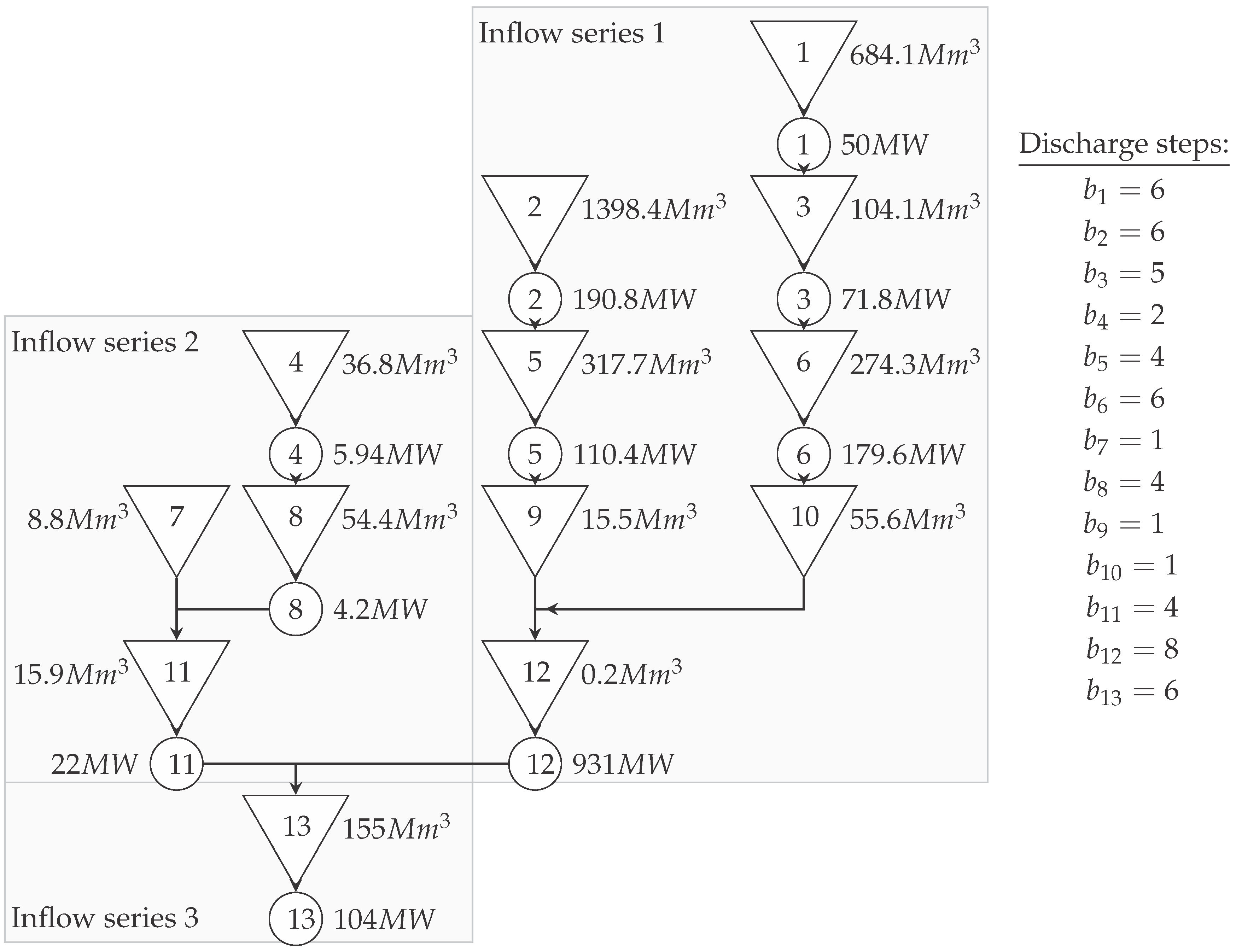
The selected river basin for the case study was the "Sira-Kvina" system in southern Norway presented in Figure 3.
The system consists of 13 units with different constellations ranging from seasonal reservoirs to run-on-river plants. Due to the dependency on accurate weight selection, the algorithm loses accuracy if is chosen to be too low. Thus, depending on the cases, preliminary adjustment to the system and thus preliminary cuts can be conducted. One characteristic to support decisions on such cuts is the degree of regulation () as presented in [23]:
Low would result in reservoirs that have to continuously shed inventory in order to not overflow, where a high would describe a reservoir that is able to hold inventory over longer time frames in order to catch price spikes. The former act simply as bottlenecks in the river streams and can be cut without changing the behavior of the system drastically, whilst the latter have to be kept to keep the system characteristics. This “manual” selection of cuts follows a more traditional, rule-based approach as applied in the papers presented in the introduction. The (manually chosen) reservoirs for preliminary cuts were the reservoirs #1, #2, #12 in Figure 3 with respective of 0.81, 0.34, 0.05, respectively. Thus, the respective cutting variables had to be fixed, i.e., .
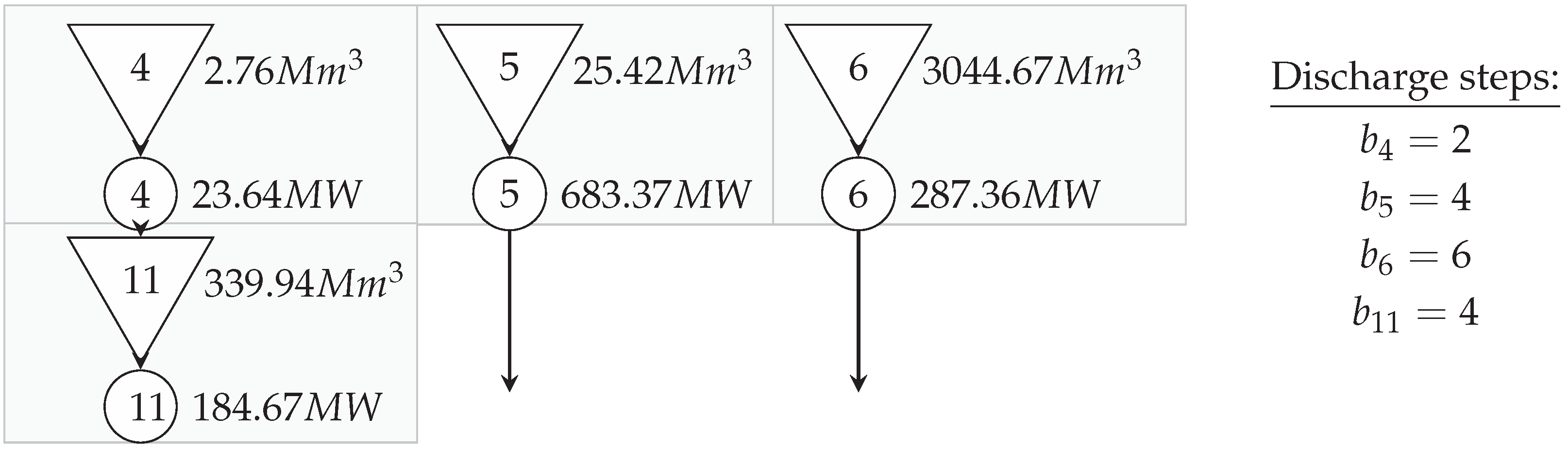
Figure 4 shows the resulting system after being reduced to a third of the original number of plants. The algorithm parameters were a maximum population of 100 individuals with 55 starting individuals, 100 generations and weights of . Those weighting factors are chosen parameters and have to be predetermined by the operator applying the technique. Even though there exist techniques to systematically determine those weights, the weights in this case study were selected manually. Systematic determination of those factors would help to improve the end results yielded by the framework but were considered to lie out of the scope of this paper. The original reservoir size of a total of grew into , whereas the production capacity decreased from to . Removal of reservoir and station #13 resulted in a system consisting of three parallel independent streams, which shows a different approach to traditional pooling of an upstream into a downstream reservoir as presented e.g., in [26]. The computation times were below seven hours for an Intel i7-5600 CPU.
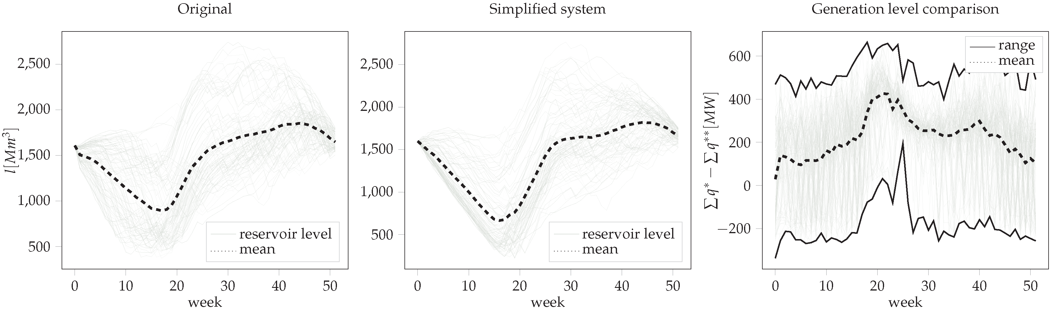
The results of the case study simulation are presented in Figure 5; light gray lines represent single samples , showing the reservoir levels for both the original and the aggregated system as well as a comparison of generation levels (with the minimum and maximum differences shown as boundaries). The results indicate that the similarities in behavior of both systems come closer in high inflow (“filling”) periods and diverge slightly stronger in low inflow (“emptying”) periods. A reason for that might be found in the degree of regulation decreasing for higher inflow and thus allowing a smaller range of dispatch decisions. However, the displayed results can be considered highly desirable, decreasing the complexity of a system with 54 discharge steps to a compact size of 16.
The results also indicate that using fuzzy sets to combine inflows into new inflow curves suffices to compensate for the irregularities mentioned in Section 2. However, as it can be seen within the first weeks of the simplified models’ reservoir decisions, they also show that releasing happens slightly faster and in steeper steps as in the original model. The reason for that is that bottlenecks—such as the reservoirs with low degree of regulation mentioned above—are removed from the system. One possible solution could be adding a time dimension to the scaling coefficient , transforming it into . Such a setup could adequately emulate system bottlenecks in certain periods t, leaving the problem non-congested for other periods. As implementation of such time-variant generation capacities is not considered in many industry-applications and is therefore difficult to implement [23], further research on the topic is recommended.
8. Conclusions
This paper presented a framework aimed to increase computational compactness of large scale hydro power systems. A deterministic linear approximation of the stochastic hydro power scheduling problem was used as a nested sub-problem within a multi-objective problem setup aiming on keeping behavioral consistency in a system with reduced size. Additional tools like a scenario generator and case analysis (selecting reservoirs on the basis of other parameters such as the introduced degree of regulation) were introduced as well, helping to refine the outcomes presented in the case study. The method presents a novel application of parameter fitting through evolutionary algorithms, which, in hydro power scheduling, were traditionally only used to analyze and filter input. In contrast, the proposed framework aims to alter the system itself in order to increase system compactness. Potential starting points for future work on the methodology are manifold as the master- and sub-problem are only connected through a single feedback function, giving the possibility for individually improving parts of the model whilst keeping the validity of the entire framework intact.
Acknowledgments
The research is a part of the Norwegian R&D project “Methods for Aggregation and Disaggregation” financed by the Norwegian Research Council (project no. 245269) and industry partners.
Author Contributions
Löschenbrand and Korpås designed the model and the case study; Löschenbrand analyzed the data; Löschenbrand wrote the paper.
Conflicts of Interest
The authors declare no conflict of interest.
Nomenclature
| Indexes: | |
| scenario | |
| generation unit/reservoir | |
| discharge steps of generation unit i | |
| t | time period |
| alternative time period | |
| Variables: | |
| generation | |
| spillage | |
| station cut | |
| generation leverage variable | |
| inventory leverage variable | |
| inflow leverage variable | |
| Parameters: | |
| market price | |
| maximum generation capacity of generator i | |
| maximum generation capacity of discarche step b | |
| hydrological inflow | |
| conversion rate | |
| maximum reservoir capacity | |
| water value | |
| water course matrix | |
| start period hydrological inventory | |
| end period hydrological inventory | |
| maximum spillage | |
| w | weight factor |
| maximum number of power stations/reservoirs in the system | |
| Functions: | |
| defines a function | |
| operation function of a system | |
| reservoir level | |
| profit function | |
| generation cost function | |
| periodic inflow | |
| periodic loss | |
| water course matrix with cuts C applied | |
| optimal operation | |
| Sets: | |
| scenario set | |
| P | population |
| Tuples: | |
| p | individual |
Appendix A. Maximum Spillage Constraint
In short form, the optimization problem in a single time stage can be presented as:
Here, the physical shedding of stored hydrological inventory denoted as s presents a slack variable, that relieves the reservoir size constraint. In order words, s will be used to compensate for non-sufficient production capacities to ensure that high inflow does not cause a breach of the maximum reservoir capacity . Spillage is not part of the profit function, thus a producer would prefer to use the stored inventory on production q instead, as it has a positive impact on the end result. As a result, producers would spill the exact minimum to just ensure avoiding breach of the reservoir capacities. In the scaled model presented in this paper however, the upper level problem comes in the form of the fitness function presented in (15) , defining pattern similarities in lower level decision variables of (10) as an objective. As a result, a heuristic could decide to compensate oversized capacity parameters by overusing slack variables. Such a result should be avoided by well defined weight parameters. Nonetheless, as such a scenario cannot be completely prevented, a bound on the slack variable s was chosen to be implemented. However, this situation can potentially lead to infeasible situations, in case of high inflow scenarios , that have to be sorted out of the sample set .
Appendix B. Scenario Generation
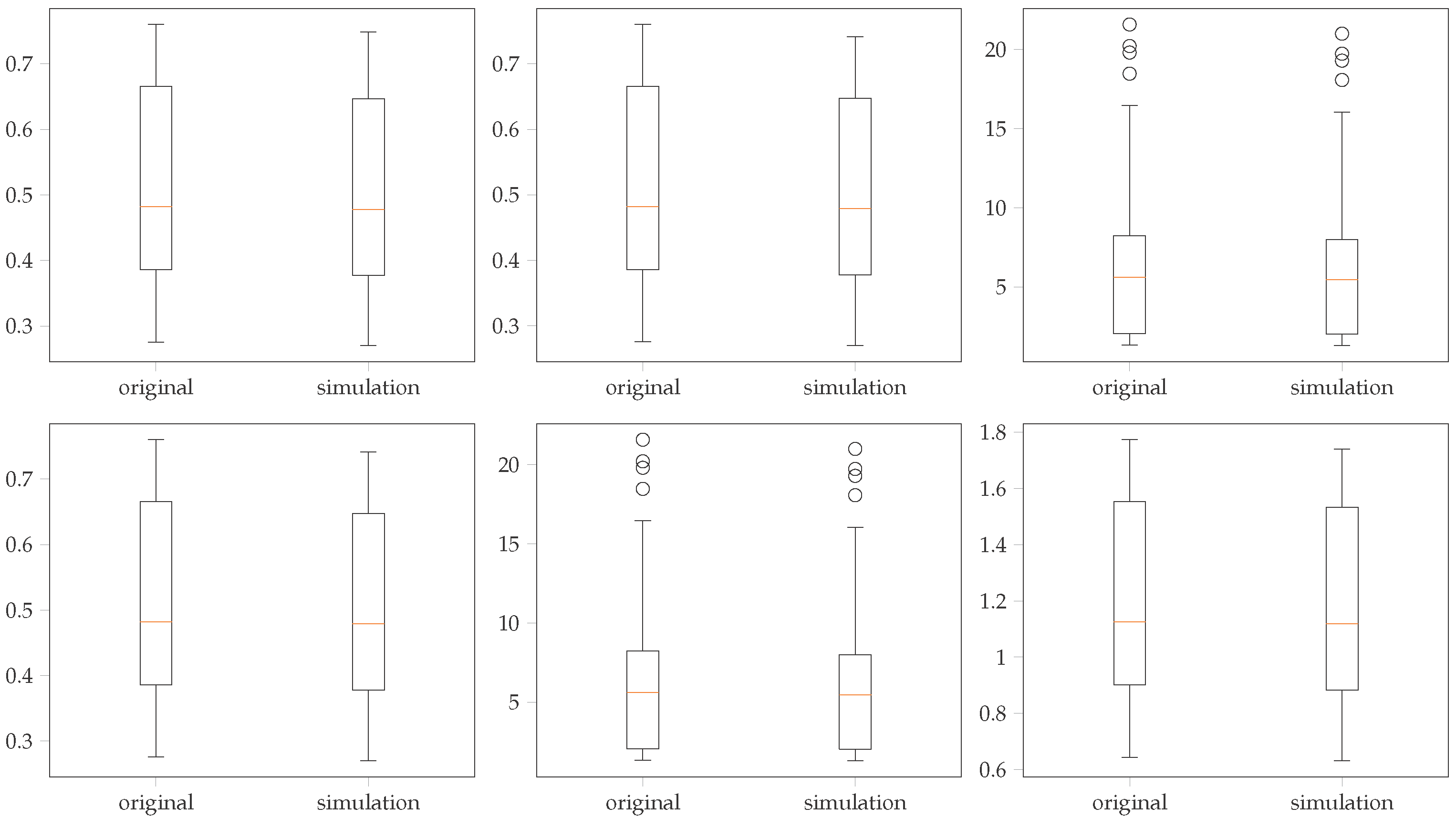
Denoting the amount of (time series) scenarios in a scenario set as , for an existing set of scenarios (i.e., obtained historical values), a representative set with has to be created (the reason for this higher cardinality is that a learning algorithm requires higher amounts of data that historical values are not able to offer in this quantity) that displays the distribution of accurately. A multitude of techniques have been proposed in literature [27,28]. In this paper, importance sampling, as presented in [29], in combination with a random walk (see [28]) was applied and will be debated below. As an example, consider a set of input parameters for a finite time period t, denoted as :
By using the average values and the standard deviations over all scenarios periods (A2a) and (A2b) establish a random walk, based on the random variables defined in (A2d) and (A2e). The parameters are predefined weights— defining the “step direction” of the random walk and the weight distribution between the selected benchmark scenario and the random walk. For the applied distributions, values of and proved to show the most satisfying results.
Figure A1.
Generated test scenarios.

To evaluate these factors, Figure A1 shows a comparison for six different inflow curves, each with 50 original input scenarios and 10,000 simulated sample scenarios.
Appendix C. Network Matrix Rerouting
Assume that reservoirs are numbered beginning at the top of the river basin and the physical limitations of water are only able to run downstream results in a notation of , effectively transforming F into a triangular matrix in the form of:
As mentioned before, the blocked reservoirs C constitute a decision vector. Thus, rerouting has to be conducted for the remaining, unblocked reservoirs. The algorithm to derive this rerouted water course from a given F and C can thus be formulated as:
In addition to the triangular form, this algorithm also requires . It can cope with reservoirs having both several destinations and source reservoirs.
References
- Pereira, M.; Pinto, L. Multi-stage stochastic optimization applied to energy planning. Math. Program. 1991, 52, 359–375. [Google Scholar] [CrossRef]
- Gjelsvik, A.; Belsnes, M.M.; Haugstad, A. An algorithm for stochastic medium-term hydrothermal scheduling under spot price uncertainty. In Proceedings of the 13th Power Systems Computation Conference (PSCC), Trondheim, Norway, 28 June–2 July 1999; pp. 1079–1085. [Google Scholar]
- Wolfgang, O.; Haugstad, A.; Mo, B.; Gjelsvik, A.; Wangensteen, I.; Doorman, G. Hydro reservoir handling in Norway before and after deregulation. Energy 2009, 34, 1642–1651. [Google Scholar] [CrossRef]
- Steeger, G.; Barroso, L.A.; Rebennack, S. Optimal Bidding Strategies for Hydro-Electric Producers: A Literature Survey. IEEE Trans. Power Syst. 2014, 29, 1758–1766. [Google Scholar] [CrossRef]
- Pereira-Cardenal, S.J.; Mo, B.; Gjelsvik, A.; Riegels, N.D.; Arnbjerg-Nielsen, K.; Bauer-Gottwein, P. Joint optimization of regional water-power systems. Adv. Water Resour. 2016, 92, 200–207. [Google Scholar] [CrossRef] [Green Version]
- Shayesteh, E.; Amelin, M.; Soder, L. Multi-Station equivalents for Short-term hydropower scheduling. IEEE Trans. Power Syst. 2016, 31, 4616–4625. [Google Scholar] [CrossRef]
- Valdes, B.J.B.; Filippo, J.M.D.; Strzepek, K.M.; Restrepo, P.J. Aggregation-Disaggregation Approach to Multireservoir Operation. J. Water Resour. Plan. Manag. 1992, 118, 423–444. [Google Scholar] [CrossRef]
- Archibald, T.; McKinnon, K.; Thomas, L. An aggregate stochastic dynamic programming model of multi-reservoir systems. Water Resour. Res. 1997, 33, 333–340. [Google Scholar] [CrossRef]
- Turgeon, A.; Charbonneau, R. An aggregation-disaggregation approach to long-term reservoir management. Water Resour. Res. 1998, 34, 3585–3594. [Google Scholar] [CrossRef]
- Turgeon, A. Solving reservoir management problems with serially correlated inflows. River Basin Manag. III 2005, 83, 247–255. [Google Scholar]
- Turgeon, A. Optimal rule curves for interconnected reservoirs. River Basin Manag. IV 2007, I, 87–96. [Google Scholar]
- Liu, P.; Guo, S.; Xu, X.; Chen, J. Derivation of Aggregation-Based Joint Operating Rule Curves for Cascade Hydropower Reservoirs. Water Resour. Manag. 2011, 25, 3177–3200. [Google Scholar] [CrossRef]
- Söder, L.; Rendelius, J. Two-Station Equivalent of Hydro Power Systems. In Proceedings of the 15th Power Systems Computation Conference (PSCC), Liège, Belgium, 22–26 August 2005; pp. 22–26. [Google Scholar]
- Bishop, C.M. Pattern Recognition and Machine Learning; Springer: Berlin, Germany, 2006. [Google Scholar]
- Michalewicz, Z. Genetic Algorithms + Data Structures = Evolution Programs; Springer Science & Business Media: Berlin, Germany, 1995. [Google Scholar]
- Siarry, P. Evolutionary Algorithms. In Metaheuristics; Springer International: Cham, Switzerland, 2016; pp. 115–175. [Google Scholar]
- Cai, X.; McKinney, D.C.; Lasdon, L.S. Solving nonlinear water management models using a combined genetic algorithm and linear programming approach. Adv. Water Res. 2001, 24, 667–676. [Google Scholar] [CrossRef]
- Zhang, X.; Yu, X.; Qin, H. Optimal operation of multi-reservoir hydropower systems using enhanced comprehensive learning particle swarm optimization. J. Hydro-Environ. Res. 2016, 10, 50–63. [Google Scholar] [CrossRef]
- Saad, M.; Bigras, P.; Turgeon, A.; Duquette, R. Fuzzy learning decomposition for the scheduling of hydroelectric power systems. Water Resour. Res. 1996, 32, 179–186. [Google Scholar] [CrossRef]
- Lee, J.H.; Labadie, J.W. Stochastic optimization of multireservoir systems via reinforcement learning. Water Resour. Res. 2007, 43, 1–16. [Google Scholar] [CrossRef]
- Hveding, V. Digital simulation techniques in power system planning. Econ. Plan. 1968, 8, 118–139. [Google Scholar] [CrossRef]
- Førsund, F.R. Hveding’s Conjecture: On the Aggregation of a Hydroelectric Multiplant—Multireservoir System. In CREE Working Paper; Oslo Centre for Research on Environmentally friendly Energy: Oslo, Norway, 2014; pp. 1–30. [Google Scholar]
- Sintef Energy Research. EMPS—Multi Area Power Market Simulator. Available online: https://www.sintef.no/en/software/emps-multi-area-power-market-simulator/ (accessed on 10 December 2017).
- Zadeh, L. Fuzzy sets. Inf. Control 1965, 8, 338–353. [Google Scholar] [CrossRef]
- Fortin, F.A.; De Rainville, F.M.; Gardner, M.A.; Parizeau, M.; Gagné, C. DEAP: Evolutionary Algorithms Made Easy. J. Mach. Learn. Res. 2012, 13, 2171–2175. [Google Scholar]
- Turgeon, A. A decomposition method for the long–term scheduling of reservoirs in series. Water Resour. Res. 1981, 17, 1565–1570. [Google Scholar] [CrossRef]
- Löhndorf, N. An empirical analysis of scenario generation methods for stochastic optimization. Eur. J. Oper. Res. 2016, 255, 121–132. [Google Scholar] [CrossRef]
- Glassermann, P. Monte Carlo Methods in Financial Engineering; Springer Science & Business Media: Berlin, Germany, 2003. [Google Scholar]
- Birge, J.R.; Louveaux, F. Introduction to Stochastic Programming, 2nd ed.; Springer: Berlin, Germany, 2011; pp. 135–149, 289–338. [Google Scholar]
Figure 1.
Aggregates for different Reservoir Types.

Figure 2.
Genetic algorithm flowchart.
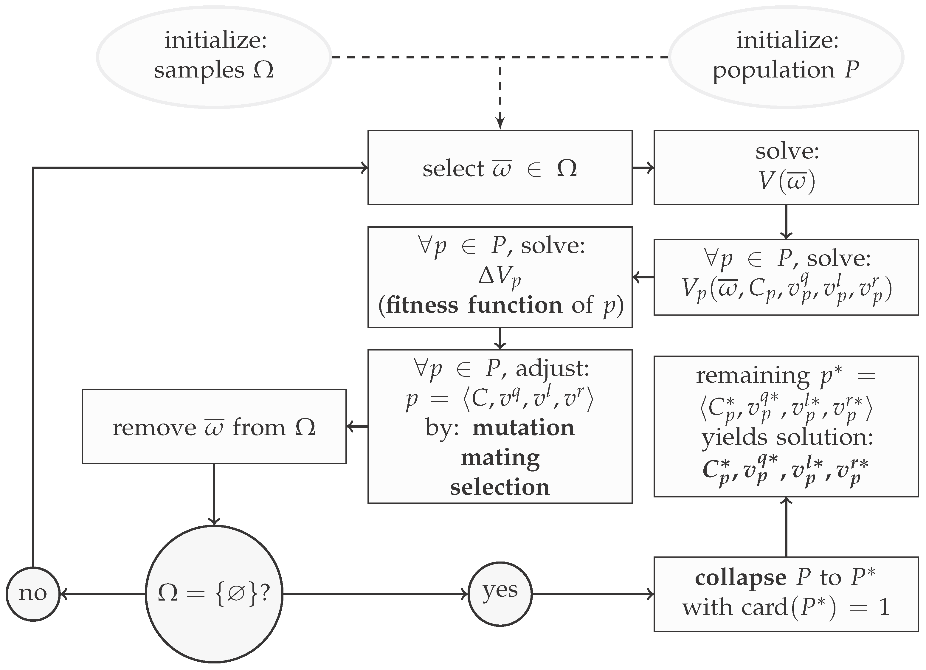
Figure 3.
Sira Kvina river basin.

Figure 4.
Simplified version of the Sira Kvina river basin.

Figure 5.
Result comparison of the original and simplified systems.

© 2017 by the authors. Licensee MDPI, Basel, Switzerland. This article is an open access article distributed under the terms and conditions of the Creative Commons Attribution (CC BY) license (http://creativecommons.org/licenses/by/4.0/).
Share and Cite
MDPI and ACS Style
Löschenbrand, M.; Korpås, M. Hydro Power Reservoir Aggregation via Genetic Algorithms. Energies 2017, 10, 2165. https://doi.org/10.3390/en10122165
AMA Style
Löschenbrand M, Korpås M. Hydro Power Reservoir Aggregation via Genetic Algorithms. Energies. 2017; 10(12):2165. https://doi.org/10.3390/en10122165
Chicago/Turabian StyleLöschenbrand, Markus, and Magnus Korpås. 2017. "Hydro Power Reservoir Aggregation via Genetic Algorithms" Energies 10, no. 12: 2165. https://doi.org/10.3390/en10122165
Note that from the first issue of 2016, this journal uses article numbers instead of page numbers. See further details here.